Radar isochrones as constraints on paleo–ice-sheet model simulations in two off-divide regions of East Antarctica

Radio-echo sounding of polar ice masses has revealed extensive isochrones that have primarily been used to constrain paleo-accumulation rates, geothermal heat flux, and changes in ice-sheet dynamics in stable regions of the ice sheet. However, isochrones remain under-utilised for calibrating ice-sheet models over large spatial scales, particularly in areas far from the stable ice divide where isochrones are typically more disrupted and models likely perform less accurately. Here, we illustrate the utility of isochrones for constraining paleo-ice-sheet simulations in two off-divide areas of the East Antarctic Ice Sheet; the Wilkes Subglacial Basin (WSB) and the Dronning Maud Land (DML) regions. Using airborne radio-echo sounding data from both legacy and newly acquired surveys, and the three-dimensional, thermo-mechanically coupled Parallel Ice-Sheet Model (PISM), we show that traced and dated isochrones are essential for calibrating model simulations in faster-flowing regions of the ice sheet. Associated with this paper are two datasets of nine and seven newly traced isochrones spanning the Holocene and Last Interglacial (∼ 4.8–128.4 ka) across the WSB and DML sectors, respectively, which may be used in future modelling studies to assess the paleo-evolution of the East Antarctic Ice Sheet. Using a commonly traced isochrone dated at ∼ 91 ka across both sectors, we simulate its modelled equivalent along two off-divide transects and discuss its utility for constraining the model. We highlight the influence of paleo-climate forcing and model parameterisation, which can lead to widely different model representations of isochrones despite producing reasonable present-day ice-sheet geometries that are consistent with observations. This study demonstrates that achieving a good present-day match in ice-sheet geometries in off-divide areas does not necessarily translate to an appropriate transient ice-sheet evolution in the model and thus emphasises the need to incorporate isochrones as boundary conditions in paleo-ice-sheet model simulations.

1 Introduction

In recent years, isochrones (also known as Internal Reflection Horizons, or IRHs) have been increasingly traced and dated across large swaths of the Antarctic Ice Sheet (AIS), mainly in association with the SCAR (Scientific Committee on Antarctic Research) AntArchitecture Action group (Bingham et al., 2025), which aims to build the first three-dimensional age–depth model of the AIS from isochrones. To date, these traced and dated IRHs have primarily been used to constrain paleo-accumulation rates (e.g., Leysinger Vieli et al., 2004; Eisen et al., 2005; Siegert et al., 2004; Neumann et al., 2008; MacGregor et al., 2009; Leysinger Vieli et al., 2011; Steinhage et al., 2013; Karlsson et al., 2014; Koutnik et al., 2016; Cavitte et al., 2018; Bodart et al., 2023) and ice-dynamical processes (e.g., Nereson et al., 1998; Catania et al., 2006; Leysinger Vieli et al., 2007; Catania et al., 2010; Leysinger Vieli et al., 2018; Chung et al., 2023).

Being often traceable across distances of several hundred kilometres, IRHs represent time-transgressive states of the ice sheet at large spatial scales. This sets them apart from other paleo-records such as offshore sediment cores (e.g., Hillenbrand et al., 2012; Larter et al., 2014), grounding zone wedges (e.g., Bart et al., 2017), radiocarbon-dated erratics on nunataks (e.g., Johnson et al., 2014; Nichols et al., 2019), and shells and bones on beaches (e.g., Braddock et al., 2022), or ice (e.g., Ruth et al., 2007; Buiron et al., 2011) and bedrock (e.g., Balco et al., 2023) cores. These proxies typically provide valuable local to regional snapshots of past ice-sheet dynamics (sediment cores) or extent (grounding zone wedges), elevation changes (radiocarbon dating of rocks and bedrock cores), or climate evolution at a single site (ice cores); however, their one-dimensional nature makes them susceptible to local biases (e.g., Johnson et al., 2021; Cavitte et al., 2023). Complementary to these proxies, isochrones uniquely provide both spatial and temporal calibration targets at the ice-sheet scale (Bingham et al., 2025), bridging a critical gap in available proxy information on past ice-sheet evolution.

Most modelling studies using traced and dated isochrones have focused on regions near ice divides and domes (e.g., Leysinger Vieli et al., 2004; Neumann et al., 2008; Koutnik et al., 2016; Cavitte et al., 2018; Beem et al., 2021; Bodart et al., 2023; Chung et al., 2023), primarily because of the stable ice-sheet conditions which lead to surface-conformable layering, and the nearby presence of ice cores used for dating these isochrones. However, such settings are also where models perform best, largely because ice dynamics at divide locations can be reproduced without the need for more complex physics (e.g., Waddington et al., 2007; MacGregor et al., 2009; Leysinger Vieli et al., 2011; Chung et al., 2023). Away from the interior, however, the vertical position of isochrones in the ice column will be the product of different internal processes influencing their elevations and geometries, including (1) ice-flow disturbances which can stretch or disrupt the planar geometry of IRHs, and (2) variations in surface and basal boundary conditions, such as surface accumulation, geothermal heat flux (GHF), or basal melting, which can alter the natural and slow compaction of isochrones over time; all of which require complex, multi-dimensional models to provide an accurate representation of their respective influences (Leysinger Vieli et al., 2007; Waddington et al., 2007; Leysinger Vieli et al., 2011; MacGregor et al., 2009; Sutter et al., 2021).

Continental-scale ice-sheet models employed for sea-level projections are usually not calibrated or constrained to match the paleo-evolution of ice streams and entire drainage sectors where ice-dynamical processes and boundary conditions are less well constrained (Born and Robinson, 2021; Sutter et al., 2021). However, this evaluation is critical for strengthening projections of future sea-level change, which are often subject to large uncertainties arising not only from climate scenarios but also to a large part from model initialisation and parametric uncertainties (Golledge et al., 2015; DeConto and Pollard, 2016; Seroussi et al., 2020; Siegert et al., 2020; DeConto et al., 2021; IPCC, 2023; Morlighem et al., 2024). Consequently, it is essential to assess these models' performance not only against present-day observations of ice-sheet geometry and flow, but also on their ability to reproduce past ice-sheet dynamics across a range of climatic states and transitions (Stokes et al., 2015; Kingslake et al., 2018; Bracegirdle et al., 2019; Johnson et al., 2021; Born and Robinson, 2021; Sutter et al., 2021; Lecavalier and Tarasov, 2025).

IRHs offer a powerful benchmark by allowing direct comparisons between observed isochrone elevations and geometries with those generated in large-scale paleo-ice-sheet simulations. Building on this potential, Born and Robinson (2021) and Sutter et al. (2021) presented the first direct applications of IRHs to constrain continental scale ice-sheet models for Greenland and Antarctica, respectively. These studies demonstrated that IRHs can complement more commonly used paleo-proxy reconstructions (e.g., Bracegirdle et al., 2019; Johnson et al., 2021; Lecavalier et al., 2023) to assess how well models reproduce past ice-sheet geometries.

This paper sits at the intersection of data-model integration by (i) providing two new datasets of traced and dated isochrones tailored to ice-sheet modelling purposes, and (ii) using a spatially extensive isochrone from these new datasets for comparison with its modelled equivalent. We begin by describing the airborne radar datasets onto which the isochrones were traced; summarise the process of tracing, dating, and assigning age–depth uncertainties; and then outline the ice-sheet model set-up. We then discuss our results, first describing the new database of isochrones traced on both legacy and newly acquired radar data across the Wilkes Subglacial Basin (WSB) and Dronning Maud Land (DML), respectively, and then turn our attention to a specific IRH traced and dated at ∼ 91 ka (before the present) and found across both WSB and DML regions, with the aim to assess how its elevation and geometry compares with its equivalent modelled isochrone. We conclude this manuscript with a series of lessons learned regarding modelling the paleo-history of the ice sheet in faster (and more dynamical) regions away from stable ice divides.

2 Data sets and methods

2.1 Airborne radar data

We used extensive radio-echo sounding data acquired over both the WSB and DML regions, as well as existing (i.e., published) IRH stratigraphies from the AntArchitecture database (Bingham et al., 2025) (data coverage of these existing stratigraphies is shown in Fig. 1) to trace and constrain the age of our isochrones. An important consideration when discussing the airborne radar surveys conducted over both WSB and DML is that whereas data over WSB were acquired mainly to obtain bedrock topography information in a grid-like fashion irrespective of ice-flow directions, the DML survey's main objective was to acquire data that is tailored to ice-sheet modelling applications. This means acquiring data along and across the main trunk of ice streams to (i) constrain mass flux and (ii) quantify the topographical imprint on isochronal stratigraphy which can be used more widely as a benchmark to assess simulated ice-flow patterns. Crucially, both sets of radar data intersect either prominent ice core locations or existing traced and dated isochrones previously extracted from coincident radar data (Winter et al., 2019; Cavitte et al., 2021; Franke et al., 2025b), thus enabling the accurate dating of our isochrones for future uses in ice-sheet models.

2.1.1 Legacy radar data over WSB

The primary dataset used over WSB is the 2005–2006 airborne radar survey “WISE-ISODYN”, acquired in a grid-like pattern (8 × 44 km spacing on average) by the British Antarctic Survey (BAS) using the 150 MHz Polarimetric Airborne Survey INstrument (PASIN) operating in two interleaved radar modes: a narrow-sounding, 0.1 µs pulse ideal for tracing isochrones in the upper 2 km of the ice at high resolution, and a deeper-sounding, 4 µs, 10 MHz chirp primarily used to pick the bed and trace deeper isochrones in the ice column (Frémand et al., 2022) (Table 1). This survey spans most of the WSB catchment with tie-points to the EPICA Dome C (EDC) and TALDICE (TALos Dome Ice CorE) ice cores, covering a total area of 730 000 km² and over 61 000 line-km (Fig. 1a) (Ferraccioli et al., 2009; Jordan et al., 2013; Frémand et al., 2022). For the purpose of linking our stratigraphy and increasing the amount of crossovers in crossover-poor areas of the survey, we also used opportunistic flight lines from: (i) CReSIS (Centre for Remote Sensing of Ice Sheets) NASA Operation IceBridge (OIB) MCoRDS (Multichannel Coherent Radar Depth Sounder) radar systems flown between 2013 and 2019 across the WSB to link major deep ice-cores in the region (MacGregor et al., 2021); (ii) Alfred Wegener Institute (AWI)'s EMR (Electromagnetic Reflection System) radar system flown between EDC and TALDICE ice-core sites in 2008–2009 (Winter et al., 2019; Franke et al., 2025a); and (iii) the University of Texas Institute for Geophysics (UTIG)'s HiCARS2 (High Capability Airborne Radar Sounder 2) radar system flown across WSB during the ICECAP (Investigating the Cryospheric Evolution of the Central Antarctic Plate) survey of 2011–2012 (Frederick et al., 2016; Young et al., 2016), all of which intersect the WISE-ISODYN survey grid in multiple places (Fig. 1a and Table 1). Importantly, existing IRH datasets were also previously extracted for the (ii) and (iii) surveys (i.e., Winter et al., 2019; Cavitte et al., 2021) which we make full use of here (see Sect. 2.2).

Table 1 Specifications of the airborne radar systems used in this study over the WSB and DML regions. For PASIN, we provide the transmit signal and range resolution for the pulse and chirp modes, respectively. All values for the range resolution are calculated using an electromagnetic wave speed in ice of 168.5 m s⁻¹. The horizontal sampling distances are typical values after post-processing. The vertical resolution of the chirp systems was calculated following CReSIS using a scaling factor k accounting for resolution degradation. TU HH in the table refers to the Hamburg University of Technology who designed the early EMR system for AWI.

In order to optimise and standardise the radar data, we removed the data between the air plane and the surface and flattened the ice surface using the previously traced surface pick. To facilitate our tracing, we also applied a gain function and horizontal averaging filter to reduce incoherent noise and enhance the brightness of isochronal stratigraphy, as previously done elsewhere on BAS PASIN data (e.g., Ashmore et al., 2020; Bodart et al., 2021). The vertical scaling of the radargrams were all adjusted to the BAS PASIN system range and sampling interval before being exported as SEG-Y files for isochrone picking.

Figure 1 Map of the airborne radar datasets used in this study for WSB (a) and DML (b). (a) BAS WISE-ISOYDN survey (white solid lines) and a combination of individual flight lines (grey dashed lines) from AWI (EMR 60 ns pulse data, otherwise referred to in this paper as “short-pulse”; 2008–2009), CReSIS (MCoRDS; 2013–2019), and UTIG (HiCARS; 2011–2012) (Table 1). (b) newly acquired AWI UWB (narrowband) CHARISO survey lines (white solid lines; 2023–2025) and a combination of individual flight lines (grey lines) from AWI's EMR (short-pulse; 1999–2003; solid lines) and AWI UWB (wideband mode; 2022–2023; dashed lines) radars (Table 1). Also shown are the previously published IRH datasets used in this study to tie our IRHs to existing age–depth profiles from Winter et al. (2019) and Cavitte et al. (2021) over WSB (a) and Franke et al. (2025b) over DML (b), with the colorscale representing the number of IRHs traced at a particular location (ranging from 1 to > 8 in both a and b). The background map shows modern ice-flow speeds from Rignot et al. (2017) in m a⁻¹. The black lines represent the RINGS/Bedmap3 grounding line from Pritchard et al. (2025) and the main drainage basin boundaries are from IMBIE (2018). The red triangles depict the location of the deep ice cores used in this study to date IRHs. The two yellow rectangles in (a) and (b) represent the location of profiles A-A' and B-B' shown in Fig. 4 for the data-model comparison. Abbreviations on (a) and (b) are as follows: EDC (EPICA Dome C), EDML (EPICA Dronning Maud Land), Mertz Glacier (MG), Ninnis Glacier (NG), Belgium's Princess Elizabeth Station (PE), Ross IS (Ross Ice Shelf), SRG (Sør-Rondanebreen Glacier). The blue star in (a) represents the centre of the main radar grid over WSB (coordinates: 71.65° S, 148.65° E), which is referred throughout the text as the ”WSB grid”. From this centre point, grid-west, grid-east, and grid-south are relative to the map grid orientation (i.e., right, left, down respectively from this blue star).

2.1.2 Newly acquired radar data over DML

Gridded (i.e., interpolated) bed-products such as Bedmachine or Bedmap (Morlighem et al., 2020; Pritchard et al., 2025) form the backbone of any ice sheet modelling efforts providing the necessary boundary conditions. However, acquiring radar data that is tailored to specific ice-sheet modelling needs (i.e., calibrating models with isochrones) is relatively rare in Antarctica, primarily because the main motivation of Antarctic radar surveying has historically been about mapping ice thickness and bedrock topography in an efficient manner. This has typically been characterised by surveying an entire catchment on a regular grid-like pattern, thus also facilitating optimized airborne geophysical data acquisition for gravimetry and magnetics (i.e., Fig. 1a). Because the geometry of deeper isochrones is heavily influenced by ice-dynamical processes such as ice flow in off-divide areas (Catania et al., 2005, 2006; Karlsson et al., 2009), models employed away from stable ice divides also need tailored information oriented perpendicular or parallel to the direction of flow to capture the imprint of fast ice flow often preserved in the geometry of isochrones. Additionally, ice-sheet models benefit from high-resolution bedrock data (ideally non-interpolated), which allow for direct evaluation along radar transects of how well the model reproduces observed features such as the surface, bed, and isochrones.

Where the WSB and DML regions differ is precisely in the motivation of acquisition; the WSB data were acquired to obtain ice-thickness and bedrock topography over large scales, rather than being explicitly guided by surface-flow directions, whereas the new DML lines were specifically flown to support modern ice-sheet modelling by capturing drainage pathways from the stable ice-sheet divide to the grounding line. Admittedly, modelling results over the WSB region are expected to show higher accuracy both spatially (across the catchment) but also directly along radar transects when compared to observations, because the WISE-ISODYN bed-elevation data (alongside many more detailed surveys in the area) are already included in the gridded product used to run the model. This means the model is better constrained because the boundary conditions are better known. However, because this information was not provided with a particular consideration to ice-streams direction, it is not straight forward to evaluate the model's ability to reproduce complex isochronal geometries directly along and across fast-flowing ice streams using existing radar transects. The WSB data largely compensate for this by providing a relatively dense radar grid covering a large area in contrast to the few individual flight lines acquired in the vicinity of the new DML lines (Fig. B1). Ideally, dense radar grids accompanied by individual along flow transects would perfectly address current modelling needs. Across DML where data coverage is generally poorer than over WSB (Fig. B1), we expect the surface, bed, and isochronal elevations to show a poorer match since the new DML lines were not included in the latest iteration of the Bedmap3 gridded product which is used to run the model. Nonetheless, this provides an opportunity to assess how well the model deals with drainage sectors in the absence of this underlying tailored radar data, a problem that is often overlooked when modelling at large scales in areas with poor data coverage.

In the austral summers of 2023–2024 and 2024–2025, the AWI UWB (UltraWideBand) radar system was flown on the Basler BT-67 aircraft Polar 6 (Alfred Wegener Institute, 2016) across prominent ice streams draining parts of the DML region as part of the CHARISO (Swiss (CH) Antarctic Research Initiative – ISOchrones in East Antarctic outflow regions) project (Fig. 1b and Table 1). The radar system was operated in narrowband mode (180–210 MHz range; 160 MHz sampling frequency; Table 1) and the data were processed using synthetic-aperture-radar focusing to enhance layering and reduce incoherent noise (for more details on the radar system and processing, see Rodriguez-Morales et al., 2013; Hale et al., 2016; Franke et al., 2025a). To facilitate tracing, we used the post-processed layer-enhancing AGC (Automatic Gain Control) version of the AWI radar data where possible and, as per WSB, we cut the data between the air plane and the surface and flattened the ice surface using the surface pick prior to exporting the data to SEG-Y file format. In addition to this, additional (non-CHARISO) radar data were also used to extend the layering in the upper sections of the DML lines near the ice divide, and across the main ice divide to link up specific isochrones with the EDML and Dome Fuji ice cores (Fig. 1b). These additional flight lines were acquired using the AWI UWB system operating in wideband mode (150-520 MHz range) in 2023–2024 (Franke et al., 2025b, a), and the older AWI EMR system (150 MHz) acquired between 1993 and 2003 and operating in short-pulse mode (Fig. 1b, Table 1) to connect the EDML and Dome Fuji ice cores (Nixdorf et al., 1999; Steinhage et al., 2013; Franke et al., 2025b, a).

2.2 Isochrone tracing, dating, and validation

2.2.1 IRH Tracing

We performed our isochrone tracing using the Schlumberger Petrel^® 3-D seismic software's in-built semi-automatic algorithm, which follows the local maxima in reflected power within a previously specified vertical window. The high density of crossovers between survey flight lines enabled consistent tracing of the same set of isochrones across extensive portions of the radar surveys (Fig. 1). This ensured that isochrones traced along the perpendicular grid direction matched their counterparts in the parallel direction, within the limits of system resolution and variations in isochrone appearance – such as brightness or clarity – across different radar systems (Winter et al., 2017; Bingham et al., 2025) (Table 1). Where necessary, we also made use of the 3-D capability of the software to find intersecting IRHs that were not visible in the 2-D view. Slightly different tracing strategies were employed for each of the WSB and DML regions.

For WSB, we first attempted to extend the existing isochronal stratigraphy datasets from Winter et al. (2019) and Cavitte et al. (2021) at key crossover points, starting at EDC and progressively travelling downstream along available radar lines into the main WSB grid (Fig. 1a). Due to disruptions in IRH geometries away from the dome region around EDC, and with our objective to trace as many IRHs away from the main ice divide, we also traced distinctively bright isochrones at the onset of the TALDICE ice core which were continuous over long enough distances and were not tied to known isochrones (Fig. 1a). The age of these new isochrones was transferred using the many crossovers in the radar data to expand the coverage grid-east into the main WSB catchment (Fig. 1a).

For DML, we mainly made use of the existing isochronal stratigraphy dataset from Franke et al. (2025b), which also included traced isochrones from other previous studies (Steinhage et al., 2013; Winter et al., 2019), to extend their stratigraphy onto the CHARISO lines and away from the main ice divide using available crossovers in the radar data (Fig. 1b). We found that most of the IRHs from Franke et al. (2025b) were also distinctively bright over the length of the CHARISO flight lines, except for the second shallowest and deepest isochrones we traced, which were both relatively bright but did not exactly correspond to the traced IRHs in the Franke et al. (2025b) dataset at our crossovers. We come back to this point in Sect. 2.2.3.

2.2.2 IRH depths and depth uncertainties

Once the isochrones were traced, we converted the value of each data point from the vertical range of the radar systems (t_IRH) to depths in metres below the surface (z_IRH), following

$$\begin{array}{}\text{(1)}& z_{\mathrm{IRH}}={\displaystyle \frac{t_{\mathrm{IRH}}{v}_{\mathrm{i}}}{\mathrm{2}}}+z_{\mathrm{f}},\end{array}$$

where v_i is the electromagnetic wave speed in ice in m s⁻¹ and z_f is the firn correction in metres calculated in Eq. (2) below.

Different values for v_i and z_f were used to convert to depths in metres, due to the different characteristics of both the radar surveys and the respective regions of East Antarctica in which these surveys and the accompanying ice-cores were situated. For WSB, we used a v_i value of 168.5 m s⁻¹ to match the depth of ice-thickness measurements obtained by BAS with the same value, and a spatially invariant z_f value of 14.6 ± 1.4 m as previously calculated by Cavitte et al. (2016) for EDC. For TALDICE, there are no reported z_f values, so we employed the firn correction equation from Dowdeswell and Evans (2004),

$$\begin{array}{}\text{(2)}& z_{\mathrm{f}}={\displaystyle \frac{K}{n_{\mathrm{i}}}}\underset{\mathrm{0}}{\overset{z_{\text{max}}}{\int }}\left({\mathit{\rho }}_{\mathrm{i}}-\mathit{\rho }\left(z\right)\right)\mathrm{d}z,\end{array}$$

where K is the coefficient calculated from Robin et al. (1969) (0.00085 m³ kg⁻¹) and later refined by Kovacs et al. (1995), n_i is the refractive index of ice (1.78), ρ_i is the density of pure ice (917 kg m⁻³), and ρ_z is the density at depth z using the TALDICE density profile for the upper 300 m of the core in kg m⁻³ (Buiron et al., 2011). Following Eq. (2), we found a z_f value of 9.5 m, which we applied to all IRHs dated at TALDICE. To this, we added an approximate 2 % uncertainty error in density values at TALDICE, as previously suggested by Barnes et al. (2002) and Cavitte et al. (2016) for EDC and Vostok ice cores, amounting to a z_f uncertainty value at TALDICE of ± 1.7 m.

For DML, we used a v_i value of 169.5 m s⁻¹ to match the depth in metres of the radar-derived products from AWI in the region (e.g., Franke et al., 2025b, a) and spatially invariant z_f values of 13 ± 2.5 and 15.5 ± 0.5 m for IRHs dated at EDML and Dome Fuji, respectively, as previously calculated by Wang et al. (2023) and Franke et al. (2025b) based on shallow firn cores and Eq. (2).

We followed the methods of Cavitte et al. (2016), Winter et al. (2019) and Bodart et al. (2021) to calculate the depth uncertainties associated with our isochrones. These uncertainties originate mainly from three components: (i) the range resolution of each radar system (provided in Table 1), (ii) the uncertainty associated with the speed of radar wave in ice, which can be approximated to 1 % based on dielectric permittivity measurements in dry ice (Bohleber et al., 2012); and (iii) the uncertainty associated with the firn density corrections used. Assuming these uncertainties are not correlated, the total IRH depth uncertainty is calculated as the root-sum-square error of these three uncertainties. Because the largest uncertainty in IRH depth will be on the deepest (and thus oldest) isochrone, we report here the maximum IRH depth uncertainty on the oldest isochrone in both sectors, which is 13.8 m for the oldest IRH traced on PASIN over WSB and 7.0 m for the oldest IRH traced on the AWI UWB over DML. Given that this represents a worst-case uncertainty across our datasets from the radar uncertainties alone, we also provide depth and age uncertainties for each IRH at the specific ice-core sites (see Sect. 2.2.3 and Table 2). These numbers represent a simple measure of the maximum IRH depth uncertainty that dataset users can expect from the radar depths alone. It is worth noting that these uncertainties are up to an order of magnitude smaller than what current generations of ice-sheet models can currently represent realistically when their own uncertainties are taken into account (i.e., see Sect. 3.2.2, Table C1, and Sutter et al., 2021). In the modelling domain we thus treat traced and dated isochrones such as those presented here as absolute ground truth for model calibration. We do not consider errors associated with our picking as this is difficult to estimate, nor do we account for snow accumulation or snow re-distribution between survey years. Considering previous estimates of picking uncertainties and travel-time-to-depth conversion from past studies, we expect these unquantified uncertainties to be smaller than the range resolution of the radar systems used here for the area and timespan considered. However, to ensure that IRHs are, on average, the same across intersecting transects, we conducted a crossover analysis of IRH depths across both WSB and DML radar lines (see Appendix A), which showed that median crossover errors are between 3 and 18 m over WSB (Fig. A1) and 1 to 8 m over DML (Fig. A2).

2.2.3 IRH ages and age uncertainties

Following the conversion to depth, we proceeded to date the isochrones closest to intersecting ice-core locations using the new AICC2023 ice-core chronology (Bouchet et al., 2023). Over WSB, we used the EDC and TALDICE age–depth profiles to assign ages to the isochrones traced closest to each ice core by averaging isochrone depths within 350 m of the ice cores for all IRHs, except the third-deepest isochrone, for which no traced IRHs were present within 350 m and a larger radius of 700 m was therefore required. Although some of our IRHs matched the depths of previously ice-core dated isochrones in the region (i.e., Winter et al., 2019; Cavitte et al., 2021), the ages assigned to these were based on an earlier version of the ice-core chronology (i.e., AICC2012; Bazin et al., 2013; Veres et al., 2013), leading to small discrepancies in the age–depth scale between dataset versions. This motivated our decision to update the ages of the newly traced IRHs using this updated AICC2023 chronology. Over DML, we primarily focused on identifying previously traced and dated isochrones over the region from Franke et al. (2025b), with the exception of the second-shallowest and the deepest isochrones which differed slightly from their study. The second-shallowest isochrone we traced, widely visible in the CHARISO radar data, sits slightly deeper in the ice column than the second-shallowest isochrone in Franke et al. (2025b) and was therefore traced along the divide to EDML for accurate dating. In addition, the deepest isochrone traced over the CHARISO lines did not correspond to any isochrone in Franke et al. (2025b) at the intersection between our radar lines and those from Franke et al. (2025b). Being widely present over our newly acquired lines, we proceeded to trace it along the ice divide on legacy AWI data to both EDML and Dome Fuji ice cores for dating (Fig. 1b). The other five isochrones in our CHARISO lines matched the depth of the other isochrones traced there by Franke et al. (2025b), and so we relied on their age–depth calculations to assign the ages and age uncertainties to our isochrones.

For the IRHs that were dated directly at ice-core sites, we quantified their combined age uncertainty Δa_comb by calculating the root-sum-square combination of the age uncertainty associated with the unweighted mean IRH depths found within the radius around the ice-core site (Δa_depth), and the age uncertainty associated with the AICC2023 ice-core age-scale at the depth of the specific IRH (Δa_core) at the ice core, as per Eq. (3),

$$\begin{array}{}\text{(3)}& \mathrm{\Delta }{a}_{\mathrm{comb}}=\sqrt{{\left(\mathrm{\Delta }{a}_{\mathrm{depth}}\right)}^{\mathrm{2}}+{\left(\mathrm{\Delta }{a}_{\mathrm{core}}\right)}^{\mathrm{2}}.}\end{array}$$

This combined age uncertainty is calculated for each IRH at each ice-core site located in WSB and DML, except for those already dated by Franke et al. (2025b) over DML.

2.3 Ice-sheet model simulations

We used the three-dimensional, thermo-mechanically coupled Parallel Ice-Sheet Model (PISM, Bueler and Brown, 2009; Winkelmann et al., 2011) to model the evolution of both sectors between the Last Interglacial (LIG) and the present. Because our objective here is to demonstrate the usefulness of isochrones to constrain ice-sheet model simulations, we do not experiment in this study with different sets of boundary conditions, nor do we conduct new large model ensembles testing different model parameters. Instead, we adopted a set of model parameters from previous simulations of the paleo-state of the continental AIS ran at 16 km² resolution (Sutter et al., 2021), and which accurately reproduce the transient evolution of the ice sheet.

The model configuration employs a combination of shallow-ice/shallow-shelf approximation (SIA+SSA) (Winkelmann et al., 2011) and makes use of the PICO (Potsdam Ice-shelf Cavity mOdel) ocean box model within PISM to simulate ocean-induced melting beneath ice shelves (Reese et al., 2018). Basal sliding follows a pseudo-plastic sliding law (Schoof, 2010), and the visco-elastic response to ice load changes is computed using the Lingle–Clark model (Lingle and Clark, 1985; Bueler et al., 2007). All simulations are ran on a grid resolution of 8 km² (two times higher resolution than in Sutter et al., 2021), and 201 vertical levels (2.5 times that used in Sutter et al., 2021), which allows for a robust representation of vertical velocity gradients that may impact isochrone elevations.

We first run a 2000-year regional initialisation run using present-day bedrock topography and ice thickness from Bedmap3 (Pritchard et al., 2025), and using GHF fields from Shapiro and Ritzwoller (2004) and Haeger et al. (2022) for WSB and DML, respectively. A transient climate forcing is computed by using climate snapshots of the LIG, Last Glacial Maximum (LGM) and pre-industrial from the COSMOS model (Pfeiffer and Lohmann, 2016) and interpolating between these states using a climate index method based on the EDC temperature-accumulation reconstruction and the deuterium record (Jouzel et al., 2007), as previously used in Sutter et al. (2019, 2021). Present-day ocean conditions (namely temperature and salinity) are derived from the World Ocean Atlas as used in ISMIP6 (Seroussi et al., 2020) and snapshots of paleo-ocean conditions come from a previous paleo-continental run at 16 km² resolution (Wirths et al., 2025). Modelled isochrone elevations are computed using PISM's own implementation of the Englacial Layer Simulation Architecture (ELSA), an isochronal model for ice-sheet layer tracing (Born, 2017; Rieckh et al., 2024).

3 Results and Discussions

We begin by presenting the observed radar isochrones (Sect. 3.1), traced over WSB (Sect. 3.1.1) and DML (Sect. 3.1.2), with their spatial and depth-normalised coverage illustrated in Figs. 2–3 and Table 2. We then analyse a common isochrone traced in both regions and compare it with its corresponding modelled isochrone (Sect. 3.2), with the results shown in Fig. 4 and Table C1.

3.1 Observed isochrones from radar

3.1.1 IRHs over WSB

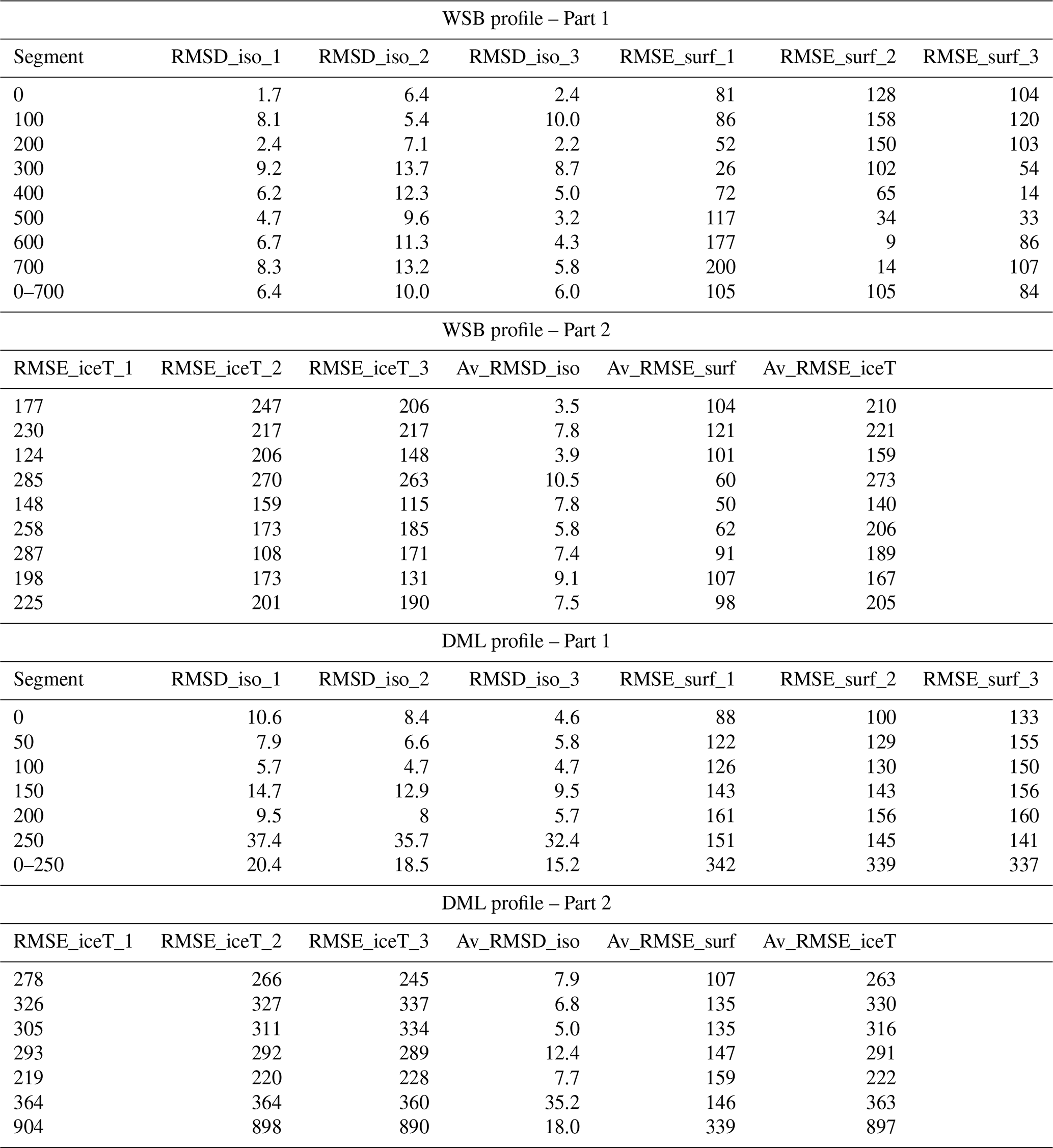
Over WSB, we traced nine IRHs spanning the Holocene and LIG (Fig. 2, Table 2). The depth and age of our IRHs match closely the depth and age of six isochrones from Winter et al. (2019) and Cavitte et al. (2021), with ages of 37.7 ± 0.5, 73.1 ± 1.2, 90.8 ± 1.4, 117.0 ± 1.3, 122.8 ± 1.0, and 128.4 ± 3.6 ka (Fig. 2c, e–i). The small age differences between our isochrones and those from Winter et al. (2019) and Cavitte et al. (2021) are attributed to the use of the newer version of the age–depth scale of Antarctic ice cores by Bouchet et al. (2023), as described in Sect. 2.2.3. Due to disruptions in the continuity of isochrones in the WSB radar data at the transition between the EDC-outbound lines and the main WSB grid covering the central part of the catchment (blue star in Fig. 1a), we were unable to connect many of the traced isochrones from EDC to the main grid with reasonable accuracy. As a result, and to obtain IRH coverage along the central grid-west to grid-east portion of the WSB grid (Fig. 1a), IRHs were also traced via their intersection with the age–depth profile at TALDICE ice core where they were dated (Fig. 2a–b, d). This included IRHs dated at 6.6 ± 0.1, 13.1 ± 0.3, and 64.1 ± 2.5 ka (Table 2). Unfortunately, this disruption in the continuity of internal layering in the upstream part of the main WSB grid and the lack of many crossovers in the radar data in this area hindered our ability to accurately connect isochrones between the EDC and TALDICE ice-core sites (Fig. 2). This problem has previously been reported elsewhere in East Antarctica (e.g., Cavitte et al., 2016) and points to the need for future surveys to provide enough crossovers in the radar data to ensure isochrones can be adequately traced between the divide and the fast-flowing sectors of the ice sheet.

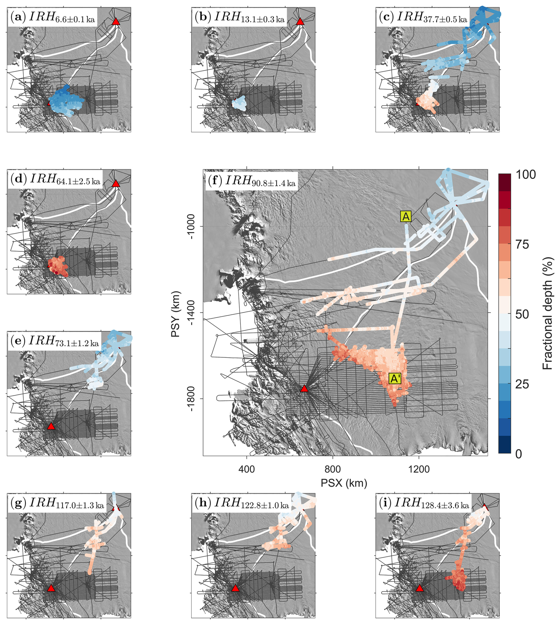
Figure 2 Spatial and vertical depth distribution (as a percentage of the local ice thickness) of each IRH traced over the legacy WSB data and connected to EDC and TALDICE ice cores (shallow depths in the ice column – blue; deeper depths in the ice column – red). The 90.8 ± 1.4 IRH coverage over WSB is shown more prominently in this figure as it is the one we use in the modelling section of this paper (see Sect. 3.2). The location of profile A-A' from Fig. 4a is depicted here again by the two yellow markers. The thin grey lines represent the full radar survey datasets onto which IRHs were traced, the red triangles represent the deep ice cores used to date the IRHs, and the white lines represent the main drainage basin boundaries (IMBIE, 2018). The background map is the 2014 MODIS mosaic of Antarctica (Haran et al., 2018).

When accounting for age uncertainties from this study, the isochrones traced and dated over WSB match closely the age of IRHs previously traced across other sectors of East Antarctica (Siegert, 2003; Leysinger Vieli et al., 2011; Beem et al., 2021; Wang et al., 2023; Franke et al., 2025b; Sanderson et al., 2024; Yan et al., 2025), an important finding for building a 3-D age–depth model of the ice sheet, as motivated by the SCAR AntArchitecture initiative (Bingham et al., 2025). The most extensive isochrone traced across WSB is the 90.8 ± 1.4 ka (Fig. 2f), which connects the EDC ice core site with the main WSB grid extensively, including as far grid-west as the foothills of the Transantarctic Mountains and in the upstream reaches of the Ninnis Glacier that drains part of the WSB catchment (Figs. 1a and 2f). Another prominent isochrone, dated at 128.4 ± 3.6 ka, connects EDC with the centre of the WSB grid, extending as far downstream (grid south) as the 90.8 ka IRH (Fig. 2i). This isochrone provides an important time marker, ideally dated to around the same time as the onset of the Last Interglacial (LIG; 130-115 ka before the present), and which can be combined with past geological evidence and model simulations that indicate substantial grounding line retreat and ice dynamical changes occurring in this area of East Antarctica during the LIG (Blackburn et al., 2020; Sutter et al., 2020; Crotti et al., 2022; Iizuka et al., 2023).

It is worth noting that the three deepest isochrones in the WSB catchment, and particularly the oldest IRH dated at 128.4 ka, vary spatially in their reflection strength, forming first a very clear reflector but quickly transitioning to a thick band of diffuse scattering in the BAS chirp data on approach to the main WSB grid from EDC. This diffuse reflector band for the oldest IRH is approximately 15 samples in the vertical range of the BAS PASIN radar system, which approximates to ∼ 50 m in the ice. We picked the upper part of this diffuse reflector where it was continuous, but lost it further grid-south where ice-surface speeds and thick ice make these reflectors difficult to interpret. Although uncertainties in both age and depth are greater for this deepest reflector, this IRH is crucial for assessing deep – and therefore old – ice in the catchment and for calibrating the ice-sheet model for this time period. We therefore accept a larger uncertainty for the deepest isochrone over WSB, of approximately ± 50 m, corresponding to ± 3.6 ka at EDC (Table 2), which is twice the uncertainty associated with the 127.8 ± 1.8 ka IRH in Cavitte et al. (2021). This uncertainty will be more appropriate in such areas where we pick this diffuse reflector band (i.e. in the downstream section of the WSB grid), but we expect a much smaller uncertainty of ∼ 1.8 ka in the upper part of the WSB survey grid and towards EDC due to the fact that the reflection is much more distinct and intersects Cavitte et al. (2021)'s IRH in several places with little difference in depth at those crossovers.

Figure 3 Spatial and vertical depth distribution of each IRH traced over the newly acquired DML data and connected to EMDL and Dome Fuji ice cores using legacy AWI data. As for Fig. 2f, the 91.0 ± 1.1 IRH coverage over DML is shown more prominently in this figure as it is the one we use in the modelling section of this paper (see Sect. 3.2). The location of profile B-B' from Fig. 4b is depicted here again by the two yellow markers. The items present on this figure are described in the caption of Fig. 2.

3.1.2 IRHs over DML

Over DML, we traced a total of seven IRHs across all survey lines, with ages from younger to older: 4.8 ± 0.6, 7.4 ± 0.8, 25.6 ± 0.1, 38.1 ± 0.1, 52.2 ± 0.1, 73.4 ± 0.9, and 91.0 ± 1.1 ka (Fig. 3 and Table 2).

Most IRHs are the exact same isochrones as traced previously by Franke et al. (2025b), and so we did not re-calculate the age and age uncertainties and relied on Franke et al. (2025b) for the dating of our IRHs. The only exceptions to the above is the second-shallowest and the deepest IRHs in our DML dataset, which differ slightly from those of Franke et al. (2025b). Our second-shallowest IRH, dated at 7.4 ± 0.8 ka sits slightly deeper in the ice than Franke et al. (2025b)'s 7.3 ± 0.8 ka IRH, and so we traced it to EDML for dating. We note, however, that these two closely spaced IRHs correspond to a couplet seen for several tens of kilometres on the CHARISO lines, but with the shallowest one fading away quickly to leave only one distinct isochrone which we traced here. This characteristic of being a couplet of two shallow isochrones, compounded with the fact that a couplet of similar age was also traced widely across the WAIS (Ashmore et al., 2020; Bodart et al., 2021) and found to correspond to strong peaks in acidity concentrations in the WAIS Divide ice core (Bodart et al., 2021), leads us to postulate that this set of isochrones may be a reliable widespread marker of a powerful volcanic eruption that may have left signatures across large swathes of the WAIS and EAIS. Similarly, our deepest IRH, dated at 91.0 ± 1.1 ka is the same as the IRH found around EDML ice core by Franke et al. (2025b), and is now traced across the divide connecting EDML and Dome Fuji ice cores (Fig. 3g).

Table 2 Depth and age statistics for all isochrones mapped on WSB and DML. Columns 3 and 4 are provided for all data points across both catchments, whereas column 5 refers to the mean depth at the respective ice core specified in column 8, averaged across a pre-defined radius around the ice cores (see Sect. 2.2.3). Columns 5–6 for the DML region are blank for IRH 1-6 as these were traced and dated by Franke et al. (2025b) (refer to their paper for these values). ^* For IRH 7 over DML, we provide the mean depth and mean depth uncertainty at Dome Fuji (DF) ice core, but the age and age uncertainty is the one provided by Franke et al. (2025b) at EDML.

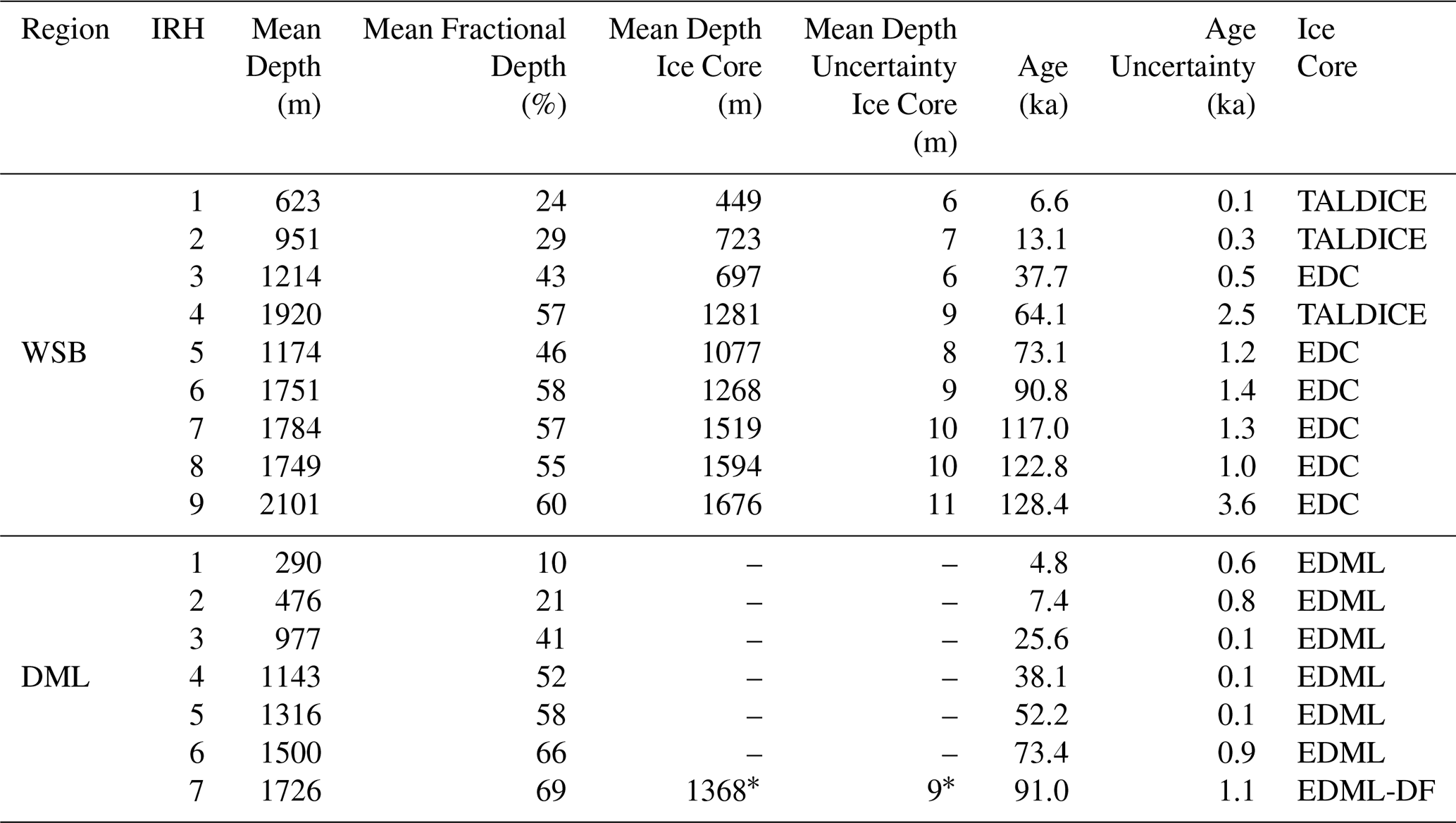
Over our new survey lines, we find that the four deepest IRHs (38.1, 52.2, 73.4, and 91.0 ka) extend much more downstream and across to the SRG ice stream than the shallowest IRHs which fade more rapidly away from the ice divide (Fig. 3d–g vs. a–c). Moreover, IRHs become heavily disrupted over faster-flowing ice downstream near where a subglacial mountain range constrains ice-stream flow through deep trenches on approach to the bluff onto which the PE station is located (Figs. 1b–3). As shown by Franke et al. (2025b), all the isochrones traced over DML correspond to the approximate age (when uncertainties are accounted for) of other previously traced and dated IRHs across both West and East Antarctica (e.g., Siegert, 2003; Siegert et al., 2004; Siegert and Payne, 2004; Leysinger Vieli et al., 2011; Steinhage et al., 2013; Muldoon et al., 2018; Ashmore et al., 2020; Beem et al., 2021; Bodart et al., 2021; Chung et al., 2023; Wang et al., 2023; Sanderson et al., 2024; Yan et al., 2025), and importantly, match the ages of major volcanic eruptions. Exemplifying this is the fact that we find over both WSB and DML three common IRHs (∼ 38, ∼ 73, and ∼ 91 ka) across both regions when age uncertainties are accounted for, despite both sectors being at opposite ends of East Antarctica with a distance of 2000 km separating Dome Fuji and EDC.

3.2 Data–model comparison

We now proceed to discuss the data-model comparison, focusing first on the modelling rationale and the key sets of model parameters that were used in our simulations. We then discuss the modelling results, which are presented in Fig. 4a for WSB and Fig. 4b for DML, as well as in Table C1.

3.2.1 Modelling rationale

It is important to note that here, we do not conduct an in-depth analysis of isochronal elevations and patterns for each time slice shown in Figs. 2–3, as is common for purely data-focused isochronal studies (e.g., Cavitte et al., 2016; Winter et al., 2019; Ashmore et al., 2020; Bodart et al., 2021; Franke et al., 2025b; Sanderson et al., 2023). This is because our main objectives are to (i) provide isochronal data tailored to ice-sheet modelling purposes, and (ii) exemplify the use of these datasets via comparison of individual isochronal transects with model simulations.

One way to demonstrate the usefulness of isochrones in constraining 3-D model simulations in off-divide locations – and to disentangle climatic imprints (e.g., surface mass balance variations) from dynamical or physics-based processes that the model does not accurately represent – is through the interrogation of multiple targeted isochrones dated at or near major climate transitions (e.g., Holocene, LGM, LIG) (MacGregor et al., 2015; Born and Robinson, 2021), or alternatively by examining single isochrones across large regions or long transects (Sutter et al., 2021).

Here, we focus on the latter and select a common isochrone which was traced and dated independently and which is present across large swathes of both WSB and DML. This isochrone, dated at 90.8 ± 1.4 ka over WSB (Fig. 2f) and 91.0 ± 1.1 ka over DML (Fig. 3g), is also a common isochrone found widely across other sectors of the EAIS (Winter et al., 2018; Beem et al., 2021; Sanderson et al., 2024; Franke et al., 2025b) and likely results from a large explosive volcanic event originating from Mt. Berlin (West Antarctica) that left tephra deposits in EDC and Dome Fuji ice cores at around the same time (Narcisi et al., 2006). We assume that this isochrone is the same reflection across both WSB and DML when uncertainties are considered, especially because it was consistently imaged by a series of radar systems across distant regions of the EAIS and dated at several ice cores, with the absolute age and age uncertainties reflecting the diversity in tracing, dating, and the multitude of datasets used (e.g., Table 1). For the sake of brevity, we will refer to this isochrone as the 91 ka isochrone for the remaining part of this paper.

Choosing to focus solely on this 91 ka isochrone is a deliberate choice, partly due to it being the most spatially extensive isochrone across both sectors, but also because it was deposited during a period when East Antarctica likely experienced broadly similar conditions across these two extensive sectors, in a phase of ice re-growth following the LIG retreat. Nonetheless, whilst we do not directly use the other 15 isochrones traced here in the modelling, we note that most of them were deliberately traced as they coincided either with major climatic transitions (i.e., LIG or Holocene) or with previously traced and independently dated isochrones from previous studies. This strategy facilitates their direct use in modelling studies, allowing models to target isochrones associated with key climatic events or to simulate isochrones of a specific age that can be consistently compared across large spatial scales, thus highlighting the value of tracing isochrones of equivalent age. Building on this foundation, more comprehensive data-model comparisons, based on large-scale regional modelling ensembles constrained by the full suite of isochrones presented here, will be undertaken in forthcoming work, and we encourage others to make use of these datasets in their own modelling applications.

To best evaluate how well the model reproduces the observed isochrone, we ran three simulations on a regional domains across WSB and DML by slightly modifying the precipitation scaling which governs the relationship between surface temperature change and precipitation change, and the PISM-specific till effective pressure parameter which governs how much of the overburden pressure from the ice load is transferred to the subglacial till to drain excess water from the sediment column (Bueler and van Pelt, 2015), thereby modulating the effective pressure (Fig. 4).

Whilst the precipitation scaling controls Surface Mass Balance (SMB), which in East Antarctica is dominated by net accumulation of snow and minimal surface melt, the till effective pressure influences sliding over the bed via its interaction with the substrate underneath the ice. The selection of these two parameters was thus made to illustrate the imprint of SMB and basal ice flow on the elevations of isochrones via a small (but commonly used) subset of the large parameter space available to ice-sheet models and climate forcing choices (i.e., Albrecht et al., 2020). We tested values for the precipitation scaling ranging from 5 %–11 % and for the till effective pressure from 0.023–0.03 (Fig. 4). The first range of values is informed from reconstructions of precipitation scaling at ice cores across Antarctica (particularly the low-end of this range, e.g., Frieler et al. (2015); Fudge et al. (2016)) and testing of values slightly outside of these reconstructions that provide a best-fit in isochrone elevations (i.e., the higher-end of this range). The second parameter is a refined range of values that produces acceptable present-day offsets between modelled and observed surfaces within a much wider range of possible values. We note that many other parameters can also influence the present-day offsets in surface elevations and the mismatch in isochrones; however, mismatches in isochrone elevations across drainage basins influenced both by surface mass balance changes as well as ice dynamics are particularly driven by these two PISM parameters whilst at the same time providing similar surface elevation offsets, thus making them ideal for our experiments.

3.2.2 Comparison between the observed and modelled 91 ka isochrone across WSB and DML regions

On Fig. 4, we show two long profiles across WSB (740 km) and DML (290 km) where the 91 ka isochrone is present and crosses two ice-dynamically diverse regions: (1) the stable ice divide where the position of the isochrone in the ice is primarily the result of SMB variations and changes in GHF (Sutter et al., 2021), and (2) the faster-flowing areas of the ice sheet away from the ice-divide where ice dynamical processes such as ice deforming over subglacial bedrock at relatively fast speeds is common and where the geometry of isochrones can become heavily distorted (e.g., Catania et al., 2005).

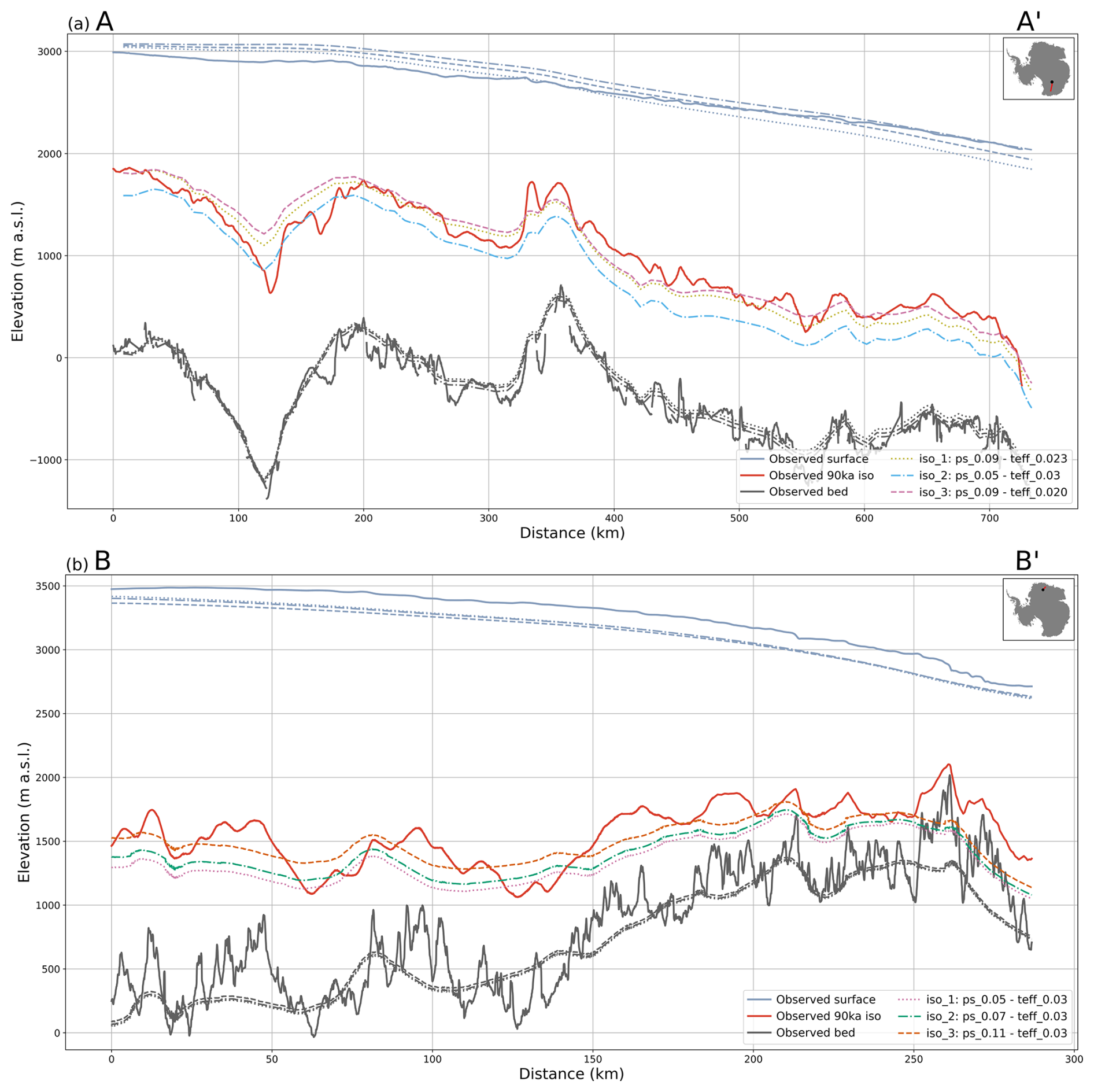
Figure 4 Comparison of the 91 ka isochrone from observations and model simulations generated in this study, along profiles A-A' (WSB, a) and B-B' (DML, b) crossing the ice divide (start) to fast-flowing ice downstream (end) (exact locations shown in Fig. 1). The solid lines represent the observed (i.e., picked) ice surface, bed and isochrone elevations from the radar data. The non-solid lines (dashed, dashed-dotted, and dotted) represent three simulations that were ran to simulate an accurate paleo-evolution of the two catchments. For each observed surface, bed and isochrone from the radar, we show the three corresponding modelled surfaces, isochrones, and beds which were transiently simulated by the model. The abbreviations “ps” and “teff” in the plot legends refer respectively to the precipitation scaling and till effective pressure parameters mentioned in Sect. 3.2.1), and the “iso” numbers (ranging from 1 to 3) preceding these refer to each of the three simulations matching the specific parameter values for “ps” and “teff” in the legends. For simplicity, we refer to each of these simulations in the text and in Table C1 using this “iso” numbering abbreviation.

Often, ice-sheet modelling studies that run long paleo-simulations on glacial to interglacial timescales are tuned to present ice-sheet states from observations (i.e., modern ice-sheet conditions such as ice thickness and ice-flow speeds) and past ice-sheet states from paleo-reconstructions (i.e., grounding-line reconstruction from sediment cores). This calibration ensures that the ice-sheet model accurately represents known processes well and evolves following realistic paleo-conditions (Albrecht et al., 2020). Once the ice-sheet model is initialized to match such present and past ice-sheet states, it is typically run for several thousand to hundreds of thousands of years from past to present day, under the assumption that, because it is calibrated to modern ice-sheet conditions and sparse paleo-information, its transient evolution provides a reliable representation of the past evolution of the ice sheet. Unfortunately, an acceptable match to present day and sparse paleo-benchmark datasets does not guarantee a proper representation of internal ice flow as illustrated in Fig. 4, which shows close match to modern ice-sheet configuration along a radar transect (i.e., ice-sheet surface), while at the same time highlighting considerable deviations to the proxy record (in this case from the observed isochrone) in both regions. In this context, a mismatch between the modelled and observed isochrones potentially indicates over-tuning of the ice-sheet model, something which is difficult to identify via simple comparisons with current ice geometries or sparse paleo-reconstructions.

A striking observation is that relying on interpolated gridded products such as Bedmap3 (as used here) or other gridded products (e.g., Bedmachine, Morlighem et al., 2020) as appropriate boundary conditions to run ice-sheet models can be problematic, particularly in areas with sparse underlying data used to generate the gridded product. This is exemplified in Fig. 4b where the observed bed imaged in the newly acquired radar data (and which was not included in the latest iteration of the Bedmap gridding product) differs substantially from the modelled beds due to the lack of reliable Bedmap3 data in the area surrounding the new CHARISO lines (see also Fig. B1). This is particularly striking in the last ∼ 40 km of the profile where a subglacial mountain imaged by the radar is not present in the modelled beds, resulting in the modelled isochrones cutting through the observed bed. This section of the profile is also where we observed one of the largest differences between observed and modelled isochrones (Fig. 4b; Table C1). This exemplifies the utility of using isochrones as a data-benchmark for ice-sheet modelling to investigate both the minimum amount of bedrock offset that is required to produce such contrasting isochronal elevations and to rapidly identify areas where the modelling results can be least trusted.

Closer to the ice divide, the modelled isochrones are primarily controlled by SMB, which is where the largest difference in simulations employing different precipitation scaling is seen, particularly on the DML profile where the difference in modelled isochronal elevations is greater near the divide than near the end of the profile in a compressive flank-flow regime (Fig. 4b). It is at the end of the profile that the difference in isochronal elevations between the different simulations is reduced, with none of the simulations able to match the observed isochrone as a result of the unrealistic representation of the modelled bed compared with the observed bed. We also note that selecting a higher precipitation scaling than what reconstructions at ice-cores suggest (e.g., Frieler et al., 2015) appears to improve the agreement between the average elevation of the observed and modelled isochrone close to the ice divide, whereas reducing this value means that the modelled isochrone is too low in the ice column. This result was also previously highlighted in Sutter et al. (2021), where a higher precipitation scaling provided a better match with the local isochronal stratigraphy, likely pointing to the fact that a uniform precipitation scaling across the region is unlikely to correctly represent the variable conditions away from ice-divide locations.

Similarly over WSB (Fig. 4a), the difference between each simulation is slightly larger closer to the ice divide, owing to the strong control of SMB on the modelled isochrone elevations there, whereas this difference reduces further downstream. While the two modelled isochrones iso1 and iso3 appear to better match the observed isochrone in the first half of the profile, ice dynamical processes downstream result in them being situated too low in the ice column compared with the observed isochrone. This is a problem that has previously been identified in deep marine basins below sea level, where the basal drag in the model is designed to be linearly reduced as bedrock elevation decreases, leading to faster sliding (Sutter et al., 2021). Combined with a model resolution of 8 km², which is relatively high for transient paleo-modelling but still coarse compared to the 500 m Bedmap3 grid, the smoothing of bedrock obstacles and reduction in basal friction at this scale likely contributes to an overall drawdown of modelled isochrones relative to observations in this sector.

For an acceptable level of differences in modern surface elevation and ice thickness between the modelled elevations (last time step in the model) and observations (from radar or gridded products), we find that isochrones can differ more substantially and at times in contradictory fashion, pointing to the fact that a good match with modern ice surface elevations and ice thickness does not guarantee a good match in isochrone elevation. This is illustrated in Fig. 4a over WSB where the mean Root Mean Square Error (RMSE) for surface elevations and ice thickness along the entire length of the profile is 98 and 205 m, respectively, whereas the mean Root Mean Square Difference (RMSD; with reference to the local ice thickness, see Sutter et al., 2021) for all modelled isochrone elevations is 7.5 % (equivalent to an RMSE in isochrone elevations of 221 m) across all three isochrones for the entire profile (6.4 % or 190 m RMSE for iso1, 10.0 % or 286 m RMSE for iso2, and 6.0 % or 187 m RMSE for iso3; Table C1). It is important to note, that these RMSE values further improve when only considering portions of the transect where the gridded bedrock at model resolution fits the observed bedrock reasonably well. When calculating RMSE in surface elevation and ice thickness for each 100 km segment along the profile, we find that the best matches for surface elevation (4 out of 7 segments) and ice thickness (6 out of 7) come from both the best (iso3) and worst (iso2) isochrone RMSD values (Table C1). This suggests that, for this particular profile, a good agreement with observed surface elevation and ice thickness does not necessarily translate to an accurate transient model evolution. In fact, a simple tweak of just two model parameters (in this case precipitation scaling and till effective pressure between iso3 and iso2) can nearly double the RMSD for this isochrone, while still maintaining a good match with surface elevation and ice thickness, illustrating how sensitive the model’s temporal evolution is to small parameter changes.

A similar pattern is found over DML (Fig. 4b; Table C1) where the best match in surface elevations (4 out of 6 segments) and ice thickness (3 out of 6 segments) come from the simulation where the isochrone has the highest RMSD value (iso1; 20.4 % or 359 m RMSE-equivalent) and thus the poorest match to isochrone observations. This contrasts with only $\mathrm{1}/\mathrm{6}$ and $\mathrm{3}/\mathrm{6}$ of all segments for surface elevation and ice thickness, respectively arising from the simulation where the isochrone has the lowest RMSD value (iso3; 15.2 % or 285 m RMSE-equivalent) and thus the best match in isochrone observations (Table C1). We note that a precipitation scaling of 11 % as employed in the simulation that produced iso3 is likely an overestimate of the average precipitation scaling calculated for the high plateau areas of the East Antarctic Ice Sheet (including EDML), where the mean continental-scale value was estimated to be ≈ 5 ± 1 % K⁻¹ (Frieler et al., 2015), although recent evidence suggests that LGM temperature was likely less cold than previously estimated, implying higher precipitation across the EAIS (Buizert et al., 2021). The reason for a high-end precipitation scaling reducing the overall isochronal mismatch over this profile is likely two-fold: (i) low precipitation scaling are potentially more accurate over high-elevation ice divide locations than in off-divide areas, and (ii) the misrepresentation of the true bedrock topography in the boundary conditions used to run the model compared with our newly acquired radar data, which results in unrealistic simulations of isochronal elevations along this profile. A high-precipitation scaling can compensate for this mismatch in bedrock elevations but is not necessarily the most adequate. This illustrates effectively that even though isochrones are a powerful tool for model calibration, they should only be applied where the model can represent the observed bedrock topography to a reasonable degree.

What is also notable in the DML transect is the low sensitivity of the surface elevation mismatch at present day compared with correspondingly strong offsets between the modelled and observed isochrones. Ultimately, parameters and forcing choices are key in optimising modelled isochrone geometry while preserving a good match with present day ice-sheet observations. The example shown here highlights that past SMB variations substantially modulate isochrone geometry while affecting the present-day fit of the ice sheet only moderately. Choosing proper sliding laws and associated parameterisation for isochrone geometry is much more challenging, as already small grounding line mismatches can lead to large model deviations from the observed present-day ice-sheet geometry. As it only makes sense to compare isochrone geometries if the modelled present day ice sheet matches observations, the operating space in ice dynamic parameters is much more limited.

We conclude that whilst the simulations with the highest precipitation scaling produce the best match in isochronal elevation along these two profiles, this is not necessarily associated with the simulations which exhibit the best match in surface elevations or ice thickness. However, since thickness deviations are acceptable for the experiments considered here (i.e., compared to other present-day spin ups in the ISMIP6 intercomparison exercise, Seroussi et al., 2020), we can extract several key messages from this analysis: (i) ice-sheet models can relatively accurately simulate ice-sheet evolution through long time-scales at 8 km resolution, as illustrated by the relatively good match of data and model along these two profiles and across all three simulations (where mean RMSD in isochrone elevations in the well-constrained WSB profile ranges between 6.0 and 10.0 %; equivalent to an RMSE in isochrone elevations of between 187 and 286 m). This is particularly encouraging considering that this isochrone is relatively deep in the ice column and crosses several boundaries where different processes (SMB vs ice dynamics) dominate and where ice-flow transitions from slow to fast flowing; (ii) the underlying boundary conditions used to constrain the ice-sheet model (i.e., here Bedmap3) can significantly affect the transient evolution of the simulations, particularly in areas where strong interpolation in the underlying data product was required due to the lack of nearby bed elevation data from radars. This has the effect of strongly misrepresenting the isochronal architecture there, as exemplified towards the end of the DML profile where mean RMSD values for the isochrones exceed 35 % in the last ∼ 40 km (equivalent an RMSE of 399 m), leading in turn to a misrepresentation of the mean RMSD value in isochrone elevations for the entire profile (i.e., 18.0 %; Table C1); and (iii) the use of isochrones as spatially extensive paleo-proxies must form a greater part in constraining ice-sheet modelling results away from stable ice divides to improve simulations and avoid biases, particularly in areas where little other proxy records such as grounding-line reconstructions (Bentley et al., 2014), ice-elevation change reconstructions (Johnson et al., 2021), or other paleo-proxies (Lecavalier and Tarasov, 2025) exists. This is particularly relevant when refining ice-sheet model parameters, as simply tuning an ice-sheet model to modern ice-sheet states does not guarantee a realistic transiently-calibrated ice-sheet model simulation.

4 Conclusions

Using both legacy radar data acquired over the Wilkes Subglacial Basin and newly acquired radar data over Dronning Maud Land, and the 3-D thermo-mechanically coupled PISM ice-sheet model, we showed that newly traced and dated radar isochrones present at locations away from the stable ice divide of East Antarctica can be extremely useful at assessing the model's ability to transiently simulate the evolution of the ice sheet. Alongside this paper, we also released two extensive datasets of isochrones (16 in total) tailored to ice-sheet modelling. These datasets span the Holocene and Last Interglacial (∼ 4.8–128.4 ka) over both investigated East Antarctic sectors and can be used for further (and more detailed) assessments of ice-sheet models' ability to accurately model the transient evolution of Antarctica. Of the 16 isochrones traced here, 13 correspond – within uncertainties – to previously traced and dated isochrones across both East and West Antarctica. Notably, despite the two sectors being at opposite ends of East Antarctica and separated by a distance of ∼ 2000 km, three common isochrones (∼ 38, ∼ 73, and ∼ 91 ka) are identified across both regions, with the ∼ 91 ka isochrone exhibiting the greatest spatial extent over both WSB and DML. Using this ubiquitous ∼ 91 ka isochrone in the model, we highlighted that a relatively good match between observed and modelled surface elevation and ice thickness does not necessarily correspond to the best match in isochronal elevations, pointing to the need for increased integration of isochrones in ice-sheet models, particularly in areas far from the stable ice divide where ice flow is faster and ice-sheet models preform less well. This study exemplifies the need to include further isochrones into ice-sheet models as an additional proxy to currently used tuning targets, such as modern ice thickness and ice-flow speeds, or key paleo-climate snapshots.

Appendix A: IRHs crossover-points analysis

In order to assess the accuracy of the IRH tracing across the wider WSB and DML regions, we performed a crossover-point analysis on all the IRHs traced in this study (Figs. A1–A2). For this analysis, we extracted all IRH points that fell within 30 m of a crossover point between two survey flight lines and calculated the depth difference of corresponding IRHs of the same age. Overall, crossover error is lesser over DML than WSB due to the use of newer radar systems in the former and a consistent processing applied to the radar data (Fig.  A2), with a median depth difference ranging from 1 to 8 m, which is well within the uncertainty range of the radar system and assumptions made regarding the electromagnetic wave speed in ice. Comparatively, over WSB, where we used data originating from four very different radar systems used between 2005 and 2020 (Table 1), and where data were acquired using different orientations to ice flow, the median depth differences ranged from 3 to 18 m (Fig. A1). Crossover error in WSB is typically greater for older IRHs (Fig. A1d, f–g, and i) where the IRHs transitioned from specular to diffuse and resulted in a thick layer package further downstream from the stable ice divide.

Figure A1 Crossover differences in IRH depths across the WSB radar lines. The median line is shown in red and the 1st and 3rd quartiles are shown as dashed lines.

Figure A2 Crossover differences in IRH depths across the DML radar lines. The median line is shown in red and the 1^st and 3rd quartiles are shown as dashed lines.

Appendix B: Bedmap3 bed uncertainty in the vicinity of the newly acquired CHARISO lines in DML

Figure B1 Bed uncertainty from the Bedmap3 dataset over DML, where dark grey lines represent the underlying data used to grid the final data product, and the light gray spacing represents gaps between known survey lines where the interpolation is conducted. Overlaid on top are the new CHARISO radar lines acquired as part of this paper (and which were not integrated in the latest iteration of the Bedmap gridding product), and in yellow the profile B-B' from Fig. 4b, with the last ∼ 40 km circled in red.

Appendix C: Differences in elevations between modelled and observed surfaces across the WSB and DML profiles

Table C1 Values for RMSD (91 ka isochrone elevations; in %) and RMSE (surface elevations or ice thicknesses; in metres) between observed and modelled surfaces, calculated for each of the three simulations shown in Fig. 4 for 100 (WSB) or 50 (DML) km segments, as well as for the entire length of the profile (last row). “Av” stands for average, “surf” for surface elevation, and “iceT” for ice thickness.