Reconstructing ice phenology of a lake with complex surface cover: a case study of Lake Ulansu during 1941–2023

Lake ice phenology plays a critical role in determining the hydrological and biogeochemical dynamics of catchments and regional climates. Lakes with complex shorelines and abundant aquatic vegetation are challenging for retrieving lake ice phenology via remote sensing data, primarily because of mixed pixels containing plants, land, and ice. To address this challenge, a new double-threshold moving t-test (DMTT) algorithm, which uses Scanning Multichannel Microwave Radiometer (SMMR) and Special Sensor Microwave/Imager–Special Sensor Microwave Imager/Sounder (SSM/I–SSMIS) sensor-derived brightness temperature data at a 3.125 km resolution and long-term ERA5 data, was applied to capture the ice phenology of Lake Ulansu from 1979 to 2023. Compared with the previous moving t-test algorithm, the new DMTT algorithm employs air temperature time series to assist in determining abrupt change points and uses two distinct thresholds to calculate the freeze-up start (FUS) and break-up end (BUE) dates. This method effectively improved the detection of ice information for mixed pixels. Furthermore, we extended Lake Ulansu's ice phenology back to 1941 via a random forest (RF) model. The reconstructed ice phenology from 1941 to 2023 indicated that Lake Ulansu had average FUS and BUE dates of 15 ± 5 November and 25 ± 6 March, respectively, with an average ice cover duration (ICD) of 130 ± 8 d. Over the last 4 decades, the ICD has shortened by an average of 22 d. Air temperature was the primary impact factor, accounting for 56.5 % and 67.3 % of the variations in the FUS and BUE dates, respectively. We reconstructed, for the first time, the longest ice phenology over a large shallow lake with complex surface cover. We argue that DMTT can be effectively applied to retrieve ice phenology for other similar lakes, which has not been fully explored worldwide.

1 Introduction

Global lake ice loss, a notable indicator of climate change (Kang et al., 2012; Li et al., 2022), profoundly affects Earth's climate system and the ecological dynamics of lake environments (Leppäranta et al., 2020; Yang et al., 2023). Lake ice regulates water temperature, light availability, and nutrient circulation, which are crucial for the ecological environment (Latifovic and Pouliot, 2007; Wu et al., 2022). Many studies have evaluated lake ice phenology trends in the Northern Hemisphere (Mishra et al., 2011; Sharma et al., 2019; Woolway et al., 2020), but shallow and vegetated lakes remain largely unexplored owing to their lack of long-term observational data. These lakes are more sensitive to climate change than deep lakes are because of their low heat capacity (Ambrosetti and Barbanti, 1999), which makes them more responsive to temperature fluctuations. A shortened ice-covered season leads to a longer period of open water, enhancing conditions for algal bloom growth and potentially causing ecological imbalances (Duan et al., 2012). Ice phenology data from such shallow lakes are crucial for understanding how temperature fluctuations influence water stratification, nutrient availability, and the biological rhythms of aquatic organisms (Sharma et al., 2021; Smits et al., 2021). This knowledge is vital for refining climate models and enhancing the accuracy of weather predictions, thereby assisting in the management and conservation of freshwater resources in a changing climate (Hampton et al., 2017; Yang et al., 2020b).

In situ observations provide a wealth of information on ice phenology (Benson et al., 2011; Yang et al., 2020a). However, due to environmental and logistical constraints, sustained manual monitoring is challenging (Jewson et al., 2009). Owing to their broader temporal and spatial monitoring capabilities, remote sensing data have been widely used in the study of lake ice phenology (Wang et al., 2021; Wu et al., 2022). For example, the MODIS Terra and Aqua products, specifically MOD10A1 and MYD10A1, were utilized to determine lake ice phenology across the Tibetan Plateau from 2001 to 2017 (Cai et al., 2019). Optical satellites offer data with higher spatiotemporal resolution, but they depend on solar energy reflected from Earth's surface, making them susceptible to cloud cover and lighting conditions (Murfitt and Duguay, 2021). In contrast to optical remote sensing, microwave remote sensing allows for monitoring of Earth's surface under most weather conditions (Nunziata et al., 2021). Active microwave remote sensing is utilized primarily for extracting ice phenology data from large waterbodies because of its relatively low (>10 d) temporal resolution (Antonova et al., 2016; Howell et al., 2009). This is because, in these lakes, the phase transition between water and ice takes more time.

Passive microwave remote sensing provides data with long temporal coverage and frequent revisit times, although it offers coarse spatial resolution. These characteristics make it particularly suitable for large lake ice phenology detection (Kang et al., 2012; Su et al., 2021). Additionally, a common challenge in this method is the use of mixed pixels. These are pixels that contain multiple surface types, such as water, vegetation, and land, which are especially common around complex shorelines (Bellerby et al., 1998). To mitigate the impact of mixed pixels, buffer zones are typically implemented within passive microwave remote sensing technology, effectively shrinking the shoreline when extracting pixel information (Cai et al., 2022). The latest Calibrated Enhanced-Resolution Passive Microwave Daily EASE-Grid 2.0 Brightness Temperature (CETB) data offer multisource sensor-derived brightness temperature data from 1979 to the present, with a spatial resolution as high as 3.125 km. While this advancement significantly improves the monitoring capabilities of Earth's surface (Johnson et al., 2020), it still poses challenges in accurately capturing data for small lakes or lakes with complex shorelines due to mixed pixels.

In addition, if long-term lake ice phenology records are desired, satellite remote sensing can also provide training datasets for machine learning (Wu et al., 2021; Xu et al., 2024). For example, Ruan et al. (2020) presented a practical machine learning application in which a random forest model was used to forecast the ice phenology of lakes on the Tibetan Plateau until 2099. The ice phenology history derived from passive microwave remote sensing and Coupled Model Intercomparison Project Phase 6 (CMIP6) meteorological data was employed here as inputs. The success of this application largely depends on the quality of the training data, requiring not only accuracy but also a long temporal record that captures the variability in environmental conditions. To ensure the robustness of the model, it is critical to integrate diverse meteorological factors, such as air temperature, wind speed, and precipitation, along with ice phenology data, as these factors significantly influence lake ice. Furthermore, developing effective machine learning models that can address the complexities of lakes with various surface characteristics is essential.

This study uses Lake Ulansu as an example; this lake is the largest aquatic-plant-dominated shallow lake in northwestern China and is characterized by its rich aquatic vegetation and complex shoreline. The objective of this study was to develop an automated algorithm that overcomes the mixed-pixel challenges posed by rich aquatic vegetation and complex shorelines, thus enabling accurate classification of ice and water states and obtaining reliable ice phenology data for long-term reconstructions. Specifically, our research strategy was composed of the following steps. (1) A new algorithm was developed to classify the ice and water states on the lake surface in brightness temperature data from the Scanning Multichannel Microwave Radiometer (SMMR) and Special Sensor Microwave/Imager–Special Sensor Microwave Imager/Sounder (SSM/I–SSMIS) sensors for the period 1979–2023. (2) A random forest model was trained using the results in step 1 to reconstruct the ice phenology from 1941 to 1978. (3) The meteorological impact on the ice phenology of Lake Ulansu from 1941 to 2023 was analyzed to explore the key drivers of its variations.

2 Study area

Lake Ulansu (40°46^′–41°7^′ N, 108°41^′–108°58^′ E) is situated on the eastern side of the Hetao Basin in northern China (Fig. 1a). The lake covers an area of 306 km². It has an elevation of approximately 1050 m; a shoreline perimeter of approximately 140 km; and a north–south width ranging from 35 to 45 km, whereas its east–west width is narrower, at approximately 5 to 10 km. The water depth varies from 0.5 to 3 m, with an average depth of 1.6 m, indicating that the lake is a typical shallow lake. As an important water resource in the Hetao Basin, Lake Ulansu profoundly impacts local agriculture, irrigation, residents' livelihoods, and the regional climate (Guo et al., 2008; Li et al., 2020). The lake is rich in aquatic vegetation (Fig. 1c), which accounts for approximately 60 % of the lake area (i.e., 180 km²). The transpiration of reeds and lake evaporation result in considerable water loss, with an annual evaporation of approximately 2300 mm (White et al., 2020). Precipitation in the lake area primarily occurs during the summer, with an annual precipitation of approximately 220 mm (Sun et al., 2011). The lake's water depth and volume are regulated primarily during the summer through water diversion from the Yellow River, with minimal surface water inflow or outflow occurring during the winter (Huang et al., 2022). The Hetao Basin has an annual average air temperature of approximately 7.0 °C, with average air temperatures in January and July reaching −10.1 and 23.8 °C, respectively (White et al., 2020). Typically, the freeze-up start (FUS) date occurs in November, and the break-up end (BUE) date occurs in March, with an average ice cover duration (ICD) of 127 d from 2013–2022 (Huo et al., 2022). During mid-winter, the ice cover reaches a maximum thickness of 0.4 to 0.6 m (Huang et al., 2022), providing a crucial platform for local transportation and recreational activities. In this study, each hydrological year (HY) is defined as beginning on 1 August and ending on 31 July of the following year. For example, HY2022 spans from 1 August 2021 to 31 July 2022.

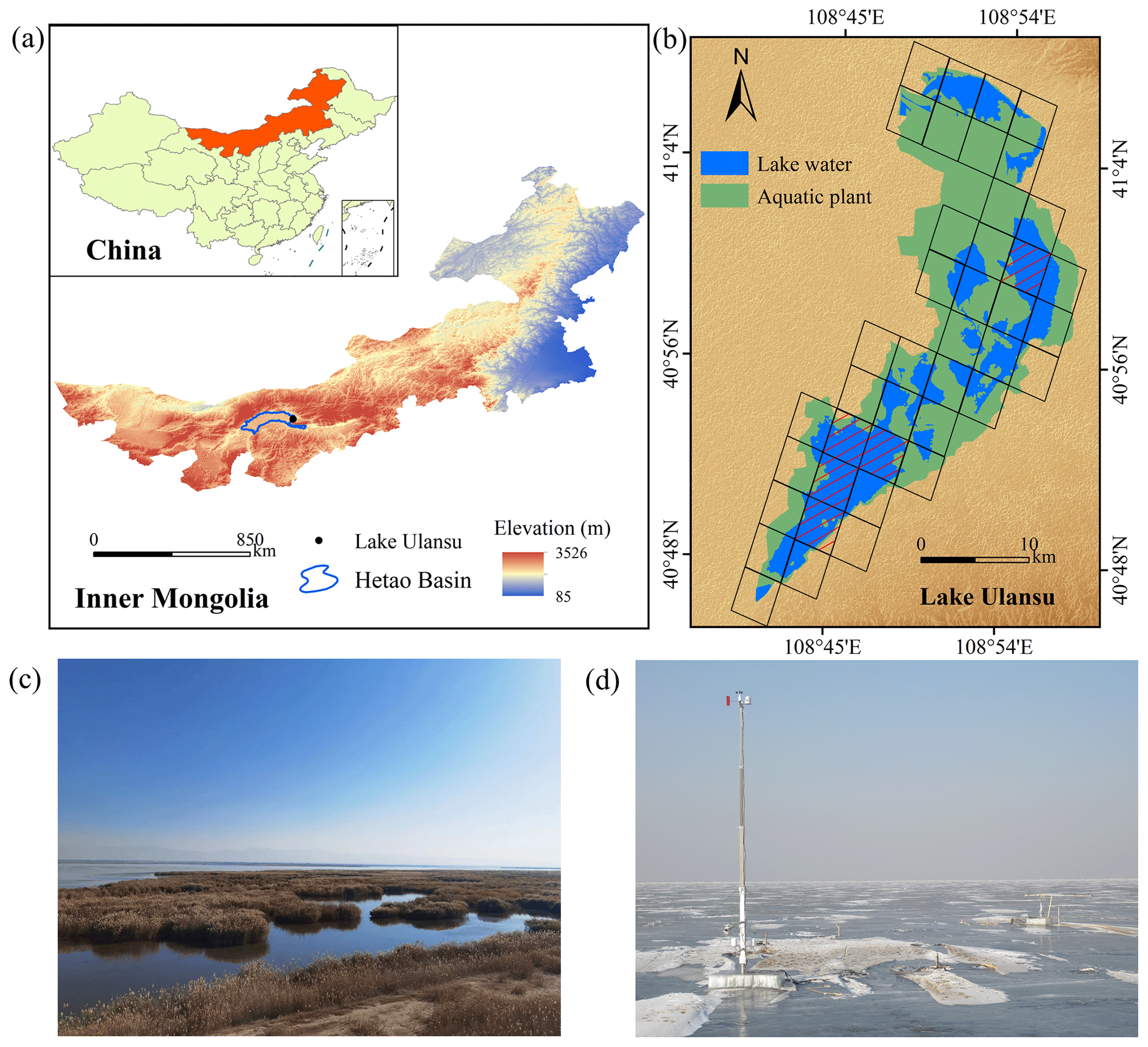
Figure 1 (a) Geographical context and elevation profile of Lake Ulansu within the Hetao Basin, Inner Mongolia. (b) CETB data grids with shaded areas representing brightness temperature pixels selected for Lake Ulansu surface identification. (c) Photographic depiction of aquatic reeds within Lake Ulansu. (d) On-ice instrumentation for field observations (Cao et al., 2021).

3 Data and methods

Three datasets and two algorithms were used in this study, as shown in the flowchart (Fig. 2). First, the double-threshold moving t-test algorithm and ERA5 air temperature data (1979 to 2023) were used to detect abrupt change points in the brightness temperature series from the CETB dataset. These points help classify brightness temperature pixels as ice or water states, allowing for the determination of the FUS and BUE dates for Lake Ulansu from 1979 to 2023. These dates were also validated by ice phenology data obtained from optical satellite data (MODIS, Landsat, and Sentinel-2) from 2000 to 2023. Next, meteorological data from ERA5 for the period from 1979 to 2023, along with ice phenology data derived from brightness temperature data, were used to train a random forest model. We subsequently input the ERA5 data from 1941 to 1978 into the trained random forest model to obtain historical ice phenology data for Lake Ulansu from 1941 to 1978.

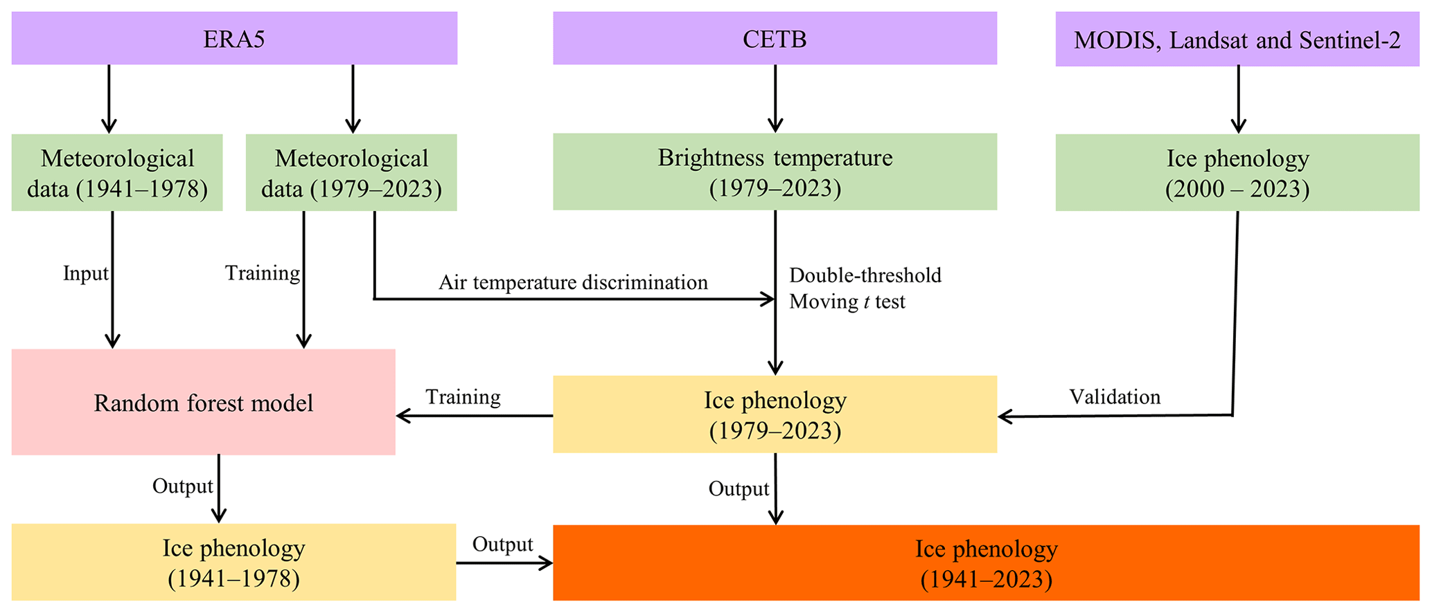
Figure 2 Reconstruction of the ice phenology of Lake Ulansu (1941–2023) based on ERA5, CETB, and optical satellite data via the double-threshold moving t-test algorithm and random forest model.

3.1 Data

3.1.1 Brightness temperature data

In this study, we used Calibrated Enhanced-Resolution Passive Microwave Daily EASE-Grid 2.0 Brightness Temperature (CETB) data at 37 GHz horizontally polarized with a high spatial resolution of 3.125 km provided by the National Snow and Ice Data Center (NSIDC). The CETB data include an abundance of microwave radiation brightness temperature (T_b) data, facilitating the investigation of Earth's surface characteristics. The CETB data were obtained from various satellite sensors with coarse spatial resolutions (∼ 25 km), including SMMR on Nimbus 7, SSM/I and SSMIS on the Defense Meteorological Satellite Program (DMSP) satellite series, and the Advanced Microwave Scanning Radiometer for EOS (Earth Observing System) (AMSR-E) on Aqua (Brodzik et al., 2016). For our specific analysis, we used only data from SMMR on Nimbus 7; SSM/I on the DMSP F08, F10, F11, F13, and F14 satellites; and SSMIS on the DMSP F16 satellite. CETB data boast high spatial resolution and comprehensive record features. The microwave radiation T_b data were collected from various channels and time intervals and were stored with grid spacings ranging from 3.125 to 25 km. The CETB grid employs the “drop-in-the-bucket” average algorithm to map essential location data onto output grid units, resulting in T_b data with a 25 km resolution. The resolution was subsequently enhanced via the radiometer version of the scatterometer image reconstruction (rSIR) algorithm, which yielded T_b data with resolutions ranging from 3.125 to 12.5 km. Owing to the narrow and irregular shoreline of Lake Ulansu, high-spatial-resolution T_b data were essential. Furthermore, the CETB data exhibited a relatively coarse spatial resolution of 6.25 to 12.5 km at frequencies below 30 GHz (Brodzik et al., 2016), with higher frequencies (near 90 GHz) being more susceptible to weather effects (Ivanova et al., 2015).

3.1.2 Optical satellite data

In this study, we use ice phenology data for Lake Ulansu from 2000 to 2023 obtained from optical satellites by Huo et al. (2022) to validate the ice phenology results derived from T_b data. These optical satellite data include red band reflectances from the MOD09GQ and MYD09GQ datasets, cloud information from the state_1km_1 parameter of the MOD09GA and MYD09GA datasets, and the Landsat and Sentinel-2 datasets. The single-band threshold method classifies red band reflectances into water and ice pixels. Compared with higher-spatial-resolution Landsat and Sentinel-2 datasets, the dynamic threshold method aims to determine the optimal threshold for distinguishing ice and water pixels (Zhang and Pavelsky, 2019). Additionally, the spatiotemporal continuity of MODIS datasets is used to fill in real pixels under clouds, resulting in more accurate pixel classification. By employing thresholds of 20 % and 80 % to differentiate the proportions of ice and water pixels in the total pixel count, it was possible to calculate the FUS and BUE dates. The ICD was then derived from the difference between these two dates. Owing to the higher spatiotemporal resolution of the MODIS products, these three ice phenology data points agreed with field observations (Huo et al., 2022).

3.1.3 Meteorological data

In this study, the ERA5 meteorological dataset, which was provided by the European Centre for Medium-Range Weather Forecasts (ECMWF), was utilized for comprehensive analysis. ERA5 is the latest reanalysis dataset that integrates model data with global observational data to produce a consistent dataset with a spatial resolution of 0.25° × 0.25° and a temporal resolution of 1 h. In this study, a collection of ERA5 hourly data at single levels from 1940 to the present was chosen. The selected meteorological variables included air temperature, wind speed, incident solar radiation, and precipitation (including rainfall and snowfall), which spanned from 1941 to 2023. Although meteorological stations are scarce in the Hetao Basin, a comprehensive evaluation of the suitability of ERA5 data for Lake Ulansu is still necessary. Detailed comparisons of air temperature, wind speed, and incident solar radiation against field observations from 2016 to 2018 and from 2022 to 2023 are provided in Appendix A, which underscores the robustness of the ERA5 data for climatological studies in this region.

3.2 Methods

3.2.1 Identification of lake surface states

In this study, the ice phenology from 1979 to 2023 was determined by the brightness temperature (T_b) of the lake surface because T_b changes considerably when a phase change occurs on the lake water surface (Su et al., 2021), providing a clear reference for determining the onset and end of the ice period. However, owing to the complex shape of the Lake Ulansu shoreline, which is characterized by its narrow form, pixels encompass not only water but also aquatic vegetation and land. As a result, five T_b grids with a proportion of lake water greater than 0.70 were selected to represent the status of the lake surface (Fig. 1b). Figure 3a shows the annual variation in T_b for each grid of each year as dashed blue lines, with the solid blue line showing the average for all grids during 1979–2023 and the solid red line depicting the average air temperature. The annual variation in the T_b of Lake Ulansu exhibited a typical “W” shape (Fig. 3a). This is different from what is observed for large lakes with only water surfaces, where T_b is typically a pure pixel, resulting in a line with an “Ω” shape (Cai et al., 2022; Su et al., 2021). Compared with those of pure pixels, the mixed pixels of Lake Ulansu lead to inconsistent changes in surface temperature and emissivity, complicating the T_b series. To accurately determine the ice phenology, it is necessary to precisely establish different thresholds for the transition between water and ice. Thus, previous methods to address the Ω-shaped T_b series are not available in this study, and a double-threshold moving t-test (DMTT) algorithm was developed to extract the ice phenology from the W-shaped T_b series.

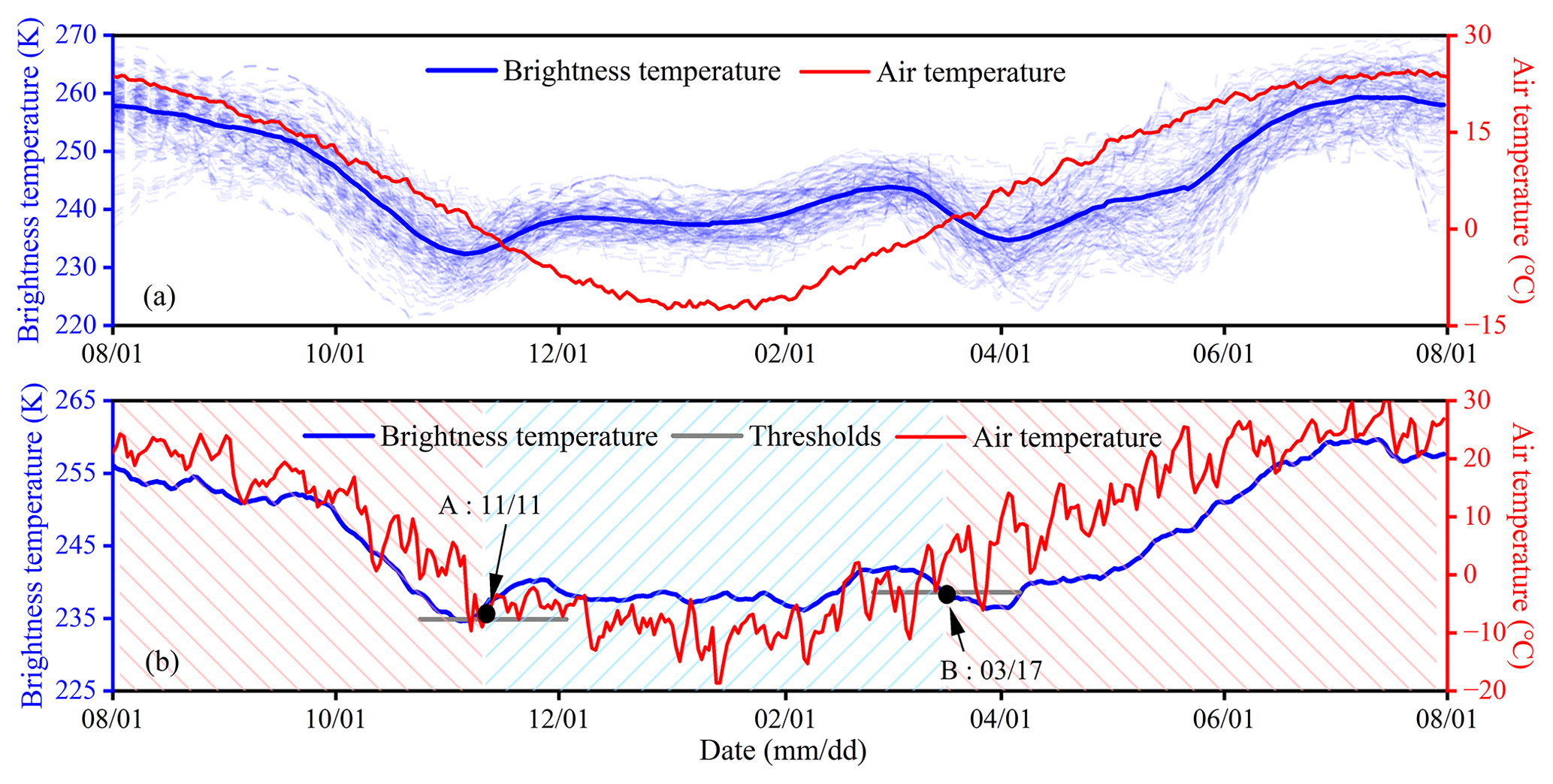
Figure 3 (a) Time series of brightness temperatures (dashed blue lines) for each hydrological year from 1979 to 2023. A hydrological year (HY) was defined from 1 August to 31 July of the following year for Lake Ulansu. (b) The brightness temperature (solid blue line) and air temperature (solid red line) for HY2001. The ice and water statuses were determined via the double-threshold moving t-test algorithm, where the red- and blue-shaded regions represent the water and ice states, respectively.

The DMTT originated from the moving t test (MTT), which was initially employed to identify abrupt meteorological change points in time series (Jiang and You, 1996; Shi and Zhu, 1996) and was later adapted by Du et al. (2017) to detect the abrupt change point (ACP) of T_b in passive microwave time series, enabling the discrimination of lake ice phenology. In this study, we enhanced the MTT to identify the ACP of the T_b series of complex mixed pixels in Lake Ulansu. Daily air temperature was also introduced to identify more suitable ACPs, facilitating the computation of the FUS and BUE dates. For the detailed steps and formulas of the MTT, refer to Du et al. (2017). Here, we specifically highlight the improvements of the DMTT:

• Step 1. In addition to adhering to the ACP criteria outlined by Du et al. (2017), we tailor the DMTT algorithm to detect ACPs by accounting for seasonal variations and specific thermal conditions. We conducted separate ACP detection for T_b from August to December and from January to July. To ensure the accuracy of the ACP in indicating freezing transitions, ACPs detected from August to December were validated only if they were accompanied by air temperatures below the freezing point. Similarly, for ACPs from January to July, a prerequisite condition of air temperatures above the freezing point was applied to confirm melting transitions. The purpose of these two enhancements was to accommodate the variations in mixed pixels during the transitions between water and ice.

• Step 2. After multiple ACPs are detected in Step 1, we calculate $\stackrel{\mathrm{‾}}{T_{\mathrm{b}\mathrm{1}}}$ and $\stackrel{\mathrm{‾}}{T_{\mathrm{b}\mathrm{2}}}$ for each ACP, which represent the mean T_b 20 d before and after the ACP, respectively. The freezing threshold was determined as the mean of the minimum $\stackrel{\mathrm{‾}}{T_{\mathrm{b}\mathrm{1}}}$ and its corresponding $\stackrel{\mathrm{‾}}{T_{\mathrm{b}\mathrm{2}}}$ within the same group, whereas the melting threshold was defined as the mean of the minimum $\stackrel{\mathrm{‾}}{T_{\mathrm{b}\mathrm{2}}}$ and its associated $\stackrel{\mathrm{‾}}{T_{\mathrm{b}\mathrm{1}}}$ within the same group. The DMTT algorithm calculates distinct thresholds for the FUS and BUE dates (solid gray lines in Fig. 3b), which makes it possible to handle various ice–water transition scenarios. This adaptability to different T_b series ensured the robustness of the algorithm (Appendix B).

• Step 3. We classified each T_b series via two thresholds to determine the ice and water pixel status. As demonstrated in Fig. 3b for a grid in Lake Ulansu in 2021, the interface between the red- and blue-shaded regions indicates the transitions between states, with points A and B marking the dates of these transitions in the T_b series. Given that five CETB grids (Fig. 1b) were selected within Lake Ulansu, the first date in the year when the status transitioned from water to ice was defined as the FUS date. Similarly, the first date when the transition occurred from ice to water was defined as the BUE date, with the ICD being the difference between these two dates. Based on this, we applied the DMTT algorithm to calculate thresholds and classify the CETB data, obtaining the ice phenology of Lake Ulansu from 1979 to 2023.

3.2.2 Estimation of ice phenology with the random forest model

For the period from 1941 to 1978, when satellite remote sensing data were unavailable, the random forest (RF) algorithm was employed to estimate the ice phenology of Lake Ulansu. The RF model is a powerful ensemble learning technique widely used for data modeling and prediction. Model accuracy can be improved by integrating the results of multiple decision trees (Breiman, 2001). Model robustness is particularly crucial when dealing with complex meteorological data for predicting ice phenology (Ruan et al., 2020). Previous research has highlighted the influence of short-term meteorological factors on the freezing and melting of shallow lakes (Blagrave and Sharma, 2023; Caldwell et al., 2020). Hence, we opted to employ a 3-month meteorological dataset to train the RF model, which was aligned with the characteristics of Lake Ulansu.

To train and validate the RF model, we randomly divided the dataset, which includes ERA5 meteorological factors and ice phenology derived from T_b data for the period from 1979 to 2023, into two subsets. A total of 70 % of the data were designated for training purposes, whereas the remaining 30 % were set aside for validation. Each subset was further segmented into two parts: the first part comprised the average air temperature, wind speed, solar radiation, and cumulative precipitation for September, October, and November, which were utilized in predicting the FUS dates. The second part mirrored the first in terms of meteorological variables but focused on the months of January, February, and March to predict the BUE dates. This organization resulted in each segment contributing 12 data points toward the prediction of each target variable, encapsulating the critical meteorological factors over the respective 3-month periods.

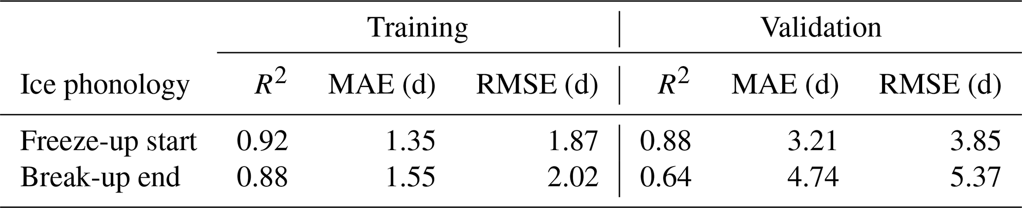
We employed the same hyperparameters (number of trees: 10, 20, 50, 100) as Anilkumar et al. (2023) did for glacier mass balance studies. Using grid search and evaluation, we considered the coefficient of determination (R²), mean absolute error (MAE), and root mean square error (RMSE) to select the hyperparameters. The optimal configuration was identified as 20 trees for both the FUS and BUE models (Appendix C), and 3-fold cross-validation was conducted on the training set. To further evaluate the efficacy of the RF model, we employed the R², MAE, and RMSE to assess its performance of the validation set. As shown in Table 1, the FUS model (R²=0.92) demonstrated superior performance compared to the BUE model (R²=0.88) within the training set. The MAEs for both models were less than 2 d. Furthermore, the results from the validation set deserve attention, with both models achieving R² values exceeding 0.6, underscoring the precision of the RF model in predicting the ice phenology of Lake Ulansu.

Table 1 Performance of the random forest model in predicting the freeze-up start date and the break-up end date. (R², MAE, and RMSE denote the coefficient of determination, mean absolute error, and root mean square error, respectively).

After the RF model was established and validated, we used ERA5 meteorological data from 1941 to 1978 as input features to obtain historical ice phenology. These data included average air temperature, wind speed, solar radiation, and cumulative precipitation for the months of September to November and January to March each year.

4 Results

4.1 Algorithm evaluation

The results of the DMTT algorithm were validated through a comparison with ice phenology data obtained from multisource optical satellite data from 2000 to 2023 (Sect. 3.1.2). Figure 4 reveals a remarkably high correlation for the FUS dates (r=0.92), with a minimal MAE of 2.00 d and an RMSE of 2.56 d. The correlation for the BUE date is slightly lower (r=0.87), with a somewhat greater MAE of 2.67 d and an RMSE of 3.25 d. However, the MAEs and RMSEs for the ICDs calculated based on the difference between the BUE and FUS dates remain within 5 d, indicating no systematic bias but random errors.

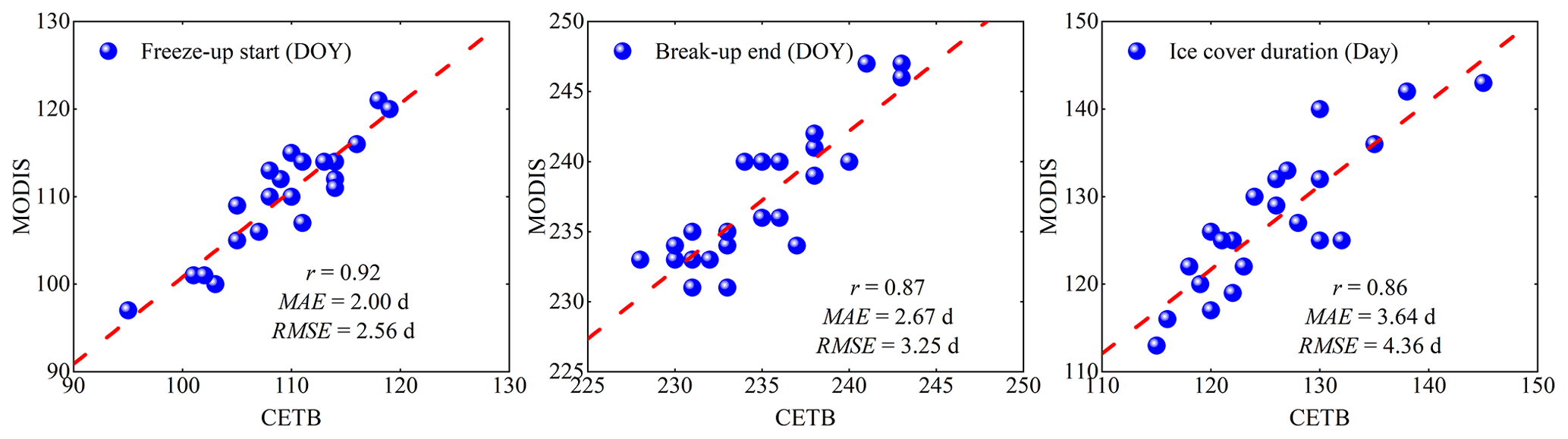
Figure 4 Comparison of the ice phenology extracted from the CETB data and from multisource optical satellites (2000–2023) for Lake Ulansu. The dashed red lines represent the linear regressions.

Figure 5 compares the ice phenology results calculated by the DMTT algorithm with those from the MTT algorithm and field observations. The MAEs between DMTT and MTT for the FUS, BUE, and ICD are less than 3 d. However, Du et al. (2017) reported that the MTT algorithm had significant limitations when it was applied to the ice phenology of Lake Ulansu between 2002 and 2015. Due to complex lake surface conditions, such as mixed pixels containing aquatic vegetation or land, approximately 49 % of the pixels were misclassified. As a result, the MTT algorithm could provide valid data for 5 to 8 years, which greatly reduced the continuity and accuracy of the ice phenology. In contrast, the new DMTT algorithm has been demonstrated to handle these complexities successfully, reducing misclassified states and substantially enhancing the accuracy of the dataset. Despite the scarcity of field observations, these data play a pivotal role in validating the precision of the DMTT algorithm (Fig. 5).

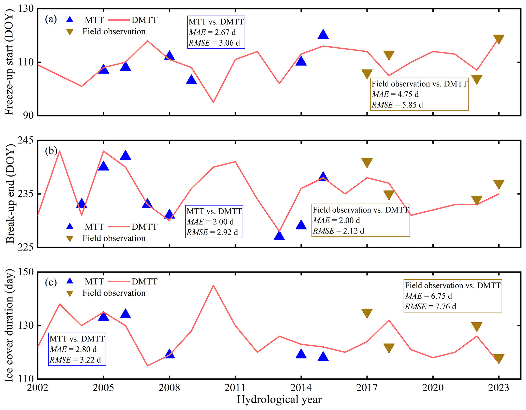
Figure 5 Comparison of the ice phenology for Lake Ulansu extracted via the DMTT algorithm (2002–2023) with that extracted via the MTT algorithm (2002–2015) and field observations (HY2017, HY2018, HY2022, and HY2023).

4.2 Ice phenology during 1941–2023

The ice phenology, including the FUS and BUE dates and the ICD of Lake Ulansu from 1941 to 2023, is shown in Fig. 6. To identify significant changes in the ice phenology trends, we calculated the 21-year moving averages for the FUS, BUE, and ICD (Appendix D). The ice phenology trends after 1982 were somewhat opposite to those before 1982, with this reversal being particularly pronounced in the ICD. To provide a detailed depiction of this reversal, we divided the whole period into two subperiods in the following analyses, and the corresponding statistical results are presented in Table 2.

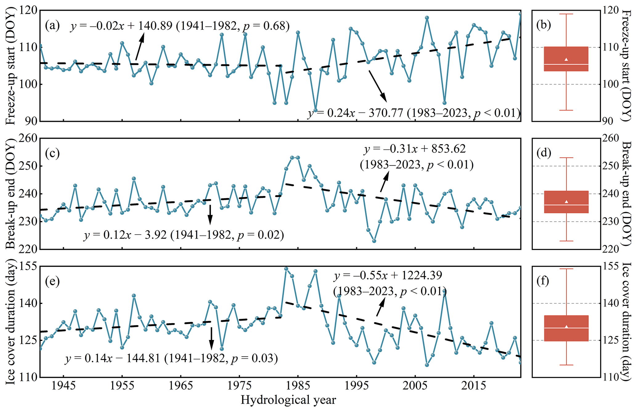
Figure 6 Ice phenology results for Lake Ulansu from 1941 to 2023. (a) Freeze-up start with trend lines. (b) Freeze-up start date distribution. (c) Break-up end with trend lines. (d) Break-up end date distribution. (e) Ice cover duration with trend lines. (f) Ice cover duration distribution.

Table 2 Average (Avg) and linear trend (Lt) of ice phenology in Lake Ulansu for various periods covering the years 1941 to 2023. Significance levels for trends are denoted by ^* (p<0.05) and ${}^{**}$ (p<0.01). DOY: day of year.

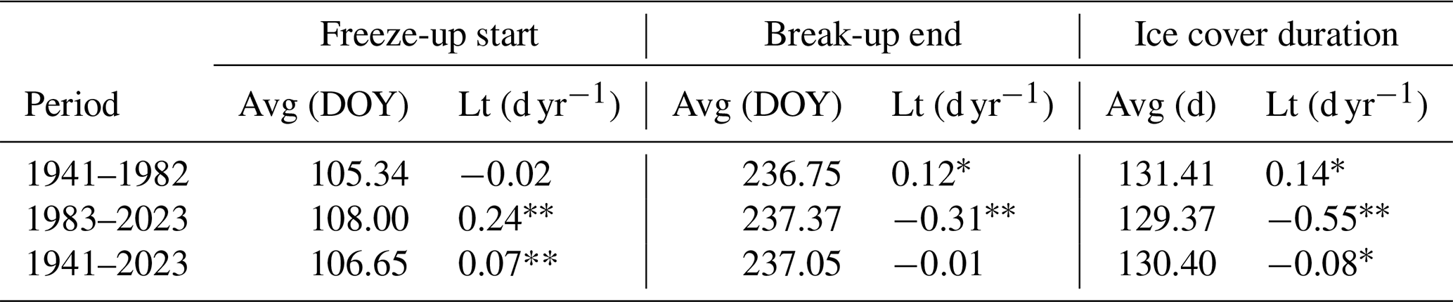
During the period from 1941 to 1982, the average date for FUS was approximately the 105th day (13 November), with an advance of 0.02 d yr⁻¹. The BUE date trend was more significant, with a delay of 0.12 d yr⁻¹, resulting in an average increase of 0.14 d yr⁻¹ in the ICD. Notably, the three ice phenology trends from 1983 to 2023 are highly significant (p<0.01). During this period, the FUS date exhibited a delay trend, advancing by an average of 0.24 d yr⁻¹, whereas the BUE date showed an early trend, advancing by an average of 0.31 d yr⁻¹. However, the ICD decreased by an average of 0.55 d yr⁻¹. These trends contrast with the ice phenology trends from 1941 to 1982 and are characterized by more pronounced trends.

Overall, from 1941 to 2023, the ice phenology in Lake Ulansu exhibited several notable features. The FUS occurred between the 93rd and 119th days, with an average date of approximately the 107th day (15 November), showing a slight delaying trend of 0.07 d yr⁻¹. The BUE ranged from the 223rd to the 253rd day, typically occurring around the 237th day (25 March), with an advancing trend of 0.01 d yr⁻¹. The ICD spans from 115 to 154 d, with an average of approximately 130 d, decreasing by 0.08 d yr⁻¹ over the study period.

4.3 Impact of meteorological factors on ice phenology

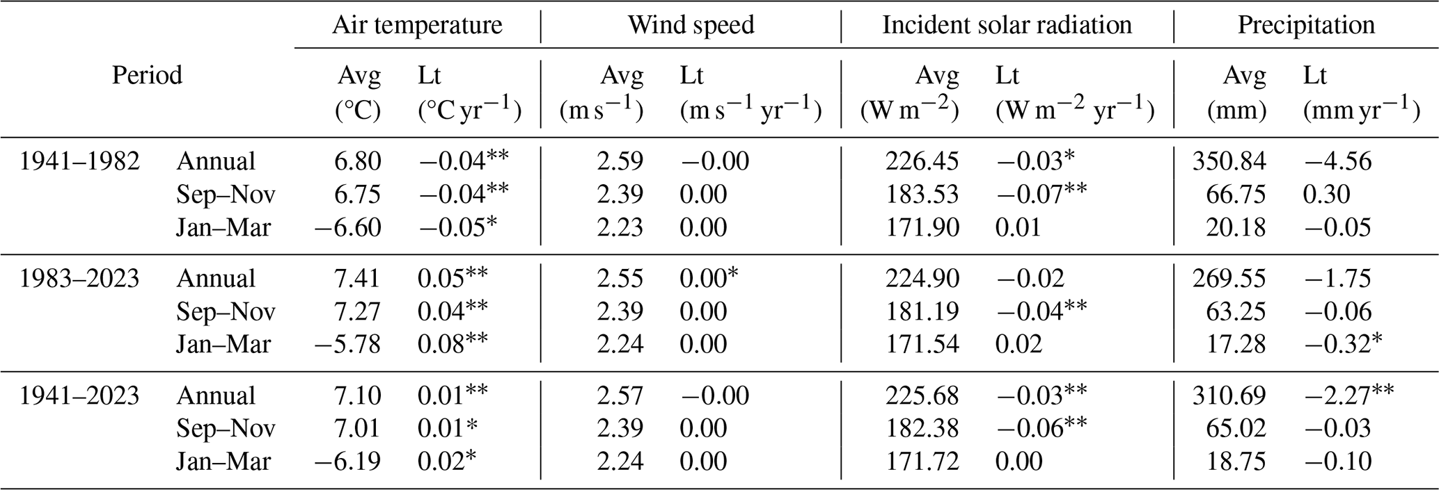
Ice phenology is determined primarily by local meteorological conditions (Bartosiewicz et al., 2021; L'Abée-Lund et al., 2021), and Table 3 summarizes the variations in the key meteorological factors influencing Lake Ulansu's ice phenology from 1941 to 2023. The changes in air temperature are clearly consistent with those in ice phenology, as shown in Fig. 6. From 1941–1982, the average air temperature decreased by 0.04 °C yr⁻¹ from September to November and accelerated to 0.05 °C yr⁻¹ from January to March. This cooling trend coincided with an advanced FUS date and a delayed BUE date, extending the ICD (Table 2). Conversely, from 1983 to 2023, both periods experienced increases in average air temperature at rates of 0.04 and 0.08 °C yr⁻¹, respectively. This warming trend was associated with a delayed FUS date and an advanced BUE date, indicating a decreased ICD. The observed air temperature fluctuations echo broader climate changes and show trends similar to those observed in other lakes (Magee et al., 2016; Newton and Mullan., 2021). Importantly, these shifts, which are particularly pronounced during the ice season, underscore the tight connection between ice phenology and regional climate dynamics (Marengo and Camargo, 2007).

However, variations in other meteorological factors are not as pronounced as those in air temperature. The wind speed remained relatively stable across these years (Table 3). The incident solar radiation decreased notably from September to November in accordance with the autumn–winter transition. Most of the precipitation occurred during the non-ice season. The months from September to November accounted for 18 % to 24 % of the annual precipitation, whereas the months from January to March contributed approximately 6 %, suggesting a minimal impact of snow cover formation on the ice surface due to its thinness.

To further understand the overarching influence of these meteorological factors, the previous RF model was also employed to rank the importance of each factor and determine their cumulative contributions to the FUS and BUE dates over specific periods (9–11 months and 1–3 months). As the predominant driver of changes in ice phenology, air temperature accounted for 56.5 % and 67.3 % of the variation in the FUS and BUE dates, respectively (Appendix E). This approach is straightforward because, among all meteorological factors, air temperature is the most important factor for controlling the heat balance at lake surfaces (Imrit and Sharma, 2021; Kropáček et al., 2013). In addition to air temperature, incident solar radiation contributed 20.1 % to the variation in the FUS dates and 15.0 % to the variation in the BUE dates. As seasons have transitioned, the decreasing intensity of solar radiation has reduced its heating effect on lake ice. The influence of precipitation was slightly more pronounced on the BUE date (14.7 %) than on the FUS date (12.3 %). Despite the limited precipitation in winter in Lake Ulansu, the snow cover significantly altered the heat budget of the lake ice. The high albedo of snow cover reflects a considerable amount of solar radiation, while its low thermal conductivity impedes the transfer of heat to the underlying ice (Cao et al., 2021). These combined effects slowed the ice-melting process, thereby delaying the onset of the BUE. The wind speed had a relatively high influence on the FUS (11.0 %), primarily by promoting water mixing and increasing heat exchange between the atmosphere and the water, thus affecting the formation of lake ice. For the BUE date, while the effect of wind speed was associated primarily with mechanical cracking of the ice cover, especially when it was thin, Lake Ulansu's relatively low wind speeds tempered this influence, resulting in a modest influence of only 3.1 % on the BUE date.

Table 3 Average (Avg) and linear trend (Lt) of meteorological factors in Lake Ulansu for various periods covering the years 1941 to 2023. Significance levels for trends are denoted by ^* (p<0.05) and ${}^{**}$ (p<0.01).

4.4 Monthly influence of meteorological factors on ice phenology

Although a holistic view of the contributions of meteorological factors to ice phenology is available in Appendix E, understanding that their influence is not equally important throughout the year is crucial. For example, air temperature, which is considered paramount (Bartosiewicz et al., 2021; Newton and Mullan, 2021), in particular influences ice cover formation during its initial weeks to months. Therefore, detailed analyses revealing the impact of monthly variations in meteorological factors on ice phenology are necessary, and the results are shown in Fig. 7.

Our analysis, depicted in Fig. 7a, shows that November's air temperature correlated most strongly with the FUS dates (r=0.53). This strong correlation can be attributed to the lake's shallow 1.6 m deep water, which allows for rapid responsiveness to cold air. As air temperatures decrease, the gradient between the lake and the atmosphere increases, leading to continuous heat release from the water to the atmosphere (Lazhu et al., 2021). This dynamic causes the surface water temperature to decrease swiftly, increasing the density of the upper water layer and triggering vertical convection. The resulting sinking of the upper water layer expedites the cooling of the entire waterbody. This effect of air temperature is not confined to the FUS date; it extends to the BUE date (Fig. 7b), with the strongest correlation coefficients found for February ($r=-\mathrm{0.49}$) and March ($r=-\mathrm{0.70}$). The cumulative thickness of the ice cover during its formation period impacts the timing of the melting period. Therefore, the air temperature from November to March had some impact on the BUE date, with r>0.3.

Surprisingly, the correlation coefficient for solar radiation was notably low (Fig. 7a), and in November, it exhibited a negative correlation with the FUS date ($r=-\mathrm{0.37}$). This trend is like the findings of Caldwell et al. (2020). For Lake Ulansu, the correlation may be due to the high attenuation coefficient caused by the presence of numerous suspended particles and algae, which are common in eutrophic lakes (Yang et al., 2020b). These particles and algae absorb and scatter solar radiation, especially blue light (450–495 nm), reducing the penetration depth of light in water (Lin et al., 2024). As a result, the heating effect of solar radiation is confined primarily to the surface layers, leading to a diminished overall heating effect on the water. Moreover, the incident solar radiation exhibited a decreasing trend, averaging between 119 and 125 W m⁻² in November. This not only limited the heating effect on the water but also suggested that the narrow range of variation might not capture the intricacies of its actual impact. Nonetheless, in January, solar radiation became more influential ($r=-\mathrm{0.33}$). Solar radiation heats the waterbody, increasing the ice–water heat flux and promoting ice cover melting.

Wind plays a dual role in this process. While it can accelerate water mixing, promoting early FUS, it can also disrupt fragile ice, delaying the formation of stable ice cover (Fig. 7a). At Lake Ulansu, where the wind speed generally ranges from 1 to 4 m s⁻¹, its influence on the FUS date was somewhat muted, as indicated by an r of −0.07 in November. Similarly, the effect of wind on the ice-melting phase is marginal (Fig. 7b). Primarily impacting the ice surface, subdued wind speeds at the lake contributed to a decrease in turbulent heat exchange and a consequent reduction in ice sublimation.

The role of precipitation is complex. When it manifested as rain over the lake in October, it cooled the water, narrowing the temperature gap between the lake and the atmosphere ($r=-\mathrm{0.13}$). Conversely, when it fell as snow in November, its low thermal conductivity obstructed heat exchange between the lake and the atmosphere, hampering the formation of a stable ice cover (r=0.27). If there is a considerable amount of snow cover, the influence of air temperature and solar radiation on the ice cover and the underlying water can be mitigated, but Lake Ulansu experiences limited snowfall, resulting in a minimal impact on the BUE date (Fig. 7b).

Since the ICD is the difference between the BUE date and the FUS date, the meteorological factors highly correlated with the ICD were essentially the same for both the FUS date and the BUE date (Fig. 7c). Air temperature remains the primary influencing factor, with the correlation coefficient of solar radiation in January also being relatively high.

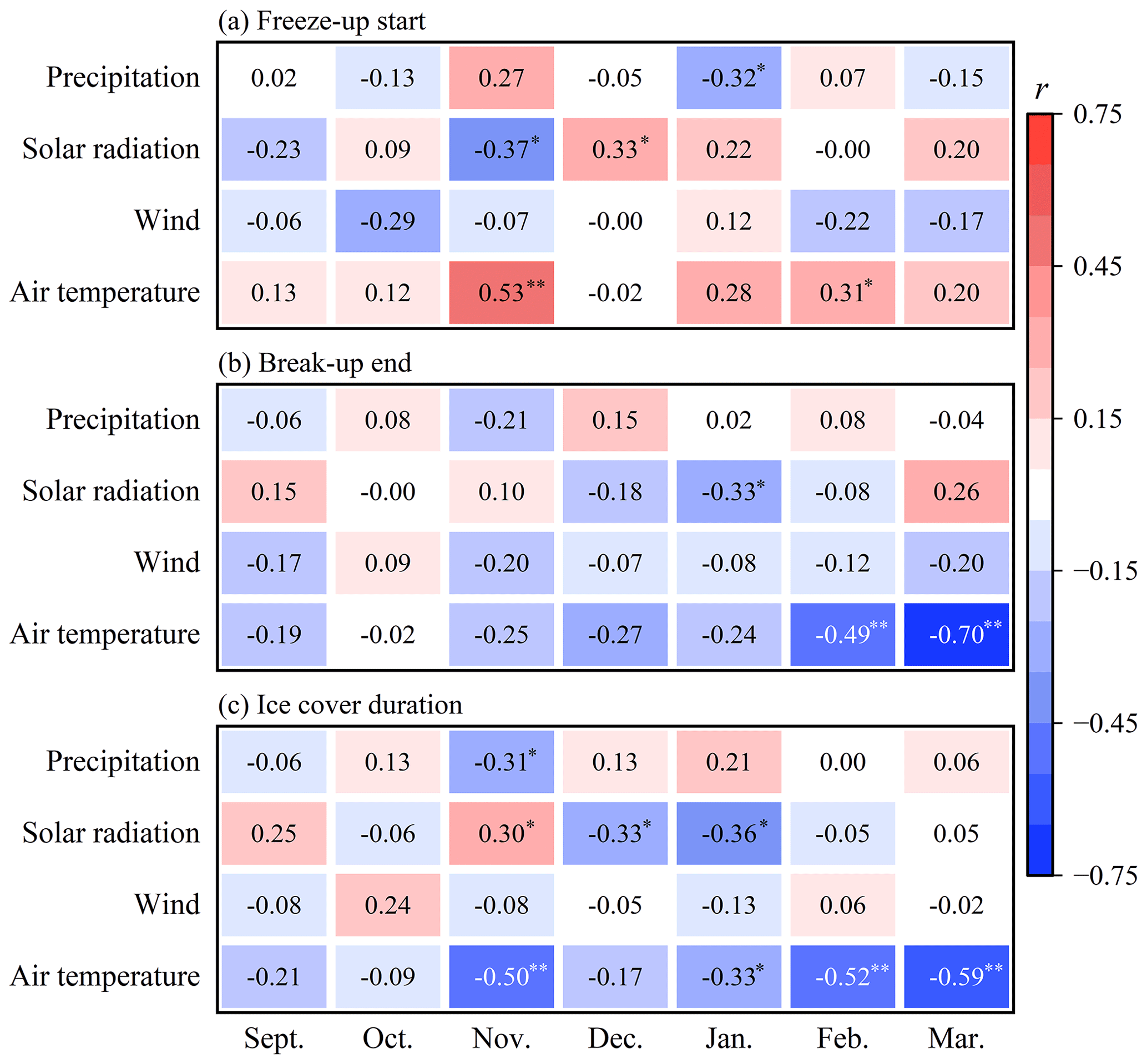
Figure 7 Correlation coefficients between meteorological factors and ice phenology in different months. Significance levels for correlation coefficients are denoted by ^* (p<0.05) and ${}^{**}$ (p<0.01).

5 Discussion

The novel DMTT algorithm developed in this study has proven essential for accurately discerning ice and water states in a lake with mixed-pixel challenges. In this section, we discuss the uncertainties associated with methodologies, compare our findings with those of other studies, and elaborate on the implications of the results for understanding the impacts of climate change on lake ice phenology.

5.1 Uncertainty analysis

Owing to the specific characteristics of Lake Ulansu, the uncertainties in ice phenology reconstruction are attributed mainly to the spatiotemporal-resolution constraints of the CETB data and the methodological limitations associated with the DMTT algorithm used in the study.

First, the CETB T_b data had a high spatial resolution of 3.125 km. Owing to the complex geometry of the shoreline and rich aquatic vegetation of reeds in Lake Ulansu, five CETB grids with water coverage exceeding 0.70 were selected (Fig. 1b). The criteria for selecting these pixels were twofold: first, to ensure the inclusion of extensive water surfaces, thereby minimizing the influence of land surface T_b, and, second, to locate the pixels predominantly in the central area of the lake where the water depth is more consistent, thus reducing the effects of uneven ice formation due to depth variation. Considering the overall shallow depth of the lake, we contend that the potential error caused by our grid selection is minimal when assessing the ice phenology of Lake Ulansu. Furthermore, despite the 1 d temporal resolution of the CETB data, periodic gaps in the T_b data may occur due to orbital issues. This problem is particularly pronounced in the SMMR sensor and could lead to a maximum error of approximately 5 d in the ice phenology results for the years 1979–1987 (Cai et al., 2022). However, T_b data from SSM/I and SSMIS are more complete, resulting in more accurate ice phenology data from these sensors (Fig. 4).

Second, the DMTT algorithm applies a smoothing technique to calculate the daily values of T_b as the average of the preceding 10 d and the following 10 d, following Du et al. (2017). The purpose of this step was to eliminate the influence of short-term fluctuations on the T_b data but at the cost of losing some T_b information. Furthermore, the DMTT algorithm uses CETB data at 37.5 GHz. However, Kang et al. (2012) reported that 18.7 GHz is more suitable for calculating the BUE date when analyzing phenological data for Great Bear Lake and Great Slave Lake because of large changes in T_b during the transition of ice into water, facilitating the detection of ACPs. This discrepancy may explain the slightly inferior BUE results in this study (Fig. 4). However, the coarse spatial resolution of 18.7 GHz in the CETB data is unsuitable for determining the shape of the shoreline of Lake Ulansu. Considering this, our study employed two thresholds to separately calculate FUS and BUE dates, obtaining thresholds better suited for the transition between ice and water states and thereby enhancing the accuracy of ice phenology results.

5.2 Comparison with other lakes

Lake Ulansu is characterized by its shallow depth and abundant aquatic vegetation, which is much different from most previous results on large lakes at similar latitudes and boreal lakes with heavy snowfall. Therefore, a comparison between these lakes and the general trends across lakes in the Northern Hemisphere is interesting.

First, unlike previous studies on lake ice phenology using passive microwave data that focused primarily on large lakes due to algorithm limitations, this study develops the DMTT algorithm, revealing distinct ice phenology for the shallow, vegetated Lake Ulansu. A direct comparison with Qinghai Lake is straightforward because they are at similar latitudes, but the latter is a massive saline lake on the Tibetan Plateau, covering an area of more than 4000 km², with a much larger water volume than Lake Ulansu. Cai et al. (2017) used T_b data to calculate the ice phenology of Qinghai Lake from 1979 to 2016. They reported that the FUS date delay and BUE date advancement were 0.16 d yr⁻¹ and 0.37 d yr⁻¹, respectively, which are weaker and stronger than those observed for Lake Ulansu. During the freezing process, more heat must be released to cool the lake water than in a shallow lake. This makes it relatively less sensitive to air temperature fluctuations in Qinghai Lake than shallow lakes are, hence resulting in a weak trend for the FUS dates. At altitudes greater than 3000 m, ice melt in Qinghai Lake is markedly influenced by its exposure to intense solar radiation, leading to a more pronounced BUE trend (Kirillin et al., 2021). Additionally, factors such as sublimation due to strong winds also significantly impact BUE dates, with studies such as Huang et al. (2019) showing that sublimation accounts for up to 40 % of the maximum ice thickness loss in the region. Various factors contribute to the pronounced BUE trends in lakes on the Tibetan Plateau. In contrast, long-term studies of Lake Ulansu indicate a stronger trend for FUS than for BUE (Table 2), with air temperature exerting an influence of over 50 % on both the FUS and BUE dates.

Second, the impacts of precipitation, particularly snow, on ice phenology strongly differ between Lake Ulansu and northern European lakes. Research on Estonian lakes by Nõges and Nõges (2013) illustrates that despite rising air and lake surface temperatures from 1961 to 2004, the BUE date displayed only minimal changes. This anomaly is attributed to the insulating properties of snow, which moderate the thermal response of lakes to climatic warming (Cheng et al., 2020). Thus, the insulating effect of heavy snowfall was substantial enough to offset the rising air temperature's potential to advance the BUE date. In contrast, Lake Ulansu's region experiences markedly less winter precipitation (Table 3), resulting in minimal snow cover. The sparse snowfall, coupled with wind activity that disrupts snow accumulation, diminishes any insulative buffer on the ice surface, allowing for air temperature to exert a more direct influence on the BUE date than Estonian lakes do. Furthermore, in northern European lakes, minimal solar radiation during winter is largely reflected by the high albedo (>0.7) of heavy snow cover (Gebre et al., 2014), which, together with the high albedo (>0.5) of snow ice (Leppäranta et al., 2010), significantly reduces the influence of solar radiation on ice-melting processes. Conversely, in Lake Ulansu, where the surface albedo is much lower (<0.3) (Cao et al., 2021), the influence of solar radiation on the melting process is much greater. This makes the BUE responsive to solar radiation. In regions such as Lake Ulansu, where snow cover does not significantly mitigate the effects of air temperature and solar radiation, understanding the direct impacts on ice phenology provides critical insights into how similar ecosystems might respond under scenarios of diminishing snowfall due to climate change.

Finally, an analysis by Newton and Mullan (2021) on ice phenology across 678 waterbodies in the Northern Hemisphere from 1931 to 2005 highlighted a modest overall increase in the ICD of 0.06 d yr⁻¹. In contrast, Lake Ulansu exhibited a more pronounced trend in the ICD, underscoring its heightened sensitivity to climatic variations due to its shallow depth and unique regional climate conditions. This significant divergence from broader hemispheric trends demonstrates the critical need to include diverse lake types, such as shallow lakes and small and medium-sized lakes, in climatic impact studies. Detailed insights into Lake Ulansu's ice phenology reveal how subtle fluctuations in air temperature can have amplified effects on shallow lakes, making them essential indicators of ecological responses to global climate change.

6 Conclusion

To our knowledge, we reconstructed the ice phenology of Lake Ulansu from 1941 to 2023, the longest ice phenology data for a large, shallow, and aquatic-plant-dominated lake in northwestern China. A new double-threshold moving t-test (DMTT) algorithm was developed to distinguish water and ice from lake surfaces via 37 GHz H-polarization T_b data with a resolution of 3.125 km from the CETB dataset. The DMTT has integrated daily air temperature, which allows it to accurately detect abrupt change points (ACPs) and thus calculate distinct thresholds for transitions between water and ice. This enhanced functionality allowed us to effectively differentiate mixed pixels among complex shorelines and rich aquatic vegetation, resulting in accurate ice phenology data from 1979 to 2023. Together with the corresponding meteorological data, these data further served as training data for the RF model, and the ice phenology of Lake Ulansu from 1941 to 1978 was successfully reconstructed.

Over the 83 years from 1941 to 2023, Lake Ulansu presented an average FUS date of 15 ± 5 November and an average BUE date of 25 ± 6 March, with an average ICD of 130 ± 8 d. The trends in the FUS, BUE, and ICD dates were 0.07, −0.01, and −0.08 d yr⁻¹, respectively. Notably, we did not find significant trend changes in the delayed FUS and advanced BUE dates. This phenomenon can be attributed primarily to significant air temperature fluctuations in the 1980s, characterized by a cooling trend before the 1980s and a warming trend thereafter. Over the last 4 decades, considerable contraction in the ice cover span has occurred, with the ICD shortening by an average of 22 d, markedly contrasting with the more gradual trends observed in the ICD across other lakes in the Northern Hemisphere (Newton and Mullan, 2021). The predominant role of air temperature in ice phenology has been confirmed, showing that it contributes 56.5 % of the variation in the FUS date and 67.3 % of the variation in the BUE date. Seasonal transitions further underscore the role of air temperature, particularly in November, where it strongly correlates with the FUS date (r=0.53) and extends into early spring, influencing the BUE date ($r=-\mathrm{0.50}$). The high eutrophication level in Lake Ulansu attenuates the capacity of solar radiation to heat the waters, with the most substantial influence observed during the ice-melting process in January, as evidenced by a correlation coefficient of $r=-\mathrm{0.36}$. Wind speed, while contributing to water mixing and early ice formation, has a limited effect on the FUS date and an even lesser impact on the BUE date due to the lake's generally low wind conditions. The role of precipitation is complex, with rain cooling the water and snow impeding heat exchange because of its low thermal conductivity, yet both have a minimal overall impact on the BUE date considering the lake's limited snowfall. Overall, wind speed, precipitation, and solar radiation collectively accounted for 43.5 % of the influence on the FUS date and 32.7 % on the BUE date, highlighting the multifaceted yet secondary roles of these factors in shaping the ice phenology of Lake Ulansu compared with the predominant role of air temperature.

This study introduced the new DMTT algorithm, which significantly enhances the capability for ice phenology research in lakes with complex shorelines and abundant vegetation. Given the presence of W-shaped T_b series lakes across the Northern Hemisphere (Appendix F), plans include extending this algorithm's application to a broader range of small and medium-sized lakes globally. Additionally, the data gaps in early satellite records, particularly those of Nimbus 7, warrant further investigation to achieve a more comprehensive historical perspective. Addressing these gaps is crucial for enhancing the accuracy of long-term ice phenology reconstructions. We also expect future research to delve into the composition, chemical properties, and microstructure of lake ice through numerical simulations, thereby opening new possibilities for remote sensing applications across various lake types.

Appendix A: ERA5 meteorological data evaluation

The daily average air temperature, wind speed, and incident solar radiation were calculated and compared with available field observations from 2016 to 2018 and from 2022 to 2023 (Cao et al., 2021; Lu et al., 2020). As shown in Fig. A1a, there was significant agreement between the ERA5 air temperature data and the field observations, with an r of 0.99. The MAE was 0.95 °C, and the RMSE was 1.17 °C. Further error reduction was achieved by applying a regression equation to adjust the air temperature. This high accuracy of air temperature ensures the precision of subsequent ice phenology calculations based on CETB data. Although the reanalysis gridded data may struggle to capture near-surface true wind speeds, the ERA5 wind speed data exhibited greater consistency in inland areas than other reanalysis datasets did (Ramon et al., 2019). A correlation coefficient of r=0.81 was achieved by comparison with field observations, as shown in Fig. A1b, and the error for the wind speed data over Lake Ulansu further decreased to an MAE of 0.48 m s⁻¹ and an RMSE of 0.61 m s⁻¹ after linear regression was applied. Overall, the incident solar radiation data from this dataset were slightly lower than those from the field observations (Fig. A1c), but the corrected daily averages were within acceptable limits, with an MAE of 18.04 W m⁻² and an RMSE of 22.35 W m⁻². Previous studies have indicated that the use of ERA5 precipitation data has significant advantages and that these data are widely used in various regions (Bandhauer et al., 2021; Yuan et al., 2021). In this study, cumulative precipitation was calculated for ice phenology trend analyses for Lake Ulansu. Its validity is not presented here because of the absence of in situ precipitation observations in this region, with only limited snowfall or thin snow cover (<4 cm) occurring in the winter (Lu et al., 2020).

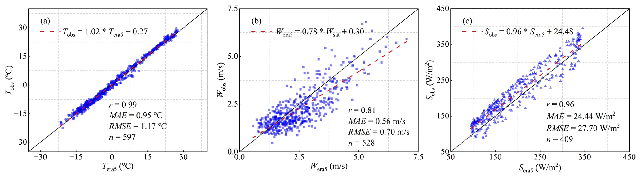
Figure A1 Comparison between ERA5 and observed daily average (a) air temperature (T_era5, T_obs), (b) wind speed (W_era5, W_obs), and (c) incident solar radiation (S_era5, S_obs) meteorological data for Lake Ulansu. r, MAE, RMSE, and n denote the correlation coefficient, mean absolute error, root mean square error, and sample size, respectively.

Appendix B: Adaptability of the DMTT algorithm in the brightness temperature series

The DMTT algorithm shows strong adaptability in identifying the T_b series from mixed pixels. Although these series maintain a W shape overall, there are differences in the specific T_b during the freezing and melting stages. Figure B1a shows smaller changes in brightness temperature between these two stages, and Fig. B1b shows a lower T_b valley during melting than during freezing. Such sensitivity to nuanced changes underscores the substantial advantage of the DMTT algorithm in enhancing the precision and continuity of long-term ice phenology data, especially in environments with complex shorelines and extensive aquatic vegetation.

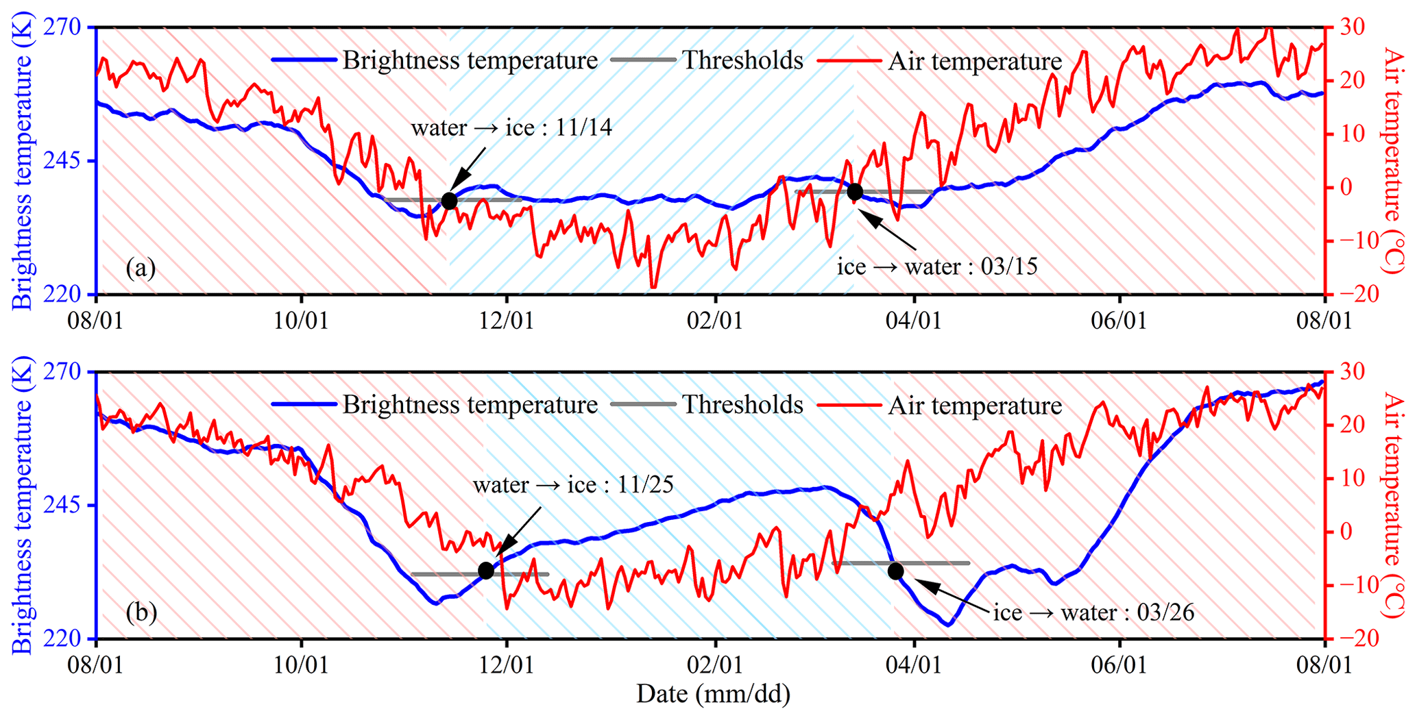
Figure B1 Brightness temperature (solid blue line) and air temperature (solid red line). The ice–water status was determined via the double-threshold moving t-test algorithm, where the red- and blue-shaded regions represent the water and ice states, respectively. (a) HY2001 and (b) HY2015.

Appendix C: Optimal number of trees for the random forest model of ice phenology

In the process of hyperparameter optimization for our random forest model, we carefully considered the balance between model complexity and predictive accuracy. A greater number of trees, such as 100, might yield a lower MAE for the training set, which is also associated with a greater risk of overfitting. Overfitting occurs when a model learns the training data too well, including noise and outliers, which results in decreased performance for unseen data, as evidenced by a larger MAE for the validation set (Table C1).

By selecting 20 trees, we strike an optimal balance where the model complexity is sufficient to capture the underlying patterns in the data without being overly sensitive to the noise in the training data. We observed that increasing the number of trees from 20 to 100 did not significantly improve the R² for the training set. Moreover, for the FUS model, there was a notable decrease in R² for the validation set when 50 or 100 trees were used compared with 20 trees. This indicates that the additional complexity introduced by more trees may lead to overfitting, which harms the model's predictive performance for new data. Moreover, the performance of the validation set for models with 20 trees suggests robust generalization without significant overfitting, as indicated by consistent R² values and acceptable MAE and RMSE values. Therefore, considering the potential for overfitting, the computational efficiency, and the model's generalization performance, we concluded that a configuration of 20 trees is the most appropriate for our study.

Table C1 Performance of freeze-up start date and break-up end date predictions for training and validation sets with varying numbers of trees in a random forest model.

Appendix D: The 21-year moving averages of ice phenology

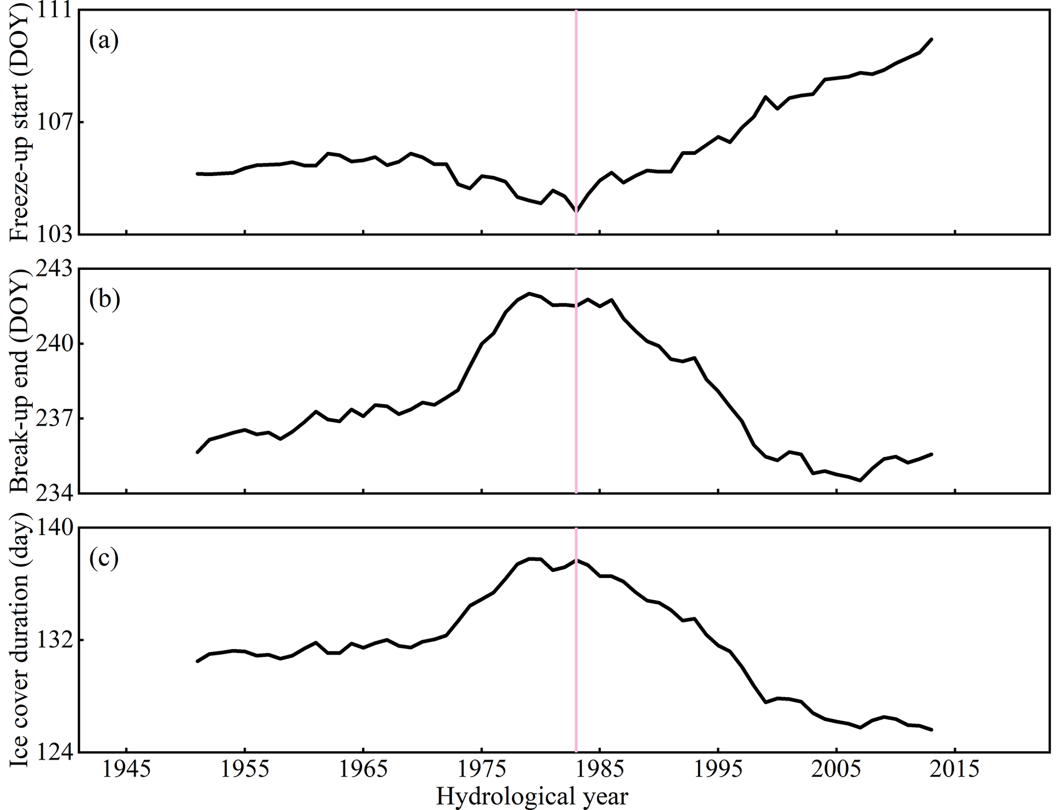
Figure D1 The 21-year moving averages of ice phenology for Lake Ulansu. (a) Freeze-up start. (b) Break-up end. (c) Ice cover duration. The vertical pink line indicates HY1983.

Appendix E: Contributions of meteorological factors to ice phenology

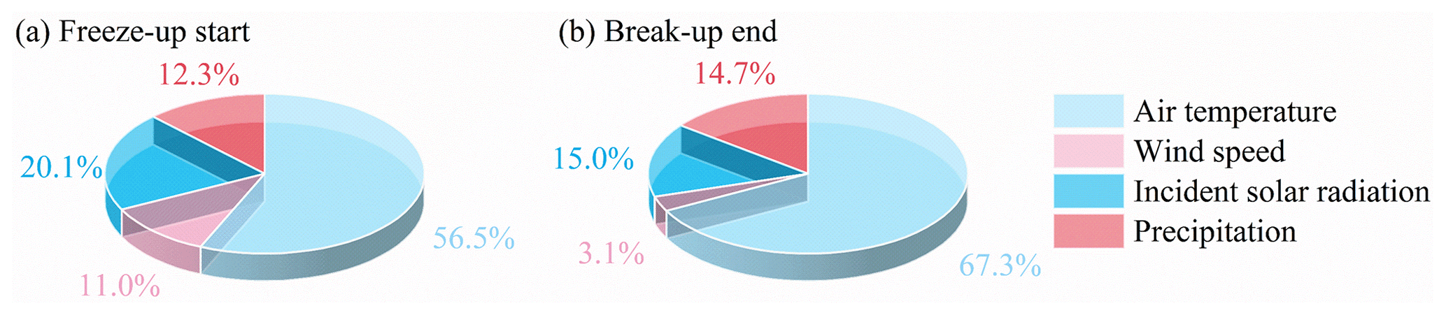
Figure E1 Contributions of meteorological factors to Lake Ulansu's freeze-up start and break-up end dates.

Appendix F: W-shaped brightness temperature series for diverse lakes across the Northern Hemisphere

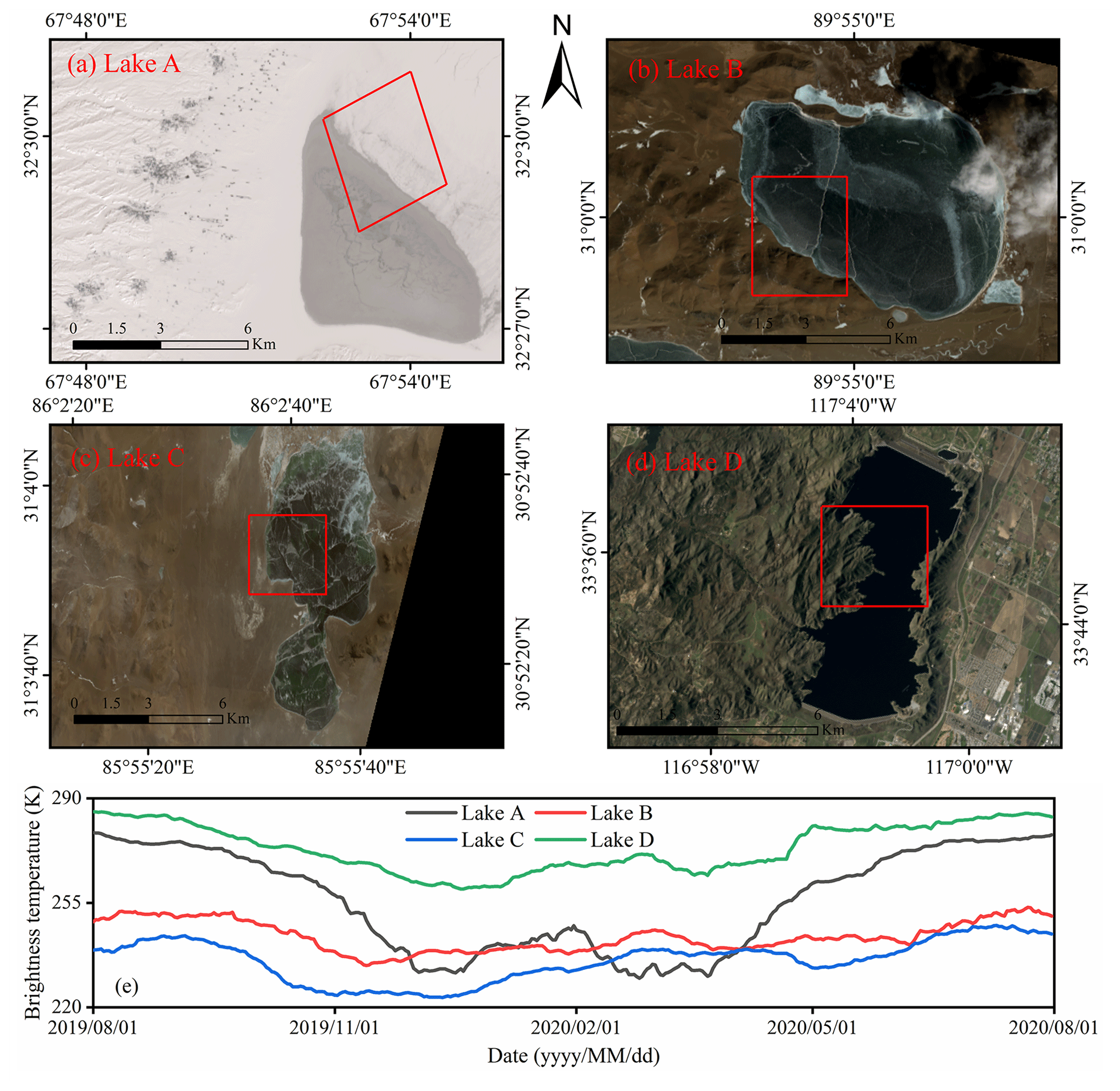
Figure F1 (a–d) Landsat 8 images of Lake A, Lake B, Lake C, and Lake D. Red rectangles indicate where mixed brightness temperature pixels were analyzed. (e) Brightness temperature time series from 1 August 2019 to 1 August 2020, for each lake.