A minimal machine-learning glacier mass balance model

Glacier retreat presents significant environmental and social challenges. Understanding the local impacts of climatic drivers on glacier evolution is crucial, with mass balance being a central concept. This study introduces miniML-MB, a new minimal machine-learning model designed to estimate annual point surface mass balance (PMB) for very small datasets. Based on an eXtreme Gradient Boosting (XGBoost) architecture, miniML-MB is applied to model PMB at individual sites in the Swiss Alps, emphasising the need for an appropriate training framework and dimensionality reduction techniques. A substantial added value of miniML-MB is its data-driven identification of key climatic drivers of local mass balance. The best PMB prediction performance was achieved with two predictors: mean air temperature (May–August) and total precipitation (October–February). miniML-MB models PMB accurately from 1961 to 2021, with a mean absolute error (MAE) of 0.417 m w.e. across all sites. Notably, miniML-MB demonstrates similar and, in most cases, superior predictive capabilities compared to a simple positive degree-day (PDD) model (MAE of 0.541 m w.e.). Compared to the PDD model, miniML-MB is less effective at reproducing extreme mass balance values (e.g. 2022) that fall outside its training range. As such, miniML-MB shows promise as a gap-filling tool for sites with incomplete PMB measurements as long as the missing year's climate conditions are within the training range. This study underscores potential means for further refinement and broader applications of data-driven approaches in glaciology.

1 Introduction

Glaciers in the European Alps are losing mass and retreating, a phenomenon that has been accelerating since the 1980s because of human activity (Zemp et al., 2008; Marzeion et al., 2014) and that is projected to continue in the future (e.g. Rounce et al., 2023). The environmental and societal consequences of this decline are substantial (IPCC, 2023), underscoring the need for accurate representations of glacier evolution through measurements and models.

A central concept for describing glacier evolution is mass balance (MB), which quantifies the change in a glacier's mass over time (Cogley et al., 2011). In the European Alps, with typically very limited frontal, basal, and internal MB processes, the total glacier MB is driven by the surface mass balance (SMB). SMB represents the net balance between surface accumulation (through solid precipitation, refreezing, wind-blown snow, and avalanches) and surface ablation (mainly through surface melt and sublimation) (Benn and Evans, 2014). In this work, we focus on point surface mass balance (PMB), which is determined by local ablation and accumulation processes and thus provides a direct climatic signal at a specific point on a glacier. PMB is essential for improving our knowledge of the local impact of climatic drivers of glacier change through accumulation and melting (Vincent et al., 2004; Huss et al., 2009; Vincent et al., 2017). Furthermore, PMB can also be used to calibrate and/or evaluate numerical models, which, in turn, can be used to simulate glacier evolution.

PMB can be measured through direct observations using labour-intensive field measurements with stakes and snow pits (Blake, 1993; Adams, 2011; Huss et al., 2015). In addition, PMB can be calculated with empirical or physically based models (e.g. Kuhn et al., 1999; Huss et al., 2008), but the necessary variables for complex numerical models, such as energy balance models, are generally unavailable, e.g. measurements of radiation and turbulent fluxes. New studies also propose techniques to retrieve PMB from elevation change and the inversions of ice thickness and velocity, but these PMB estimates carry considerable uncertainties (e.g. Van Tricht et al., 2021; Miles et al., 2021; Vincent et al., 2021; Cook et al., 2023b).

Recent studies have explored novel statistical methods using machine learning (ML) to model glacier evolution components, contrasting with conventional numerical approaches. For example, recent data-driven approaches have modelled glacier ice dynamics, a key component alongside MB for projecting glacier evolution (e.g. Jouvet et al., 2022; Bolibar et al., 2023; Jouvet, 2023; Jouvet and Cordonnier, 2023; Cook et al., 2023a). For MB, Bolibar et al. (2020, 2022) proposed an ML model of 21st-century glacier-wide SMB coupled to a glacier evolution module to predict glacier changes in the French Alps. However, this data-driven MB model did not contain information on the distribution of MB within a glacier (i.e. no local PMB information). A recent study by Anilkumar et al. (2023) explored the simulation of PMB based on World Glacier Monitoring Service data over the European Alps (WGMS, 2023). They assessed various ML architectures trained on an ensemble of glacier sites, focusing on the generalisability and transferability of the models across different sites. The study also investigated the impact of dataset size on model performance, though their smallest dataset (around 900 points) is relatively large in the context of PMB records. While they demonstrated the ability of tree-based models to identify relevant climatic drivers of MB, they did not investigate the MB drivers at specific sites.

This study introduces miniML-MB, a new minimal ML model designed to simulate annual PMB at individual glacier sites using meteorological variables (air temperature and total precipitation). Based on eXtreme Gradient Boosting (XGBoost) (Chen and Guestrin, 2016), miniML-MB is trained and evaluated separately at each site to account for site-specific PMB variability. Our model thus predicts PMB for a specific year based on measurements taken from the same site in other years. In this particular setup, input data are scarce, which is common in glaciology but challenging for data-driven ML applications. Here, we tackle this challenge by relying on dimensionality reduction techniques to reduce the input space in miniML-MB.

We rely on data collected at 28 individual MB measurement sites across the Swiss Alps (Fig. 1). Switzerland stands out for its extensive long-term glacier measurements compiled within the Glacier Monitoring in Switzerland (GLAMOS) programme, dating back to the early 20th century, notably for glaciers like Clariden and Silvretta (Huss et al., 2021).

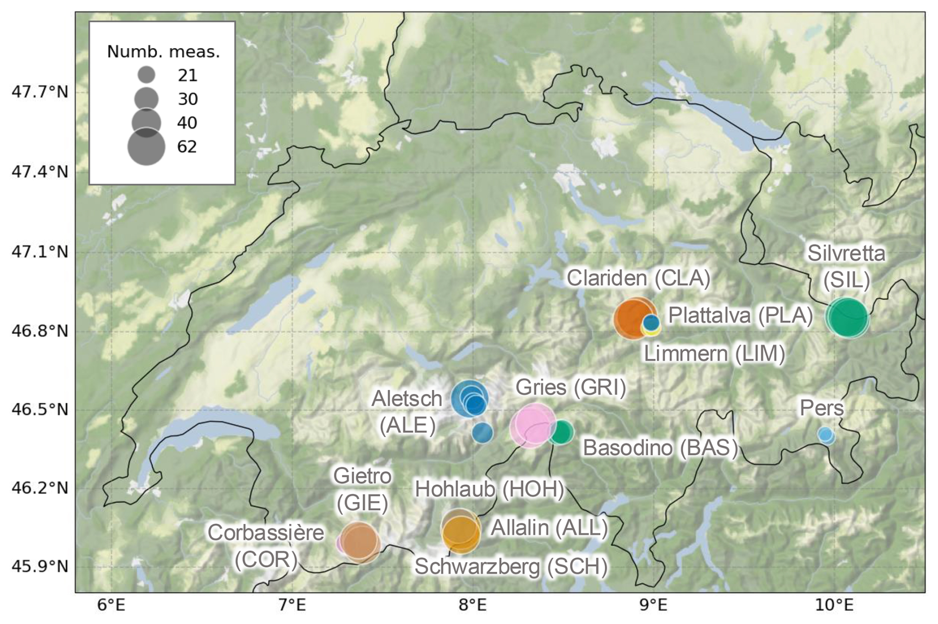
Figure 1 Overview of sites (individual mass balance stakes) with annual point surface mass balance measurements in the Glacier Monitoring in Switzerland (GLAMOS) network: 28 sites on 13 glaciers from 1961 to 2023. Each site is represented by a circle, coloured according to the glacier it belongs to (annotated in grey). The circle size represents the total number of years with measurements (ranging from 21 to 62). The background terrain map represents hill shading and natural vegetation colours by Stamen Design (2024).

We intentionally chose to model individual sites, thereby optimising the model in relation to each site's unique characteristics. Compared to modelling of multiple sites at once (e.g. Bolibar et al., 2020, 2022; Anilkumar et al., 2023), our approach allows the following:

1. Capturing climatic drivers at local scales. To determine the optimal dimensionality reduction approach for miniML-MB, we use feature-engineering techniques and estimate feature importance, allowing us to quantify the significance of individual climate features. This methodology offers data-driven insights into the meteorological variables that drive local PMB, e.g. highlighting which months' temperature and precipitation drive the MB variability.

2. Tailoring ML models to small glaciological datasets. Switzerland's abundant MB measurements offer an ideal platform for studying local data-driven PMB simulations at various sites. However, a key strength of our approach is that limited data are needed to train the model at each site, making it suitable for other regions with scarcer data. For example, remote areas with restricted field access, such as High Mountain Asia (Azam et al., 2018; Wester al., 2019) or the Andes (Mernild et al., 2015), have fewer individual glacier sites, hindering generalisation for a model trained on multiple sites. Understanding how to tailor ML models to fit very small datasets is crucial for effective local-scale modelling of these sites.

Section 3 provides an overview of the study site and the climate input data of the ML model, outlines the architecture, and introduces the training and evaluation frameworks. This study's core analysis focuses on PMB measurements up to 2021, initially excluding the prediction of the extreme MB years of 2022 and 2023 (SCNAT, 2023; Cremona et al., 2023; Voordendag et al., 2023). Section 4 describes the implementation of the positive degree-day (PDD) model used as a baseline for our ML model. In Sect. 5.1–5.3, we first compare different dimensionality reduction frameworks of miniML-MB before comparing the model's performance with that of the PDD baseline. Section 5.4 includes a separate analysis of the extreme years of 2022 and 2023, allowing us to test the model's predictive capability in such circumstances. Section 5.5 shows predictions made by miniML-MB when used as a gap-filling tool. Section 5.6 analyses the drivers of PMB in miniML-MB. Sections 6 and 7 examine the outcomes of these analyses and offer insights into both the broader applicability of miniML-MB and the future use of ML for predicting MB at various spatial and temporal scales.

2 Study site and data

2.1 Meteorological data

As predictors for our data-driven PMB model (see Sect. 3), we use two monthly meteorological variables from the MeteoSwiss reanalysis: (i) 2 m air temperature (T, in °C) and (ii) total precipitation (P, in m w.e.), including rain and snowfall. This gridded dataset has a 2 km spatial resolution, covers the period from 1961 to present, and is derived from 80 stations for temperature and approximately 430 rain gauge observations (MeteoSwiss, 2023b, a). In our approach, we extract T and P data from the meteorological grid cell nearest to the location of each individual PMB site.

2.2 Point surface mass balance data

For this study, we use PMB measurements from 28 stake locations on 13 glaciers in the Swiss Alps (Fig. 1) as provided by the GLAMOS programme (GLAMOS, 2023a). The elevation of these sites ranges from approximately 2000 $\mathrm{m}\mathrm{a}.\mathrm{s}.\mathrm{l}.$ (Aletsch-P1 site) to 3500 $\mathrm{m}\mathrm{a}.\mathrm{s}.\mathrm{l}.$ (Aletsch-P5 site), but most sites are within the range of 2500–3000 $\mathrm{m}\mathrm{a}.\mathrm{s}.\mathrm{l}.$ (Fig. 2b).

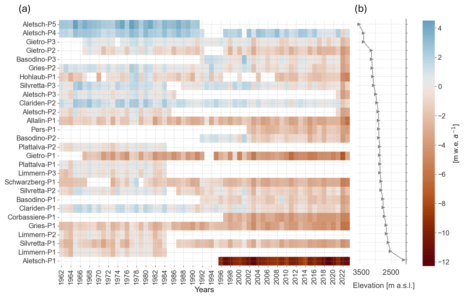
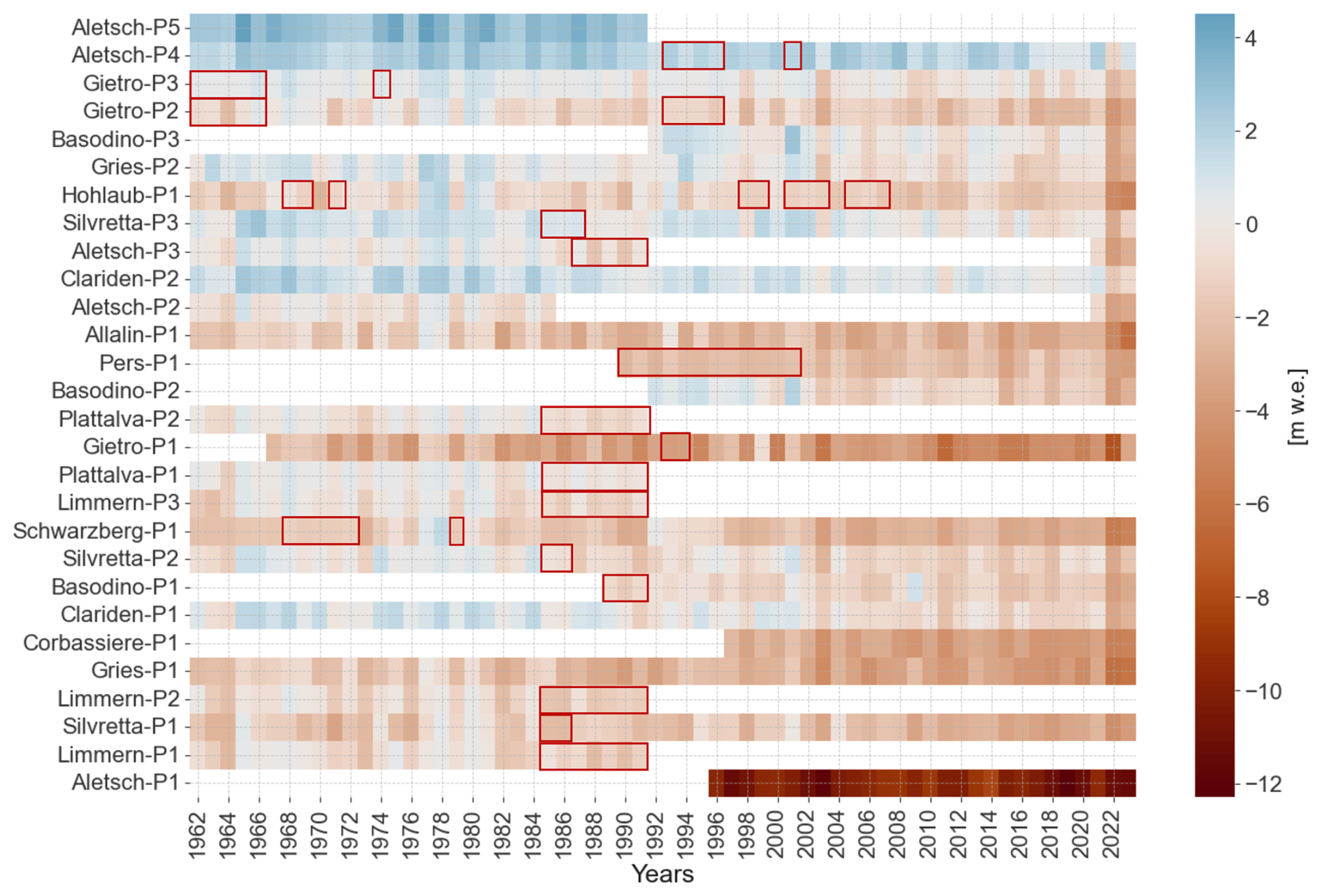
Figure 2 (a) Annual point surface mass balance (PMB) measurements by the Glacier Monitoring in Switzerland (GLAMOS) network at 28 sites on 13 glaciers from 1961 to 2023. PMB measurements range from −12.3 to +4.49 m w.e.; the sites are selected to have at least 20 years of (possibly non-consecutive) measurements and are ordered from low (bottom row) to high (top row) elevation. (b) Elevation of sites, ranging from sites Aletsch-P1 at 2089 $\mathrm{m}\mathrm{a}.\mathrm{s}.\mathrm{l}$ to Aletsch-P5 at 3526 $\mathrm{m}\mathrm{a}.\mathrm{s}.\mathrm{l}$.

The extensive spatio-temporal coverage of on-site PMB measurements in Switzerland is unique on a global scale. Over a century of continuous monitoring has been dedicated to a subset of glaciers, with 20 glaciers having over 30 years of data. Measurements are made with stakes relocated to their initial position annually, recording their height above the surface at specific intervals, supplemented with density measurements (Huss and Bauder, 2009). These field observations are affected by inconsistent measurement dates due to weather and other constraints. Typically, two surveys are conducted annually: one close to maximum snow depth to measure the winter MB around 30 April, with a standard deviation (SD) of 10 d, and one near the end of the melting season to determine the summer and annual PMB (30 September ± SD of 11 d). For detailed information on the dataset and its collection, refer to Geibel et al. (2022).

Here, we rely on a curated PMB dataset for selected long-term sites, with all observations homogenised to the hydrological year from 1 October to 30 September of the following year. For the homogenisation of raw field measurements, an approach proposed by Huss and Bauder (2009) was used to account for and correct for the differences between measurement dates for winter and/or annual MB and the hydrological year. A daily accumulation and positive degree-day melt model (Hock, 1999) is fitted annually to the seasonal data of each selected point measurement site (see also Huss et al., 2021). This results in a daily dataset of modelled MB that agrees with seasonal in situ observations and allows PMB to be extracted for the hydrological year.

For this study, we selected sites with a minimum of 20 years of non-consecutive measurements since 1961 (start of the gridded meteorological MeteoSwiss dataset), resulting in 1145 PMB measurements in total (Fig. 2a). Five sites have complete time series of PMB measurements from 1961 to 2023 (Clariden-P1 and P2, Allalin-P1, Gries-P1 and P2), while the others either have shorter series spanning 20–30 years or contain gaps. Given that miniML-MB is trained on individual sites, we train the ML model on datasets comprising a maximum of 60 (62) points from 1961 to 2021 (2023), depending on whether extreme MB years are included.

3 Machine-learning model

This study presents miniML-MB, a minimal ML model that aims to predict annual PMB for a specific location i on a glacier using information from meteorological variables. miniML-MB is trained separately for each site and builds a regression model that estimates the function f_i, fulfilling

$$\begin{array}{}\text{(1)}& \mathit{y}=f_i\left(\mathit{X}\right),\end{array}$$

where y is the annual observed PMB covering N hydrological years, and X is a predictor array made from temperature and precipitation variables.

3.1 Experiments with the model's input

miniML-MB faces the challenge of being trained on very small datasets which reflect realistic conditions in glaciology, with stake measurements in other parts of the world typically containing even less data than Switzerland's long-term glacier record. Working with glacier PMB series for single sites requires an ML setup tailored to handle such small datasets. This data-limited scenario poses a difficulty for ML models as their ability to discern patterns is typically correlated with the dataset size (Bottou and Bousquet, 2011). Additionally, ML models have to address the curse of dimensionality (Peng et al., 2024). This refers to the phenomenon where, as a model's number of features (dimensions) increases, the amount of data required to construct reliable models grows exponentially. Mitigating this issue typically involves reducing the dimensionality of the input feature space, which, in our case, means that miniML-MB should aim to capture most of the observed PMB variability using as few predictor variables as possible. In our analysis, we study the effect of relying on a varying number of predictors and explore which options optimally represent the meteorological information necessary to predict PMB.

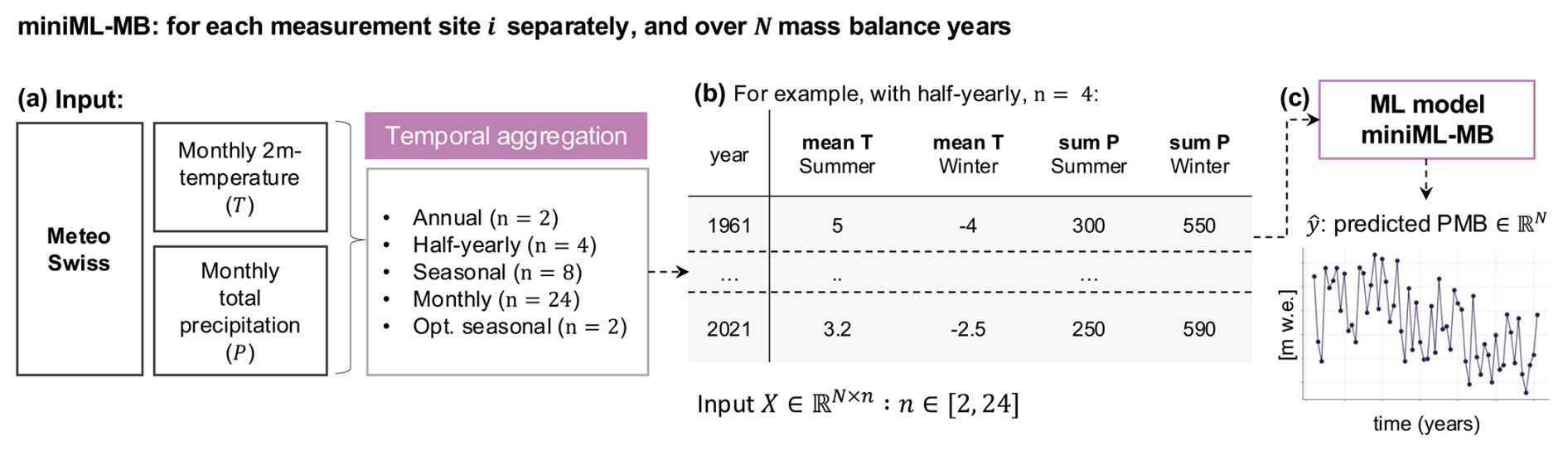
Figure 3 Conceptual overview of the training of miniML-MB, the point surface mass balance (PMB) machine-learning (ML) model. For each PMB measurement site i, miniML-MB is trained to simulate PMB from meteorological variables. (a) Pre-processing of monthly air temperature (T, in °C) and total precipitation (P, in $\mathrm{m}\mathrm{w}.\mathrm{e}.$) from MeteoSwiss. (b) Meteorological variables are formed into X, an array of N rows (number of annual PMB measurements at the site) and n columns (number of predictors). This example shows X during half-yearly aggregation with four predictors (n=4, summer and winter half-years). (c) X is given as input to miniML-MB, which predicts PMB $\widehat{\mathit{y}}$ covering N years.

To reduce the predictor space of miniML-MB, we rely on temporal aggregations of monthly climatic data. Here, the input features X of miniML-MB for a site are given as an array of dimension N×n (Fig. 3b), where N is the number of annual PMB observations, and n is the number of predictors made from aggregates of temperature and precipitation (ranging between 2 and 24). These aggregates are computed from monthly MeteoSwiss measurements using the mean for temperature and the sum for precipitation. We explore four levels of temporal aggregation (Fig. 3a):

1. Annual. The predictors are the mean annual temperature and total annual precipitation over the hydrological year (2 predictors, n=2).

2. Half-yearly. The predictors are the winter (October–March) and summer half-years (April–September) (n=4).

3. Seasonal. The predictors are the four glaciological seasons, namely April–June, July–September, October–December, and January–March (n=8).

4. Optimal seasonal. This is made up of two predictors (n=2), one for temperature and one for precipitation, aggregated over consecutive months (max. 6), for example, mean temperature from October to January and total precipitation from February to April. The idea of this setup is to use a flexible construction of seasons, where the information of months driving PMB might reside in intervals that overlap with seasons and/or are smaller than half-years. We limited the maximum number of consecutive months to 6 because extending beyond this threshold risks diluting the relevant information needed to predict PMB accurately.

5. Monthly temperature and precipitation (n= 24). This setup has the largest number of predictors.

3.2 Architecture

The ML architecture used in miniML-MB is eXtreme Gradient Boosting (XGBoost) (Chen and Guestrin, 2016). This open-source supervised-learning model consists of an ensemble of decision trees relying on two principal concepts: (i) a regularised learning objective, which reduces overfitting by penalising complex models, and (ii) gradient boosting. Gradient boosting iteratively improves the model's performance by additively building trees during training to reconstruct the difference between observed and predicted data (Friedman, 2001).

Our setup is one of sparse data consisting of heterogeneous features with generally small sample sizes (maximum of 60 years of measurements per site), structured in a tabular format (Fig. 3b). For tabular data, tree-based models like XGBoost are among the best-performing approaches, particularly for small- to medium-sized datasets, as demonstrated in benchmarking studies (e.g. Grinsztajn et al., 2022; Xu et al., 2021). Furthermore, since we aim to reconstruct PMB through a simple and interpretable approach, XGBoost is an ideal candidate as it is typically faster to train, needs less feature engineering, and is more interpretable than neural networks (Grinsztajn et al., 2022).

3.3 Training and testing

Determining the predictive performance of miniML-MB requires an evaluation of the model's predictions made on an independent test dataset. For ML models, this is usually done by splitting a dataset into training and testing sets. Given the small dataset size per site, allocating more data points for the test set risks reducing miniML-MB's predictive power by shrinking the training set, even though performance estimation improves. As a trade-off, we adopt a cross-testing framework, sometimes referred to as nested cross-validation, by using the entire dataset for both independent testing and hyperparameter tuning. During this framework, in independent testing, the dataset is shuffled and split into five folds (subsets) (Fig. 4a). Each fold is used once as an independent “test set”, unseen by miniML-MB during training, while the model is trained (or “fitted”) on a “training set”, which is the remaining aggregate of folds (hyperparameter tuning; see below). This process is repeated five times until miniML-MB has made predictions for each test set, and these are aggregated to recreate a time series covering each year for which PMB measurements were taken (Fig. 4b). The performance of miniML-MB is evaluated by comparing its predicted PMB time series to the observed PMB in terms of precision using the mean absolute error (MAE), root mean square error (RMSE), and temporal synchronicity using Pearson's correlation.

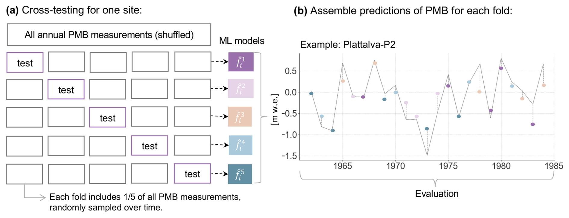
Figure 4 Testing framework of miniML-MB illustrated at site P2 on the Plattalva glacier. (a) At each point surface mass balance (PMB) measurement site i, miniML-MB makes PMB predictions, which are then evaluated using a cross-testing framework. Input climate predictors and observed PMB measurements are divided into five subsets. Five times, miniML-MB is trained on four of these subsets and makes predictions on the remaining (unseen) test subset. (b) The predictions made on these five test subsets (one coloured dot per subset) are aggregated to reconstruct a PMB time series for the site, covering all years with observed data. The accuracy of these predictions is assessed against the observed PMB (grey line).

The training process is controlled by different hyperparameters, i.e. external configuration variables manually set before training a model. To find the ensemble that gives the best model, we perform a randomised grid search based on the following hyperparameters: learning rate $\in [\mathrm{0.01},\mathrm{0.2}]$, the number of estimators $\in [\mathrm{50},\mathrm{300}]$, and the maximum depth $\in [\mathrm{3},\mathrm{10}]$. During the randomised grid search, a fixed number of hyperparameter sets is sampled from the specified ranges, and each set is evaluated using cross-validation in the independent testing component: the training set from above (not the original or entire dataset) is randomly separated into five folds. Five times, miniML-MB is trained on four folds and validated based on the remaining fold (the “validation set”), giving a validation loss. The optimal hyperparameters give the smallest average validation loss over all folds. miniML-MB is then fitted to the training set using the optimal set of hyperparameters, and predictions are made on the independent test set (see previous paragraph). With cross-testing, the hyperparameter search is less likely to overfit the dataset because it is only exposed to a subset of the data from the independent testing component of the cross-testing framework.

During miniML-MB's fitting to the training set, the model is configured to minimise its MAE loss function. We chose the MAE because of strong intra-site variability in PMB, especially at sites with long measurement series and because the MAE is more robust to outliers. Initially, we used the MSE as the loss function, but switching to MAE resulted in a slight performance improvement, though the change was not drastic.

Fitting miniML-MB to the training dataset using a GPU (NVIDIA GeForce RTX 2070) takes approximately 5 min for all 28 sites or 10 s per site on average; predictions are virtually instantaneous.

4 Positive degree-day model baseline

Our PMB predictions with miniML-MB are compared with those from a positive degree-day PMB model (PDD model in the following). For the latter, we rely on a simplified version of the SMB module from the Global Glacier Evolution Model (GloGEM,  Huss and Hock, 2015) that calculates the mass balance for a given elevation band based on a PDD implementation for melt and a simple temperature threshold for accumulation. The equations and parameters below are sourced from Huss and Hock (2015).

4.1 Implementation of the PDD model

For each PMB measurement site i, the steps below are repeated for every month m of a hydrological year.

1. Air temperature at the site T_i,m (°C) is extrapolated from the temperature of the MeteoSwiss reanalysis grid cell that covers the site T_cell,m:

   $$\begin{array}{}\text{(2)}& T_{i,m}=T_{\mathrm{cell},m}+(z_i-z_{\mathrm{cell}})\cdot \mathrm{d}T/\mathrm{d}z,\end{array}$$

   where z_i and z_cell are the elevation (m) of the site and the mean elevation of the reanalysis grid cell, respectively, and $\mathrm{d}T/\mathrm{d}z$ is a temperature gradient between −0.65 and −0.5 °C per 100 m. This gradient depends on the site and month and is calculated from ERA5-Land air temperatures at different pressure levels (not available for MeteoSwiss).

2. Monthly PDD temperature at the site $T_{i,m}^{+}$ is calculated from daily MeteoSwiss air temperature as follows:

   $$\begin{array}{}\text{(3)}& T_{i,m}^{+}=\sum _{d\in D}{T}_{i,d}^{+},\end{array}$$

   where D is the number of days in the month, and $T_{i,d}^{+}$ is the mean daily temperature, extrapolated to the site's elevation, for days d where the temperature was positive. $T_{i,d}^{+}=\mathrm{0}$ for days with a mean temperature below 0.

3. Ablation at the site a_i,m ($\mathrm{m}\mathrm{w}.\mathrm{e}.$) is calculated from $T_{i,m}^{+}$:

   $$\begin{array}{}\text{(4)}& a_{i,m}=\mathrm{DDF}\cdot T_{i,m}^{+},\end{array}$$

   where DDF is the degree-day factor ($\mathrm{m}{\mathrm{d}}^{-\mathrm{1}}\mathrm{°}{\mathrm{C}}^{-\mathrm{1}}$) to be calibrated (see Sect. 4.2). DDF is dependent on the current surface type (see step 6), with lower values for snow-covered surfaces (DDF_snow) and higher values for ice-covered surfaces (DDF_ice). The relation between the two DDFs is fixed (${\mathrm{DDF}}_{\mathrm{ice}}=\mathrm{2}\cdot {\mathrm{DDF}}_{\mathrm{snow}}$) and is based on the literature (e.g. Hock, 2003).

4. Precipitation at the site P_i,m ($\mathrm{m}\mathrm{w}.\mathrm{e}.$) is extrapolated from the MeteoSwiss reanalysis grid cell that covers the site P_cell,m:

   $$\begin{array}{}\text{(5)}& P_{i,m}=P_{\mathrm{cell},m}\cdot {\mathbf{c}}_{\mathrm{prec}}\cdot (\mathrm{1}+(z_i-z_{\mathrm{cell}})\cdot \mathrm{d}P/\mathrm{d}z),\end{array}$$

   where c_prec is a precipitation correction factor to be calibrated (see Sect. 4.2), and $\mathrm{d}P/\mathrm{d}z$ is a precipitation lapse rate set to 1 $\mathrm{m}\mathrm{w}.\mathrm{e}.{\mathrm{m}}^{-\mathrm{1}}$.

5. Accumulation at the site c_i,m ($\mathrm{m}\mathrm{w}.\mathrm{e}.$) is computed from monthly precipitation by applying a temperature threshold of T_thresh=1.5 °C and a gradual transition between the solid and the liquid phase in the range of T_thresh±1 °C.

   $$c_{i,m}=\left\{\begin{array}{ll}{P}_{i,m},& \text{if }{T}_{i,m}\le T_{\mathrm{thresh}}-\mathrm{1}\\ P_{i,m}\cdot \mathrm{1}/\mathrm{2}\cdot (T_{\mathrm{thresh}}+\mathrm{1}-T_{i,m}),& \text{if }{T}_{\mathrm{thresh}}-\mathrm{1}<T_{i,m}<T_{\mathrm{thresh}}+\mathrm{1}\\ \mathrm{0},& \text{if}{T}_{i,m}\ge T_{\mathrm{thresh}}+\mathrm{1}\end{array}\right.$$

6. With regard to surface type and snow depth, the surface is considered to be snow-covered as long as the snow depth s_i,m (m) is above 0 m. Otherwise, the surface type is bare ice. The snow depth is set to zero at the beginning of each hydrological year and is updated each month using the difference between computed accumulation and ablation:

   $$\begin{array}{}\text{(6)}& s_{i,m}=max\left(\mathrm{0},s_{i,m-\mathrm{1}}+c_{i,m}-a_{i,m}\right).\end{array}$$

7. With regard to the PMB update, monthly PMB at a stake location b_i,m ($\mathrm{m}\mathrm{w}.\mathrm{e}.$), set to zero at the beginning of each hydrological year, is calculated as the difference between accumulation and ablation:

   $$\begin{array}{}\text{(7)}& b_{i,m}=b_{i,m-\mathrm{1}}+c_{i,m}-a_{i,m}.\end{array}$$

4.2 Calibration and evaluation of the PDD model

The PDD model needs a calibration of the parameters c_prec and DDF_snow for each site and hydrological year. First, c_prec is calibrated against observed winter PMB using a predefined value for DDF_snow. Then, DDF_snow is calibrated against the observed annual PMB while using the value for c_prec determined in the first step.

More precisely, for each year, the PDD model will first predict cumulative PMB from October to April with all $c_{\mathrm{prec}}\in [\mathrm{0.8},\mathrm{4}]$ and a fixed DDF_snow of 3 $\mathrm{mm}\mathrm{w}.\mathrm{e}.{\mathrm{d}}^{-\mathrm{1}}\mathrm{°}{\mathrm{C}}^{-\mathrm{1}}$ (chosen based on the literature; Huss and Hock, 2015; Braithwaite, 2008) until the model matches the observed winter PMB. If there is no match, the parameter giving the closest value to the observed winter PMB is chosen. In a second step, the model predicts cumulative PMB from October to September using the optimal c_prec found in the first step and varying DDF_snow between 1 and 10 $\mathrm{mm}{\mathrm{d}}^{-\mathrm{1}}\mathrm{°}{\mathrm{C}}^{-\mathrm{1}}$ until a match with the annual observed PMB is achieved. In this case, too, the parameter that gives the annual PMB closest to the target is selected if no match is found.

This procedure is repeated for every year in the calibration period, creating a yearly parameter set. These parameters are then averaged when making predictions on the test dataset. The PDD model is cross-tested like miniML-MB, meaning that the calibration procedure is repeated five times for each site (five independent test folds) to make predictions for the whole dataset. The PDD model is evaluated following the same metrics as miniML-MB (see Sect. 3.3).

5 Results

5.1 Variable selection for optimal-seasonal framework

A comprehensive analysis is conducted to find the best combination of months for both temperature and precipitation to run miniML-MB in the optimal-seasonal framework (see Sect. 3.1). To this end, miniML-MB is run with all possible combinations of up to 6 consecutive months for temperature (T[month_i to month_j]) and precipitation (P[month_m to month_n]), resulting in a total of 3249 combinations. An analysis of the distribution of average validation MAE over all sites for each combination shows a left-skewed pattern, with values ranging from 0.575 to 0.974 m w.e. (Fig. 5a). Here, we analyse the validation MAE calculated in cross-testing – not the test MAE – to avoid overfitting and because hyperparameters should not be selected based on the independent test set. The combination yielding the lowest MAE is T[April–August] and P[October–February], with several other combinations having a relatively small validation MAE too. Following Zekollari and Huybrechts (2018), we select the 1 % (33) and 50 best combinations with the lowest average MAE over all sites (purple and yellow panels in Fig. 5a). Within this selection, we analyse the frequency of occurrence of individual months (Fig. 5b–e), computed as the number of times a month appears in the selection divided by the number of combinations in the ensemble.

Figure 5 Feature importance of miniML-MB. (a) Histogram of validation MAE by miniML-MB averaged over all 28 sites and calculated for all possible combinations of contiguous (max. 6) months. The purple and yellow areas indicate, respectively, the 1 % (33) and 50 best combinations, i.e. the lowest average validation MAE over all sites. The dashed grey line shows the average MAE over all sites (0.7 m w.e.) obtained if miniML-MB predicted, for each year, the average PMB measured at each site. Frequency of temperature and precipitation in the (b–c) 1 % best and (d–e) 50 best combinations. The frequency is calculated as the number of times a month is present divided by the number of combinations in the best ensemble.

For temperature, the frequency of months in the 1 % and 50 best combinations are very similar (Fig. 5b, d). June appears in all combinations, while May, July, and August are present in over half of the best combinations. April and September are present in approximately one-third of the combinations. The influence of temperature on PMB in other months appears to be very small to negligible since these months are rarely present in the combinations that yield low MAEs. Regarding precipitation, all months are represented across the best combinations (Fig. 5c, e). However, the period of October through January, which marks the onset of the accumulation season, stands out, with frequencies surpassing 0.5 (i.e. present in more than 50 % of all combinations). February and March also exhibit high occurrence rates, while precipitation during spring and summer seems to have less impact on PMB.

Because of this result, for the optimal-seasonal framework that relies on two predictors only, we select the average air temperature from May to August (T[May–August]) and the total precipitation from October to February (P[October–February]).

5.2 Performance of miniML-MB with different predictors

We trained miniML-MB with various temporal resolutions of temperature and precipitation (see Sect. 3.1): (i) annual (2 predictors), (ii) half-yearly (4 predictors), (iii) seasonal (8 predictors), (iv) monthly (24 predictors), and (v) optimal seasonal (2 predictors, namely T[May–August] and P[October–February]). Here, we assess the impact of these different predictors on miniML-MB's ability to predict PMB by comparing average test metrics across all sites (Fig. 6).

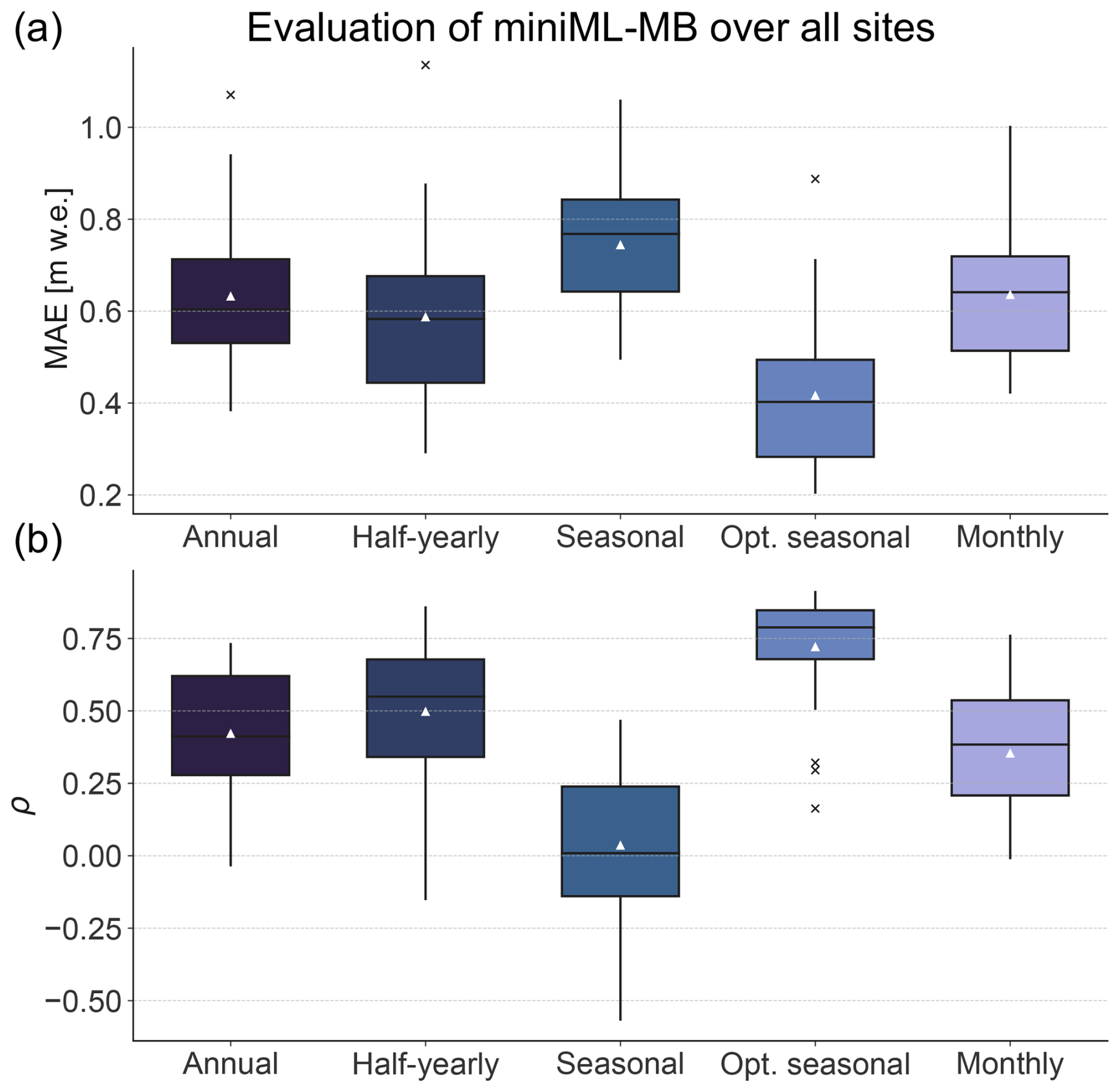
Figure 6 Performance of miniML-MB assessed with different temporal resolutions of predictors. The predictors consist of various temporal aggregates of temperature T and precipitation P: (from left to right) annual, half-yearly, seasonal, optimal seasonal (T[May–August] and P[October–February]), and monthly (see Sect. 2.1). (a) Mean absolute error (MAE) and (b) Pearson's correlation coefficient ρ are calculated between predicted and observed point surface mass balance with cross-testing (see Sect. 3.3). The boxplots represent the distribution of these evaluation metrics across all sites. The boxes show the quartiles, while the whiskers extend to the rest of the distribution (black line for median and white triangle for mean), excluding outliers (crosses).

Increasing the number and temporal resolution of predictors, e.g. going from annual to monthly predictors, does not improve the model's capability to predict PMB in terms of both MAE and Pearson correlation. This contrasts with typical ML approaches, where a larger number of candidate features is generally preferred, as the model automatically selects those with high explanatory power while disregarding those with little impact. In our case, miniML-MB does not seem to benefit from expanding the number of predictors. We suspect that this outcome is linked to the relatively small training dataset, which favours a low-complexity model with few but relevant predictors capturing most of the observed PMB variability. This is reflected in the fact that the optimal-seasonal aggregate outperforms other temporal aggregations for most sites, with a median MAE of 0.4 m w.e. and a median correlation of 0.8, while other aggregations have median MAEs of around 0.6–0.8 m w.e. and median correlations below 0.6 (Fig. 6). Notably, the range of correlation values across sites is narrower for the optimal-seasonal aggregate than the other aggregations.

These results illustrate the need for dimensionality reduction when dealing with small PMB datasets. The best results are achieved using two predictors based on temperature and precipitation after reducing the predictor space to include only the most relevant months. Interestingly, these predictors mimic the input data of a PDD model, which is generally suitable to operate under these types of conditions.

5.3 Benchmarking miniML-MB against a PDD model

In this section, we compare miniML-MB in the optimal-seasonal framework with the PDD model presented in Sect. 4.

The PMB predicted for 1961–2021 by miniML-MB is generally closer to observations than the PDD model (Fig. 7a), with notable differences in average MAE (0.417 m w.e. for miniML-MB versus 0.541 m w.e. for the PDD model) and RMSE (0.604 m w.e. versus 0.687 m w.e.). The models' performances are almost identical in terms of correlation, with average Pearson's correlations of 0.72 and 0.73.

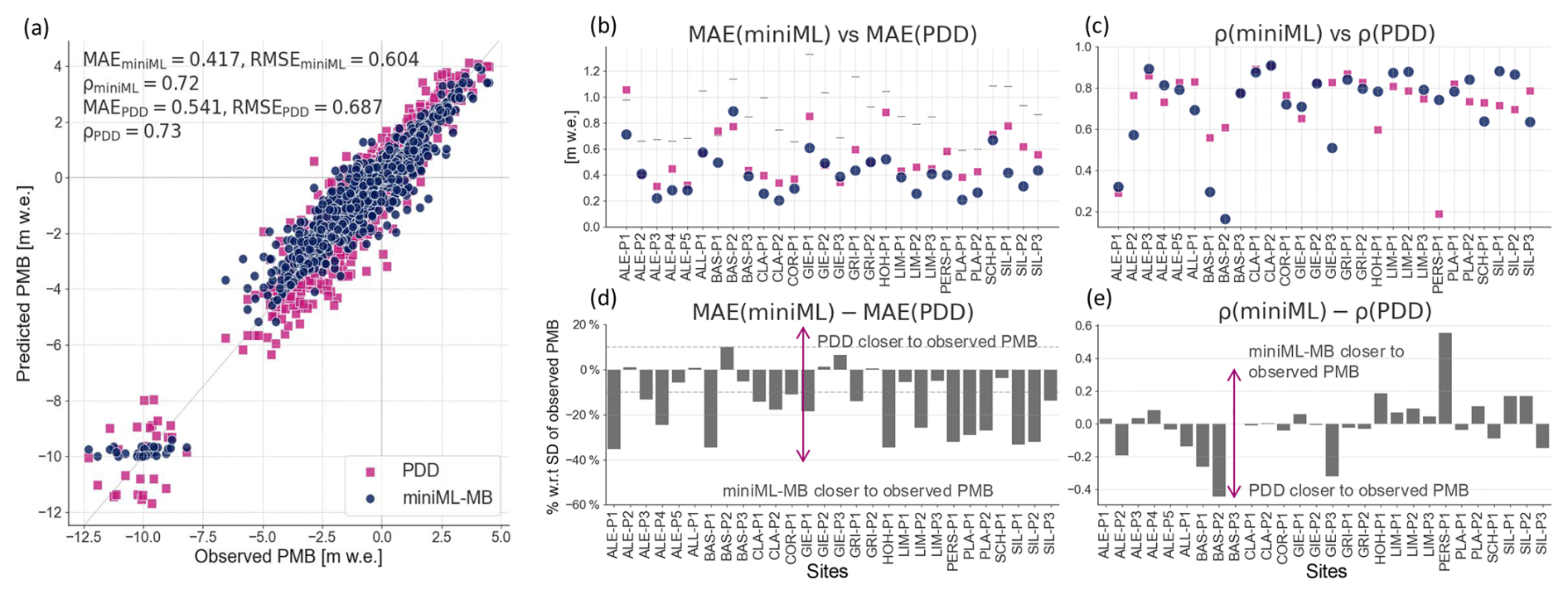
Figure 7 Performance of miniML-MB (blue dots) and PDD model (pink square) compared to observed point surface mass balance (PMB) time series. miniML-MB is trained within the optimal-seasonal framework using two predictors from temperature T[May–August] and precipitation P[October–February]. (a) Observed versus predicted PMB by both models for all 28 glacier sites. Average evaluation metrics over all sites are calculated between predicted and observed PMB time series (see Sect. 3.3): mean absolute error (MAE), root-mean-square error (RMSE), and Pearson's correlation ρ. (b, c) Evaluation metrics for both models for each site. Every site in (b) also contains the standard deviation (SD) of the observed PMB time series (horizontal grey lines). (d, e) The difference in evaluation metrics between both models for each site. For (d), the difference in MAE is expressed in terms of percentage with respect to the SD of the observed PMB.

More precisely, the PMB predicted by miniML-MB is closer to the observed PMB than the PDD model for 22 out of 28 sites (Fig. 7b, d). These differences are relatively marked, with six sites having a difference in MAE larger than 30 % of the SD of the observed PMB, nine sites having differences above 20 %, and 17 sites having differences above 10 %. This is illustrated with five examples of time series with various temporal patterns: Plattalva-P2, Silvretta-P2, Clariden-P2, Aletsch-P4, and Hohlaub-P1 (Fig. 8a–e). For each of these five sites, except for a few single years, miniML-MB comes very close to reproducing the temporal patterns of the observed PMB series in terms of both accuracy (MAE around 0.2–0.3 m w.e., except for Hohlaub-P1, with 0.5 m w.e.) and temporal synchronicity (Pearson's correlation from 0.8 to 0.9). For these sites, miniML-MB also strongly outperforms the PDD model in terms of MAE (difference in MAE of 20 % to 30 % w.r.t. the SD of the observed PMB).

Regarding temporal synchronicity, the Pearson's correlation varies depending on the site, but, on average, both miniML-MB and the PDD model exhibit similar performances (Fig. 7c, e). Roughly half of the sites have a higher correlation with observed PMB for miniML-MB compared to the PDD model and vice versa. This is also reflected in the sites' year-to-year variabilities (Fig. A1 in the Appendix): miniML-MB's predictions have a smaller SD than the one of observed PMB, while the PDD model tends to overestimate variability.

One site stands out due to its low Pearson's correlation and high MAE: the low-altitude site Aletsch-P1, with extremely negative annual PMB (Fig. 8f and dots in the lower quadrant of Fig. 7a). For this site, both miniML-MB and the PDD model struggle to accurately fit the observed PMB, with MAEs of 0.71 and 1.05 m w.e., respectively. miniML-MB predicts almost constant PMB values around −10 m w.e. for all years. The combination of very negative PMB and a short time series (20 years) might mean insufficient data for the models to learn the site's characteristics. Since the months of the optimal-seasonal framework are chosen based on results averaged over all stakes, it is also possible that they may not capture the most relevant PMB drivers for this particular outlier site. To accurately model Aletsch-P1, more data, different feature engineering, or additional meteorological features (like albedo, for example) may be required.

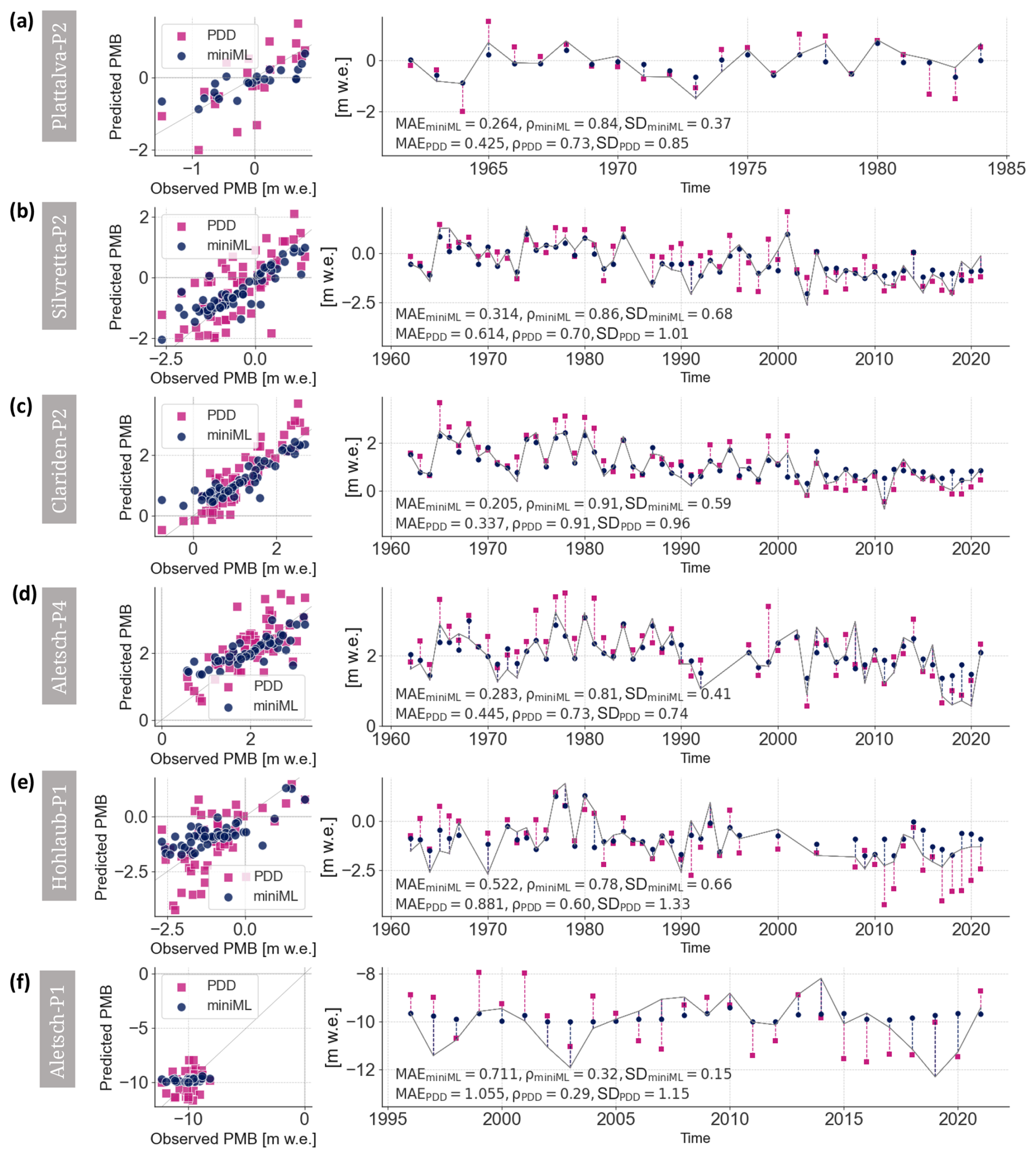
Figure 8 Examples of point surface mass balance (PMB) predictions made by miniML-MB (blue dots) and PDD model (pink square) for six sites: (a) Plattalva-P2, (b) Silvretta-P2, (c) Clariden-P2, (d) Aletsch-P4, (e) Hohlaub-P1, and (f) Aletsch-P1. Each panel shows a scatterplot of (left) modelled vs. predicted PMB and (right) a time series compared to observed PMB (grey lines). Evaluation metrics of mean absolute error (MAE), Pearson's correlation ρ, and standard deviation (SD) are calculated between predicted and observed PMB time series.

5.4 Prediction of extreme years

So far, the extreme years of 2022 and 2023 were excluded from the analyses. During these years, Swiss glaciers lost 10 % of their total volume (6 % in 2022 and 4 % in 2023) (GLAMOS, 2023b) due to low-accumulation winters and exceptionally high spring and summer temperatures (SCNAT, 2023; Cremona et al., 2023). In 2022 (2023), 18 (10) out of the 20 sites had a PMB that was lower than in any other year before 2021. These sites with extreme mass loss are highlighted in purple in Fig. 9.

Here, we evaluate miniML-MB's ability to predict the PMB of extreme years. First, we assess if miniML-MB, trained with data up to 2021, could predict the PMB for 2022 and 2023 (Figs. 9a and A2). Then, we trained the model with data up to 2022 to predict the PMB for 2023, assessing the impact of including one extreme year in the training dataset (Fig. 9b). Both miniML-MB and the PDD model were trained and tested with data from 2022 and/or 2023 without cross-testing.

miniML-MB is not able to correctly predict 2022's PMB. PDD model's predictions are closer to the observed PMB for all sites (Fig. 9a), with a difference in MAE above 50 % with respect to the SD of the observed PMB, except for Aletsch-P1, where 2022 was not an extreme event. In contrast, for 2023, miniML-MB trained with data until 2021 predicts a PMB closer to observed values than the PDD for 11 of the 20 sites (Fig. 9b), with differences above 50 % with respect to the SD of the observed PMB. For these 11 sites, only Gries-P1 and Gries-P2 had an extreme 2023 year. Including 2022 in the training dataset improves miniML-MB's 2023 predictions for all sites where 2023 was an extreme year (Fig. 9b).

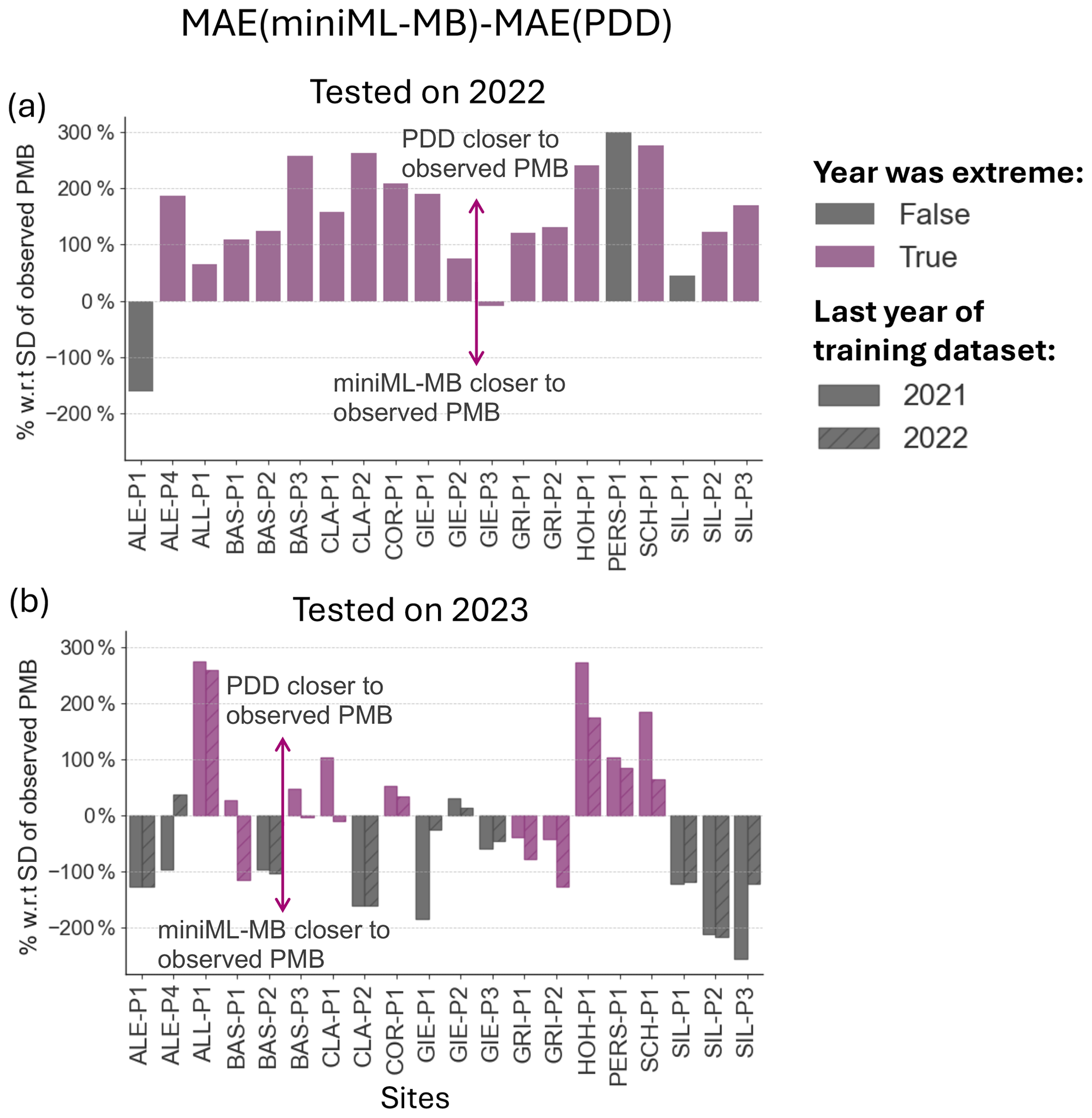
Figure 9 Predictions of 2022 and 2023 extreme years by miniML-MB compared to the PDD model for 20 sites. In (a), the models are trained with time series that end in 2021 and are tested on 2022. In (b), the models are trained with time series that end in 2021 (no hash) or 2022 (diagonal hash) and are tested on 2023. Sites for which 2022 or 2023 were extreme, i.e. where observed PMB values had not been observed before 2021, are coloured in purple.

These and previous results show that miniML-MB seems to have good generalisation abilities, meaning that the model can adapt to unseen data drawn from a similar distribution as the training data (Figs. 7 and 9b for non-extreme years). However, for both extreme years, miniML-MB's predictions saturate by converging to an almost constant value, within the range of observed PMB, that follows the site's trend of the last decade (Fig. A2). Since tree-based models split value ranges into different segments, when an extreme value is encountered, it falls into the outermost leaf of the tree, therefore saturating the response. Thus, while tree-based models excel at interpolation, they cannot produce values beyond those seen in the training dataset. Because 2023 was not a strong outlier for Gries-P1 and Gries-P2, this also explains why miniML-MB can forecast PMB values relatively accurately for these sites. Providing one extreme year in its training dataset already improves miniML-MB's performance in generalising to extreme years, highlighting its potential ability to learn rapidly. Our findings underscore the necessity for ML models to encounter temporal analogues in their training data in a climate that will exhibit increasingly extreme events. Once this is the case, miniML-MB shows promising abilities in making accurate PMB predictions for extreme years.

5.5 Gap filling with miniML-MB

We have shown that miniML-MB is capable of reconstructing PMB and of generating accurate predictions as long as predictions are made within a range of meteorological conditions seen in the training set. Here, we used miniML-MB to predict PMB for 17 sites with measurement gaps and to extend the tail or head of time series for years that have T[May–August] and P[October–February] within the site's observed range (Fig. 10). For example, Pers-P1 was extended from 1990 to 2001 because these years' temperature and precipitation predictors were within the range of MeteoSwiss values from 2002 to 2023. The values predicted for the filled gaps seem to follow the temporal trend of PMB for each site. As such, miniML-MB is a promising tool for filling gaps in PMB records. We do not recommend using the model to extrapolate outside the site's observed predictor values (e.g. filling Limmern-P2 from 1992 to the present) due to significantly different meteorological conditions compared to miniML-MB's training set.

Figure 10 Gap-filled version of Fig. 2. Initial gaps (highlighted by red rectangles) have been filled with results of miniML-MB trained within the optimal-seasonal framework.

5.6 Drivers of point surface mass balance

Through our custom dimensionality reduction framework, May to August (summer) temperatures and October to February (winter) precipitation are singled out as the main drivers for PMB (Fig. 5). The ability to identify key climatic drivers of PMB is an interesting feature of this ML approach. While predictors in a PDD model are grounded in established physical principles, statistical models like ML adopt an inverted approach. Instead of pre-selecting predictors and then simulating PMB, ML models work by directly identifying the most effective predictors from the available observations and data. Our results illustrate that this approach enhances performance by identifying the predictors that most effectively explain PMB observations in Switzerland. Consequently, these findings not only demonstrate the utility of this ML method but also help validate the climatic drivers of glacier MB commonly identified by glaciological studies (e.g. Braithwaite and Olesen, 1990; Chen and Funk, 1990; Greuell, 1992; Ohmura, 2001; Torinesi et al., 2002; Pellicciotti et al., 2005). The majority of studies investigating the relationship between temperature, precipitation, and SMB variations have consistently identified summer temperatures as the critical component. For instance, Oerlemans and Reichert (2000) quantified the climate sensitivity of a sample of glaciers worldwide and determined that summer temperature is the primary factor driving glacier-wide mass balance. In Switzerland, Zekollari and Huybrechts (2018) performed a regression study for PMB on the Morteratsch glacier complex (not included in our dataset) and found that the mean temperature from May to July and the total precipitation from October to February account for up to 85 % of the observed PMB variance.

Analysing the weights attributed to individual predictors in the optimal-seasonal framework for each site allows for a site-specific investigation of the monthly meteorological drivers of PMB. To this effect, we use a k-means++ clustering algorithm (Arthur and Vassilvitskii, 2007) to group sites according to the local importance of temperature and precipitation. Local feature importance is calculated for each site by taking the 50 combinations with the smallest MAE when running miniML-MB with all possible combinations of up to 6 months of temperature and precipitation (see Sect. 5.1).

The k-means++ clustering algorithm partitions the sites into three clusters. This number is chosen using the elbow method, i.e. by plotting the within-cluster sum of squares for various numbers of clusters and identifying the point of inflection of the resulting graph (Fig. A3). k-means++ separates the majority of sites (18) into one cluster (C1; Fig. 11a, d) and the remaining sites into two smaller clusters, each with five sites: C2 (Limmern-P1, Limmern-P2, Limmern-P3, Plattalva-P1, Plattalva-P2; Fig. 11b, e) and C3 (Aletsch-P4, Gietro-P1, Gietro-P2, Gietro-P3, Pers-P1; Fig. 11c, f). Compared to C1, which seems to be an ensemble of sites with diverse properties, C2 and C3 contain more specific features. C2 generally contains lower-elevation sites that are typically located close to the equilibrium line altitude, with mean PMB values around 0 m w.e. (Fig. 11i). These sites also have a shorter series of PMB observations, stopping in the 1980s (Fig. 11k, l). In contrast, C3 contains some higher-elevation sites, with PMB time series that span over longer periods and/or have more recent observations.

The frequency of “driving” temperature months has approximately the same pattern across all clusters (Fig. 11a–c). June and/or July emerge as the most important months, accompanied by a high frequency of occurrence for May and August. C1 seems to be dominated by the importance of temperature, with precipitation months having approximately the same weights (Fig. 11d). We suspect that this cluster regroups sites for which k-means++ found no distinguishing pattern in the importance of precipitation months. Therefore, we focus our analysis on C2 and C3. In C2, winter and spring temperatures also have some weight, which is not the case for C3 (Fig. 11b, c). There is also a strong contrast in the frequency of precipitation months (Fig. 11e, f). For C2, early-winter precipitation (October–January) determines the PMB, with frequencies > 0.6. For C3, late-winter and spring precipitation (February–June) have a higher weight.

In our site-specific analysis, early-winter precipitation emerges as a significant influence for sites with PMB data spanning from the 1960s to the 1980s and for data with PMB values close to zero. We suspect that accumulation had an important effect on annual PMB for these older and shorter records, explaining why winter precipitation stands out in cluster C2. On the other hand, summer temperatures are the predominant driver for PMB sites with longer and more recent data (C3). This might be due to steadily increasing summer temperatures, which outweigh the influence of precipitation and have lead to increasing glacier mass loss since the 1980s.

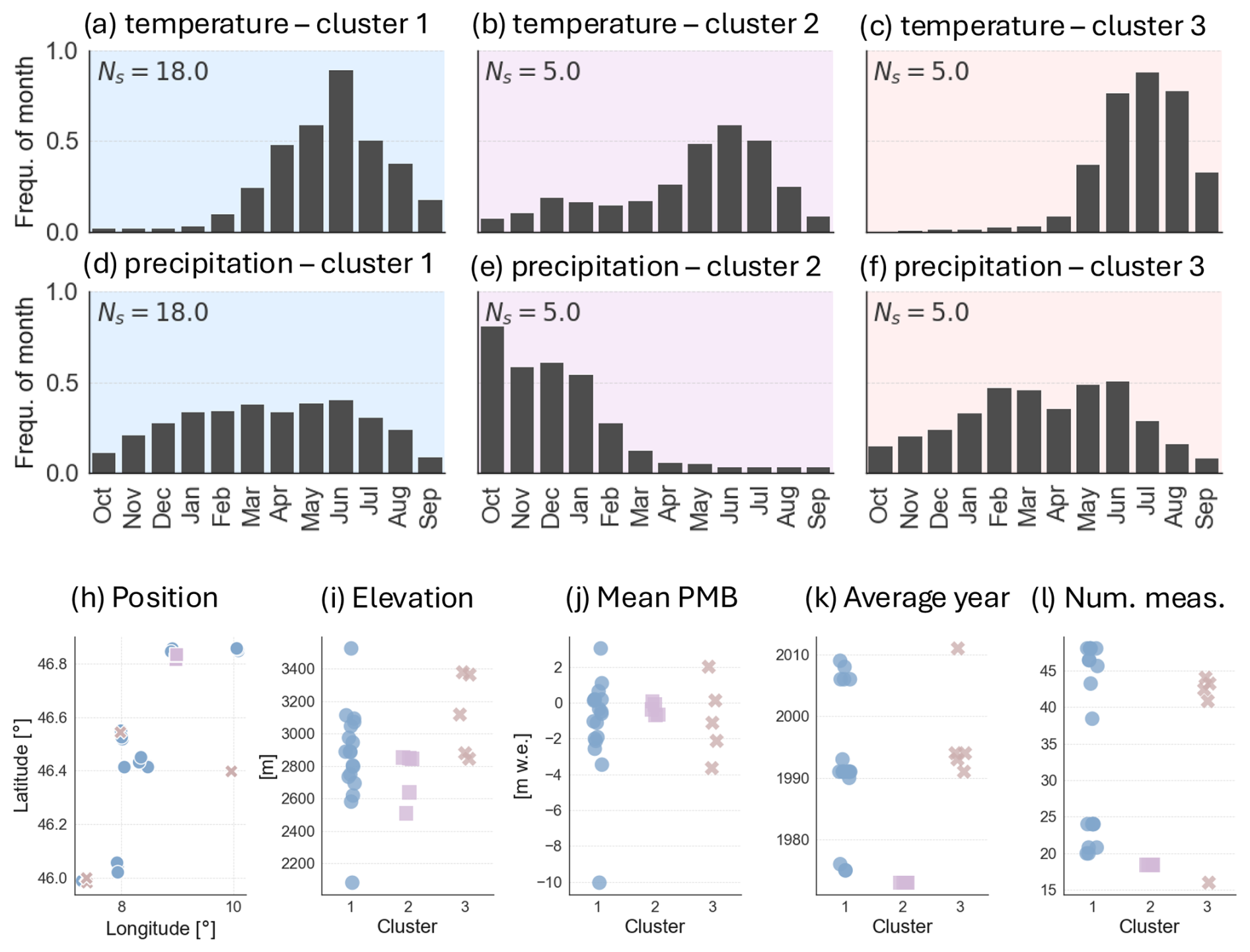
Figure 11 Clustering of sites according to the importance of monthly temperature and precipitation in predicting point surface mass balance (PMB). The k-means++ algorithm is used to group sites into three clusters: cluster 1 (blue), cluster 2 (pink), and cluster 3 (orange). (a–f) Mean frequency of temperature and precipitation months within each cluster, with N_s being the number of sites within each cluster. (h–l) Properties of sites, represented by colour-coded markers that refer to the specific cluster (cluster 1: blue dots, cluster 2: pink squares, and cluster 3: orange crosses). (h) Geographical latitude and longitude. (i) Elevation of the stake. (j) Mean observed PMB. (k) Average year of measurements. (l) Number of annual measurements.

6 Discussion

6.1 Source of meteorological data

We opted to utilise MeteoSwiss' reanalysis data instead of weather station data for several reasons. First, using a gridded product avoids the difficulty of selecting the most representative station for each site, thereby removing potential ambiguity. Second, gridded products reproduce the atmospheric conditions at any location, removing the need for spatial interpolation. Lastly, when considering potential applications to other regions, accessing gridded products is generally easier than obtaining representative station data. This flexibility also allows us to compare the effects of using a high-resolution dataset (such as MeteoSwiss) versus coarse-resolution climate reanalysis data (e.g. ERA5-Land; see below), providing insights into the generalisation to other regions. The gridded data by MeteoSwiss are available from 1961, meaning that some older PMB data cannot be included in the analysis. The effect is minor, though: 1476 PMB measurements are available from 1914 versus 1145 PMB measurements available from 1961.

The MeteoSwiss reanalysis data come in a high resolution (2 km), a level of detail not available in most other regions where miniML-MB could be applied. To assess the impact of utilising our detailed meteorological dataset, we replicated our analysis with ERA5-Land data (9 km resolution) for both miniML-MB with the optimal-seasonal framework and the PDD model (Fig. A4). While the overall performance is slightly superior with MeteoSwiss data, miniML-MB can still accurately predict PMB for most sites. Specifically, with ERA5-Land, miniML-MB outperforms the PDD model for 20 out of 28 sites (compared to 23 with MeteoSwiss), and 15 sites have a difference in MAE above 20 % with respect to the SD of observed PMB. This performance implies that miniML-MB could be readily employed with gridded products such as ERA5 or ERA5-Land for any other site globally.

6.2 Choice of meteorological variables and post-processing

We chose air temperature and total precipitation to drive miniML-MB for two main reasons: they are easily accessible and are typically used to describe PMB in numerical models. Glacier ablation is primarily influenced by longwave radiation and sensible heat flux, both of which are closely tied to air temperature variations (Hock, 2003). On the other hand, glacier accumulation generally happens in the form of solid precipitation (Huss and Bauder, 2009; Huss and Hock, 2015). More precisely, numerous studies have identified summer temperature and winter precipitation as the most important predictors of PMB (see Sect. 5.6). Furthermore, since miniML-MB can only utilise limited but concentrated information (see the optimal-seasonal framework designed for dimensionality reduction), we do not expect model improvement when adding additional meteorological variables such as shortwave or longwave radiation.

Initially, one might expect improved model performance when using predictors that are more deeply rooted in physical knowledge or that are less simple. To address this, we conducted additional evaluations of the model by incorporating more refined representations of temperature and precipitation. First, we used the sum of daily average temperatures above 0 °C in a month (PDD sums) instead of monthly average temperature, given how PDD sums are often more indicative of snowmelt and ice melt (Hock, 2003; Woul and Hock, 2005). However, the performance improvement in miniML-MB with the PDD sums was minimal to non-existent (Fig. A5a). It seems that miniML-MB is capable of effectively extracting relevant information related to melt processes by directly identifying patterns from the monthly input temperatures. Then, we used weighted mean air temperatures and precipitation totals, using weights based on the importance of months identified in Sect. 5.6: 0.58, 1.0, 0.56, and 0.52 for May to August temperatures and 0.52, 0.46, 0.6, 0.58, and 0.42 for October to February precipitation. Again, no performance improvement was observed (Fig. A5b). Our results demonstrate that more complex aggregations of temperature and precipitation offer limited to no added value in our minimal ML framework and support the need for dimensionality reduction instead. These findings suggest that the model acts as an “information compressor”, efficiently extracting the necessary information directly from the temperature and precipitation variables. This simplicity is, in fact, a key advantage, making the method more flexible and less reliant on extensive data.

6.3 Comparison with the PDD model

We have shown that, using just two predictors obtained through dimensionality reduction techniques, miniML-MB can closely match the PMB for individual glacier sites, surpassing the performance of the PDD model for most sites (see Sect. 5.3). Here, we discuss the question of whether comparing the two models is fair, given their essential differences and reliance on different predictors.

A fundamental difference between miniML-MB and the PDD model lies in their approach to modelling and understanding processes. ML methods are data-driven, relying on observational data to identify patterns and relationships without requiring physical principles or predefined rules (e.g. melt or snow threshold temperatures). These ML models are open-ended and flexible, adapting as more data become available, without a fixed structure or assumptions about the system. Importantly, they can still provide physically meaningful results, as shown in this study. In contrast, PDD models are mechanistic models based on established physical principles in glaciology. They have a fixed structure derived from these principles, making them less adaptable to data outside of their theoretical framework.

A natural consequence of their differing methodologies is that the models use different predictors. However, we believe that the validity of the comparison lies in ensuring that both models are tested on an independent dataset and calibrated under the same conditions (e.g. cross-testing). Under these criteria, the comparison remains robust and meaningful.

6.4 Limitations of miniML-MB

While data-driven methods for modelling PMB, such as miniML-MB, may complement traditional PDD models, the minimal ML approach we introduced also has important limitations.

While miniML-MB is generally able to accurately match the observed PMB and outperform the PDD model in terms of MAE for most sites, miniML-MB's year-to-year variability is generally much smaller than the observed one (Fig. A1). The reduced variability of miniML-MB could come from its loss function (MAE), which is not designed to account for temporal trends. The PDD model instead exhibits higher year-to-year variabilities, sometimes exceeding the observed one. As noted in other studies (e.g. Ismail et al., 2023; Bolibar et al., 2023), this may be because of the use of a fixed degree-day factor, which forces linearity. When values deviate from the main observations, non-linearities become more significant, potentially leading to overestimation or underestimation of the year-to-year variabilities. The underestimation by miniML-MB and the overestimation by the PDD model are respective drawbacks of the models.

ML models are highly specific, with their training datasets strongly determining their applicability. This is evident when using miniML-MB to predict extreme years (see Sect. 5.4). Our model struggles to extrapolate to values outside the range of the training data, such as those observed in 2022 and 2023. One reason for this is an inherent limitation of tree-based models as they rely on decision boundaries derived from the training data (Hengl et al., 2018). Another explanation might be that the drivers of PMB extracted through feature engineering might not be the same for a changing climate, meaning that the selection of optimal months might need to be repeated. However, our analysis shows that incorporating even 1 extreme year into the training dataset already enhances miniML-MB's predictive performance for most sites. While this finding is promising, training the ML model on an ensemble of sites could be an alternative by identifying extreme cases at other locations (i.e. capturing spatio-temporal analogues). Nonetheless, applying miniML-MB for future scenarios with extreme values will likely remain challenging.

While miniML-MB is designed for very small datasets through feature engineering, the requirement of 20 years of data per site is relatively long from a glacier monitoring perspective. Even though the framework does not require continuous PMB records, many glaciers worldwide lack such extensive records. This is a challenge for both miniML-MB and the PDD model, limiting the models' applicability to other sites. One advantage of miniML-MB is that it relies only on annual PMB. This is in contrast to the PDD model, which also needs seasonal PMB measurements, which are not readily available in many parts of the world. Calibrating both models with less data could be explored, but it would likely result in a biased calibration, impacting predictions (not tested here). ML could address this problem by using an ensemble of sites to train the model, where spatial analogues could be used. For example, grouping two or three nearby sites to create a dataset of at least 20 points could transfer some spatial properties while maintaining a relatively homogeneous dataset.

Due to the non-deterministic nature of XGBoost (and other ML algorithms), reproducibility depends on using the exact same settings (e.g. random seed provided as part of the code and data). This randomness primarily influences how the data are split into different folds during cross-testing. If this split is “unlucky”, the distribution of the validation or test folds might significantly differ from the training folds, resulting in a model that cannot learn the correct PMB relationship for a site.

7 Conclusions

This study developed miniML-MB, a novel data-driven approach to modelling PMB at stake locations. Based on the XGBoost architecture, the miniML-MB model was trained at individual PMB stake locations in the Swiss Alps, and its performance was compared to that of a PDD model.

miniML-MB is a highly computationally efficient ML model, making PMB predictions almost instantaneously. The model is streamlined for ease of use, with just three hyperparameters to adjust in its XGBoost architecture. Our data-driven approach is tailored to small observation datasets, a realistic context in glaciology but a technical challenge in ML. To ensure the best model performance, we implemented dimensionality reduction techniques to minimise the number of predictors. The best prediction performance of PMB was achieved through feature engineering by reducing the number of predictors of miniML-MB to two variables: mean air temperature from May to August and total precipitation from October to February. With these two predictors, miniML-MB can closely match the PMB for individual glacier sites, surpassing the PDD model for most sites as long as predictions are made within a range of meteorological conditions similar to the training set. While we have shown that a PDD model performs better for outliers such as the extreme years of 2022 and 2023, including just 1 extreme year in miniML-MB's training dataset already improves the model's predictive accuracy for most sites. While miniML-MB would ideally be exposed to multiple extreme cases to make predictions of future extreme years, this experiment highlights the model's potential for rapid learning.

Through our custom feature importance implementation, we quantify the significance of individual climate features. miniML-MB offered data-driven insights into the meteorological variables that drive local PMB, singling out mean air temperatures from May to August and total precipitation from October to February. More precisely, our site-specific analysis suggests that early-winter precipitation controlled PMB for sites with data from the 1960s to the 1980s and with PMB values close to equilibrium. For sites with longer and more recent data, summer air temperatures emerge as the predominant drivers of PMB. These findings align with the drivers of PMB identified in previous studies.

miniML-MB is tailored specifically to predict PMB and captures the characteristics of individual sites, enabling a site-by-site application. The model is a promising tool for efficiently providing local-scale information about PMB and its drivers and for filling gaps in the time series of measured PMB. At present, it is, however, unsuited for applications at the glacier-wide scale or for unseen sites. This would require training on an ensemble of sites to capture inter-site variability and is the focus of an ongoing follow-up study. While such a multi-site approach does not allow for site-specific optimisation, it has the potential to capture general trends across locations. Such an expansion to modelling an ensemble of sites will also come with new challenges, particularly as learning from small amounts of data and transferring knowledge to new domains remain difficult in machine learning (Dube et al., 2020).

In conclusion, this study introduces an innovative approach to PMB modelling while also underscoring potential improvements and more general applications for data-driven approaches in glaciology.

Appendix A

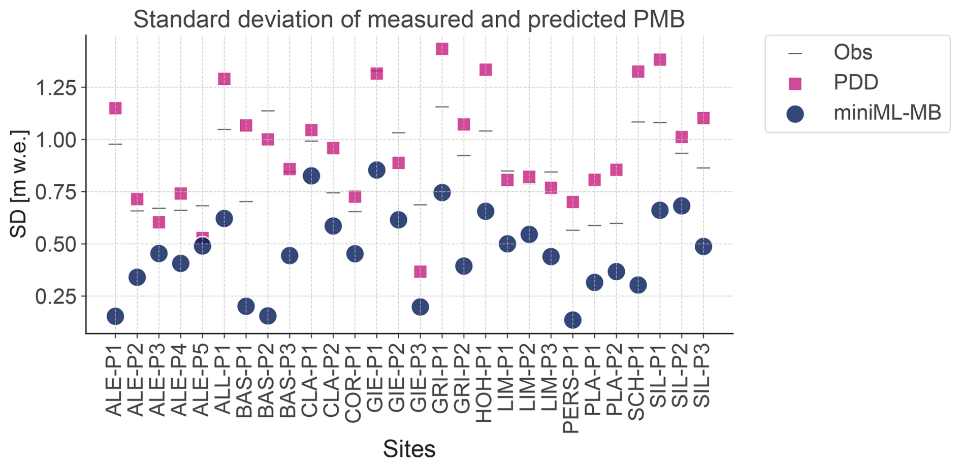
Figure A1 Standard deviations of point surface mass balance (PMB) predicted by miniML-MB (blue dots), trained within the optimal-seasonal framework and with a positive degree-day (PDD) baseline (pink square) compared to the standard deviation of observed PMB (grey lines) for 28 sites on 13 glaciers without 2022 and 2023 extreme years.

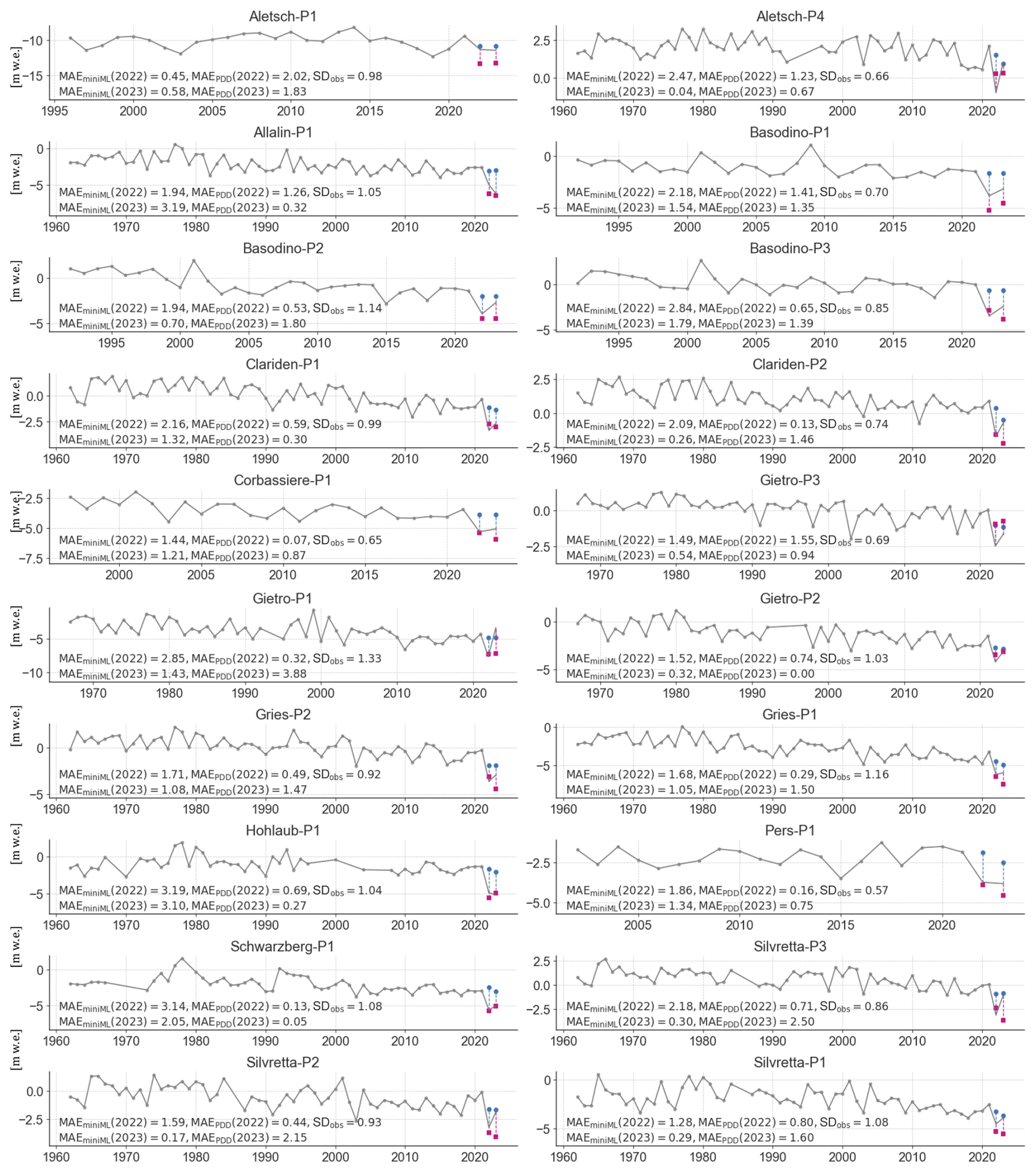
Figure A2 Predictions of extreme years (2022 and 2023) by miniML-MB (blue dots), trained within the optimal-seasonal framework, compared to the positive degree-day (PDD) baseline (pink square) for 28 sites on 13 glaciers. Both miniML-MB and the PDD model are trained with a time series that stops in 2021 and is tested based on 2022 and 2023. The mean absolute error (MAE) and root-mean-squared error (RMSE) are calculated between, respectively, the predictions of miniML-MB or the PDD model and the observed PMB (grey lines) over all test years.

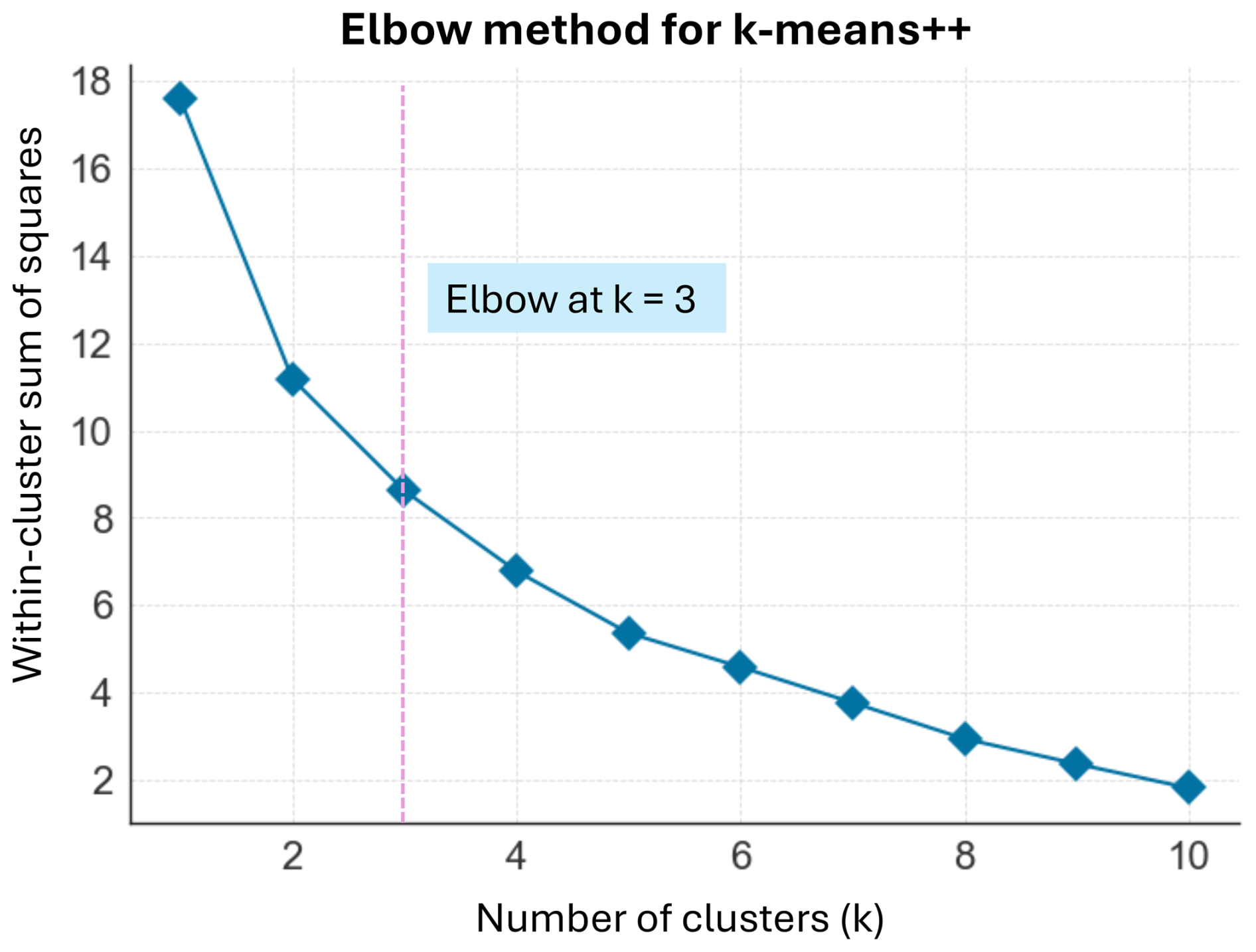
Figure A3 Optimal number of clusters of sites assigned using the k-means++ algorithm according to their drivers of point surface mass balance (see Sect. 5.6). For each number of clusters, the sum of squared distances from each site to its assigned centre is plotted, and the optimal number is the point of inflection on the curve (or “elbow”).

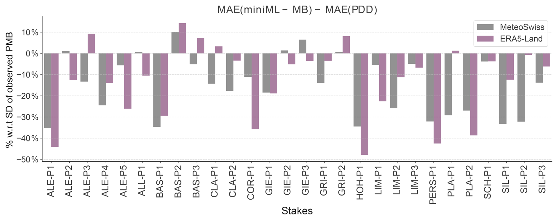
Figure A4 Comparison of the performance of miniML-MB, trained within the optimal-seasonal framework, when given MeteoSwiss (grey) or ERA5-Land (pink) input meteorological variables. The bars are the difference in mean absolute error (MAE) between miniML-MB and PDD models for all sites. The difference in MAE between both models is expressed in terms of percentage with respect to the standard deviation (SD) of the observed PMB. Bars above 0 signify that the PDD model is closer to the observed PMB, whereas bars below 0 indicate that miniML-MB is closer.

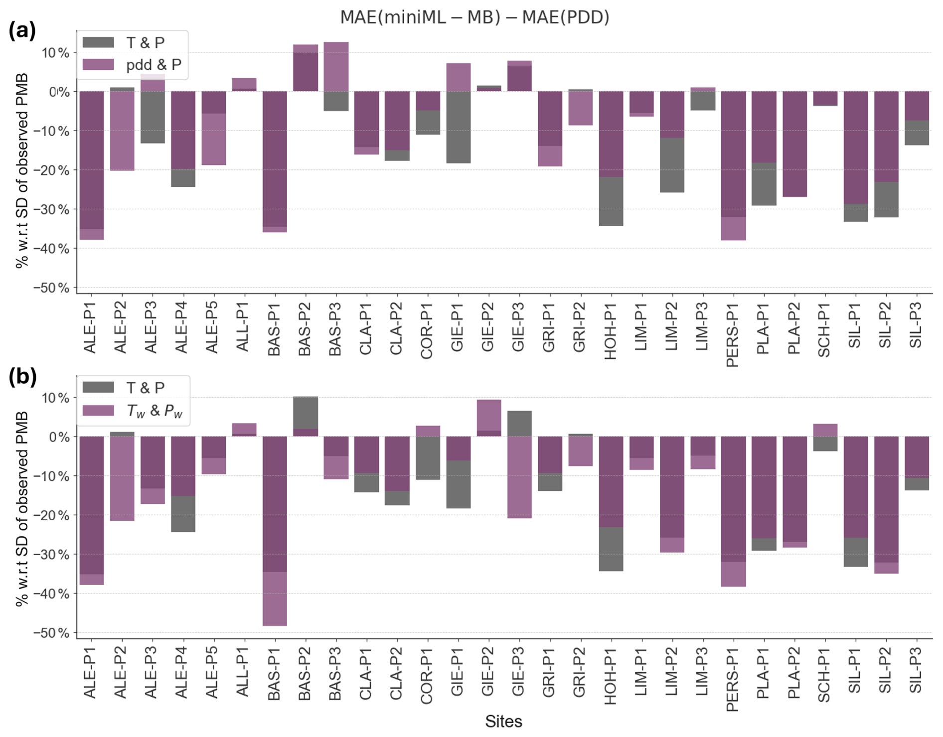
Figure A5 Comparison of the performance of miniML-MB when given different nuances of predictors based on air temperature (T) and total precipitation (P). (a) T and P (in grey) versus positive-degree-day temperatures (pdd) and P (in pink). (b) T and P (in grey) versus weighted T (T_w) and weighted P (P_w) (in pink). miniML-MB is trained within the optimal-seasonal framework using two predictors: mean T or pdd from May to August and P from October to February. The weights in (b) are [0.58, 1.0, 0.56, and 0.52] for T and [0.46, 0.6, 0.58, and 0.4] for P, i.e. the frequency of climate months in the 50 best combinations (Fig. 5). miniML-MB is compared to the positive-degree-day (PDD) baseline for all sites. The bars are the difference in the mean absolute error (MAE), expressed in terms of percentage with respect to the standard deviation (SD) of the observed PMB, between the miniML-MB and PDD models.