Thermal diffusivity of mountain permafrost derived from borehole temperature data in the Swiss Alps

Mountain permafrost is warming and thawing worldwide due to climate change, with ground temperature being a key control of its mechanical stability. Heat conduction is the dominant mode of heat transfer in frozen ground, and thermal diffusivity governs the rate at which temperature changes propagate through the subsurface. Despite its relevance, there are few field-based estimates of thermal diffusivity. In this study, we develop three mathematically independent formulations of the heat conduction equation to derive thermal diffusivity from borehole temperature data: (i) simple linear regression model (sLRM, statistical estimation), (ii) numerical inversion (semi-implicit finite-difference model), and (iii) analytical solution (explicit calculation). We first evaluate the validity of these three different approaches using a synthetically derived temperature dataset with known thermal diffusivities and then apply them to the 29 borehole temperature time series of the Swiss Permafrost Monitoring Network (PERMOS), enabling us to constrain thermal diffusivity in mountain permafrost with depth without prescribing any additional material properties. We obtain lumped thermal diffusivity values of the permafrost body for various permafrost landforms, with significant differences (median ± median absolute deviation): 1.5 ± 0.6 mm² s⁻¹ for bedrock, 1.1 ± 0.2 mm² s⁻¹ for talus slopes, and 1.3 ± 0.3 mm² s⁻¹ for ice bearing terrain like rock glaciers. This first compilation and analysis of empirically derived thermal properties of mountain permafrost advances the understanding of its thermal regime and provides key constraints for ground temperature and energy balance modeling. The application to real-world data further enables the identification of short-term non-conductive heat fluxes and the estimation of ground composition.

1 Introduction

Permafrost is defined in purely thermal terms, irrespective of water and/or ice content or lithological composition. It is a natural substrate that remains at or below 0 °C for at least two consecutive years (Muller, 1945). An overlying active layer, the uppermost few meters of seasonally frozen and thawed ground, forms the interface between the atmosphere and the permafrost. The thermal state of permafrost is a key indicator of climate change (IPCC, 2022) and permafrost is currently experiencing strong warming, shown by a measured increase in borehole temperatures in high-latitude regions (0.3 °C between 2007 and 2016, Biskaborn et al., 2019) and in European mountains (up to 1 °C between 2013 and 2022, Noetzli et al., 2024). The warming and thawing of permafrost can accelerate the release of large quantities of organic carbon currently stored in high-latitude regions of the Earth, thus accelerating climate change (Schuur et al., 2015; Strauss et al., 2024). In cold mountain areas, permafrost is spatially more variable and found in rock slopes at high elevations within various landforms, such as bedrock, talus slopes, and rock glaciers, where warming can reduce its mechanical stability, potentially leading to enhanced rock slope destabilization.

Overall, the thermal regime of the ground in mountain permafrost environments is governed by complex thermodynamic processes. While the dominant mechanism of heat transfer in the permafrost body (below the active layer) at depth is conduction (Haeberli et al., 2006), the thermodynamics of the overlying active layer are often characterized by additional, non-conductive heat fluxes (such as advection through water infiltration, vapor diffusion, and latent heat effects associated with phase changes; e.g., Hanson and Hoelzle, 2004; Scherler et al., 2014; Wicky and Hauck, 2017). The active heat exchange processes are strongly influenced by the site-specific physical properties of the rock, the ground composition – which can be a multiphase mixture of rocks of different sizes, ice, water, vapor, and air – as well as external factors such as the thickness of the snow cover, which not only provides insulation but also promotes water infiltration (Bonnaventure and Lamoureux, 2013). The thermal regime of the permafrost favors the replenishment of ice from water vapor in the near-surface and the formation and preservation of ground ice at depth once water is available (Taber, 1930; Murton and French, 1994). Exceptions occur when temperatures are close to 0 °C (Bast et al., 2024), when pressurized water flow takes place (Offer et al., 2024), or in the presence of fine-grained sediments (e.g., clay) or salt. In these latter cases, high unfrozen water contents may persist due to the freezing point depression of water (Williams, 1964).

Thermal diffusivity is a physical property that measures the ability of a material to conduct thermal energy relative to its ability to store thermal energy and thereby quantifies the rate of heat propagation in a material; in other words, it measures how quickly a material reacts to temperature changes. The physical property thermal diffusivity is thereby the one petrophysical parameter relevant in stationary and diffusive models without phase change of water (Yershov, 1998) as it controls the response of subsurface temperatures to surface forcing in a conductive regime and is, therefore, essential for understanding and predicting the dynamics of permafrost thermal regimes.

Despite the importance of thermal diffusivity, its values in permafrost are typically derived using literature values of the estimated thermal properties at the site or indirect model calibration (e.g. Magnin et al., 2017; Pruessner et al., 2021, 2022; Marcer et al., 2024) and often, in particular in mountain permafrost areas, these do not account for site-specific spatial variations in rock type, porosity, ice content, and moisture and related variations with depth. It remains challenging to validate estimates based on powerful models (e.g., CryoGrid; Westermann et al., 2023), which infer diffusivity by adjusting simulations to match temperature observations. In these cases, it is unclear whether the derived values reflect actual physical properties or compensate for other model uncertainties. Field-based estimations of thermal diffusivity remain scarce, particularly in high-mountain permafrost settings. Existing studies focus either on the active layer below the ground surface (for data from Matterhorn and Aiguille du Midi; Pogliotti et al., 2008) or the transition zone from the active layer to the top of the permafrost (in the high-alpine permafrost area Murtèl-Corvatsch; Schneider et al., 2012; Amschwand et al., 2025), without taking into account the underlying perennially frozen zone (permafrost body). Moreover, they rely on analytical solutions of the heat conduction equation, assuming idealized sinusoidal temperature variations during the investigated period without comparing the results with mathematically independent approaches. Consequently, there are no spatio-temporal (sub-annual) characterizations of thermal diffusivity for the underlying permafrost and no comparisons with independent approaches.

In this study, we aim to empirically estimate thermal diffusivity – i.e., the coefficient in the heat conduction equation – within the permafrost body below the active layer, by deriving it directly from in-situ borehole temperature observations in a purely data-driven manner without assumptions about material properties. We exploit existing borehole temperature records from the Alps using three approaches: (i) simple linear regression modeling (sLRM, statistical estimation), (ii) numerical inversion (semi-implicit finite-difference model), and (iii) analytical solution (explicit calculation) of the heat conduction equation. These approaches make use of the fact that thermal diffusivity not only integrates the three material properties thermal conductivity, specific heat capacity, and density but also links the temperature Laplacian and the temperature change rate (see Sect. 2.3). This relation forms the basis for our estimation of thermal diffusivity from borehole temperature time series at different depths and over time, as it allows us to determine thermal diffusivity without the assumption of any material properties. With these three mathematically independent methods, the systematic analysis of the Swiss Permafrost Monitoring Network borehole temperature data (PERMOS, 2024) allows us to derive a representative range for the thermal diffusivity values in mountain permafrost under natural conditions with examples from bedrock, talus slopes, and ice-rich rock glaciers.

While in-situ temperature data capture site-specific variations and provide a realistic representation of heat transfer processes, the direct estimation of thermal diffusivity from borehole temperature time series is crucial for improving thermal modeling and for applied permafrost studies. In addition, to reduce simulation uncertainties in permafrost models and enhance the reliability of ground temperature predictions, these thermal diffusivity values, for example, also permit (i) the extraction of ground composition through the comparison of observed values with established thermal properties of distinct materials or (ii) the isolation of short-term non-conductive heat fluxes by identifying thermal anomalies.

2 Data and methods

In this study, we use two types of borehole temperature time series. First, synthetic permafrost data are used to develop and validate our approaches for inferring thermal diffusivity. Second, we apply these methods to mountain permafrost borehole data to empirically estimate thermal diffusivity within the permafrost body below the active layer, where thermal conduction dominates the temperature evolution.

2.1 Synthetic permafrost borehole temperatures

We analytically generate two synthetic permafrost borehole temperature time series using predefined thermal diffusivity values (1 and 5 mm² s⁻¹) to validate and assess the performance of the three developed approaches (see Sect. 2.3). We evaluated different temperature sensor spacings and temporal window sizes. We simulate an exemplary temperature regime of a permafrost body with the characteristics of the borehole COR_0315 drilled in 2015 on rock glacier Murtèl-Corvatsch by applying a geothermal heat flux of 50 mW m⁻² for initial temperature distribution down to 17 m depth and a sinusoidal surface temperature forcing with a mean annual ground surface temperature (MAGST) of −2.5 °C and an annual amplitude of 10 °C. This produces temperature variations that are typical of the permafrost body below the active layer depth (for details, see Appendix B and Fig. B1).

2.2 Mountain permafrost borehole temperatures

We analyze 29 measured PERMOS borehole temperature time series (PERMOS, 2024) to infer thermal diffusivities in mountain permafrost across the Swiss Alps. These boreholes, ranging from 14 to 100 m in depth, are distributed across 15 sites (Fig. 1a) encompassing the landforms bedrock, talus slopes, and rock glaciers (see Fig. 1b). Detailed borehole descriptions are provided in PERMOS (2019). This study uses cleaned, daily aggregated data from the start of measurements until 1 June 2023 (PERMOS, 2024), resulting in time series ranging from 4 to 36 years. Since the Murtèl-Corvatsch rock glacier is extensively monitored and has been the focus of numerous studies (e.g., Arenson et al., 2010; Schneider et al., 2012; Scherler et al., 2014; Marmy et al., 2016; Cicoira et al., 2019; Pruessner et al., 2021, 2022; Amschwand et al., 2024, 2025), we use the borehole COR_0315 drilled in 2015 on rock glacier Murtèl-Corvatsch as an illustrative example throughout this study. The evolution of the thermal regime over time and with depth is illustrated in Fig. 1c–e.

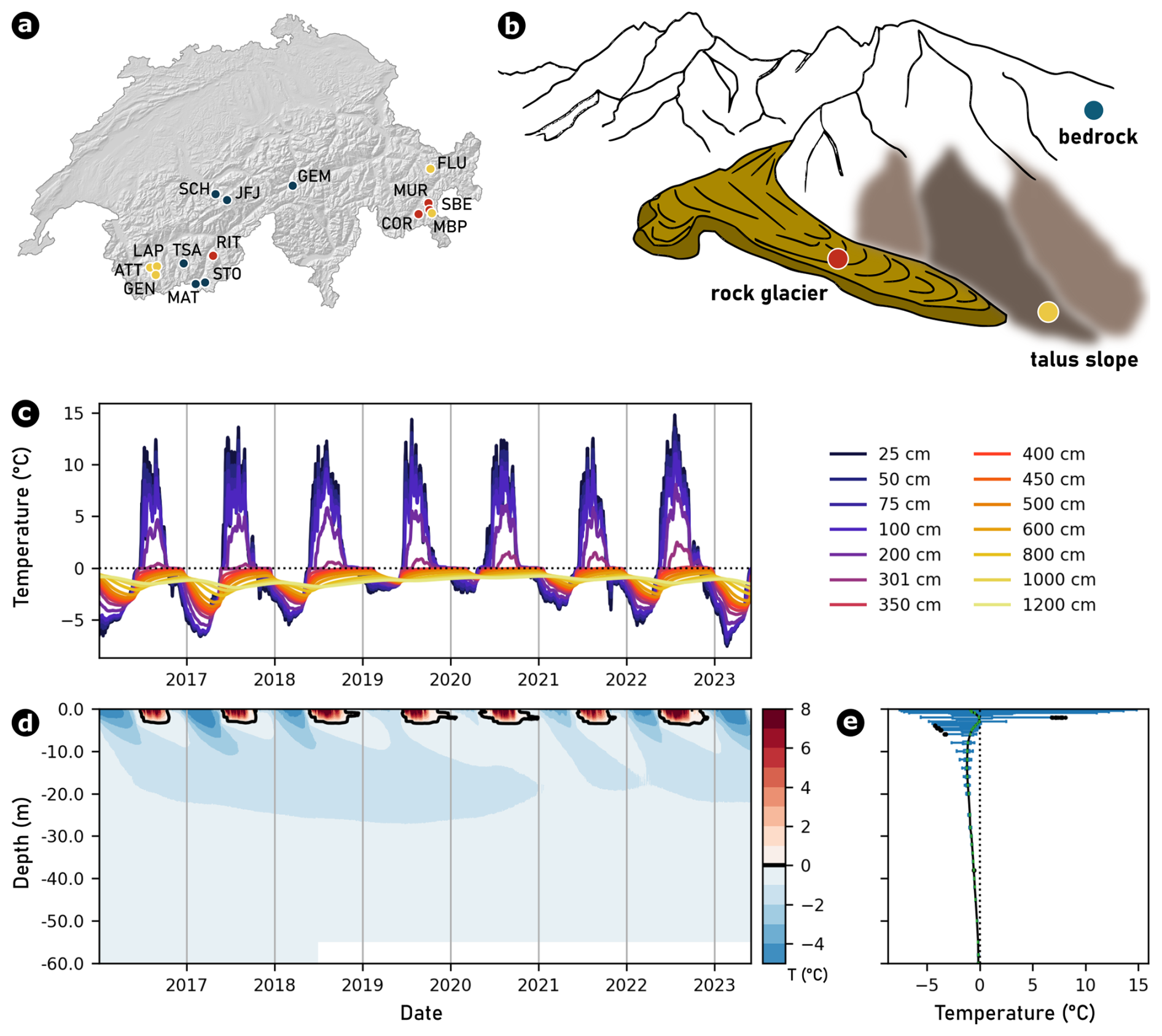
Figure 1 (a) Map of Switzerland providing an overview of the 15 PERMOS field sites with three-character abbreviations (explanation in Swiss Permafrost Bulletin 2023; PERMOS, 2024) and colors referring to the type of landform as shown in (b) a schematic visualization of three typical mountain permafrost landforms: bedrock, talus slope, and rock glacier. As an illustrative example, (c) temperature time series for selected depths, (d) a temperature contour plot for the entire depth, and (e) mean temperature profiles of borehole COR_0315 on Murtèl-Corvatsch are shown.

2.3 Quantifying thermal diffusivity

The general form of energy conservation states that the rate of change of heat energy within a control volume equals the net heat flux into the volume, including both conductive (q_c in W m⁻²) and non-conductive (q_nc in W m⁻²) heat fluxes, as well as any internal heat sources or sinks (S in W m⁻³) over time (Bergman et al., 2020)

$$\begin{array}{}\text{(1)}& \partial Q/\partial t=-\mathrm{\nabla }\cdot ({\mathbf{q}}_{\mathrm{c}}+{\mathbf{q}}_{\mathrm{nc}})+S,\end{array}$$

where Q is the internal heat energy per unit volume (in J m⁻³) and t is time (in s). Assuming no significant heat sources (S=0) and neglecting non-conductive heat fluxes (q_nc=0), which mostly applies below the active layer, the energy conservation equation simplifies to

$$\begin{array}{}\text{(2)}& \partial Q/\partial t=-\mathrm{\nabla }\cdot {\mathbf{q}}_{\mathrm{c}}.\end{array}$$

The heat conservation equation states that the rate of change of heat content is equal to the net heat flux divergence

$$\begin{array}{}\text{(3)}& \partial Q/\partial t=C\cdot \partial T/\partial t,\end{array}$$

where C=ρc_p is the volumetric heat capacity, combining the material density (ρ) and specific heat capacity (c_p). This term quantifies the amount of energy required to raise the temperature of a unit volume by one kelvin. Substituting Fourier's law, which states that conductive heat flux is proportional to the temperature gradient (${\mathbf{q}}_{\mathrm{c}}=-k\mathrm{\nabla }T$), into the energy conservation equation (Fourier, 1822)

$$\begin{array}{}\text{(4)}& C\cdot \partial T/\partial t=\mathrm{\nabla }\cdot \left(k\mathrm{\nabla }T\right),\end{array}$$

describes the energy transfer through a solid medium with a temperature gradient over time and in space with variations in temperature T (in °C) and the thermal conductivity k (in W m⁻¹ K⁻¹) governing how temperature variations propagate through the ground. Rearranging the equation by expressing thermal conductivity k with thermal diffusivity $\mathit{\kappa }=k/C$ and treating κ(z) as piecewise constant with depth – allowing for different but uniform diffusivity values within distinct subsurface layers to better represent heterogeneity – yields

$$\begin{array}{}\text{(5)}& \partial T/\partial t=\underset{\begin{array}{c}\text{neglected by treating}\mathit{\kappa }\text{as}\\ \text{piecewise constant with depth}\end{array}}{\underbrace{\mathrm{1}/C\cdot \mathrm{\nabla }(\mathit{\kappa }\cdot C)\cdot \mathrm{\nabla }T}}+\mathit{\kappa }\cdot {\mathrm{\nabla }}^{\mathrm{2}}T,\end{array}$$

with ∇² the Laplace operator (in m⁻²). Thermal diffusivity is thus a thermal property that determines how efficiently heat propagates through the ground relative to its ability to store thermal energy. An overview of the thermal properties of water, ice and air, and different rock types and minerals is given in Table 1, highlighting the strong variability and spread that occurs in nature. Assuming that diffusivity is constant in space within each set of three consecutive temperature sensors along the profile and that heat flows by conduction only in the vertical direction (i.e., perpendicular to the ground surface), the use of the simplified heat conduction equation in the differential form (Carslaw and Jaeger, 1959)

$$\begin{array}{}\text{(6)}& \partial T/\partial t=\mathit{\kappa }{\partial }^{\mathrm{2}}T/\partial z^{\mathrm{2}},\end{array}$$

allows for determining thermal diffusivity based on borehole temperature time series at different depths and over time without knowledge of material properties. For this, we designed a suite of empirical models to quantify thermal diffusivity κ in mountain permafrost solely through heat conduction, implementing these approaches in Python 3 (Weber et al., 2025b). Convective/advective heat flows and phase changes are not included in this equation and therefore not considered in the proposed modeling approaches. Our modeling inferences therefore focus mostly on the permafrost body below the active layer. Using temperature profile time series from boreholes, we perform statistical analyses (simple Linear Regression Model, for example applied to supraglacial debris by Nicholson and Benn, 2013) to infer thermal diffusivity (coefficient of the heat conduction equation Eq. 6) and compare the results obtained with numerical inversion (Crank-Nicolson semi-implicit finite-difference method, for example applied to rock glaciers by Cicoira et al., 2019) and analytical solution (for example applied to bedrock and rock glaciers, Pogliotti et al., 2008; Schneider et al., 2012). In each modeling approach, iterating along the profiles, we consider three equally spaced adjacent temperature sensors and assign the derived thermal diffusivity values to the middle one; this is done for given window sizes (see Sect. 3.2 for details) and with a time-stepping of 7 d.

Table 1 The essential thermal properties of selected end-range elements, rock types, and minerals. (References: Blackwell and Steele, 1989; Clauser and Huenges, 1995; Waples and Waples, 2004; Haigh, 2012; Labus and Labus, 2018; Jia et al., 2019)

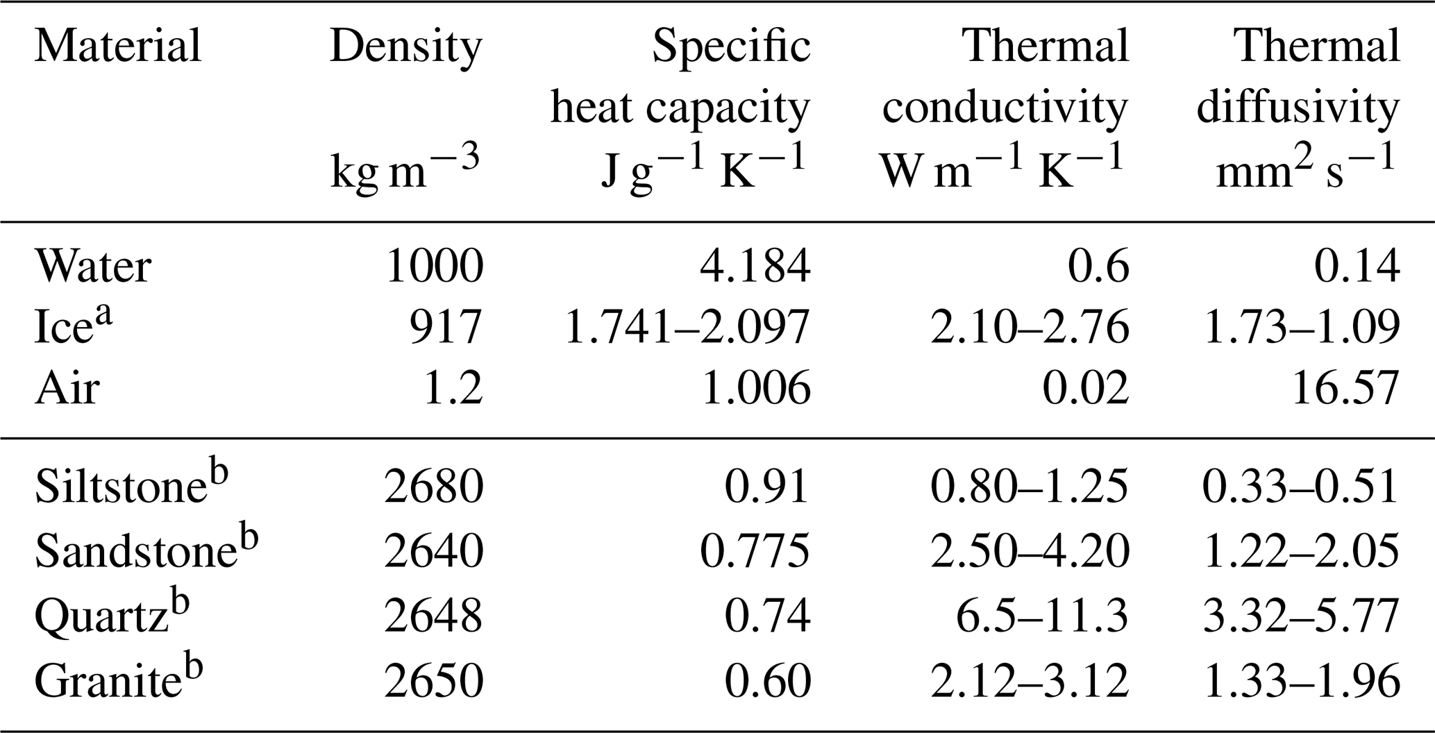
^a The values for the specific heat capacity as well as the thermal conductivity of ice are temperature-dependent and specified for temperatures at −50 and 0 °C, respectively. ^b The specific heat capacity and the thermal conductivity are both sensitive to density and moisture content.

sLRM analysis.

For the statistical analysis, we followed the approach outlined by Nicholson and Benn (2013), incorporating parts of the analysis code from Petersen (2022) – both studies with application to supraglacial rock debris. Using sets of three equally spaced sensors along the borehole profile, we first applied different numerical techniques to the discrete depth and temperature values to compute the first and second derivatives along the profile for each sensor: the first derivative of temperature with respect to time at the middle sensor $\partial T/\partial z$ using the central difference based on the depths of the neighboring sensors and taking into account the actual distances, and the second derivative of temperature with respect to depth between the upper and lower sensors ${\partial }^{\mathrm{2}}T/\partial z^{\mathrm{2}}$ by their finite differences (for details of the calculation, see Appendix A). We then performed a simple Linear Regression Model (sLRM) analysis that relates the temperature Laplacian (${\partial }^{\mathrm{2}}T/\partial z^{\mathrm{2}}$) to the temperature change rate ($\partial T/\partial t$) to estimate the thermal diffusivity (κ, the heat conduction coefficient in Eq. 6) for the depth corresponding to the middle sensor. This relation allows us to estimate the thermal diffusivity from the temperature profiles measured at each sensor location. Considering the multiple linear regression model (mLRM) approach of Petersen et al. (2022), which is based on the one-dimensional heat conservation equation for the near-surface layer of debris-covered glaciers, accounts for depth-dependent variations in thermal diffusivity modulated by the temperature gradient

$$\begin{array}{}\text{(7)}& \partial T/\partial t=\underset{\begin{array}{c}\text{considered by}\\ \text{Petersen et al.}\\ \text{(2022)}\end{array}}{\underbrace{\partial \mathit{\kappa }/\partial z\cdot \partial T/\partial z}}+\mathit{\kappa }{\partial }^{\mathrm{2}}T/\partial z^{\mathrm{2}}.\end{array}$$

To simplify Eq. (7), we assume a homogeneous bulk material within the vertical segment defined by a set of three consecutive sensors along the borehole and therefore treat the first derivative of κ with respect to depth as piecewise constant within each segment ($\partial \mathit{\kappa }/\partial z=\mathrm{0}$). This still enables the derivation of a depth-dependent thermal diffusivity profile κ(z) along the entire borehole, thereby better representing vertical heterogeneity in subsurface thermal properties. This decision is also justified on methodological grounds as there is a strong correlation between the variables $\partial T/\partial z$ and ${\partial }^{\mathrm{2}}T/\partial z^{\mathrm{2}}$, which makes them unsuitable for mLRM analysis. In comparison to Nicholson and Benn (2013) and Petersen et al. (2022), we ensure that the following regression assumptions are met: (1) no multicollinearity, (2) independence of errors, (3) normally distributed residual errors, and (4) homoscedasticity. These assumptions are assessed by diagnostic plots (see Fig. C1). We then only consider valid regression models with a significance level of p<0.01 and a coefficient of determination R²>0.7 for further analysis.

Numerical inversion.

For the numerical solution of the heat equation, we applied the Crank-Nicolson approach, a semi-implicit finite-difference scheme that combines the explicit (forward-time centered-space) and implicit (backward-time centered-space) formulations (Crank and Nicolson, 1947). While balancing computational efficiency and numerical precision, this method ensures stability and maintains second-order accuracy in both time and space, making it particularly suitable for heat diffusion problems in ice sheet, alpine glacier, and permafrost studies (e.g., Dahl-Jensen et al., 1999; Wilson and Flowers, 2013; Carenzo et al., 2016; Cicoira et al., 2019,  respectively). The one-dimensional heat equation is discretized as

$$\begin{array}{}\text{(8)}& \begin{array}{rl}{\displaystyle \frac{T_i^{n+\mathrm{1}}-T_i^n}{\mathrm{\Delta }t}}& ={\displaystyle \frac{\mathit{\kappa }}{\mathrm{2}\mathrm{\Delta }{z}^{\mathrm{2}}}}\left[\left(T_{i+\mathrm{1}}^{n+\mathrm{1}}-\mathrm{2}{T}_i^{n+\mathrm{1}}\right.\right.\\ & \left.\left.+T_{i-\mathrm{1}}^{n+\mathrm{1}}\right)+\left(T_{i+\mathrm{1}}^n-\mathrm{2}{T}_i^n+T_{i-\mathrm{1}}^n\right)\right].\end{array}\end{array}$$

where $T_i^n$ represents the temperature at spatial index i and time step n, κ is the thermal diffusivity, and Δt and Δz are the constant differences in time window and in depth step sizes, respectively. This formulation leads to a tridiagonal system of equations that must be solved at each time step, allowing for larger time steps than explicit schemes without sacrificing numerical stability. By iteratively solving for Tⁿ⁺¹, the method efficiently models subsurface temperature evolution while minimizing numerical diffusion. For each set of three consecutive sensors along the profile and each time window, we performed this numerical solution 101 times using different values of κ ranging from 0–10 mm² s⁻¹ with a step of 0.1 mm² s⁻¹ to model the temperature at the central sensor using the temperature measurement time series of the lower and upper sensors. The initial condition was prescribed from the measured vertical temperature profile at the first time step of the simulation within the given time window. The temporal resolution of the model, determined by the temporal resolution of the temperature time series, is 1 d, and the vertical resolution depends on the sensor spacing but is limited to a minimum of 0.01 m. We then solved a minimum problem by iteratively approaching the most representative value for thermal diffusivity by minimizing the RMSE (Root Mean Square Error) between the modeled and observed temperature time series at the middle sensor within the given time window.

Analytical solution.

For the analytical solution of the heat conduction equation and the explicit calculation of the thermal diffusivity, the one-dimensional heat conduction equation (Eq. 6) can be solved at any depth z using a harmonic temperature boundary condition at the surface (Williams and Smith, 1991):

$$\begin{array}{}\text{(9)}& T(z,t)={\stackrel{\mathrm{‾}}{T}}_z+A_{\mathrm{s}}{e}^{-z(\mathit{\omega }/\mathrm{2}\mathit{\kappa }{)}^{\mathrm{1}/\mathrm{2}}}\sin \left[\mathit{\omega }t-{\left(\mathit{\omega }/\mathrm{2}\mathit{\kappa }\right)}^{\mathrm{1}/\mathrm{2}}z\right],\end{array}$$

where A_s is the amplitude of the surface temperature wave, $\mathit{\omega }=\mathrm{2}\mathit{\pi }/P$ with the period P of the temperature oscillation (e.g., daily or annual cycle), and ${\stackrel{\mathrm{‾}}{T}}_z$ the baseline temperature at depth z around which the periodic variations (caused by the sinusoidal term) occur. Time t is counted from the date when the surface temperature wave passes through its mean value within the oscillation period. Using the amplitudes A₁ and A₂ of the temperature waves (°C) at the depths z₁ and z₂ (m) of the upper and lower sensors from each set of three consecutive sensors along the borehole profile, we then invert the thermal diffusivity κ at the middle sensor (Horton et al., 1983; Matsuoka, 1994)

$$\begin{array}{}\text{(10)}& \mathit{\kappa }=\mathit{\pi }/P{\left[{\displaystyle \frac{z_{\mathrm{2}}-z_{\mathrm{1}}}{\ln \left(A_{\mathrm{1}}/A_{\mathrm{2}}\right)}}\right]}^{\mathrm{2}}.\end{array}$$

This method provides a bulk estimate of thermal diffusivity for the subsurface from observed borehole temperature time series and has been applied in other permafrost studies (e.g., Pogliotti et al., 2008; Schneider et al., 2012). However, it relies on several key assumptions: (i) heat transfer is dominated by conduction, (ii) temperature variations at any depth follow a purely sinusoidal cycle without irregular fluctuations, and (iii) a steady-state condition, where the long-term temperature distribution at depth remains stable without significant trends over time. In practice, however, variations in ground composition, non-periodic temperature changes, and measurement uncertainties can introduce deviations from the idealized assumptions, requiring careful evaluation of the method's applicability to specific field conditions.

Examples of the performance and representativeness of the derived thermal diffusivity obtained by applying the sLRM and numerical inversion to the case of Murtèl-Corvatsch are shown for a depth of 10 m and within the 3-month time window from 22 April to 22 July 2016 (see Fig. 2). The sLRM fulfills all assumptions in this time window (see diagnostic plots in Fig. C1) and provides an estimated thermal diffusivity of 1.31 mm² s⁻¹ with a high coefficient of determination (R²=0.80) as well as a low p-value (<0.001; Fig. 2a). A direct comparison between the observations on the horizontal axis with the sLRM prediction output on the vertical axis also highlights a significant correlation (p<0.001; Fig. 2b). The numerical solution provides a slightly higher diffusivity value of 1.5 mm² s⁻¹ (yellow line in Fig. 2c) with a highly significant representativeness (Fig. 2d). Both approaches perform under purely conductive conditions but fail during periods characterized by phase change (e.g., during the spring and autumn zero curtains in the active layer) or when non-conductive heat fluxes occur due to, for example, water fluxes (see Fig. C2). Hence, we focus our analysis on depths below the active layer and omit estimated diffusivity values above.

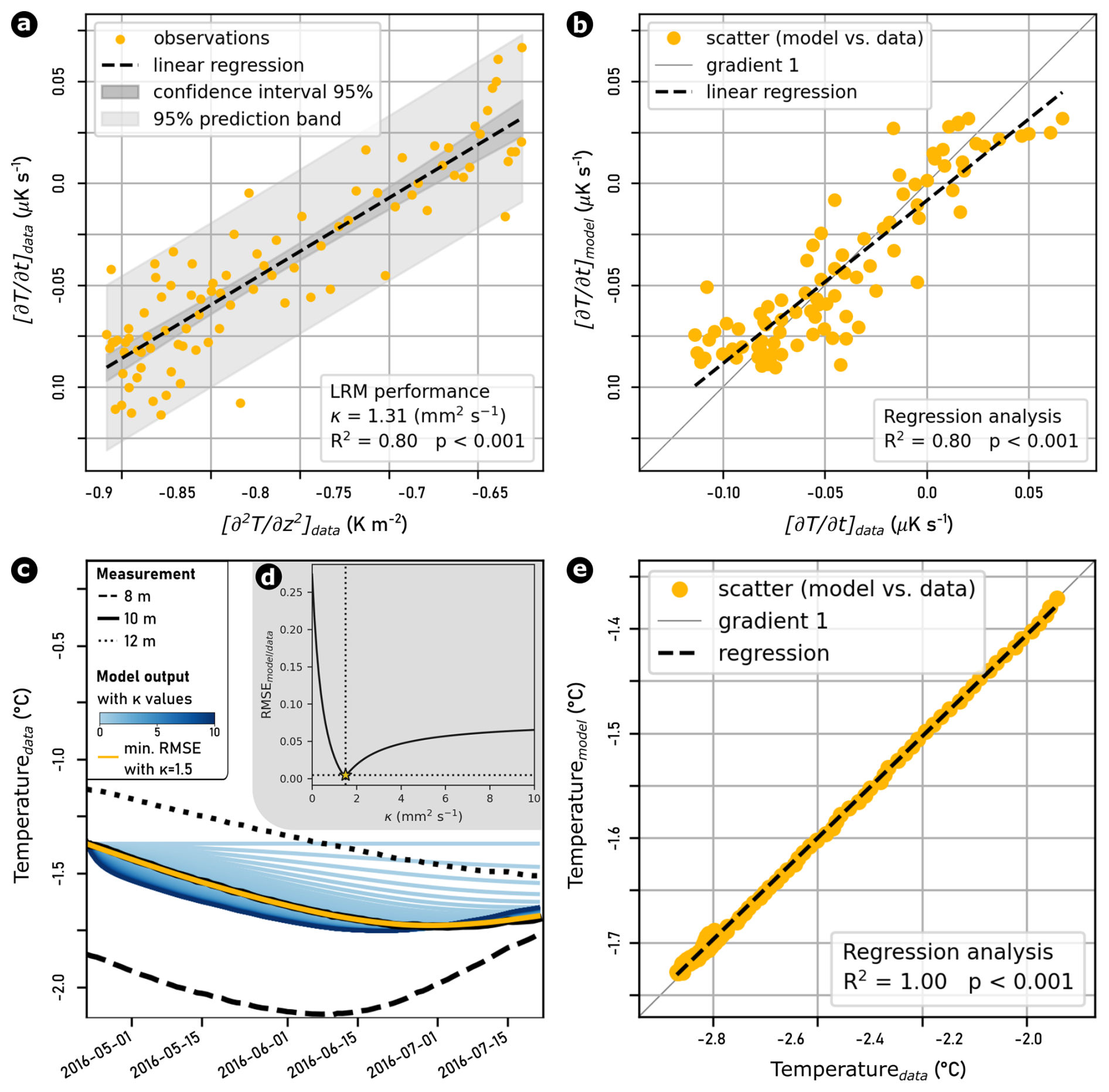
Figure 2 Empirically derived thermal diffusivity in the COR_0315 borehole on the Murtèl-Corvatsch rock glacier. Performance and representativeness of the sLRM (a, b) and the numerical inversion (c, e) at 10 m depth and in the 3-month time window from 22 April to 22 July 2016. (d) Iterative approximation to the most representative value for the thermal diffusivity by minimizing the RMSE (Root Mean Square Error) between the modeled and the observed temperature time series.

All three thermal diffusivity estimation approaches rely on different assumptions, influencing the appropriate choice of time window size for analysis. To evaluate the performance and sensitivity of the three modeling approaches, we first conducted a synthetic experiment using multiple temperature time series generated with known thermal diffusivities (see Sect. 3.1). This allowed us to assess how accurately each method could recover the predefined diffusivity values under varying window sizes and configurations. We then applied the same approaches to field temperature data from the mountain permafrost borehole COR_0315 as an illustrative example, enabling a quantitative intercomparison of the methods in terms of temporal consistency and coverage of derived thermal diffusivity values (see Sect. 3.2). Based on these results, we determined appropriate time window sizes for each approach. For the analytical solution approach, we restrict the analysis to 12-month windows that fully capture both the seasonal temperature signal at the upper sensor and its delayed response at the lower one to ensure the validity of the periodic forcing assumption, as at least one complete temperature cycle is necessary and allows for a consistent and reliable estimation of thermal diffusivity. After the investigation of variation of thermal diffusivity with depth for borehole COR_0315 on Murtèl-Corvatsch (see Sect. 3.3), we applied selected approaches using 12-month windows to each set of three adjacent sensors with depth for all PERMOS boreholes to derive thermal diffusivity in the mountain permafrost body for various landforms (see Sect. 3.4).

3 Results and Interpretation

3.1 Synthetic experiment evaluating methods and sensitivities to time window size

The performance of the statistical and numerical approaches was assessed using a synthetic dataset with predefined thermal diffusivity values for different window sizes and sensor spacings (see Fig. 3). For equally spaced sensor sets (Fig. 3a), the statistical and numerical approaches yield median values consistent with the known thermal diffusivity values across all time window sizes and depths. However, the sLRM shows increased scatter with decreasing time window size for all depths. In contrast, the numerical inversion only exhibits this behavior at the greatest depth, likely due to decreasing temperature change rates and gradients. For non-uniform sensor spacing (e.g., set of three consecutive sensors at 5.5, 6 and 7 m depths; Fig. 3b), the numerical inversion performs well except for short time window sizes (1 and 3 months), when the temperature change rates and gradients decrease at greater depths. The statistical approach, on the other hand, consistently deviates from the target values across all window sizes and depths, with the offset increasing as the window size decreases and depth increases. Consequently, we restrict our successive analysis of unequally spaced sensor sets to numerically and analytically derived diffusivity values for 12-month windows, excluding shorter window sizes and the statistical approach altogether.

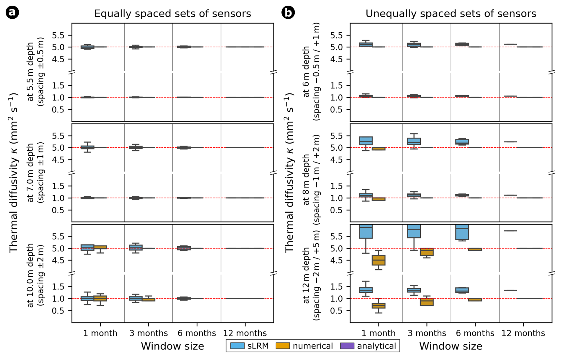
Figure 3 The performance of all three modeling approaches applied to the synthetic dataset with predefined thermal diffusivity values (1 and 5 mm² s⁻¹, indicated by red horizontal lines), evaluated for different time window sizes (1, 3, 6, and 12 months; analytical solution shown only for 12-month windows) and sensor spacings. Each boxplot represents n>30 different time steps. Panel (a) shows results for equally spaced temperature sensors, while panel (b) presents results for unequally spaced sensor configurations.

3.2 Selection of appropriate temporal window size

While this performance assessment with the synthetic data set has stable boundary conditions, field borehole temperature records in mountain permafrost often exhibit long-term warming (e.g., Noetzli et al., 2024), non-linear phase change effects (e.g., latent heat exchange in permafrost) or non-conductive heat flow. When applying our approaches to the case of Murtèl-Corvatsch, depending on the length of the analyzed window size, we observe temporal variations in thermal diffusivity (see Fig. 4). A direct comparison of the inferred thermal diffusivities through sLRM and numerical inversion within 3-month windows at 10 m depth show comparable mean values with a normally distributed scattering (see Fig. C3).

The simple linear regression model (sLRM) for estimating thermal diffusivity assumes a linear relation between temperature changes at different depths over time, as expected under purely conductive heat transfer in a homogeneous medium. This assumption holds best when the temperature signal evolves gradually and consistently, such as during periods of slow, steady warming or cooling. This assumption breaks down if the temperature signal includes trend reversals, such as a transition from warming to cooling, which violates the model's expectation of a consistent thermal gradient over time and can lead to a distortion of the inferred thermal diffusivity values (see Fig. 4b). Therefore, applying sLRM over longer time windows (e.g., six months or one year) introduces errors because the ground temperature response to surface forcing is inherently non-linear over such timescales. Specifically, longer windows encompass the full annual cycle of temperature fluctuations, including seasonal extremes and transitions, which cause curvature in the temperature–time profiles at different depths due to damping and phase shifts with depth. This non-linearity violates the core assumption of sLRM, leading to biased regression results and inaccurate diffusivity estimates. When sLRM is applied to shorter time windows, the temperature evolution at a given depth can be approximated as linear, especially during periods with nearly constant or slowly changing surface forcing. In these cases, the vertical propagation of the thermal signal follows a more consistent gradient, making the linear regression between temperature time series at adjacent depths more reliable. Consequently, the derived thermal diffusivity primarily reflects the conductive behavior of the material and is less influenced by transient or cumulative non-linear effects. This results in an effective thermal diffusivity that better represents the material properties under those specific, quasi-steady thermal conditions. Note that non-conductive effects are automatically omitted as the assumption for the sLRM fails (see Fig. C2).

In contrast, numerical inversion of the heat conduction equation to derive thermal diffusivity – by iteratively adjusting diffusivity to minimize the root mean square error (RMSE) between modeled and measured temperature profiles – tends to become more robust when applied over longer time windows (e.g., six months to one year). This is because longer periods capture a broader portion of the periodic surface temperature signal and its propagation into the subsurface, particularly the annual cycle, which dominates temperature variability at depth. As a result, short-term fluctuations and high-frequency noise are averaged out, yielding a more stable estimate of thermal diffusivity. This broader temporal integration allows the inversion approach to better resolve the cumulative effects of heat transfer dynamics and to smooth out localized anomalies that may distort shorter time window results. Moreover, longer time windows help constrain the thermal diffusivity that governs the full amplitude and phase shift of the seasonal signal across depths, which is essential for capturing the bulk behavior of the subsurface thermal regime. However, this comes at the cost of reduced sensitivity to transient features and introduces potential bias if the longer time period includes processes that deviate from purely conductive behavior – such as latent heat effects, water fluxes, or variable surface forcing. These influences, though averaged out to some extent, may still be embedded in the resulting estimate and contribute to a so-called “apparent” thermal diffusivity that refers to the empirically derived thermal diffusivity integrating site-specific heterogeneity effects. Thus, while numerical inversion over long time windows can yield a more globally consistent and robust diffusivity value for modeling purposes, careful interpretation is needed to separate the effects of physical material properties from those of process-induced variability.

For the analytical solution, which is based on matching measured temperature profiles to the mathematical form of a damped and phase-shifted sinusoidal wave, a full seasonal period is essential to properly resolve the subsurface temperature signal (for details, see Sect. 2.3). This is because the method assumes a steady periodic boundary condition (typically annual) and relies on the amplitude decay and phase lag of the thermal wave with depth to estimate thermal diffusivity. Applying the analytical solution over shorter time windows that do not span at least one full seasonal cycle would violate this assumption and lead to unstable or biased diffusivity estimates due to incomplete wave resolution. Using long time windows – ideally one year or more – not only ensures consistency with the assumptions of the analytical solution but also enhances the signal-to-noise ratio, as short-term variability, asymmetry in temperature evolution, and transient influences are smoothed out. This allows the extracted thermal diffusivity to reflect the material’s ability to transmit the dominant periodic (seasonal) signal. However, similar to the inversion approach, the analytical solution over longer windows may also integrate the effects of non-conductive processes or temporal changes in surface forcing, which can alter wave characteristics. As a result, the derived diffusivity represents an apparent value, encapsulating both intrinsic material properties and the influence of longer-term thermal dynamics. Considerably lower thermal diffusivity values from summer 2018 to 2020 are attributed to the multi-year particularly warm period characterized by a sustained warming trend (see Fig. 4d). Therefore, careful consideration is needed when interpreting such values, especially in heterogeneous substrates or hydrologically active permafrost environments.

For the subsequent spatio-temporal analysis of all PERMOS borehole temperature records, we therefore focus on the numerical and analytical approaches using 12-month time windows, as shorter (sub-annual) windows are more susceptible to data gaps that compromise the statistical robustness of the analysis. A potential application of the sLRM method in permafrost research is discussed separately in the discussion section (see Sect. 4.2).

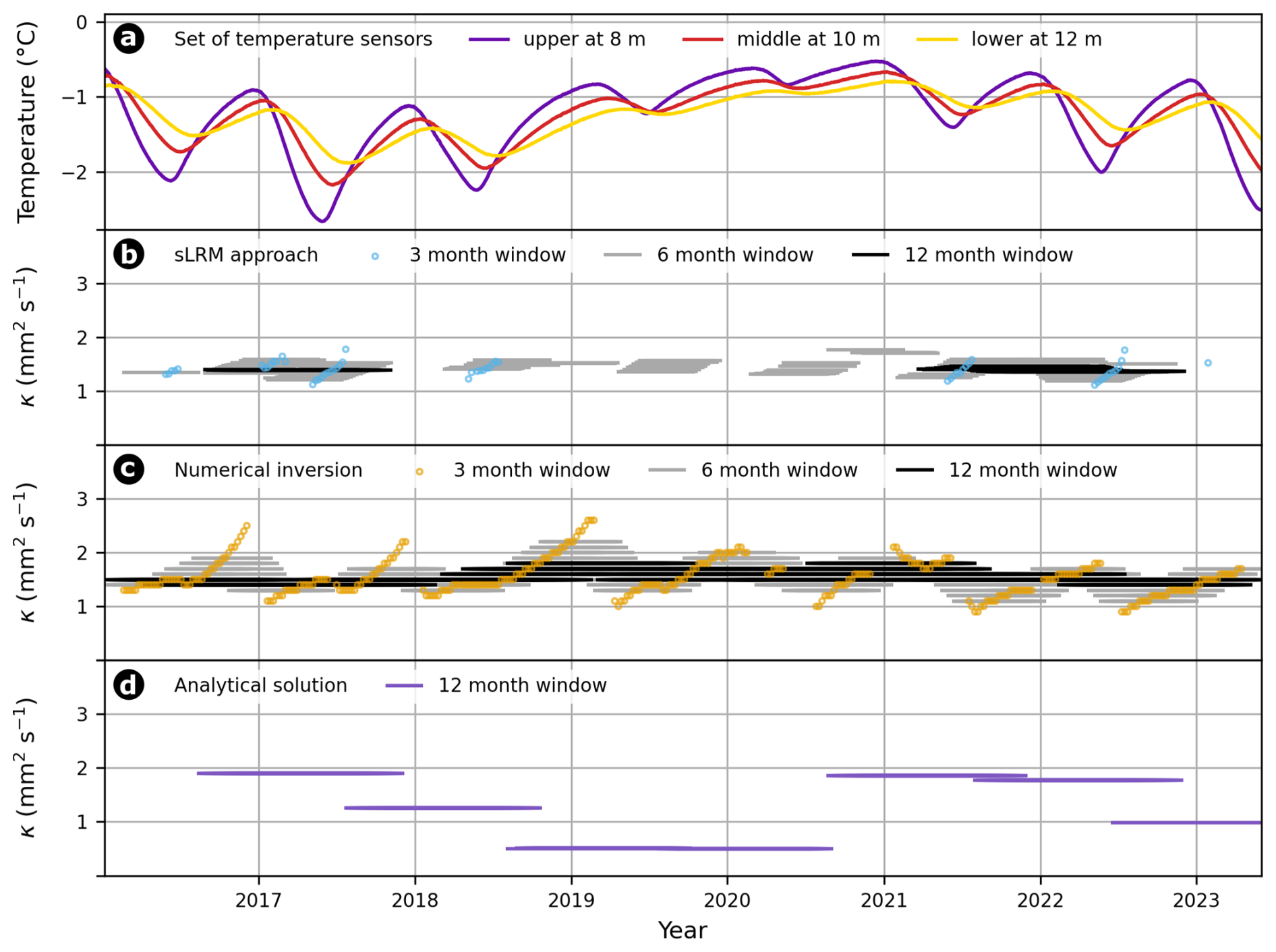
Figure 4 The multi-year time series of borehole temperature (a) and thermal diffusivity derived through (b) linear regression analysis of the heat conduction equation, (c) numerical inversions and (d) analytical solutions for borehole COR_0315 on Murtèl-Corvatsch at 10 m depth. For both the statistical and numerical approaches, different window sizes were tested and compared, revealing approach-dependent differences in performance. For the subsequent spatio-temporal analysis, we focus on the numerical and analytical methods using 12-month windows, as shorter (sub-annual) windows are more susceptible to data gaps that compromise result quality. A potential application of the sLRM approach in permafrost research is addressed in the Discussion.

3.3 Depth variation of apparent thermal diffusivity

The depth profile of apparent thermal diffusivity derived using both numerical and analytical approaches with 12-month windows is shown for borehole COR_0315 on Murtèl-Corvatsch in Fig. 5. Numerically derived values exhibit considerable variability within the active layer, whereas the analytical solution was only applied below the maximum active layer depth to ensure that the phase relation between the upper and lower thermistors in a sensor set is preserved. Within the permafrost body, i.e. below the active layer, thermal diffusivity estimates are more stable with depth and show good agreement between both approaches with overlapping median absolute deviations, although the analytically derived medians are slightly higher. At greater depths (not shown in Fig. 5), modeling becomes unreliable or statistically insignificant due to diminished annual temperature amplitudes approaching the level of measurement uncertainty (see Discussion). While analytical modeling performs well in the upper permafrost, uncertainty increases at 25 m depth with a significant deviation from the numerical output.

The large statistical variance observed in the active layer is attributed to seasonal variability in thermal diffusivity and the presence of non-conductive heat fluxes, such as advective heat transport from percolating water and latent heat exchange. The growing mismatch between methods with depth is explained by the decreasing annual temperature variation amplitude and the reduced number of time windows with valid diffusivity constraints. Consequently, for the subsequent statistical analysis, we focus exclusively on the permafrost body, where both numerical and analytical methods yield constrained values and phase change effects near 0 °C are minimized.

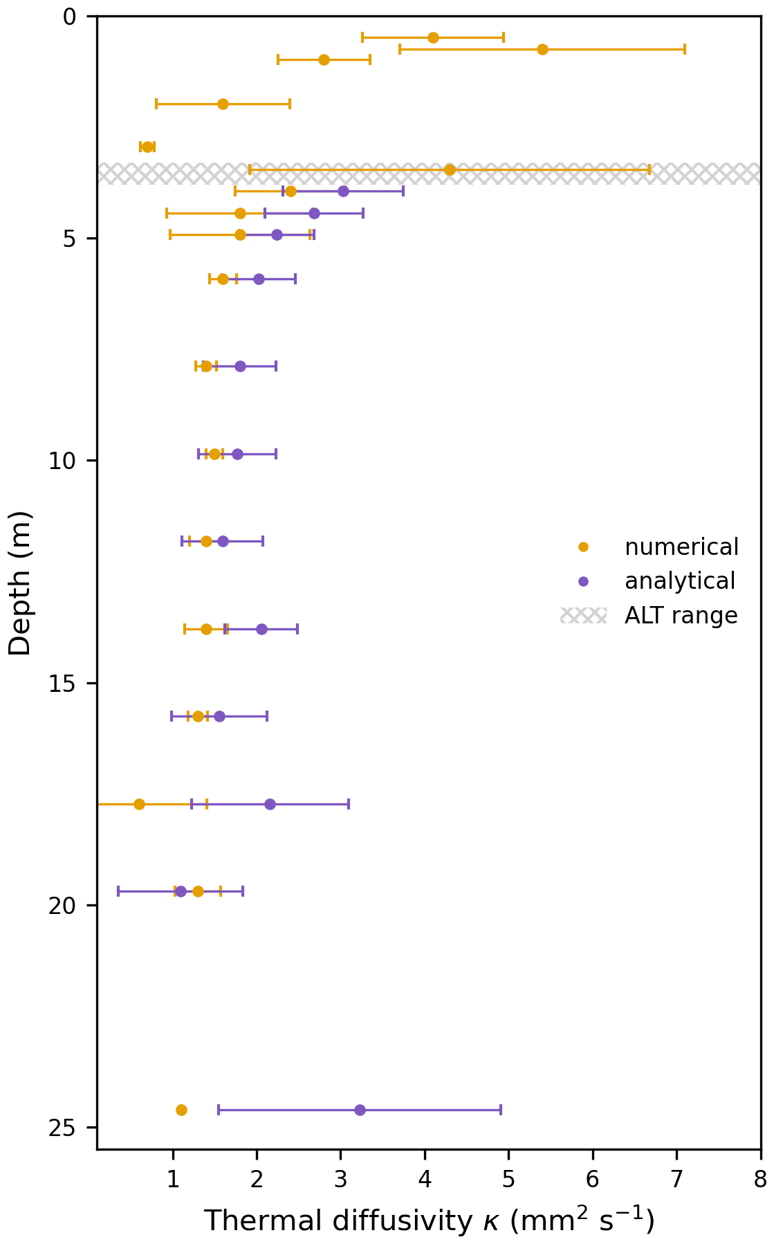
Figure 5 Apparent thermal diffusivity values with depth for borehole COR_0315 on Murtèl-Corvatsch with the numerical and analytical approaches using 12-month windows. The median with the mean absolute deviation is visualized for each sensor down to 25 m depth. The gray area indicates the permafrost table's depth range (active layer depth) over the entire time series. While the analytical solution was only calculated below the maximum active layer depth, the numerically constrained values scatter strongly and vary with depth within the active layer. In the permafrost body, the diffusivity values are overall more stable, with less scattering for both approaches and correspond to the site-specific mean apparent thermal diffusivity values shown in Amschwand et al. (2025, ∼ 2.3 mm² s⁻¹) but slightly higher than in Schneider et al. (2012, ∼ 1.6 mm² s⁻¹).

3.4 Apparent thermal diffusivity in various landforms

In this section, we synthesize the results from both modeling approaches across all PERMOS temperature boreholes, grouped by landform as documented in the PERMOS metadata (data available at https://www.permos.ch/data-portal/permafrost-temperature-and-active-layer, last access: 17 November 2025;  PERMOS, 2024). Thermal diffusivity (κ) values constrained within the permafrost body using numerical inversion and the analytical solution are shown as violin plots in Fig. 6, alongside medians and median absolute deviations. Additionally, median and interquartile ranges (25th–75th percentile) are provided below the figure for each landform and modeling approach. Overall, numerical inversion yields broader variances and interquartile ranges than the analytical solution, in contrast to the illustrative example of borehole COR_0315 on Murtèl-Corvatsch (see Fig. 5). Notably, scatter in bedrock sites is significantly higher than in other landforms, with the exception of the Matterhorn borehole. Although bedrock is typically associated with purely conductive heat transfer, several studies have reported the influence of infiltrating water on borehole temperature time series in permafrost (e.g., Phillips et al., 2016; Mollaret et al., 2019; Haeberli et al., 2023; Noetzli et al., 2024; PERMOS, 2024; Weber et al., 2025a). Schilthorn appears as an outlier in some of the analyses, particularly in the analytical approach. This may be attributed to ground temperatures remaining close to 0 °C and a progressive deepening of the active layer over time, undermining the assumption of a periodic sinusoidal cycle without irregular fluctuations for the analytical model. According to PERMOS (2024), two boreholes at Schilthorn (SCH_5198 and SCH_5200) exhibit conditions that complicate or even prevent the identification of the active layer. In SCH_5198, the active layer likely extends below the lowermost sensor, while in SCH_5200, the ground no longer fully refreezes during winter, indicating the formation of a perennial thaw zone (i.e., a talik, see for example Noetzli et al., 2024). Additionally, the Jungfraujoch borehole (JFJ_0195) stands out as an outlier in the dataset, likely due to its unusual orientation. Positioned subparallel to the rock surface, it is strongly influenced by lateral heat conduction. This deviates from the assumption of predominantly vertical conductive heat transfer along the borehole and likely contributes to the distinct thermal diffusivity estimates observed at this site.

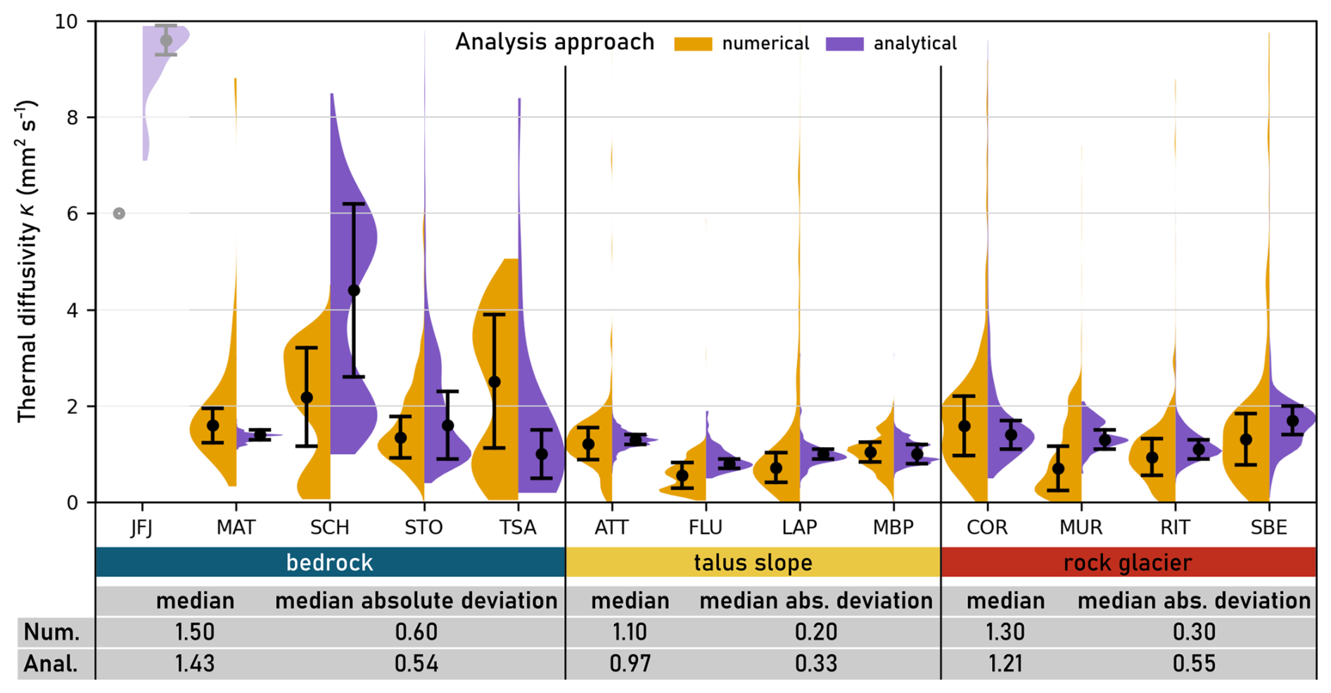
Figure 6 Violin plots of empirically derived thermal diffusivity within the permafrost body (below the active layer) at all PERMOS sites, grouped by landform (explanation of three-character PERMOS abbreviations given in Swiss Permafrost Bulletin 2023; PERMOS, 2024). Median values and median absolute deviations are indicated for each distribution. Boreholes that do not directly capture permafrost conditions (GEM_0106, MUR_0199) and are not located in the landforms bedrock, talus slopes, and rock glaciers (GEN_0102) are not considered. One borehole (JFJ_0195), characterized by an exceptional orientation with dominant lateral heat conduction (due to its position subparallel to the rock surface), is displayed with high transparency and excluded from the statistical summary.

Across all modeling approaches and permafrost landforms, the results indicate typical thermal diffusivity values below the active layer of 1.5 ± 0.6 mm² s⁻¹ for bedrock, 1.1 ± 0.2 mm² s⁻¹ for talus slopes, and 1.3 ± 0.3 mm² s⁻¹ for rock glaciers (median ± median absolute deviation). Although landforms differ considerably in their physical composition, no strong pattern of thermal diffusivity as a function of landform is observed (see Fig. 7). Nevertheless, a statistically significant difference in thermal diffusivity between landforms is found for both modeling approaches (Mann-Whitney U test, p<0.01). On average, thermal diffusivity increases from talus slopes to rock glaciers and is highest in bedrock.

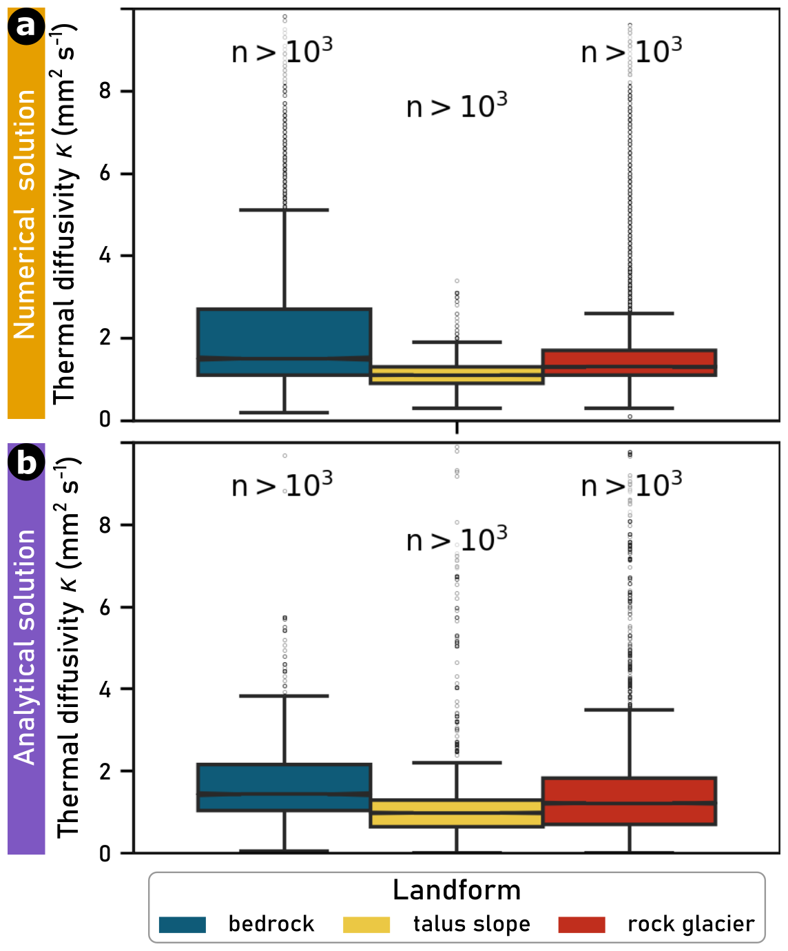
Figure 7 Thermal diffusivity values from all PERMOS boreholes except JFJ_0195, sorted by landform. Values were derived using (a) numerical inversion and (b) the analytical solution of the heat conduction equation. n refers to the number of windows considered in each boxplot.

4 Discussion

In principle, thermal properties of mixed-phase ground materials can theoretically be derived through mixing models and parameterizations (e.g. Cosenza et al., 2003). However, these methods depend on accurate input data regarding ground composition, which are often unavailable for remote mountain permafrost substrates. Additionally, the typically strong heterogeneity of the ground in mountain permafrost areas complicates obtaining a single representative sample. Further, it is very complex or nearly impossible to model all parameters correctly (for example shown by Marmy et al., 2016; Scherler et al., 2014) in such heterogeneous substrates. The novelty of this study lies in the ability to exploit existing measured borehole temperature data to reflect site-specific variability and temporal changes in bulk thermal diffusivity, which are difficult to capture using generalized literature-based estimates or computations. Being aware that field observations and derived parameters often exhibit uncertainties and variability, and that ground temperature and energy balance models rely on input assumptions and are subject to error propagation, we recognize that both approaches are essential and complementary: empirical data help constrain models, while models provide valuable context for interpreting field data. While our study focuses on the quantification of thermal diffusivity as a material parameter, our results suggest that future studies could benefit from integrating these methods to improve both process understanding and predictive capabilities in permafrost thermal modeling.

4.1 Approaches to quantify thermal diffusivity

The simplified heat conduction equation in the differential form allows for the determination of thermal diffusivity based on borehole temperature time series measured at different depths and over time without the assumption of any material properties. This study applies three independent modeling approaches to all 29 PERMOS boreholes distributed across 15 sites and thereby presents a systematic analysis of thermal diffusivity in mountain permafrost. Generally, thermal diffusivity variability decreases with depth. While ground temperatures vary strongly in the active layer, characterized by seasonal fluctuations and phase change resulting in varying water/ice ratios, the temperature tends to approximate thermal conductivity conditions in the permafrost body (see Fig. 5). Due to decreasing temperature variations with increasing depth (see Fig. 1e), temperature change rates typically approach the range of measurement uncertainties around 20 m depth, causing the analysis to lose statistical significance. While sLRM is powerful in short windows of 1–3 months, providing nearly effective thermal diffusivity values, numerical inversion and analytical solution of the heat equation enable to constrain apparent thermal diffusivity in one-year windows. The latter have enabled us for the first time to constrain empirically derived thermal diffusivity values in different permafrost landforms below the active layer. Due to the varying characteristics of mountain permafrost landforms (such as bedrock, talus slopes, and rock glaciers) with different site-specific ground compositions, we also obtain a considerable spread in space and time using all PERMOS borehole temperature time series.

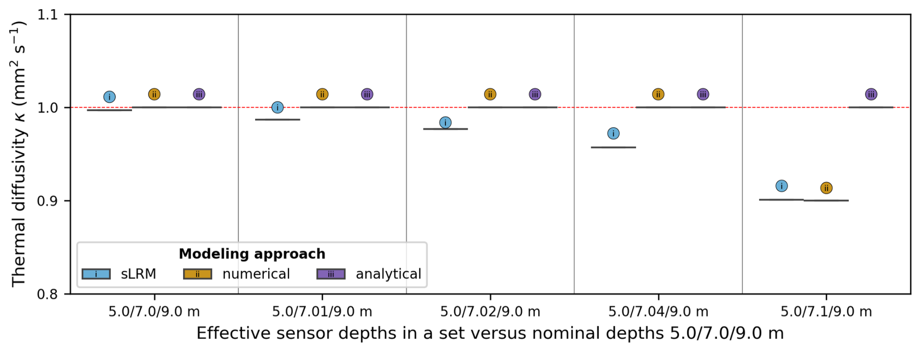
Figure 8 Influence of middle sensor depth accuracy on derived thermal diffusivity values, shown by comparing effective sensor depths (horizontal axis) with the nominal installation depth using the synthetic dataset with predefined thermal diffusivity value of 1 mm² s⁻¹ (indicated by the red horizontal line). Along the x-axis, starting with the reference case, the depth position of the middle sensor is increasingly perturbed, starting from the original depth to a shift of 0.1 m. Each group contains boxplots for each modeling approach with n=55 time steps. While incorrect sensor depths introduce systematic offsets in thermal diffusivity, the results show minimal scatter. This reflects the stable relative positioning of sensors along the borehole chain, even in potentially moving substrates such as talus slopes or rock glaciers.

All three applied modeling approaches constrain the conductive heat exchange along the temperature profile, assuming a horizontally stable thermal regime and homogeneous material properties between the three neighboring sensors. However, in settings where lateral heat fluxes or material heterogeneities are more pronounced, a more comprehensive, multi-dimensional modeling approach would be required to capture the thermal dynamics accurately. For the 1D heat conduction equation, the sLRM is relatively straightforward to implement and requires less computational resources than the numerical solutions. The analytical model is also computationally efficient and is particularly useful for quick estimations. Nevertheless, it relies on simplifying assumptions to derive closed-form solutions of the mathematical equation describing the diffusivity. In nature, conductive heat exchange is highly variable and sometimes superimposed by other heat transfer processes (e.g. Hasler et al., 2011; Amschwand et al., 2025). The validity and the quality of the results of all three modeling approaches are affected by (i) the occurrence of non-conductive processes, (ii) measurement constraints such as the accuracy of the temperature data or the depth of the thermistors, and (iii) analysis parameters such as the temporal window size of the points considered. When dealing with non-uniform sensor spacing, accurately estimating thermal diffusivity using the heat equation becomes particularly challenging for the simple linear regression model (sLRM). This difficulty mainly arises from the numerical approximation of the second spatial derivative, ${\partial }^{\mathrm{2}}T/\partial z^{\mathrm{2}}$. Finite difference schemes typically assume near-uniform spacing between data points, and deviations from this assumption introduce significant inaccuracies in the derivative calculations. Moreover, irregular spacing affects the weighting of data points during interpolation and numerical differentiation, causing unequal influence across the dataset and potentially biasing the results. These inaccuracies in the second derivative propagate through the regression process and compound, ultimately leading to substantial uncertainties and errors in the estimated thermal diffusivity (see Fig. 3). Even though the temperature sensors are fixed along a chain, uncertainties can still arise from inaccurate depth information regarding sensor placement. The influence of middle sensor depth accuracy on the derived thermal diffusivity values is illustrated in Fig. 8 for the synthetic data case. While incorrect sensor depths introduce systematic offsets in thermal diffusivity, minimal spread in each boxplot reflects consistent values for all time steps. Given the stable relative positioning of the sensors along the borehole – ensured by their mounting on the chain – positional errors do not affect the variability associated with κ, even in potentially moving substrates such as talus slopes or rock glaciers.

The sLRM is the most applicable modeling approach for empirically quantifying thermal diffusivity in cold regions where phase changes are suspected (Williams and Smith, 1991; Nicholson and Benn, 2013): Since the rate of temperature change over time ($\partial T/\partial t$) is essentially zero, the assumptions for the linear regression with the temperature Laplacian (${\partial }^{\mathrm{2}}T/\partial z^{\mathrm{2}}$) are violated, and such cases are therefore automatically discarded (see Sect. 2.3). Nevertheless, the sLRM also fails if insufficient measuring points are characterized by pure conductive heat exchange. However, this does not necessarily mean that non-conductive heat flux is present or even dominates, as phase change also influences the temperature profiles and, thus, the model performance. Overall, the thermal diffusivity time series derived from numerical inversion tends to be more complete but needs to be interpreted carefully when the temperature amplitude is getting low and the derived diffusivity values change rapidly or scatter. While the sLRM approach excludes windows containing outliers because the regression assumptions are violated, the numerical inversion can sometimes produce slightly elevated values in isolated time windows affected by short-term non-conductive heat flows. This occurs because the numerical solution attempts to approximate a non-conductive temperature curve using conductive heat transport. Such problematic time windows, where thermal diffusivity tends toward infinity, are usually automatically discarded, as shown in Fig. C2. Nonetheless, we recommend considering the results of the three approaches in combination and, if applicable, considering time windows and depths with matching values for further analyses.

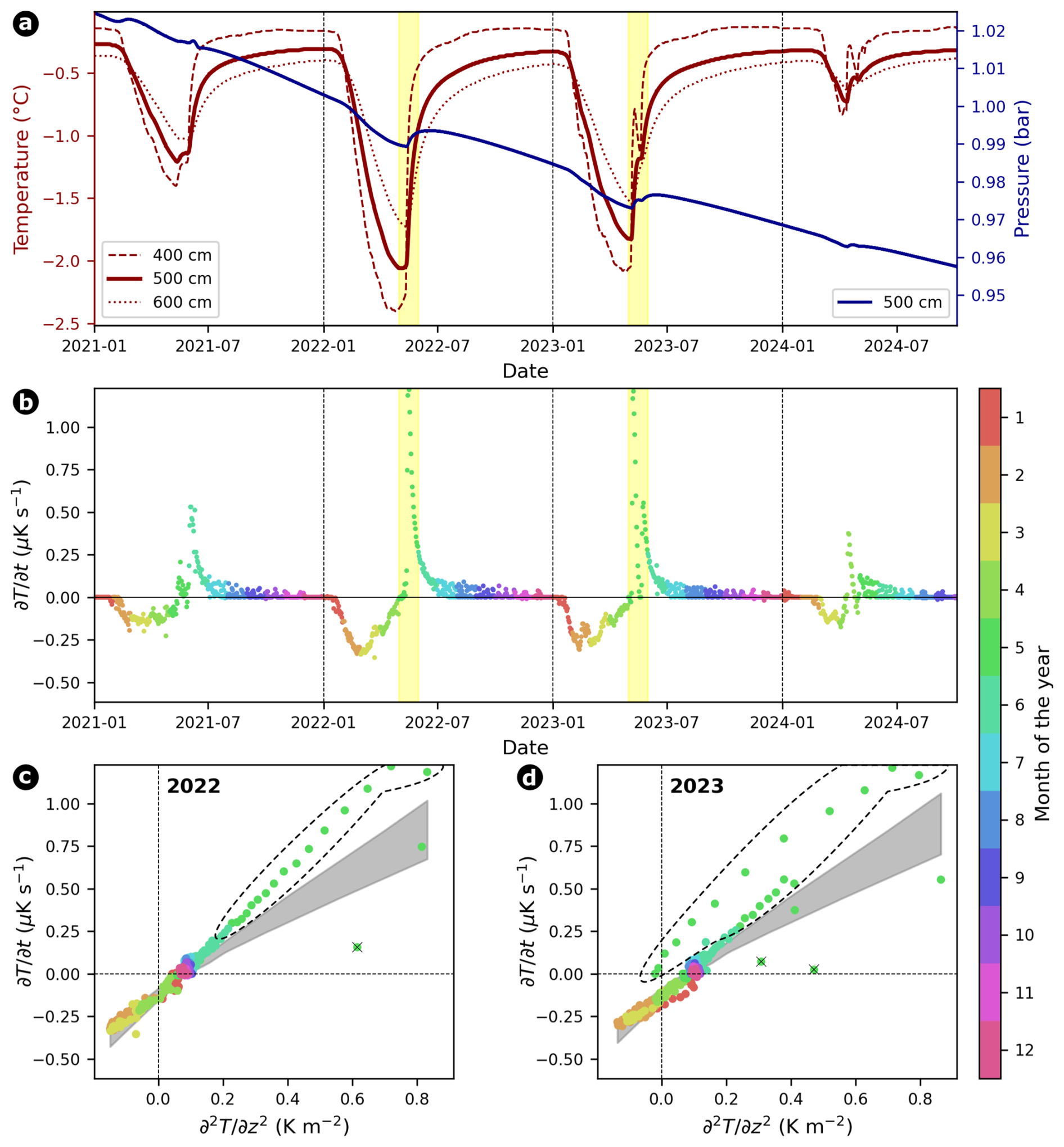
Figure 9 (a) Temperature time series at 4, 5, and 6 m depth, along with piezometric pressure at 5 m, measured in the SLF Schafberg 2020 (SBE_0520) borehole. (b) Rate of temperature change ($\partial T/\partial t$) over the full observation period. (c, d) Scatter plots of temperature change rate versus temperature Laplacian at 5 m depth, focusing on the years 2022 and 2023 with distinct increases in both temperature and water pressure. Individual observations are colored by month, and 95 % prediction bands from all valid linear regression models are represented with a gray area. Selected anomalies are marked with a dashed line in (c) and (d) corresponding to the yellow bars in (a) and (b), coinciding with distinct increases in both temperature and pressure at 5 m, indicative of short-term non-conductive heat fluxes.

4.2 Thermal diffusivity: beyond a model parameter

Our findings improve the understanding of thermal behavior in mountain permafrost and provide direct implications for ground temperature and energy balance modeling, as well as applied studies such as extracting ground composition and isolating short-term non-conductive heat fluxes. The sLRM approach also provides valuable by-products, such as the detection of sensor drift (e.g., Schafberg, for details see  Luethi and Phillips, 2016; Haberkorn et al., 2021). Thermistors are susceptible to gradual drift over time, which can be challenging to identify apart from the active layer with zero curtain periods, particularly during periods of rising ground temperatures, when such changes may be mistaken for genuine environmental trends. Sensor drift can distort the relation between the rate of temperature change and the temperature Laplacian, as the Laplacian depends on data from neighboring thermistors. Thereby, the sLRM procedure can serve as a quantitative indicator of previously undetected sensor drift, adding an essential layer of quality control to the analysis.

In the following, we outline the need for and benefit of site-specific, empirically derived thermal diffusivity values for applied studies and discuss potential applications of our approach.

4.2.1 Non-conductive heat fluxes

Non-conductive heat fluxes, such as heat advection and convection by deep water infiltration are of particular interest as they can lead to accelerated warming of the ground, which can cause several problems, for example, inducing deep-seated slope instabilities or complicating construction work. So far, efforts have been made to detect non-conductive heat fluxes in mountain permafrost, aiming to determine their timing, depth, and duration. Amongst others, anomalies in spectral analysis of temperature time series (Hinkel and Outcalt, 1993; Hasler, 2011), simulations with different heat sources and sinks (Luethi et al., 2017), temperature contour plots showing flags in the 0 °C isotherm (e.g., Luethi and Phillips, 2016), or outliers and jumps in the temperature time series (Phillips et al., 2016; Offer et al., 2024) appear to be promising indicators for non-conductive heat fluxes. However, there are only qualitative indications based on manual selection.

We postulate that the sLRM approach enables the investigation of non-conductive processes governed by thawing and/or water advection at any location with a temperature borehole. Given the one-dimensional heat conservation equation, we suggest identifying the occurrence of short-term non-conductive heat fluxes – a proxy for water or air circulation – by comparing the observations and model prediction of temperature rate variations over time and isolating spatio-temporal anomalies. For verification, we apply our approach to an additional borehole, namely the SLF Schafberg 2020 (SBE_0520) borehole (time series of temperature, piezometric pressure and temperature rates are shown in Fig. 9) to demonstrate that we observe a coincident increase in piezometric pressure. Although thermal diffusivity changes in space and time, we can indirectly identify short-term periods with non-conductive processes: First, we combine observed temperature rates ($\partial T/\partial t$, dots colored by month) with the 95% prediction band (gray area) of the sLRM across the temperature Laplacian (see Fig. 9c, d for the years 2022 and 2023). Then, we drop observations that do not show a considerable deviation from the $\partial T/\partial t$ zero line as the period might be governed by phase changes (see black crosses on top of green dots). Finally, we select observations that lie outside the model prediction band (e.g., most green dots in Fig. 9c, d) and interpret them as temporary periods governed by advective processes.

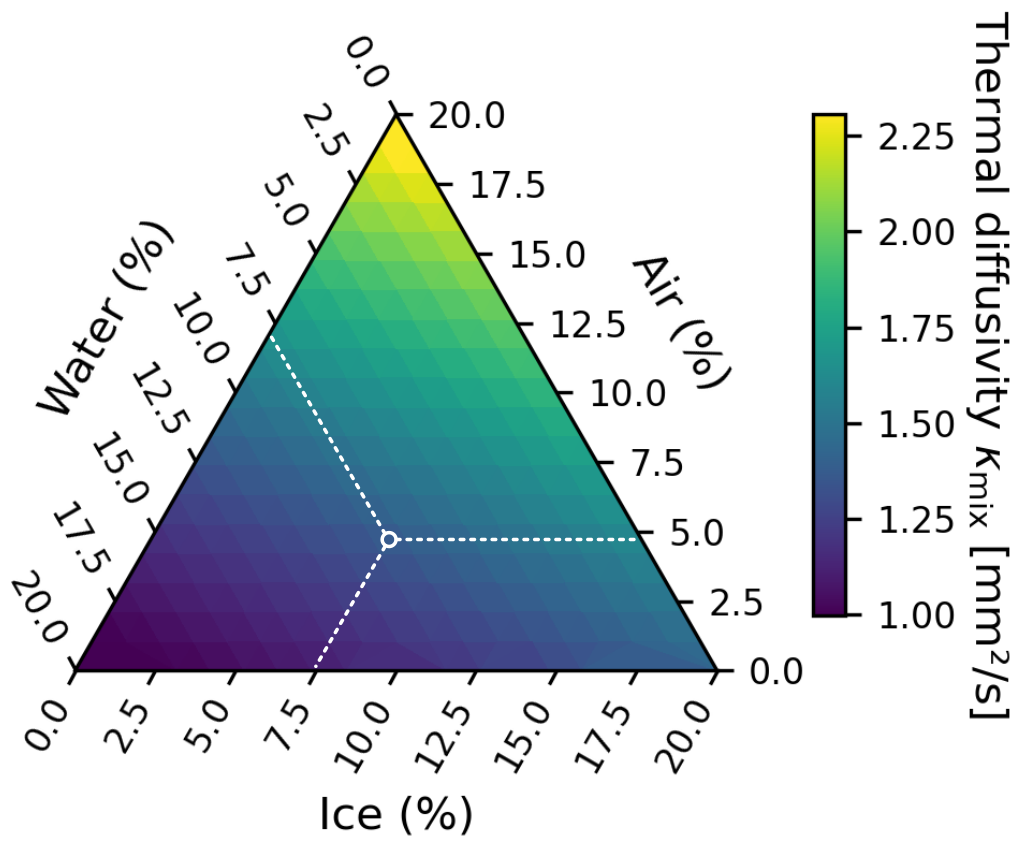
Figure 10 Ternary diagram showing the thermal diffusivity κ_mix of a four-component ground mixture based on the geometric mean model (Tatar et al., 2021). The volumetric rock fraction is fixed at 80 % (granite with $\mathit{\kappa }=\mathrm{1.5}{\mathrm{mm}}^{\mathrm{2}}{\mathrm{s}}^{-\mathrm{1}}$), and the remaining 20 % of the volume is distributed among ice ($\mathit{\kappa }=\mathrm{1.16}{\mathrm{mm}}^{\mathrm{2}}{\mathrm{s}}^{-\mathrm{1}}$), water ($\mathit{\kappa }=\mathrm{0.14}{\mathrm{mm}}^{\mathrm{2}}{\mathrm{s}}^{-\mathrm{1}}$), and air ($\mathit{\kappa }=\mathrm{16.57}{\mathrm{mm}}^{\mathrm{2}}{\mathrm{s}}^{-\mathrm{1}}$). Each point in the triangle corresponds to a unique composition of the non-rock components, with coloring representing the resulting thermal diffusivity of the four-component ground mixture. The white circle and the white dashed lines indicate a possible combination for the remaining 20 %. This visualization enables comparison between empirically derived thermal diffusivity values and theoretically plausible ground compositions or, inversely, the extraction of ground composition through the comparison of observed values with established thermal properties of distinct materials.

The sLRM approach offers a cost-effective method for identifying short-term, non-conductive heat fluxes in mountain permafrost. It is simpler and cheaper to implement than the challenging measurements of water content or pressure, and it provides a more robust alternative to detecting short-term jumps in temperature typically caused by water infiltration (e.g., from snow melt) that are visible in summer 2023 but not in summer 2022 (see Fig. 9a). The identification of non-conductive processes thereby provides information on the timing and intensity of relevant heat transport processes (McKenzie and Voss, 2013). Ideally, heat transfer and water flow should be treated as fully coupled processes with interrelated physics, an approach that has been theoretically applied to polar permafrost but not yet fully validated with hydrogeological field data (Kurylyk and Walvoord, 2021). However, modeling groundwater flow in mountain permafrost remains challenging due to complex topography, heterogeneous subsurface conditions, variable ice and water contents, changing permeabilities, and very limited water flow measurements (e.g. Scandroglio et al., 2025).

4.2.2 Estimating ground composition from thermal diffusivity

Using empirically derived thermal diffusivity, we can extract ground composition by comparing the observed values with the known thermal properties of individual materials (rock, ice, air, and water) and their mixtures (see Table 1). Estimating the volumetric fraction of rock (V_rock), the application of a mixing model, such as the weighted geometric mean model (e.g., Tatar et al., 2021), allows for the calculation of the thermal diffusivity κ_mix by weighting the thermal diffusivity of each component (rock, ice, water, and air) by its respective volumetric fraction. Each constituent is characterized by a predefined thermal diffusivity. The thermal diffusivity of the four-component system is then calculated as

$$\begin{array}{}\text{(11)}& {\mathit{\kappa }}_{\text{mix}}={\mathit{\kappa }}_{\text{rock}}^{V_{\text{rock}}}\cdot {\mathit{\kappa }}_{\text{ice}}^{V_{\text{ice}}}\cdot {\mathit{\kappa }}_{\text{water}}^{V_{\text{water}}}\cdot {\mathit{\kappa }}_{\text{air}}^{V_{\text{air}}}\end{array}$$

subject to the constraint

$$\begin{array}{}\text{(12)}& V_{\text{rock}}+V_{\text{ice}}+V_{\text{water}}+V_{\text{air}}=\mathrm{1}.\end{array}$$

Compared to the linear volumetric mixing law (arithmetic mean model, ${\mathit{\kappa }}_{\text{mix}}=V_{\text{rock}}\cdot {\mathit{\kappa }}_{\text{rock}}+V_{\text{ice}}\cdot {\mathit{\kappa }}_{\text{ice}}+\mathrm{\dots }$), the geometric mean model is often considered as being more physically representative for heterogeneous porous materials, especially when the components differ significantly in thermal diffusivity (Preux and Malinouskaya, 2021). In such media, heat flow is not evenly distributed through each phase; instead, it tends to follow preferential paths through more conductive materials. The geometric mean accounts for this behavior better by emphasizing the impact of low-diffusivity components, such as air, which can strongly reduce the thermal diffusivity even at small volumetric fractions. This approach thus provides a more realistic estimation of thermal transport properties in partially saturated ground or ground containing air typical of permafrost-affected terrain.

Given a realistic estimated V_rock, for example 80 %, the remaining 20 % of the volume is distributed among ice, water, and air (porosity model where one of the four unknowns is prescribed, comparable to Hauck et al., 2011). All possible combinations of these three components can be represented in a ternary plot (triangle diagram), where each point corresponds to a unique composition of the remaining non-rock volume. For each combination, κ_mix is computed and visualized as contours within the ternary space (see Fig. 10). Overlaying the empirically derived thermal diffusivity enables the identification of plausible ground compositions that match the observed values. This approach allows for a physically meaningful interpretation of thermal properties in terms of ice content, water saturation, and porosity. It bridges empirical measurements with theoretical ground compositions, providing insights into the thermal, hydrological, and structural state of the subsurface. This is particularly valuable in mountain permafrost environments, where ground composition strongly influences thermal and mechanical behavior as well as sensitivity to climate.

5 Conclusions and Outlook

We implemented three mathematically independent formulations of the differential heat conduction equation in Python 3 (Weber et al., 2025b, an open-source Python 3 module) to infer thermal diffusivity from temperature profiles: (i) simple linear regression model (sLRM, statistical estimation), (ii) numerical inversion (semi-implicit finite-difference model), and (iii) analytical solution (explicit calculation). We proved their validity and performance with synthetic data. The systematic analysis of the 29 borehole temperature time series of the Swiss Permafrost Monitoring Network (PERMOS) then enabled us to constrain thermal diffusivity in mountain permafrost landforms below the active layer without assuming any material properties to 1.5 ± 0.6 mm² s⁻¹ for bedrock, 1.1 ± 0.2 mm² s⁻¹ for talus slopes, and 1.3 ± 0.3 mm² s⁻¹ for rock glaciers (median ± median absolute deviation).

These values directly benefit a variety of models, amongst others, for ground temperature distributions or energy balance estimates, even in the absence of boreholes, either as input data or for calibration purposes. Supposing a borehole with temperature sensors exists, regardless of the ground material, the developed approaches to empirically quantify diffusive heat exchange can be applied, constituting a valuable foundation for further permafrost studies. The derived site-specific and depth-resolved thermal diffusivity time series can serve two important purposes: (i) they can be coupled with surface energy balance models to simulate ground heat transport better, and (ii) they offer valuable insights into the temporal evolution of the ground composition linked to changes in water content or the physical state of water and the related ice/water ratio (see Sect. 4.2.2), for example in response to seasonal or long-term climate variations. Therefore, site-specific seasonal temperature patterns and possible shifts or alterations thereof can be a valuable addition to other prospecting methods to track changes in ground composition/properties, which are a prerequisite for reliable thermo-mechanical stability analyses and modeling in a changing climate.

Additionally, we have developed an indirect approach for such locations to empirically identify and investigate non-conductive processes driven by thawing and/or water advection. This is done by isolating spatial and temporal anomalies in the relation between the temperature Laplacian and the temperature change rate, where the regression coefficient corresponds to thermal diffusivity. Further development of this approach could allow us to quantify non-conductive heat flux based on the energy conservation equation. Thus, this study lays the foundation for investigating the thermal and mechanical behavior of mountain permafrost slopes. For instance, the site-specific ratio of available energy dissipated through turbulent fluxes can be estimated by combining conductive heat fluxes, calculated from thermal diffusivity and borehole temperature data, with net radiation measurements.

Appendix A: Calculation of the temperature Laplacian

To estimate the temperature Laplacian ${\partial }^{\mathrm{2}}T/\partial z^{\mathrm{2}}$, geometrically meaning the spatial curvature of the temperature profile, we approximate the second derivative of temperature with respect to depth using a finite difference scheme. Based on the discrete vertical temperature measurements from borehole sensors, the second derivative is computed as the difference of first-order forward differences, normalized by the vertical distance between the segments. The resulting expression for the second derivative is given by

$$\begin{array}{}\text{(A1)}& {\partial }^{\mathrm{2}}T/\partial z^{\mathrm{2}}\approx -{\displaystyle \frac{\mathrm{1}}{\mathrm{\Delta }{z}_{i+\mathrm{1}/\mathrm{2}}}}\left({\displaystyle \frac{T_{i+\mathrm{2}}-T_{i+\mathrm{1}}}{\mathrm{\Delta }{z}_{i+\mathrm{1}}}}-{\displaystyle \frac{T_{i+\mathrm{1}}-T_i}{\mathrm{\Delta }{z}_i}}\right)\end{array}$$

here, T_i denotes the temperature at sensor i, Δz_i and Δz_i+1 are the vertical distances between adjacent temperature sensors, and $\mathrm{\Delta }{z}_{i+\mathrm{1}/\mathrm{2}}$ is the distance between the midpoints of the corresponding vertical intervals. The negative sign is introduced to ensure consistency with the curvature direction expected from the second derivative. This formulation allows us to account for non-uniform sensor spacing commonly encountered in borehole installations.

Alternative methods, such as computing ${\partial }^{\mathrm{2}}T/\partial z^{\mathrm{2}}$ from cubic spline interpolation of the temperature profile, were tested but did not improve accuracy or robustness compared to the finite difference approach. They are therefore not pursued further in this study.

Appendix B: Generation of synthetic dataset

Analytically generated synthetic temperature datasets were created to represent purely conductive heat transfer conditions, following the characteristics of borehole COR_0315 on Murtèl-Corvatsch. The models assume thermal diffusivities of κ=1 and $\mathit{\kappa }=\mathrm{5}{\mathrm{mm}}^{\mathrm{2}}{\mathrm{s}}^{-\mathrm{1}}$, a constant geothermal heat flux of 50 mW m⁻² for initial temperature distribution down to 17 m depth, and a sinusoidal surface temperature forcing with a mean annual ground surface temperature (MAGST) of −2.5 °C and an annual surface amplitude of 10 °C. The temperature distribution is computed using the analytical solution to the one-dimensional heat conduction equation with periodic surface forcing:

$$\begin{array}{}\text{(B1)}& T(z,t)={\stackrel{\mathrm{‾}}{T}}_{z=\mathrm{0}}+A_{\mathrm{s}}\cdot e^{-z(\mathit{\omega }/\mathrm{2}\mathit{\kappa }{)}^{\mathrm{1}/\mathrm{2}}}\cdot \sin \left[\mathit{\omega }t-z\cdot {\left(\mathit{\omega }/\mathrm{2}\mathit{\kappa }\right)}^{\mathrm{1}/\mathrm{2}}\right],\end{array}$$

where ${\stackrel{\mathrm{‾}}{T}}_{z=\mathrm{0}}$ is the mean annual ground surface temperature, A_s the amplitude of the surface temperature variation, z the depth, t the time, $\mathit{\omega }=\mathrm{2}\mathit{\pi }/\mathit{\tau }$ the angular frequency, and $\mathit{\tau }=\mathrm{1}\mathrm{year}=\mathrm{31}\mathrm{536}\mathrm{000}\mathrm{s}$. Each dataset spans depths from 5 to 17 m, representing the permafrost body below the active layer, and covers two full years at daily resolution – exemplarily shown in Fig. B1 for $\mathit{\kappa }=\mathrm{1}{\mathrm{mm}}^{\mathrm{2}}{\mathrm{s}}^{-\mathrm{1}}$. As expected, increasing thermal diffusivity leads to deeper penetration of the seasonal signal and reduced phase lag with depth. These synthetic datasets serve as controlled benchmarks for testing and evaluating numerical approaches to estimate thermal diffusivity in permafrost environments.

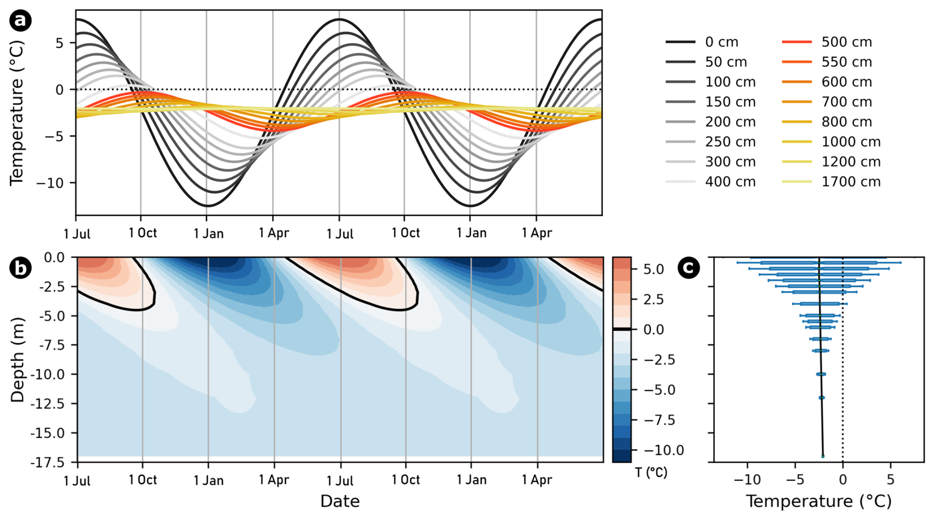
Figure B1 Example of the analytically generated synthetic dataset with predefined thermal diffusivity value of 1 mm² s⁻¹, mean annual ground surface temperature of −2.5 °C, and an annual amplitude of 10 °C. (a) The annual course over two years for different depths in the active layer (gray colors between 0 and 4 m depth) and in the underlying permafrost (between 5 and 17 m depth). (b) Temperature contour plot over the entire depth and (c) temperature profile along the synthetic borehole, illustrating the active layer's seasonal freeze/thaw cycles and the decreasing annual amplitude with increasing depth.

Appendix C: Visual assessment of methodological approaches

This appendix provides (i) examples of a diagnostic diagram to check the assumptions for linear regression analysis (Fig. C1), and (ii) the performance of sLRM analysis and numerical inversion when phase changes or non-conductive heat fluxes occur (Fig. C2).

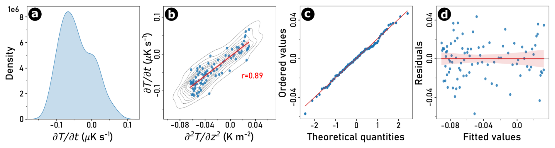
Figure C1 Diagnostic plots used to prove the assumptions for linear regression analysis between IV (independent variable) and DV (dependent variable) – as an illustrative example, borehole COR_0315 on Murtèl-Corvatsch at a depth of 10 m and within the time window from 22 April to 22 July 2016: (a) Normal distribution of predictors, (b) linear relation between the DV and the IV, (c) normality of the residual errors to confirm that both datasets (DV and IV) have a common distribution (all points of quantiles should lie on or close to a straight line with a gradient of 1), and (d) homoscedasticity (or equal variance) of residuals (spread of the residuals from the linear regression model should be homogeneous or equal spaces).

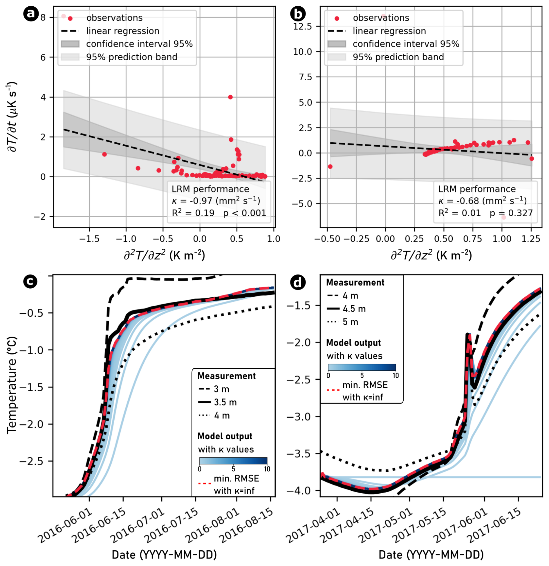
Figure C2 Exemplary 3-month time windows at borehole COR_0315 on Murtèl-Corvatsch show that the sLRM (a–b) and the numerical inversion (c–d) approaches fail during periods characterized by phase change (a and c; e.g. at 3.5 m depth from 17 May to 17 August 2016) or non-conductive heat fluxes (b and d; e.g. at 4.5 m depth from 25 March to 25 June 2017).

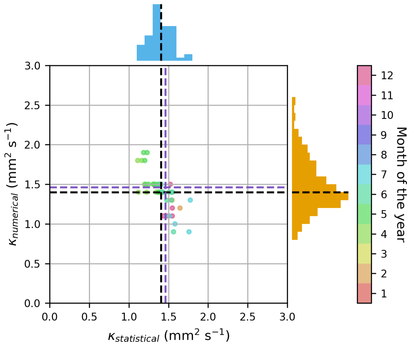
Figure C3 A comparison of thermal diffusivity for borehole COR_0315 on Murtèl-Corvatsch at 10 m depth derived through linear regression analysis of the heat conduction equation and inversions of numerical and analytical solutions within a 3-month window. While the scattering of both approaches is normally distributed, their means (dashed black lines) and the mean of the analytical solution in a 12-month window (purple dashed line) are comparable (± 0.1 mm² s⁻¹).