Object-based ensemble estimation of snow depth and snow water equivalent over multiple months in Sodankylä, Finland

Snowpack characteristics such as snow depth and snow water equivalent (SWE) are widely studied in regions prone to heavy snowfall and long winters. These features are measured in the field via manual or automated observations and over larger spatial scales with stand-alone remote sensing methods. However, individually these methods may struggle with accurately assessing snow depth and SWE in local spatial scales of several square kilometers. One method for leveraging the benefits of each individual dataset is to link field-based observations with high-resolution remote sensing imagery and then employ machine learning techniques to estimate snow depth and SWE across a broader geographic region. Here, we combined field-based repeat snow depth and SWE measurements over six instances from December 2022 to April 2023 in Sodankylä, Finland with Light Detection and Ranging (LiDAR) and WorldView-2 (WV-2) data to estimate snow depth, SWE, and snow density over a 10 km² local scale study area. This was achieved with an object-based machine learning ensemble approach by first upscaling more numerous snow depth field data and then utilizing the estimated local scale snow depth to aid in estimating SWE over the study area. Snow density was then calculated from snow depth and SWE estimates. Snow depth peaked in March, SWE shortly after in early April, and snow density at the end of April. The ensemble-based approach had encouraging success with upscaling snow depth and SWE. Associations were also identified with carbon- and mineral-based forest surface soils, alongside dry and wet peatbogs.

1 Introduction

Seasonal snow is found in regions of the globe that experience freezing temperatures and is widely studied to monitor changes in climate and hydrology. Snow is a component of the cryosphere that is heterogeneous over space and time. Snowmelt provides drinking and irrigation water to approximately one sixth of the world's population (Barnett et al., 2005). The initial layering of the snowpack is impacted by the deposition of falling snow, windblown snow redistribution, or a combination of the two (Nienow and Campbell, 2011). Further densification can occur due to compaction and metamorphic mechanisms, alongside meltwater, percolation, and refreeze events (Prowse and Owens, 1984; Tuttle and Jacobs, 2019; El Oufir et al., 2021; Colliander et al., 2023). Given these factors, key elements of snow density are the age of the snowpack, snow depth, and water content. Fresh snow can have a snow density of 0.05–0.07 g cm⁻³ while fresh damp snow can range from 0.10–0.20 g cm⁻³ (Muskett, 2012). In contrast, the snow density of older dry snow is roughly 0.35–0.40 g cm⁻³ and for older wet snow is up to 0.50 g cm⁻³ (Seibert et al., 2015). Very wet snow and firn, which is snow that failed to melt in the previous summer and did not turn into ice, can contain a snow density ranging from 0.40–0.80 g cm⁻³ (Muskett, 2012; Arenson et al., 2021). Within the Northern Hemisphere, there is an immense variation in average snow density which ranges from 0.05–0.59 g cm⁻³ with an overall long-term average snow density of 0.25±0.07 g cm⁻³ (Zhao et al., 2023).

Despite the attainability of snow density classification, there are significant complexities with generating the estimated snow density alongside the related snow depth and snow water equivalent (SWE) over large areas and in challenging environments such as thick forests and mountainous terrain. Snow depth is simply the total depth of snow on the ground while SWE can be defined as the resulting depth of water produced from the complete melt of a mass of snow (Henkel et al., 2018). The quantity of SWE is determined by the amount of snow accumulation alongside the amount of snow melt and sublimation (Xu et al., 2019). Field-based SWE datasets are both spatially and temporally scarce and can be expensive and labor intensive to acquire (Henkel et al., 2018; Fontrodona-Bach et al., 2023). In contrast, field-acquired snow depth measurements are more common, and are both easier and faster to obtain, though their spatial extent is also limited and can be challenging to obtain in difficult or remote areas (Collados-Lara et al., 2020; Tanniru and Ramsankaran, 2023). Automated stations can be utilized to collect snow measurements, which are rapidly becoming more commonplace, such as accounting for over 80 % of the snow depth observing network north of 55° N in Canada (Brown et al., 2021). However, such stations may sometimes be primarily intended for non-climatic purposes such as for avalanche warnings and thus not be verified nor corrected for climatic trends (Salzmann et al., 2014).

Alternatives to field-based methods of snow observations are the use of airborne and spaceborne sensors to estimate snow properties which have achieved great success in recent decades (Nagler and Rott, 2000; Kelly et al., 2003; Marti et al., 2016; Cimoli et al., 2017; Tsai et al., 2019). Such sensors achieve large spatial coverage and the ability to clearly differentiate between snow and non-snow features (Nolin, 2010; Raghubanshi et al., 2023). However, many commonly used spaceborne sensors such as with the Landsat series, the Moderate Resolution Imaging Spectroradiometer (MODIS), the Advanced Very High Resolution Radiometer (AVHRR), and the Advanced Microwave Scanning Radiometer (AMSR-E/AMSR2) have limitations. These are either not capable of directly estimating snow depth or SWE, or, if able, have limited penetration or contain very coarse resolutions that make local scale estimation unattainable, in addition to potential cloud cover contamination (Rodell and Houser, 2004; Green et al., 2012; Lu et al., 2022; Stillinger et al., 2023). Repeat images captured via airborne Light Detection and Ranging (LiDAR) can serve to successfully estimate changes in snow depth (Deems et al., 2013; King et al., 2023); however, the flights needed for these are costly, weather dependent, and require trained pilots and LiDAR specialists (Jacobs et al., 2021; Yu et al., 2022). While issues are present in relying solely on remote sensing for snow depth and SWE estimation, a blending of remote sensing imagery and field-based snow data can serve to significantly improve snow depth and SWE estimations (Kongoli et al., 2019; Pulliainen et al., 2020; Cammalleri et al., 2022; Venäläinen et al., 2023).

In addition to this, the inclusion of machine learning can expand the potential to estimate snow depth and SWE over spatial and temporal scales. Machine learning techniques have been successfully applied to predict such features across Earth, including high altitude and high latitude environments (Jonas et al., 2009; Bair et al., 2018; King et al., 2020; Zhang et al., 2021; Shao et al., 2022; Hu et al., 2023). Commonly employed algorithms including Artificial Neural Network (ANN), K-Nearest Neighbor (KNN), Multiple Linear Regression (MLR), Random Forest (RF), and Support Vector Machine (SVM) have achieved success in snow depth, SWE, and snow-liquid ratio estimations (Broxton et al., 2019; Douglas and Zhang, 2021; Ntokas et al., 2021; Vafakhah et al., 2022; Hoopes et al., 2023; Liljestrand et al., 2024). Deep learning models such as Convolutional Neural Networks (CNNs) have also successfully been employed to estimate snow cover, snow depth, and SWE at various scales across the globe (Nijhawan et al., 2019; Xing et al., 2022; Duan et al., 2024; Kesikoglu, 2025). Individually many of these algorithms can produce positive results, though there may be a tendency for disagreement in model accuracy and outcomes (Li et al., 2023). As an alternative, a weighted ensemble-based empirical model can be utilized to potentially increase model accuracy, while also reducing estimation error (Douglas and Zhang, 2021; Brodylo et al., 2024). As each algorithm is optimized differently to generate outputs, each containing their pros and cons, an ensemble approach can improve feature estimation to ensure optimal results (Pes, 2020). A combination of such machine learning models, remote sensing imagery, and field-based snow data can thus provide the necessary foundations to map snow features across the cryosphere, which has been experiencing rising temperatures and increasing climatic uncertainty (Pan et al., 2017; Yang et al., 2020; Santi et al., 2022).

One region where application of such a technique is worthwhile is in northern Europe, particularly in the Lapland region located largely within the Arctic Circle. The area around Sodankylä, Finland is prone to long, cold winters with abundant snowfall and both on-the-ground snow depth and SWE measurements are available for multiple months or more. Here, we sought to utilize an object-based hybrid deep learning and machine learning ensemble approach with a combination of time-series field and automated snow data, alongside WorldView-2 (WV-2) imagery and LiDAR data to upscale snow depth, SWE, and snow density to a 10 km² local scale. This was implemented over six instances from December 2022 to April 2023, with snow estimates matched to dominant vegetative communities. Field-based snow depth observations were upscaled first, before utilizing the estimated snow depth to aid in upscaling more limited SWE field data to the local scale, with snow density then being mapped. Distinctive machine learning algorithms were employed and compared to an ensemble-based technique for both snow depth and SWE estimation.

2 Study area and data

2.1 Study area

The study area is found near the town of Sodankylä in the Sodankylä municipality of northern Finland, which is roughly 125 km north of the Arctic Circle. The 10 km² site is located along the Kitinen River and hosts the Finnish Meteorological Institute Arctic Space Centre (FMI-ARC) and the Sodankylä Geophysical Observatory (Bösinger, 2021) between 67.356° N, 26.609° E, and 67.381° N, 26.693° E (Fig. 1). It is largely flat, with elevations ranging between 170 and 190 m above sea level. Landcover consists primarily of coniferous and deciduous dominated forests and peat bogs, contains organic and mineral soils, and portrays a standard flat northern boreal forest/taiga setting (Rautiainen et al., 2014). Field analysis revealed a multitude of vegetative species at the study site. Dominant tree species are Betula pubescens (downy birch) and Pinus sylvestris (Scots pine). Common shrub species include Andromeda polifolia (bog rosemary), Empetrum nigrum (crowberry), Rhododendron tomentosum (Labrador tea), Vaccinium cespitosum (dwarf bilberry), Vaccinium myrtillus (bilberry), Vaccinium oxycoccus (cranberry), and Vaccinium vitis-idaea (lingonberry). Graminoid species were comprised of Carex lasiocarpa (woollyfruit sedge), Danthonia decumbens (heath grass), Eriophorum vaginatum (tussock cottongrass), Scheuchzeria palustris (pod grass), and Trichophorum cespitosum (tufted bulrush). Forb species include Comarum palustre (purple marshlock) and Menyanthes trifoliata (bog bean). Lichen and moss are also common.

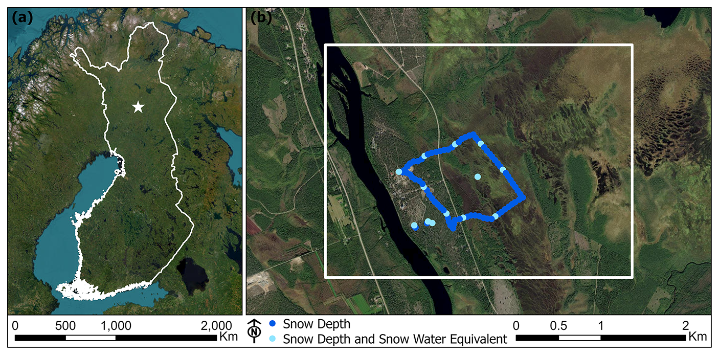
Figure 1 Study area (a) in Sodankylä, Finland and (b) automated and manual snow depth and snow water equivalent measurements within the 10 km² local scale study site. Image credits: Esri, Earthstar Geographics, and Maxar.

The climate in Sodankylä is defined by short but relatively warm summer season and a long and cold winter, with snow present from October to May. Taiga snow is dominant, with thick layering of depth hoar at the base of the snowpack (Anttila et al., 2014). Meaningful rain-on-snow events occur in November and early December (Bartsch et al., 2023). Between 1991 and 2020 at the FMI Sodankylä Tähtelä weather station, the average yearly precipitation was 543 mm with an average yearly maximum snow depth of 91 cm that ranged from 65–127 cm. The average air temperature was 0.4 °C, the average minimum was −4.2 °C, and the average maximum was 4.8 °C. The absolute minimum temperature was −49.5 °C while the absolute maximum was 32.1 °C. The mean annual air temperature has increased by 0.07 °C from 2000–2018 (Bai et al., 2021) and is expected to continue. Between the winters of 2007/08 to 2013/14 around FMI-ARC and the Sodankylä Geophysical Observatory, the maximum SWE ranged approximately from 150–250 mm (Essery et al., 2016). For the winter of 2022/23, a maximum snow depth of 99 cm was recorded at the Sodankylä Tähtelä weather station on 31 March 2023, with rapid snow melt in April and early May (Fig. 2). The average air temperature was generally near or below freezing in winter and contained relatively low precipitation. The site generally contains low wind speeds that limit windblown snow redistribution, with a monthly average of 2.5–2.9 m s⁻¹ above the forest canopy (Meinander et al., 2020).

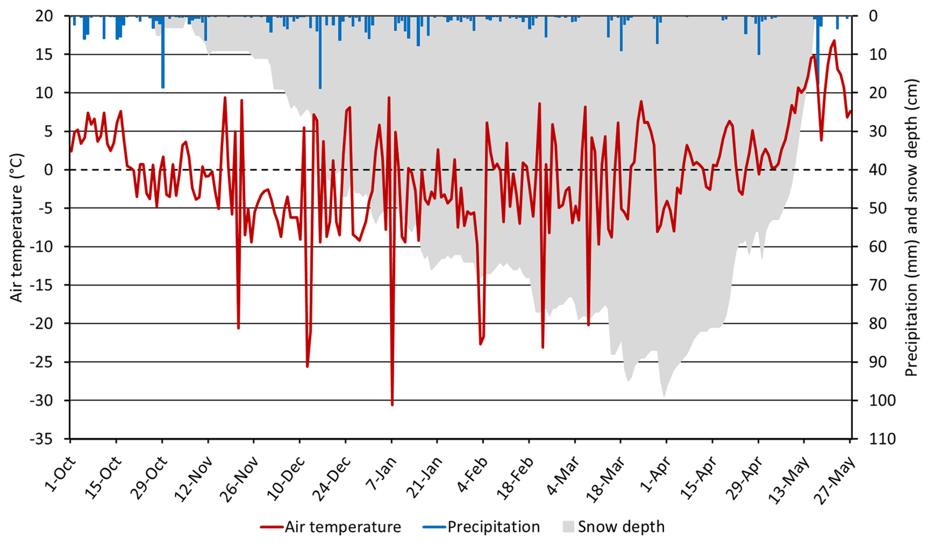
Figure 2 Daily average air temperature (°C), precipitation (mm), and snow depth (cm) from the FMI Sodankylä Tähtelä weather station from 1 October 2022–27 May 2023.

2.2 Ground-based and remotely sensed measurements

Field-based snow data were acquired over distinct vegetative communities on 14 December 2022, 17 January 2023, 15 February 2023, 17 March 2023, 17 April 2023, and 28 April 2023. Manually obtained snow depth was measured with a fixed stake or manual probe, while SWE was calculated with a scale that is paired to a snow tube that is 70 cm high and 10 cm in diameter that includes a scale on the outside to measure snow depth (Leppänen et al., 2016). Automated observations were performed for snow depth with the Campbell Scientific SR50 sonic distance instrument and for SWE with the Sommer Messtechnik SSG 1000 snow scale instrument. A total of 88 repeat snowpack depth (cm) measurements were taken at the same locations with 80 being manually recorded and 8 being acquired from automated stations (Fig. 1b). Of these same 88 locations, a total of 13 repeat SWE (mm) measurements were recorded: 11 manually and 2 from automated stations. SWE values were based on the total snowpack depth. An average daily value was recorded from the automated stations to match with the field-based observations, with previously strong correlations found between the automated and manual measurements for both snow depth and SWE with average correlation coefficients of 0.98 and 0.99, respectively (Leppänen et al., 2018). Snow density (g cm⁻³) was calculated from dividing SWE by snow depth at the same location.

On-the-ground vegetation data were acquired between 31 July and 4 August 2023 from collaborative efforts by FMI and the U.S. Army Corps of Engineers (USACE). Plots were established randomly along the snow depth measurement route to encompass major plant community types, primarily coniferous and hardwood forests, and forested and herbaceous bogs. At each plot, a center point was established, flags were placed in each cardinal direction to create a circular plot with a 7.3 m radius, and GPS coordinates of the center point and flags were recorded. In each plot, all trees with diameter at breast height (DBH) greater than 10 cm were recorded by species and DBH. Five 0.5 m² quadrats were randomly placed in each plot quadrant and aerial cover of the understory vegetation was estimated in 5 % increments for the following functional groups: moss, lichen, shrub, forb, and graminoid.

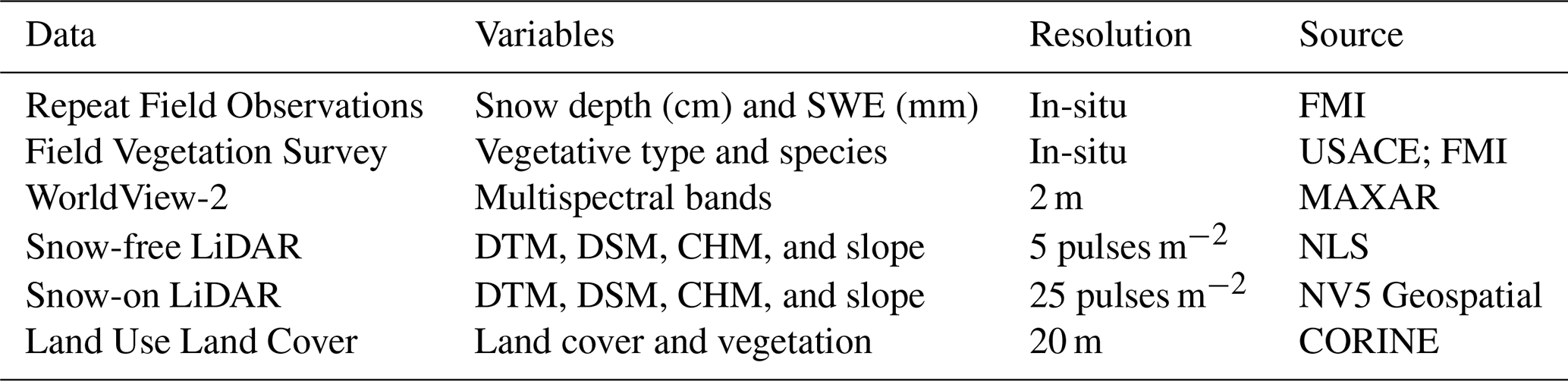
Cloud free and high spatial resolution (2 m) spaceborne WV-2 images from MAXAR were acquired on 2 August 2021 and 27 April 2023. The summer imagery contained spectral readings that matched with distinct vegetative communities, while the winter imagery served to identify snow and non-snow features. Snow-free LiDAR data from 2020 was gathered from the National Land Survey of Finland (NLS) at a density of 5 pulses m⁻². Airborne LiDAR data were obtained on 27 April and 11 May 2023 by NV5 Geospatial and contained full to partial snow cover. This was captured with a Leica City Mapper-2/Hypersion 2+ system containing an average pulse density of ≥25 pulses m⁻², absolute vertical accuracy of ≤6 cm, relative vertical accuracy of ≤15 cm, and horizontal accuracy of ≤14 cm. The LiDAR data were further separated into a Digital Terrain Model (DTM), Digital Surface Model (DSM), and Canopy Height Model (CHM). No major landcover changes impacted the study site during these time periods that would have necessitated the need for repeat sets of imagery.

Land Use Land Cover (LULC) data were acquired from CORINE (Coordination of Information on the Environment) Land Cover (CLC) at 20 m resolution from 2018. CLC is a LULC monitoring program that is coordinated by the European Environment Agency (EEA) and is a current product of the Copernicus Land Monitoring Service (Aune-Lundberg and Strand, 2021). The LULC data was utilized to link vegetative communities to snow depth and SWE in the study area, while excluding artificial features and water bodies. We downscaled the dataset to match the 2 m resolution WV-2 imagery and then updated land cover boundaries where there were evident differences with the obtained summer imagery, thereby providing an updated, higher-resolution LULC. In addition, a modified classification scheme was employed that sought to separate forest communities by soil type and wetlands by moisture content. A RF-based classification scheme was employed for the final land cover predictions and achieved an Overall Accuracy (OA) of 91.7 % and a Kappa value of 0.91, which indicated high LULC classification accuracy. A summary of gathered field and remote sensing variables can be seen in Table 1.

Table 1 Summary of field and remote sensing variables.

3 Methodology

3.1 Image segmentation

An Object-Based Image Analysis (OBIA) technique was utilized to make estimations of snow depth and SWE at the 10 km² local site scale. In OBIA an image is separated into similar groupings of homogeneous pixels known as image objects or segments, which are then utilized as the spatial unit for image assessment (Ye et al., 2018). This contrasts with more traditional pixel-based classification methods, in which image assessment is performed on a pixel-by-pixel basis. The OBIA approach was selected as it has been found to deliver enhanced accuracy and results over traditional pixel-based approaches, especially with high-resolution imagery (Sibaruddin et al., 2018; Shayeganpour et al., 2021; Ez-zahouani et al., 2023). Additionally, outputs generated from traditional pixel-based approaches can be susceptible to high local spatial heterogeneity between adjacent pixels, commonly known as the “salt-and-pepper” effect, which is not evident with OBIA (Wang et al., 2020).

Image segmentation was accomplished with the Segment Mean Shift tool in ArcGIS Pro software, a desktop GIS application. It contains a nonparametric iterative technique that utilizes kernel density estimation to generate image objects from a maximum of three image bands by grouping nearby pixels that contain similar spectral characteristics (Goldberg et al., 2021). The red, green, and near-infrared bands were utilized from the summer WV-2 imagery to carry out image segmentation. For parameters, the spectral detail was set to 19 (near maximum) while spatial detail was set to 1 (minimum) to improve segmentation as both heterogeneous and homogenous areas were present. A total of 37 917 unique image objects were created. Mean and standard deviation were calculated for each image object from the LiDAR and WV-2 datasets. Additional indices utilized included the Green Chlorophyll Index (GCI), Red-Edge Chlorophyll Index (RECI), Normalized Difference Vegetation Index (NDVI), Normalized Difference Water Index (NDWI), and Soil-Adjusted Vegetation Index (SAVI). Descriptions of these widely utilized indices, beyond the scope of this work, are available in Gaitán et al. (2013), Xue and Su (2017), and Nadjla et al. (2022). The automated and field-based snow depth and SWE measurements were spatially joined to polygons with a 3 m radius at each observed field point that each contained average and standard deviation raster band values. This was done to ensure that the input data in this approach better incorporated the spatial context of surrounding features and to improve modeling performance.

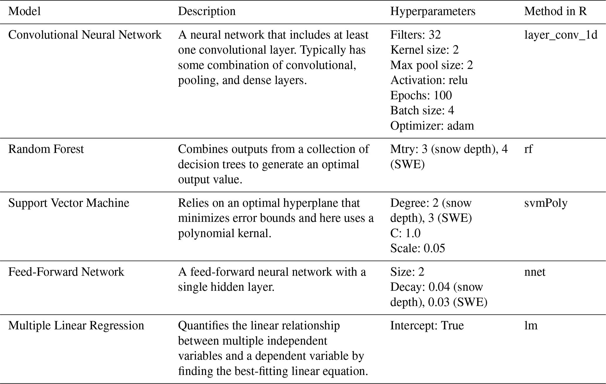
3.2 Machine learning models

In addition to a deep learning Convolutional Neural Network (CNN), other commonly utilized and unique supervised regression-based machine learning models entailing of Random Forest (RF), Support Vector Machine (SVM), Artificial Neural Network (ANN), and Multiple Linear Regression (MLR) were chosen to estimate snow depth and SWE for the image objects. RF works by training a large collection of decision trees to generate an optimal output via bootstrap aggregation (Hwang et al., 2023). In contrast, SVM is a supervised algorithm that relies on an optimal hyperplane that minimizes error bounds and seeks to identify a function that best predicts a continuous output value (Pimentel et al., 2021). ANN may be explained as a feed-forward Directed Acyclic Graph (DAG) connected with artificial neurons with nonlinear activation functions (Li et al., 2022). The architecture of the ANN machine learning model used in this manuscript was a feed-forward network (FFN) model with a single hidden layer. MLR models the linear relationship between independent variables to a dependent variable by finding the best-fitting linear equation (Kim et al., 2020). CNN is a more advanced ANN model that includes at least one convolutional layer (Santry, 2023), though often contains some combination of convolutional layers, pooling layers, and dense layers. Here, a 1D CNN model was utilized as all models relied on the same tabular data provided from all image objects. The tuneGrid parameter found in the caret package in R was used to specify a grid of hyperparameter values for tuning the model training process to optimize machine learning performance. Further details on the hyperparameter values can be found in Appendix A. To aid in reducing potential modeling bias and overfitting, a k-fold cross-validation technique was employed. With this, matched data samples are randomly split into k number of subsets, with k−1 being utilized to train models and the remainder to test models (Abriha et al., 2023). Here, a k-fold of 10 was utilized whereby in each subset 90 % of the data is assigned for training and 10 % is for testing, with model performance determined from the average of all iterations. Thus, each subset of randomly split data is utilized for testing only once, before rejoining the training set. For preprocessing, all inputs were standardized with centering and scaling leading to attributes containing a mean value of 0 and a standard deviation of 1. Subsequently, Principal Component Analysis (PCA) was utilized prior to running each model, which also aided to lessen model overfitting. A threshold of 95 % of the variance captured was set for PCA to ensure that the number of chosen components would sufficiently represent the variance of the data. The result was 17 components for snow depth and 9 components for SWE.

3.3 Object-based ensemble machine learning

An object-based hybrid deep learning and machine learning ensemble approach was applied from a combined weighted output of the CNN, RF, SVM, FFN, and MLR models which is referred to here as Ensemble Analysis (EA). Given that these individual models compute predictions differently and will have varying accuracies and errors, EA can result in a more robust model that considers more accurate models while minimizing the influence of less accurate ones. This is relevant for repeat predictions over the same study site as a model may perform well in one scenario while underperform in another, such as with estimating snow depth during a period of low or high snowfall. All five models were included to estimate snow depth and SWE. The model weights for EA were determined by the coefficient of determination (R²) in which a model with a larger R² value would be given a higher weight, and the sum of weights equal to 1.0 (Zhang et al., 2020). For EA, the weighted average value for each predicted output were calculated by:

$$\begin{array}{}\text{(1)}& \overline{x}={\displaystyle \frac{(x_{\mathrm{1}}\cdot w_{\mathrm{1}})+(x_{\mathrm{2}}\cdot w_{\mathrm{2}})+\mathrm{\dots }+(x_n\cdot w_n)}{w_{\mathrm{1}}+w_{\mathrm{2}}+\mathrm{\dots }+w_n}}\end{array}$$

Where $\overline{x}$ is the weighted average, n is the nth machine learning model, x is the predicted snow depth or SWE value, and w is the weighted model R² value. Combined model uncertainty for EA predictions was based on the standard deviation of model outputs and is referred to as the standard deviation to ensemble prediction (STDE). Other statistical metrics included the Mean Absolute Error (MAE), which is the absolute error between the observed and predicted values, and the Root Mean Square Error (RMSE), which is more sensitive to outliers and is the square root of the mean squared error between observed and predicted values. Larger differences between MAE and RMSE would serve to indicate a high variance of the individual errors from the test samples. Final output metrics were generated from the relationship between actual and estimated outputs. Local scale estimations were generated for snow depth via the ensemble-based approach, which were then utilized as added inputs to aid in upscaling the more limited field acquired SWE data to the same local scale. Snow density was measured by dividing the estimated SWE by the estimated snow depth in each respective instance. A summary of the methodology framework can be found in Fig. 3. Image objects were generated from multispectral imagery via image segmentation, with averaged remote sensing and field snow depth values assigned to each unique image object (1). Standardization and PCA were applied to the spatially matched data before then being evaluated through the base machine learning models (CNN, RF, SVM, FFN, and MLR) to predict snow depth before being ascertained with EA by combining model outputs with weighted averaging based on the R² value of each model (2). Model metrics were obtained from each model alongside the mapped estimated local scale snow depth, with the estimated snow depth from EA and field SWE values then being spatially joined to the previously matched input data (3). Standardization and PCA were again applied to the updated spatially matched data and was analyzed by the same base machine learning models (CNN, RF, SVM, FFN, and MLR) to predict SWE before being finalized with EA (4). Model metrics were generated along with the mapped estimated local scale SWE in each instance (5).

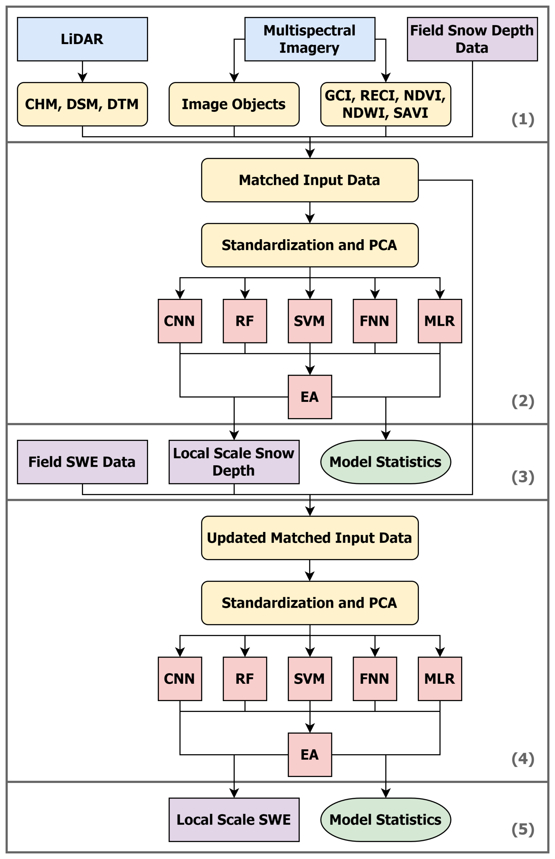
Figure 3 Methodology framework to upscale field snow depth data to a local scale by using an object-based ensemble machine learning approach and then joining the produced snow depth outputs and matched input data with the field SWE data to generate local scale SWE outputs. Blue indicates input data, purple indicates outcome variables, yellow indicates processed data, red indicates machine learning, and green indicates model metrics. CNN is Convolutional Neural Network, RF is Random Forest, SVM is Support Vector Machine, FFN is Feed-Forward Network, MLR is Multiple Linear Regression, and EA is Ensemble Analysis.

While the methodology is similar to that found in Brodylo et al. (2024), that work was solely intent on upscaling 1 m² permafrost active layer thickness (ALT) field data to three 1 km² local scale sites in Alaska before then further upscaling the ALT estimates to a 100 km² regional scale over multiple years. Here, we focused on first upscaling repeat field snow depth measurements to a 10 km² local scale in Finland over multiple instances with a novel object-based hybrid deep learning and machine learning ensemble approach and then combined the estimated snow depth data to the original machine learning input data. The addition of snow depth as an input variable enabled a separate, enhanced estimate of SWE at the same 10 km² local scale with more limited repeat field SWE measurements over the same multiple instances in a single winter period. This then permitted snow density to be calculated at each moment in time from snow depth and SWE estimations. The approach was applied to a shorter temporal analysis for snow depth, SWE, and snow density. It revealed how each of these variables were interconnected during the initial, middle, and late winter, how machine learning models performed over the course of the winter period, and how the studied variables related to landcover types over these different instances. In addition, machine learning snow depth estimates were directly compared to independent LiDAR-based snow depth estimation.

4 Results

4.1 Snow depth

All tested models performed relatively well with the snow depth estimations. The best R², MAE, and RMSE values were observed with RF, SVM, FFN, and EA (Fig. 4). Owing to the lower snow depth in December, MAE and RMSE were the smallest out of all six instances at 1.7 and 2.4 cm for EA, respectively. MAE and RMSE steadily increased for all models from roughly 1.5–2.7 and 2.0–3.4 cm in December to 4.5–6.1 and 5.1–8.1 cm at the end of April. This was expected given increased snowfall and snow depth over time, alongside minor periods of snowmelt throughout and accelerated snowmelt in April that would increase model uncertainty. The R² value for EA was strongest during peak snow depth in March (0.92), while being somewhat lowered in December (0.79) during the lowest observed snow depth. RF and EA tended to have the most consistent and best or second best R², MAE, and RMSE values across all six instances. This was in contrast with metrics produced from CNN, SVM, FFN, and MLR. CNN contained metrics that were relatively in-line with other models in the first and second instances. However, during the last four instances there was a more noticeable drop in metric performance. SVM and FFN performed well and were able to match or exceed RF and EA in several instances, though never generated the highest R² values. MLR lagged in metric performance to most models, yet it still provided respectable metric values. More information about outputs produced with EA for each instance can be seen in Fig. 5, with each instance containing a 1:1 line, fitted linear regression line, and scatterplot with STDE error bars in blue. With minor exceptions, there was largely an overall agreement between the field and estimated snow depth values, and between the individual model outputs.

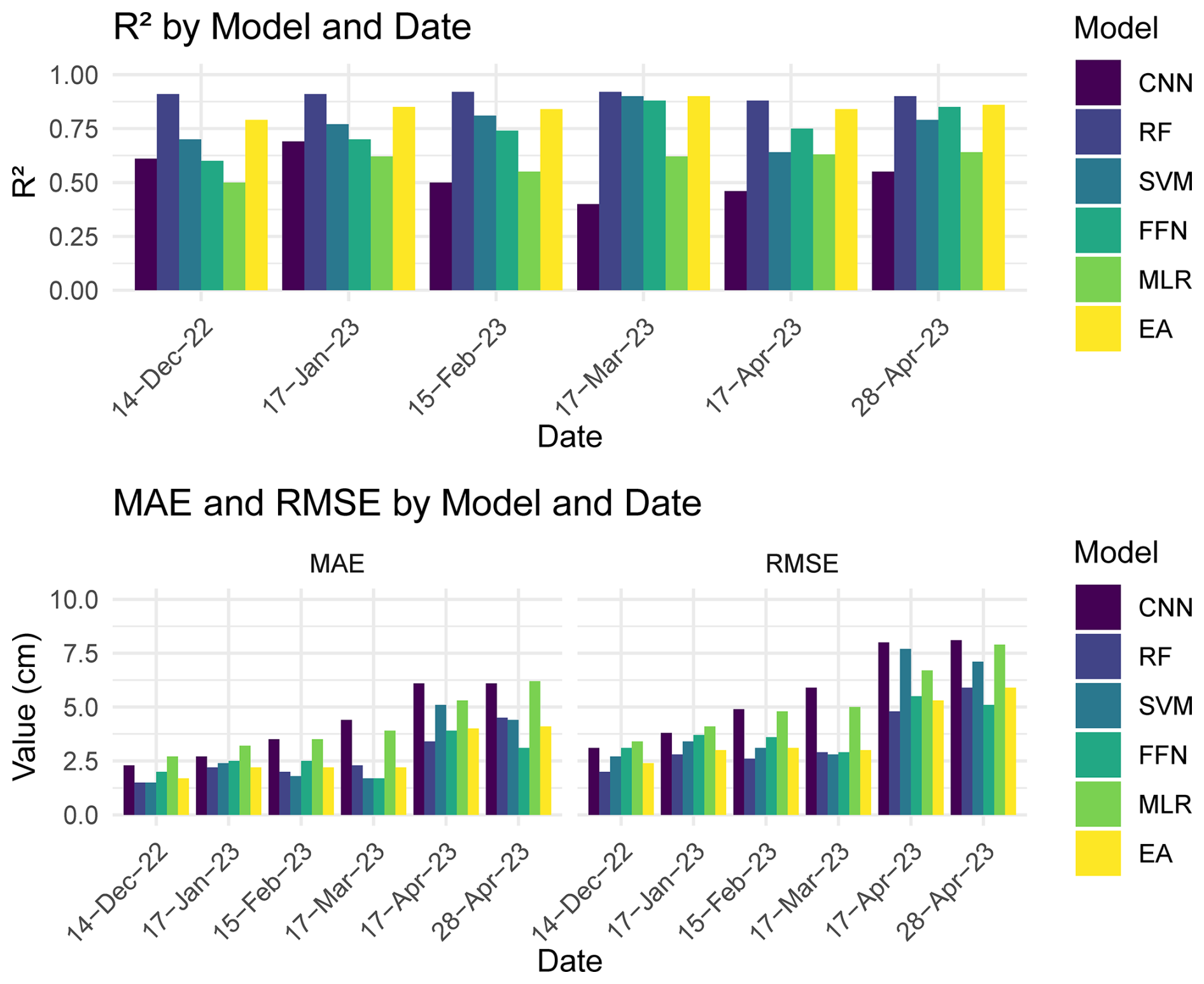
Figure 4 Machine learning model metrics for estimated snow depth with CNN, RF, SVM, FFN, MLR, and EA. MAE and RMSE are in cm.

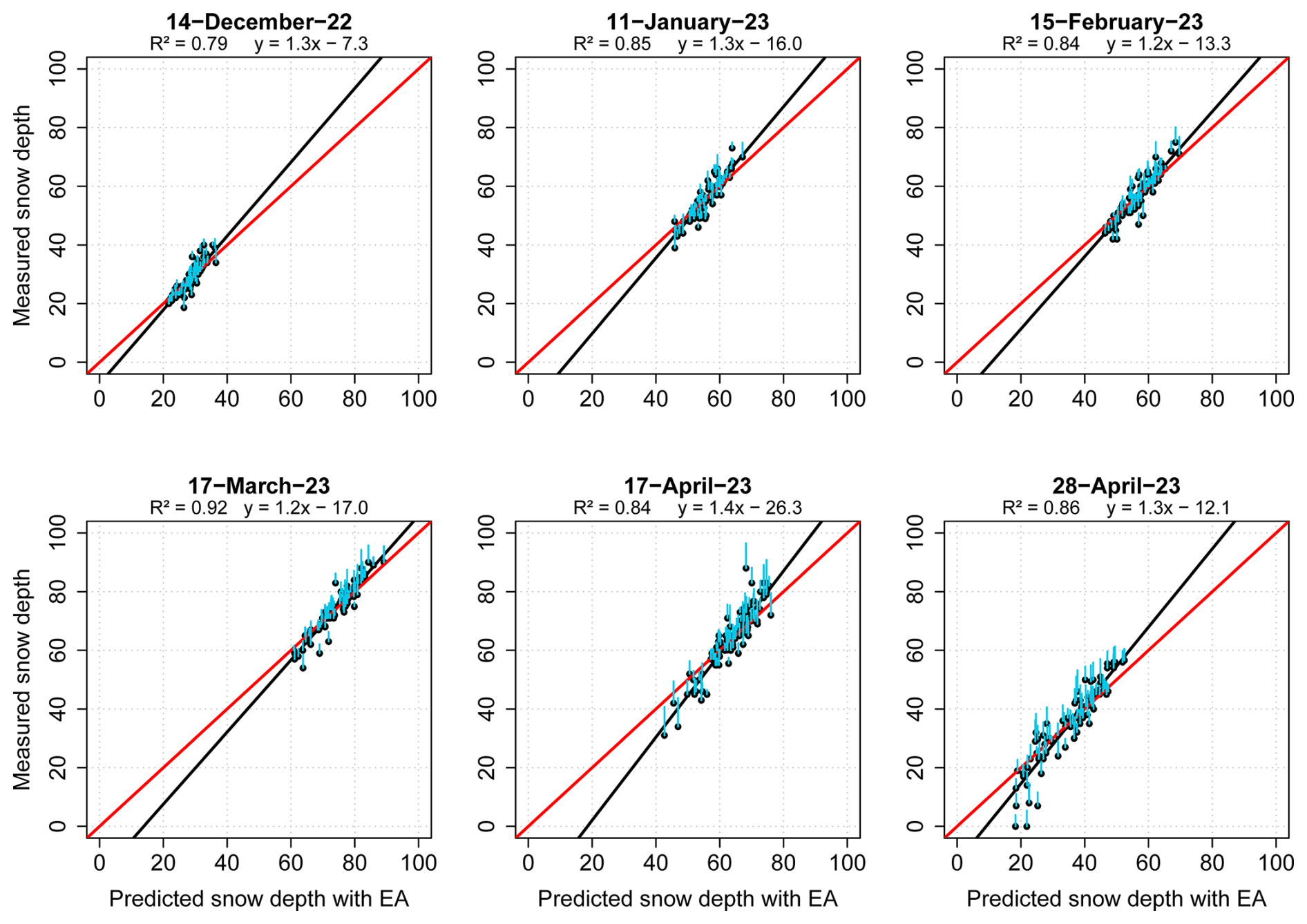
Figure 5 Scatterplot, 1:1 line (red line), and fitted regression line (black line) between the predicted snow depth from EA and the measured snow depth on each occasion from 14 December 2022 until 28 April 2023. STDE is in cyan.

The snow depth average and standard deviation at each of the vegetative land cover types with the field data and local scale EA outputs are in Fig. 6. Mapped snow depth at the field scale and local scale estimates with EA for each instance from December 2022–April 2023 can be seen in Fig. 7. There was a general agreement and similar snow depth patterns in LULC's that contained both field and local scale data. The average snow depth was lowest for the field data at 29 cm and local scale at 32 cm in December, while the highest readings were in March at 75 and 80 cm, with a rapid decline at the end of April at 36 and 40 cm. Standard deviation was lowest in December (±5 and ±4 cm) for both while highest at the end of April (±13 and ±9 cm) when there was increased snowmelt. At the field scale there was up to a 10–11 cm difference between coniferous forest (peat soil) and coniferous forest (mineral soil) from January to early April. The exception is at the end of April during the period of snowmelt when field coniferous forest (mineral soil) contained higher snow depth at 43 cm than coniferous forest (peat soil) at 40 cm. A similar pattern was evident with the field transitional woodland/shrub (peat soil) repeatedly containing higher snow depths than transitional woodland/shrub (mineral soil) with a maximum difference of 10 cm in early April. However, at the end of April both were equal at 36 cm of snow depth. Field-based peatbog (wet) and open area contained the lowest levels of snow depth in all instances, ranging from 26–70 and 25–70 cm, respectively, with the latter experiencing elevated standard deviation of ±20 and ±22 cm in the last two instances.

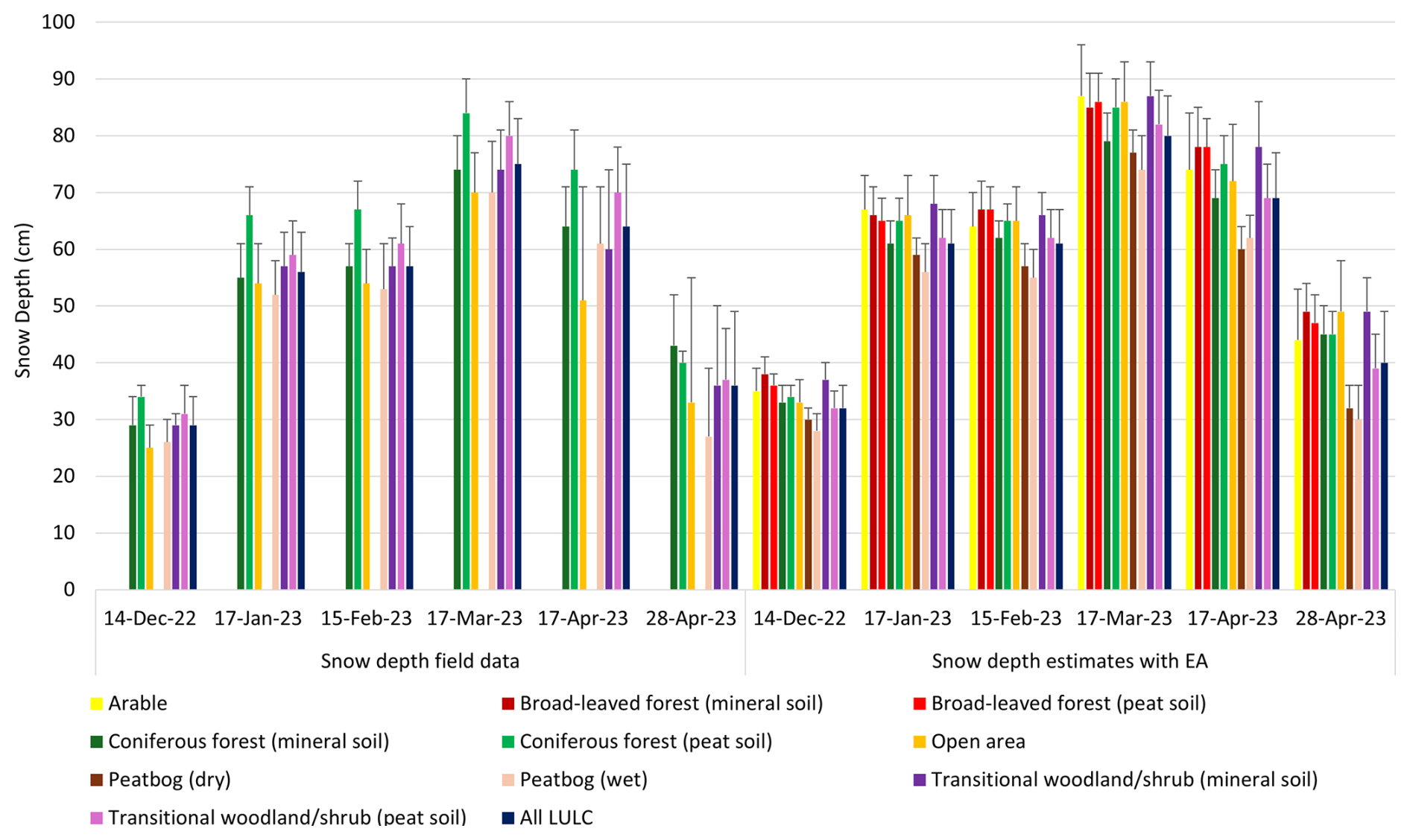
Figure 6 Mean and standard deviation (error bars) for snow depth (cm) estimates per LULC with field data and at the local scale with EA. Blank values indicate no field data.

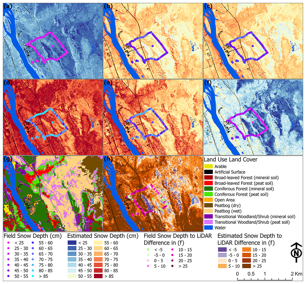
Figure 7 Field and estimated snow depth (cm) in (a) 14 December 2022, (b) 17 January 2023, (c) 15 February 2023, (d) 17 March 2023, (e) 17 April 2023, and (f) 28 April 2023 alongside (g) a LULC map and (h) 28 April 2023 snow depth difference from 27 April 2023 collected LiDAR.

At peak snow depth at the local scale in March, both dry and wet peatbogs contained the lowest average snow depth at 77 and 74 cm, alongside having the lowest snow depths in all other instances, particularly for wet peatbogs. Dry, unsaturated peatbog was found to have snow depths greater than wet, saturated peatbog, with differences ranging from 2 to 3 cm, apart from early April when wet, saturated peatbog had 2 cm more snow depth. Arable and open area contained similar estimated snow depth values in all instances except in the end of April with a 5 cm difference and were higher than dry and wet peatbogs from December to the end of April. Forests and transitional woodlands largely contained the higher average values in March with broad-leaved forest recording 85 cm (mineral soil) and 86 cm (peat soil), coniferous forest (peat soil) with 85 cm, and transitional woodland/shrub containing 87 cm (mineral soil). There was also a consistent 0–2 cm snow depth difference between the local scale broad-leaved forest mineral soils and peat soils, with a slight reversal of 1 cm in March. Transitional woodland/shrub contained higher snow depth in mineral soil than in peat soil in all instances despite the field data having the opposite pattern, which may be due to certain terrain and vegetative factors being higher prioritized in model performance for areas further away from gathered field observations. Local scale coniferous forest (peat soil) consistently contained snow depth values greater than coniferous forest (mineral soil), with up to a 6 cm difference from December to early April. At the end of April both had the same average snow depth of 45 cm. In addition, field and local scale snow depth estimates from 28 April were compared to the difference between snow covered DTM from the prior day and snow-free DTM from 2020. Results indicate field snow depth measurements generally exceeded the estimated LiDAR-based snow depth estimations by an average of 9.6 cm, while for the local scale with EA it was higher at 13.1 cm.

4.2 Snow water equivalent

Machine learning model performance for SWE estimation between CNN, RF, SVM, FFN, MLR, and EA can be seen in Fig. 8. Given more limited field-based SWE measurements with 13 samples, the models would have encountered more pronounced challenges matching estimations to real-world data yet were generally able to produce acceptable results in part due to the inclusion of snow depth data. FFN and EA largely contained the most stable and positive metrics for R² in most instances. SVM, FFN, and EA generally produced the best overall metrics, although MLR was able to provide the second-best metrics in some instances for MAE and RMSE. Metrics from CNN were somewhat on-par with other models in December and end of April though it had poor performance between January and early April. SVM varied to a lesser extent, with it being on-par with models in most instances except with poorer overall metrics in February and March, along with notably high MAE and RMSE values at the end of April. While the best base model performance for EA inputs was RF, SVM, and FFN over different instances for snow depth, for SWE it was largely from FFN and MLR, and to a lesser extent RF and SVM in different instances. In both cases, EA was able to provide positive metrics and never poor metrics. A scatterplot, 1:1 line, and fitted linear regression line for each instance of SWE predictions produced by EA alongside STDE can be seen in Fig. 9. Similarly with the snow depth metrics over the same period, MAE and RMSE were lowest in December from roughly 0.4–2.9 and 1.0–4.6 mm before rising to become the highest at the end of April at 7.0–32.0 and 10.0–39.0 mm.

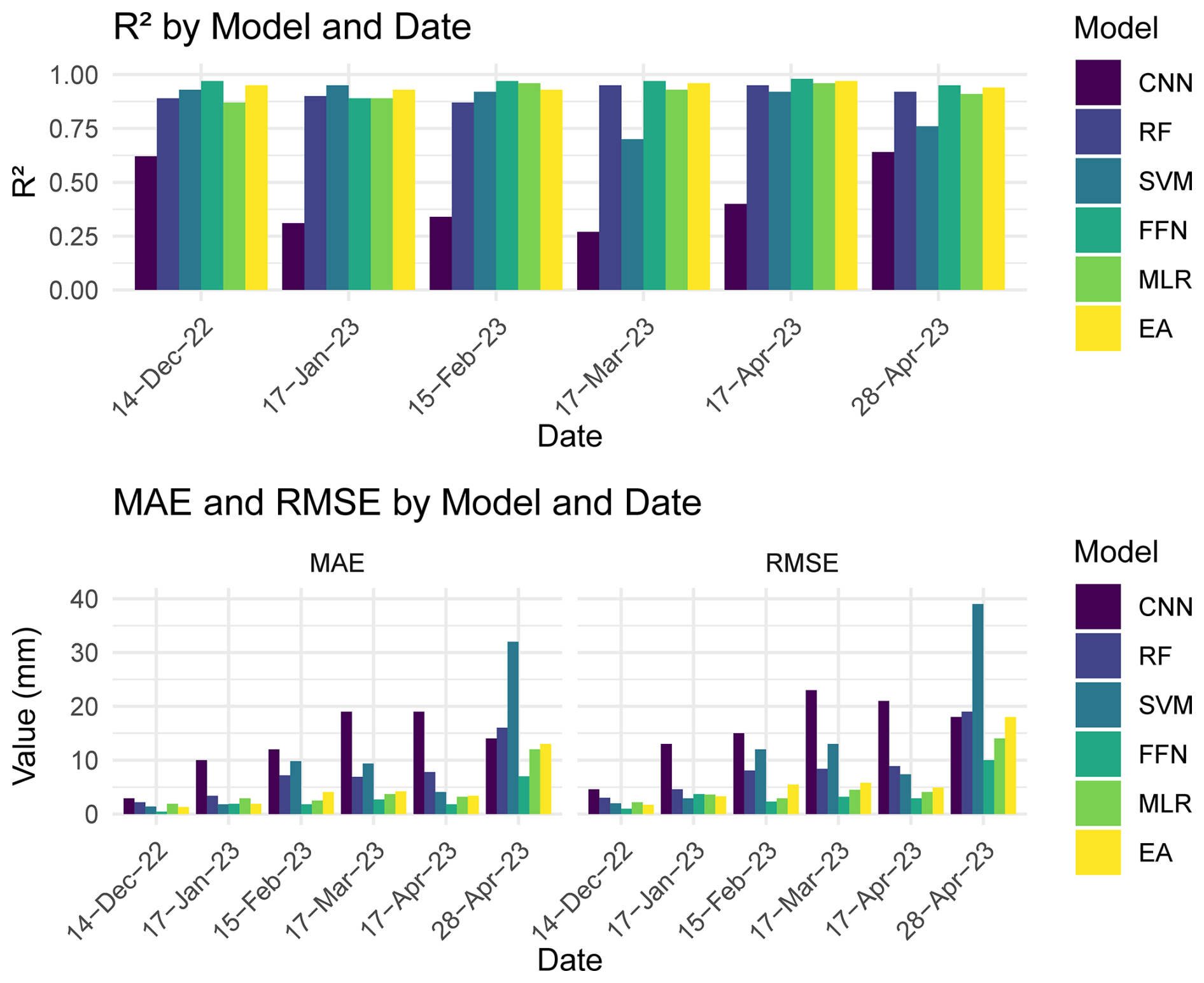
Figure 8 Machine learning model metrics for estimated snow water equivalent with CNN, RF, SVM, FFN, MLR, and EA. MAE and RMSE are in mm.

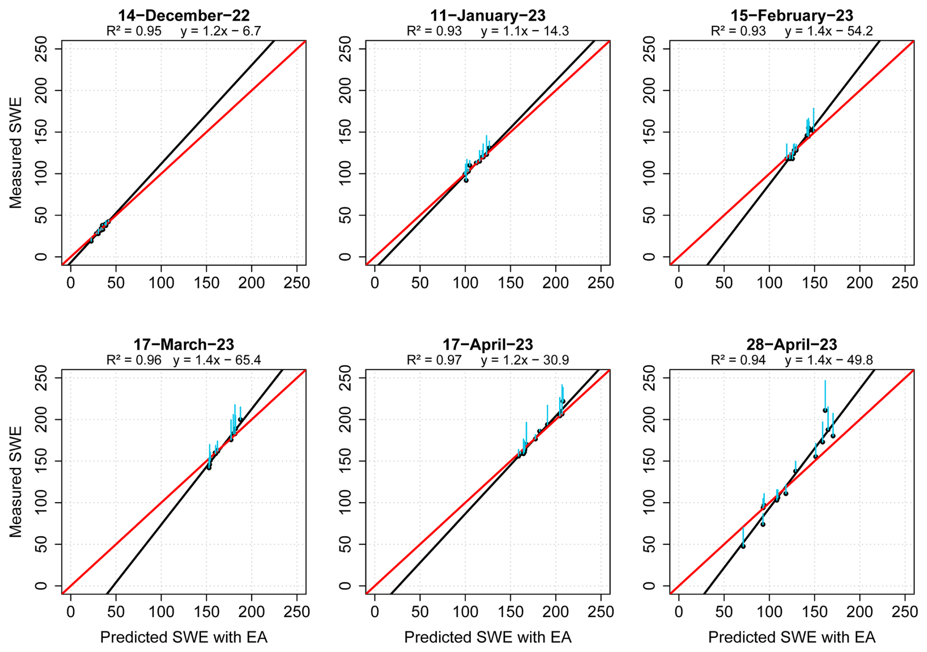
Figure 9 Scatterplot, 1:1 line (red line), and fitted regression line (black line) between the predicted SWE from EA and the measured SWE on each occasion from 14 December 2022 until 28 April 2023. STDE is in cyan.

The average and standard deviation of SWE field data and local scale EA outputs at the vegetative land cover types for all instances can be seen in Fig. 10. A distribution of SWE over the 10 km² site for each instance from December 2022–April 2023 can be seen in Fig. 11, which illustrates where and how much SWE varied over time for the field data and EA-based local scale outputs. SWE maximums occurred in early April and were after peak snow depth in March. With the field data, the average SWE was lowest at 34 mm in December and then peaking at 177 mm in early April before dropping to 131 mm in late April. A similar pattern was evident with the local scale average SWE outputs with 37 mm in December that later peaked at 184 mm in early April before dropping to 133 mm at the end of April. From the field data, coniferous forest (mineral soil) largely had the lowest SWE values from December (30 mm) to early April (173 mm). This was in sharp contrast to transitional woodland/shrub (peat soil) which had the highest SWE values during that same period from 38 to 183 mm before dropping sharply to 119 mm at the end of April. Open area tended to have higher SWE values, while peatbog (wet) gravitated to lower SWE values. Largely corresponding to the SWE quantity and time, standard deviation was lowest in December ranging from ±3 to ±9 mm while highest at the end of April between ±34 to ±80 mm.

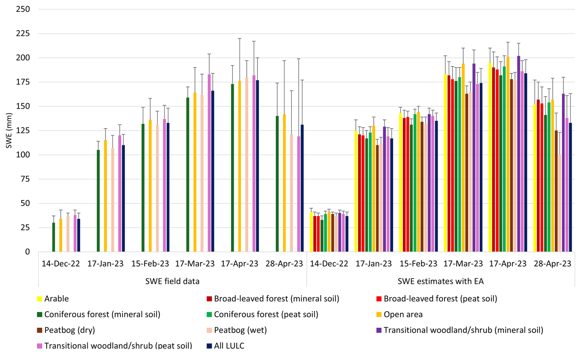
Figure 10 Mean and standard deviation (error bars) for SWE (mm) estimates per LULC with field data and at the local scale with EA. Blank values indicate no field data.

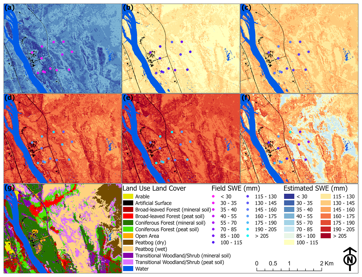
Figure 11 Field and estimated SWE (mm) in (a) 14 December 2022, (b) 17 January 2023, (c) 15 February 2023, (d) 17 March 2023, (e) 17 April 2023, and (f) 28 April 2023 alongside (g) a LULC map.

At the local scale, the landcover types with the highest SWE values in all instances were arable, open area, and transitional woodland/shrub (mineral soil). These areas were similar in that they contained little to no inundated land along with a lack of bushes and trees. The highest SWE values were in early April for all three landcover types at 195, 201, and 202 mm respectively. The lowest SWE values in all instances tended to be found in coniferous forest (mineral soil), peatbog (dry), peatbog (wet), and transitional woodland/shrub (peat soil). Peatbog (wet) contained some of the lowest SWE values from January (111 mm) to the end of April (100 mm), which was somewhat in contrast to peatbog (dry) during the same period from 110 mm in January to 125 mm at the end of April. SWE values for broad-leaved forest in mineral and peat soil tended be similar and slightly above average, while there was greater variation for coniferous forest. Coniferous forest (mineral soil) consistently contained lower SWE values than did coniferous forest (peat soil) with differences between 2 to 12 mm. Transitional woodland/shrub (mineral soil) also repeatedly had higher SWE values than transitional woodland/shrub (peat soil) in all instances, with differences varying from 1 to 25 mm. The standard deviation values for the EA values were less volatile than with the field data, with it ranging from 4 mm in December to 30 mm at the end of April.

4.3 Snow density

Snow density is the ratio between the volume of water produced by melting a given volume of snow and the original volume of snow itself. This percentage refers to the water content within a given volume of snow. In general, fresh snowfall has low density while older, compacted, or wind-effected snow will have a higher density. Figure 12 contains the mean and standard deviation of the snow density percentage for each vegetative landcover type from December to the end of April. The average snow density percentage for field and local scale data was lowest in December with 12 % for both, while the highest was at the end of April at 36 % and 34 %, respectively. Standard deviation for the combined averages were generally low, with a maximum of ±4 % in late April for both field and local scale EA estimates. While the field standard deviation for specific landcover types could increase to ±3 % prior to early April, for the local scale EA estimates it only reached ±2 % for open area once during that same period. For the first five instances the field snow density percentages were slightly higher with the canopy-free open area and peatbog (wet), which ranged from 14 %–31 % and 13 %–29 %. In contrast, the more tree-covered coniferous forest (mineral soil) and transitional woodland/shrub (peat soil) routinely experienced lower percentages ranging from 11 %–27 % and 13 %–27 %. In the final instance, field transitional woodland/shrub (peat soil) and peatbog (wet) had the highest snow density percentages at 42 % and 39 %, while open area and coniferous forest (mineral soil) were markedly lower at 33 % and 32 %.

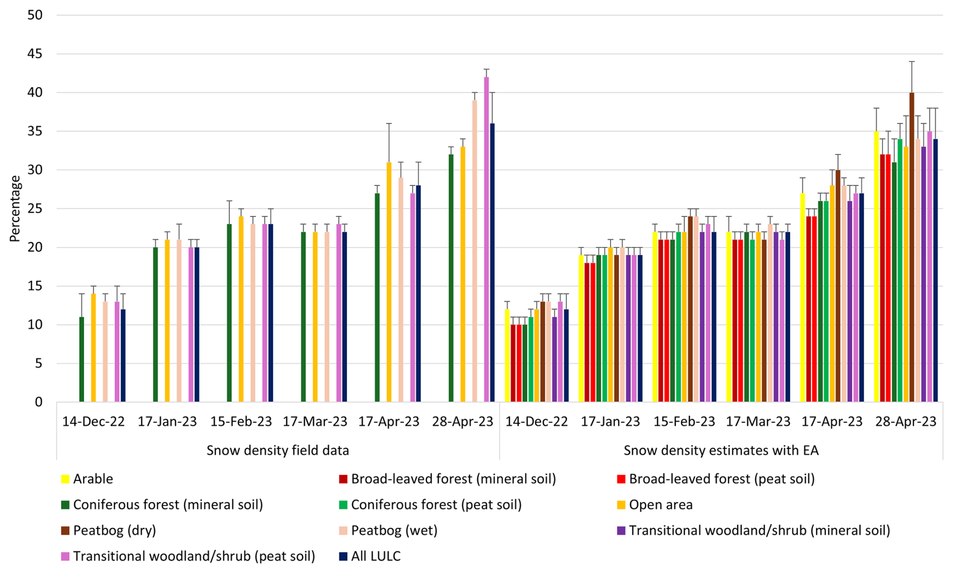
Figure 12 Mean and standard deviation (error bars) for snow density percentage estimates per LULC with field data and EA. Blank values indicate no field data.

As with the field averages, for the local scale averages from December to early April there were generally minimal differences in snow density between different land cover types while experiencing greater fluctuations at the end of April with a maximum difference of 9 %. The highest snow densities were generally found with open area and more so with peatbog (wet) and peatbog (dry). Peatbog (wet) contained percentages equal or up to 2 % higher than peatbog (dry) from December to March. However, in both early and end of April it reversed with peatbog (dry) containing higher snow densities at 30 % and 40 % compared to peatbog (wet) at 28 % and 34 %. The lowest values were generally found with broad-leaved forest (mineral soil) and broad-leaved forest (peat soil), which always differed by less than 1 %. Coniferous forest (mineral soil) and coniferous forest (peat soil) also tended to have similar values. However, by late April the snow density in coniferous forest (peat soil) was 3 % higher during that period of rapid snow melt, with coniferous forest (mineral soil) having the lowest snow density at 31 %. Average snow density percentage on transitional woodland/shrub (mineral soil) and transitional woodland/shrub (peat soil) were similar with a maximum difference of 2 %. A spatial view of the gradual increase in the snow density percentage across the six instances with the rapid rise at the end of April can be seen in Fig. 13.

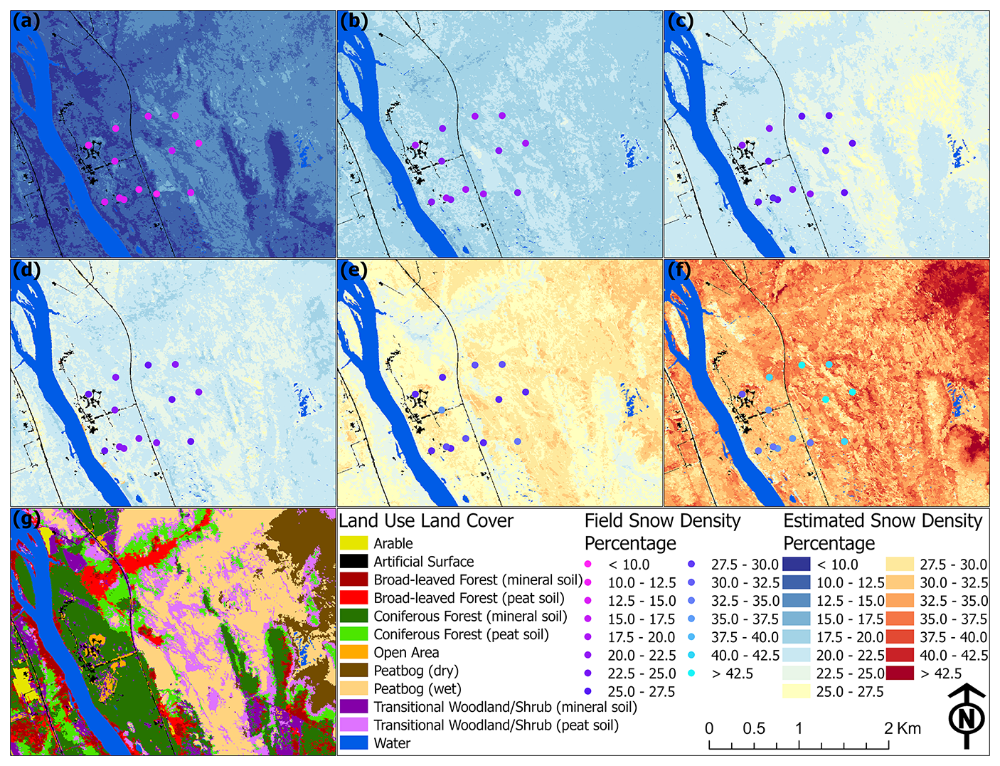
Figure 13 Field and estimated snow density percentage in (a) 14 December 2022, (b) 17 January 2023, (c) 15 February 2023, (d) 17 March 2023, (e) 17 April 2023, and (f) 28 April 2023 alongside (g) a LULC map.

5 Discussion

With snow depth estimation, all models performed well, with RF, SVM, FFN, and EA particularly being capable of generating encouraging statistics. As is common for the study region the snow depth was lowest in December and highest in March before daily temperatures began exceeding 0 °C in April. There were consistent differences in snow depth between different vegetative communities. This was most apparent with higher snow depth being associated with broad-leaved forests, transitional woodland/shrubs, and particularly with coniferous forest (peat soil). Shallower snow depth was recorded at coniferous forest (mineral soil), open areas, and both dry and wet peatbogs. With peatbogs, wet peat conducts heat better than dry peat resulting in heat flowing more effortlessly in wet peat layers in winter (Kujala et al., 2008), which may result in increased snowmelt and compaction. Furthermore, mineral soil is more thermally conductive than peat soil (Atchley et al., 2016), which may promote snowmelt and compaction in similar vegetation communities containing mineral soil compared with peat soil where snowmelt and compaction would be reduced. Forests with drier mineral soils were generally more shielded from saturated soil found in peatbogs, while forests with peat soil were oftentimes adjacent to peatbogs. As the water table in many parts was at or near the surface, adjacent soils would contain greater soil saturation while the shielded mineral soils would in theory be more unsaturated. A notable exception is for approximately half of the broad-leaved forest (mineral soil) that is along the Kitinen River, which may have especially influenced snow depth, SWE, and snow density readings for that LULC. Given that saturated soil needs greater energy to heat than does unsaturated soil (Howe and Smith, 2021), saturated soil would require greater energy to warm in the spring and remain warmer in the winter than the unsaturated soil, which would have a resulting impact on snow cover. Post winter soil thaw varied with five FMI Campbell Scientific 109-L soil temperature sensors in the study area at 5 and 10 cm below the surface. For two sensors found in coniferous forest and one in an open area with mineral soil, the soil fully thawed out between 10–25 April, while for the two sensors in the peatland, the soil thawed out from 11–13 May, which would have aided in accelerating overlaying snow cover melt for the former. It should be noted the impact that direct solar radiation may have on the energy balance of the snowpack and melt processes, along with wind impacted (open areas) versus wind protected (forest) vegetative communities. Lastly, snow interception and sublimation are major factors in forest communities, especially with conifers, which can lead to a notable diversity of snow accumulation on the forest floor (Helbig et al., 2020).

For the SWE estimations, model results were more mixed, but nonetheless promising. RF, SVM, FFN, and EA were all able to produce positive metrics, while there was elevated variation with both CNN and to a lesser extent SVM. MLR also performed well despite being the simplest form of machine learning in this study. While the higher snow depth sample size may have benefited more complex models for snow depth modeling, simpler models seemed to perform better with the more limited SWE sample size. A greater number of SWE field samples would have provided enhanced findings; however, these field measurements can be time-consuming and expensive to collect across a large geographic region, with SWE measurements taking approximately 20 times as long to complete compared to snow depth measurements (Sturm et al., 2010). Nonetheless SWE was found to be lowest in December and highest in early April, which was post-peak snow depth. With the field data, it was found that SWE was higher in transitional woodland/shrub (peat soil) than with coniferous forest (mineral soil), which may be attributed to potentially more saturated peat soil allowing for greater water retention within the snow cover, while the unsaturated mineral soil drained slightly more liquid from the overlaying snow cover. Mineral soils across the study site are sand-rich and would be dry most of the time at the surface and likely never reach saturation, with any melted snow being drained in these soils. The one exception was with the end of April when there was a notable reversal, which may have been due to increased snow interception, snowmelt, sublimation, and windblown snow from branches in some vegetation types. A similar trend was observed at the local scale. Local scale coniferous forest (peat soil) continually contained higher average SWE than coniferous forest (mineral soil) which may be the result of the unsaturated mineral soil absorbing water from the overlaying snow while the saturated peat soil slowed the draining of water through the snowpack and into the soils. Dry and especially wet peatbogs largely contained the lowest SWE measurements. These low open areas likely experienced enhanced wind activity that blew snow laterally away while also leading to greater sublimation. This would have led to greater snow particle cohesion and denser wind slab layer formation at the surface of the snowpack due to sintering after snow was mobilized in the wind (Mott et al., 2018).

Lastly, snow density was lowest in December and increased until the end of April when it was highest, which was during a period of rapid snowmelt. This was to be expected given that the beginning and middle winter typically contain larger quantities of fresh snowfall, while by the end of winter the snowpack would have compacted over time and become denser as the snowpack reaches an equilibrium temperature state of 0 °C (e.g., isothermal). As the snowpack develops, a larger snow grain size (depth hoar) results in a lower density in shallow snowpack. However, as the snowpack becomes isothermal, the depth hoar layer will metamorphose and become denser, especially near the ground (Gu et al., 2019). With the field data, a higher snow density percentage was observed at the end of April in peatbog (wet) and transitional woodland/shrub (peat soil) which contrasted with coniferous forest (mineral soil) and open area and may be attributed to soil saturation for those specific locations. At the end of April for the local scale the highest snow density percentages were found in vegetative communities that were more impacted by wind such as arable along with peatbog (wet) and peatbog (dry). In contrast, both broad-leaved forest and coniferous forest in mineral and peat soils typically had the lowest percentages. Local scale wet peatbog was found to generally contain slightly higher amounts than dry peatbog. This may be attributed to dry peatbog being on average ∼2.2 m higher in elevation than wet peatbog in our study area, which may have contributed to the movement of water over time to wet peatbogs at incrementally lower elevations.

Solar radiation increased throughout the timeframe and was not uniform over the study area, such as with thick forests sometimes obscuring adjacent canopy-free areas from solar radiation. As this would have impacted real-world snow estimates, we incorporated end of winter WV-2 imagery in the framework as it was able to aid in capturing such irregularities. A limited quantity and spatial extent of field measurements restricted further associations with vegetative communities, especially for SWE and, in turn, snow density. Had additional measurements been taken at communities missing field data, there would be a more comprehensive understanding of snow-landcover relationships. Additional datasets would have likely improved the model statistics and estimation of all three studied features. Soil moisture and air/subsurface temperature data were accessible in the study area yet were excluded, despite their strong association with snow depth and SWE (Contosta et al., 2016). This was due to a limited number of these measurements that corresponded to the six instances, with some containing gaps or missing data which would hinder spatial mapping and association with landcover types. Furthermore, very few of these measurements were located on or adjacent to the field snow depth and SWE measurements, which severely limited a proper linkage between the field data with soil moisture and temperature. Additional remote sensing-based data could have been utilized as an add-on to assist in mapping soil moisture and temperature for the study, alongside improving estimations for snow depth and SWE. However, due to the vegetative heterogeneity at the 10 km² site and clustering of the field data, medium and low-resolution imagery would have provided questionable benefit. High-resolution hyperspectral imagery and Synthetic Aperture Radar (SAR) are particularly relevant, given the additional available spectral bands of the former and the proven application with snow depth and SWE detection in the latter (Patil et al., 2020) and would have likely benefited the findings.

The applied model was able to establish connections between remote sensing data and snow measurements to estimate surrounding snow depth, SWE, and snow density over multiple instances. In terms of performance, it was seen with the more numerous field snow depth data that more complex machine learning and a deep learning model could perform well, while in instances of very limited data for SWE, simpler models were more prone to succeed. Regardless of the sample size, an ensemble approach of different models was able to perform well in both circumstances whereby it can adapt its effectiveness in the case of changing the output variable and sample size. In terms of model transferability from this effort, in conditions where there are plentiful input data for model training, more complex deep learning and machine learning models should be utilized to better identify intricate patterns. However, with a more limited training sample size it would be imperative to ensure that the gathered data is of high quality and covers differing topographic and vegetative features to aid with model predictions over an area. This added flexibility in the types of base models to be used for such an ensemble approach allows it to be applied to smaller snow-related datasets covering local scale areas, to larger datasets with hundreds or thousands of data points that can cover regional and potentially global scales. In any case, model inputs would need to be appropriately defined regarding the type of terrain and data to be utilized, such as for example field data along mountain ranges compared to low-lying open areas.

6 Conclusions

We employed an object-based hybrid deep learning and machine learning ensemble approach with time-series field snow depth and SWE data in northern Finland to first estimate snow depth at a local scale, before incorporating the snow depth outputs to estimate SWE at the same local scale alongside generating snow density estimations from six instances between December 2022 and April 2023. Snow depth peaked in March, SWE peaked shortly after in early April, and snow density peaked with the final available data at the end of April. Multiple machine learning models, particularly with the ensemble approach, were shown to positively estimate key snowpack attributes over the period at the study site in Sodankylä despite limited field snow depth and SWE observations. We established that there are direct spatial and temporal connections between three commonly studied snowpack elements with vegetation and soil types, with more research recommended to further characterize these associations. Although there is promise with intricate deep learning and machine learning techniques, this study also highlights opportunities to assess where less complex methods may be employed for computational efficiency and performance, especially when scaling up. While performed over a small portion of northern Finland, when matched with other field-based snowpack and remote sensing data across the region it would be possible to further upscale the studied snow-based estimates over a wider, regional-scale over various periods in time. This would also need to account for differing types of snowpack, terrain, and vegetative communities found throughout the pan-Arctic domain. As average temperatures around the Arctic are projected to increase with fewer days below freezing, more uncertain climactic conditions and precipitation events would affect the quantity, rate, and timing of snowfall, snow-on/snow-off, and snowmelt runoff in the region. Given that waterbodies such as lakes, ponds, and rivers in Finland and other high latitude areas are fed by the annual snowmelt, any changes to this natural process would meaningfully alter the hydrological makeup. The hybrid-based methodology applied in this effort can serve to benefit future snow-related analyses in high latitude regions, alongside other areas on Earth that regularly experience seasonal snow.

Appendix A

In this appendix, we present relevant model hyperparameters utilized in the study. Model parameters remained the same during each of the six instances to ensure fair comparisons, with the best optimization values being automatically selected.

Table A1 List of model summaries and hyperparameters.