The Greenland-Ice-Sheet evolution over the last 24 000 years: insights from model simulations evaluated against ice-extent markers

Continental ice sheets retain a long-term memory stored in their geometry and thermal properties. In Greenland, this creates a disequilibrium with the present climate, as the ice sheet is still adjusting to past changes that occurred over millennial timescales. Data-consistent modelling of the paleo Greenland-Ice-Sheet evolution is thus important for improving model initialisation in future projection experiments. Open questions also remain regarding the ice sheet's former volume, extent, flux, internal flow dynamics, thermal conditions, and how such properties varied in space since the last glaciation. Here, we conduct a modelling experiment that aims to produce simulations in agreement with empirical data on Greenland's ice-margin extent and timing over the last 24 000 years. Given uncertainties in model parameterisations, we apply an ensemble of 100 ice-sheet-wide simulations at 5×5 km resolution using the Parallel Ice Sheet Model, forced by simulations from the isotope-enabled Community Earth System Model. Using a new Greenland-wide reconstruction of former ice margin retreat (PaleoGrIS 1.0), we score each simulation's fit from 24 000 years ago to 1850 AD. The results provide insights into the dynamics, drivers, and spatial heterogeneities of the local Last Glacial Maximum, Late-glacial, and Holocene evolution of the Greenland Ice Sheet. For instance, we find that between 16 and 14 thousand years ago, the ice sheet lost most ice grounded on the continental shelf. This marine-sector retreat, associated with mass loss rates up to seven times greater than today's, was likely mainly driven by ocean warming. Our model–data comparison results also show regional heterogeneities in fit and allows estimating agreement-score sensitivity to parameter configurations, which should prove useful for future paleo-ice-sheet modelling studies. Finally, we report remaining model-data misfits in ice extent, here found to be largest in northern, northeastern, and central-eastern Greenland, and discuss possible causes for these.

1 Introduction

Due to anthropogenic climate change, the Greenland Ice Sheet (GrIS) is losing mass at an increasing rate and is now a major contributor to global mean sea-level rise (Meredith et al., 2019). Its future contribution remains uncertain, with projections showing large discrepancies, most ranging between ∼ 70 and ∼ 190 mm of sea-level rise by 2100 under the RCP 8.5/SSP5-85 scenarios (Aschwanden et al., 2019; The IMBIE Team, 2019; Goelzer et al., 2020; Edwards et al., 2021). Reducing uncertainties in GrIS projections is crucial not only for estimating sea-level rise and Greenland-wide changes, but also for anticipating broader climate impacts, partly due to the ice sheet's influence on ocean circulation and the potential slowdown of the Atlantic Meridional Overturning Circulation (AMOC) from increased freshwater release (Yu et al., 2016; Martin et al., 2022; Sinet et al., 2023). A major source of uncertainty relates to model initialisation, i.e. the “spinup” required to set an appropriate initial state (Rogozhina et al., 2011; Seroussi et al., 2019). This is challenging because ice sheets are not in equilibrium with the contemporary climate but are instead still affected by past climate changes that occurred over thousands of years (Oerlemans et al., 1998; Yan et al., 2013; Calov et al., 2015; Yang et al., 2022). While paleo spinups are more appropriate to capture this ice-sheet memory, they generally fail at representing the present-day ice sheet conditions as accurately as data-assimilation schemes and equilibrium spinups (Goelzer et al., 2017), partly due to greater uncertainties in paleo forcings, parameterisations, and boundary conditions (Aschwanden et al., 2013). Hence, there is a need to reduce such uncertainties by producing ensembles of higher-resolution paleo model simulations that are quantitatively scored against empirical reconstructions of past GrIS evolution. Although rare, such investigations may help obtain more appropriate initialisation procedures that capture the ice-sheet's long-term memory while accurately modelling its present-day state (Pittard et al., 2022).

Numerous open questions remain regarding the past behaviour of the GrIS between the global Last Glacial Maximum (LGM), which occurred ∼ 25–21 thousand years before present (kyr BP), and the present. For instance, maximum GrIS volume anomaly during the last glaciation relative to present remains debated, differing by a factor of up to 2.5 between modelling studies (e.g. Lecavalier et al., 2014; Bradley et al., 2018; Quiquet et al., 2021; Yang et al., 2022). The maximum GrIS extent, though empirically constrained in some regions (e.g. Ó Cofaigh et al., 2013), remains unknown in many areas due to the difficulty of collecting offshore geomorphological and geochronological constraints on ice retreat, leaving data sparse (Funder et al., 2011; Sinclair et al., 2016; Leger et al., 2024). The timing, magnitude and rates of ice margin retreat and mass loss during the last deglaciation, while essential to contextualise present-day losses, are also poorly constrained. Similarly, the magnitude of ice margin retreat behind present-day margins in response to the Holocene Thermal Maximum (HTM: ∼ 10–5 kyr BP), a warmer period often used as an analogue for expected future warming, remains undetermined (Briner et al., 2022). A further rationale for 3D modelling of the former GrIS is that many characteristics of the past ice sheet, impacting former climate, ocean conditions, landscape evolution, biodiversity, and human history are difficult, if not impossible, to reconstruct from field data alone. This includes past changes in ice-sheet discharge, velocity, ice temperature, calving fluxes, mass balance, basal conditions, and their spatio-temporal variability.

Addressing these knowledge gaps, while providing a present-day GrIS state that retains the long-term memory of past climate changes, requires: (i) forcing a three-dimensional thermo-mechanical ice-sheet model with a paleoclimate reconstruction, and (ii) producing paleo simulations that agree (within error) with available empirical data on former ice-sheet geometry and behaviour, while remaining physically consistent and fully mass-conserving. Combining these requirements is a major challenge and has yet to be achieved. Few studies modelling GrIS evolution since the LGM have applied a quantitative model–data comparison scheme to constrain simulations with geological observations (e.g. Huybrechts, 2002; Lecavalier et al., 2014; Born and Robinson, 2021). Those that did mainly used relative sea-level indicators, ice-core-derived thinning curves (Vinther et al., 2009), and englacial stratigraphic isochrones (Born and Robinson, 2021; Rieckh et al., 2024). The paleo sea-level community, in particular, pioneered the production of Greenland-wide datasets (e.g. Gowan, 2023) reconstructing the magnitude and rate of relative sea level drop during the Late-glacial and early-to-mid Holocene, when deglacial retreat caused the Greenland peripheral lithosphere to rebound. Such records have been used to assess GrIS-wide simulations by comparing modelled against empirical uplift rates and relative sea level change (e.g. Simpson et al., 2009). However, relative sea-level indicators are indirect proxies of former ice-sheet geometry, and do not provide a robust constraint on grounded ice margin position and shape through time. Using such records, the quality of model-data fit is also heavily dependent on parameterisations of the Earth and glacial isostatic adjustment (GIA) models. In contrast, moraine ridges, erratic boulders, trimlines, till units, and other ice-contact landforms/deposits are directly deposited and/or exposed at the ice-sheet margins. When dated, they provide more direct evidence of former ice-sheet extent and thickness through time. The recent release of the PaleoGrIS 1.0 database and ice-extent isochrone reconstruction provides, for the first time, such a dataset at the GrIS-wide scale (Leger et al., 2024). Thus, despite uncertainties from the spatially and temporally heterogeneous nature of field observations, we now have the opportunity to compare numerical simulations against a more detailed and direct reconstruction of former grounded ice extent and geometry.

We present a perturbed parameter ensemble of 100 simulations using the Parallel Ice Sheet model (PISM: Winkelmann et al., 2011) forced by transient paleoclimate and ocean simulations from the isotope-enabled Community Earth System Model (iCESM: Brady et al., 2019). Our simulations model the entire GrIS from 24 kyr BP to 1850 AD at 5×5 km horizontal resolution which, for such timescales and simulation numbers, is unprecedented. Each simulation is quantitatively scored against (i) empirical data on the maximum ice-sheet size and extent: i.e. the local LGM (lLGM) extent, (ii) the PaleoGrIS 1.0 reconstruction of ice-margin retreat during the last deglaciation (Leger et al., 2024), and (iii) the present-day GrIS extent. Unlike previous paleo GrIS experiments of similar design (e.g. Simpson et al., 2009; Lecavalier et al., 2014), empirical data is not used to force the model or as a constraint during simulations. Instead, model-data fit is assessed after completion to ensure consistency with ice-flow physics (within model approximations) and mass conservation (e.g. Ely et al., 2024). Our ensemble results, including best-fit simulations, offer new insights into the LGM-to-present evolution of the ice sheet and highlight heterogeneities in model-data fit. We present these findings and our experiment methodology below.

2 Methods

2.1 The ice-sheet model setup

To model the last 24 kyr of GrIS evolution, we use PISM version 2.0.5, an open-source, three-dimensional and thermo-mechanical model used widely to simulate ice-sheet systems (Winkelmann et al., 2011; Aschwanden et al., 2016; Albrecht et al., 2020; Clark et al., 2022; Ely et al., 2024; Khroulev and The PISM authors, 2020). Our overall approach is to run an ensemble of 100 PISM simulations over the entire Greenland Ice Sheet (GrIS) at 5 × 5 km horizontal resolution (Fig. 1), from 24 kyr BP to the Pre-Industrial era (PI: 1850 AD). Within the ensemble, we vary 10 key model parameters (Table 1). Each ensemble simulation is scored against empirical data on the timing of ice extent using PaleoGrIS 1.0 (Leger et al., 2024) and model-data comparison procedures (e.g. ATAT 1.1; Ely et al., 2019), enabling us to isolate best-fit simulations. Together with the full ensemble, these are analysed further to provide quantitative results presented and discussed in Sects. 3 and 4 (Fig. 2). In the Methods sections below, we describe our model setup and input data used as forcings to the spin-up and transient simulations. For a full description of PISM and its capabilities, the reader is referred to the complete manual (https://www.pism.io/docs/, last access: 6 November 2025; Khroulev and The PISM authors, 2020).

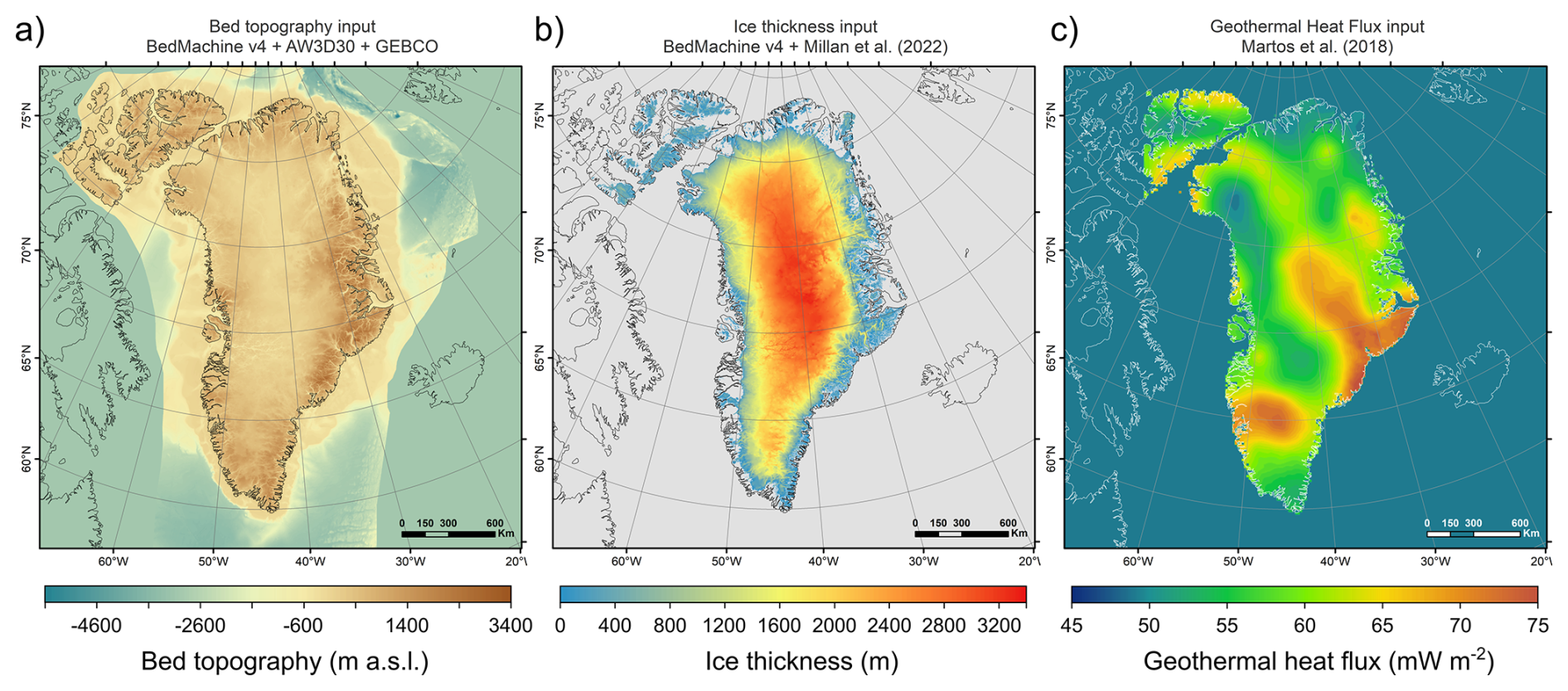
Figure 1 Time-independent and two-dimensional forcing fields used as inputs for present-day bed elevation (a), ice thickness (b; Morlighem et al., 2017; Millan et al., 2022), and geothermal heat flux (c; Martos et al., 2018). Bed elevation (a) is estimated by merging several products. Topography under the contemporary GrIS is from BedMachine v4 (Morlighem et al., 2017; spatial resolution: 150 m). For terrestrial regions with no GrIS cover, we use the ALOS World 3D 30 m Digital Elevation Model (DEM; Tadono et al., 2014). Present-day periphery ice is removed using thickness estimates from Millan et al. (2022). For other regions (ice-free ocean and other landmasses), we use the 15 arcsec resolution General Bathymetric Chart of the Oceans (GEBCO Bathymetric Compilation Group 2022, 2022). These datasets are resampled (to 5 × 5 km) using cubic convolution (Keys, 1981).

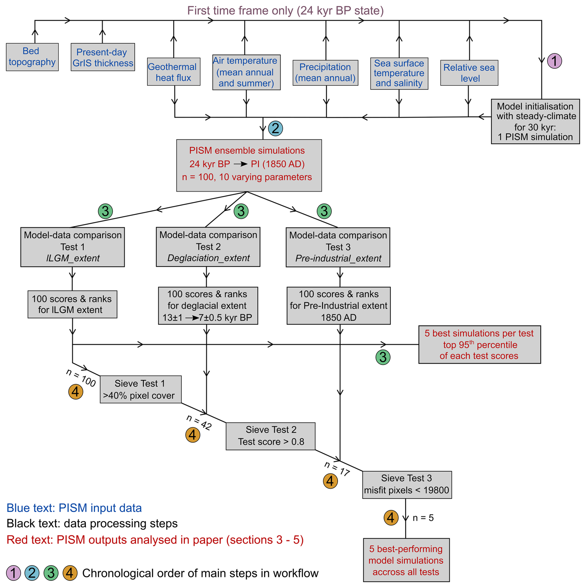
Figure 2 Flowchart diagram illustrating the methodological workflow followed in this study's modelling experiment including input datasets (step 1), model initialisation (step 1), transient ensemble simulations modelling (step 2) and post-processing steps including model-data comparison (step 3) and ensemble sieving (step 4). The reader is referred to the methods section for more details.

2.1.1 Ice flow

To model ice flow, PISM uses a hybrid stress balance scheme that combines the Shallow Ice Approximation (SIA) and the Shallow Shelf Approximation (SSA) (Bueler and Brown, 2009). PISM also features an enthalpy-based and three-dimensional formulation of thermodynamics enabling the modelling of polythermal ice and basal melt (Aschwanden et al., 2012). For ice rheology ($\dot{\mathit{ϵ}})$, we use the default Glen-Paterson-Budd-Lliboutry-Duval flow law,

$$\begin{array}{}\text{(1)}& {\dot{\mathit{ϵ}}}_{i,j}=E\cdot A\left(T,\mathit{\omega }\right){\mathit{\tau }}_{\mathrm{e}}^{n-\mathrm{1}}{\mathit{\tau }}_{i,j},\end{array}$$

where n is the flow-law exponent, E a flow enhancement factor, Athe Arrhenius factor (ice softness) determined by the liquid water content, ω, and ice temperature, T, while τ and τ_e represent the deviatoric and effective stresses, respectively (Aschwanden et al., 2012). In our ensemble, we vary E uniformly for both the SIA and SSA (see Sect. 2.3) and keep n=3 as default.

2.1.2 Boundary conditions

The ice-bed interface

We use the slip law of Zoet and Iverson (2020), which considers both mechanisms of glacier sliding over rigid beds and subglacial till deformation with minimal parameterisation and no required knowledge of the bed type. In PISM, this law is formulated as

$$\begin{array}{}\text{(2)}& {\mathit{\tau }}_{\mathrm{b}}=-{\mathit{\tau }}_{\mathrm{c}}{\displaystyle \frac{\mathit{u}}{{\left(\left|\mathit{u}\right|+u_{\mathrm{t}}\right)}^q|\mathit{u}{|}^{\mathrm{1}-q}}},\end{array}$$

where τ_b is the basal shear stress, τ_c the basal yield stress, u the slip velocity and u_t the threshold velocity at which shear stress equals the Coulomb shear strength of the till. In our simulations, u_t is kept constant at 50 m yr⁻¹ (Khroulev and The PISM authors, 2020; Zoet and Iverson, 2020) while q varies between simulations (see section 2.3). We account for space- and time-dependent basal yield stress, τ_c, controlled primarily by a simple hydrology model (Tulaczyk et al., 2000) which determines the effective pressure, N_till, from the till-pore water content obtained by storing basal melt locally up to a threshold (here set to 2 m). With this simplified parameterisation, water is not conserved as water reaching above the threshold is lost permanently. The basal water thickness in the till layer, W_till, is computed from the basal melt rate, m_b, obtained from the enthalpy, as follows:

$$\begin{array}{}\text{(3)}& {\displaystyle \frac{\partial W_{\mathrm{till}}}{\partial t}}={\displaystyle \frac{m_{\mathrm{b}}}{{\mathit{\rho }}_{\mathrm{w}}}}-C_{\mathrm{dr}},\end{array}$$

where C_dr is a simple decay rate parameter and ρ_w is the density of fresh water. Secondly, τ_c is also controlled by the till friction angle, ϕ, i.e. the frictional strength of basal till materials (Cuffey and Paterson, 2010)

$$\begin{array}{}\text{(4)}& {\mathit{\tau }}_{\mathrm{c}}=\tan \left(\mathit{\varphi }\right)N_{\mathrm{till}}.\end{array}$$

By assuming basal materials in valley troughs are generally weaker than towards mountain tops, we parameterise ϕ as a piece-wise linear function of bed elevation, b, (after Aschwanden et al., 2013, 2016; Huybrechts and de Wolde, 1999)

$$\begin{array}{}\text{(5)}& \begin{array}{rl}& \mathit{\varphi }\left(x,y\right)=\\ & \left\{\begin{array}{l}{\mathit{\varphi }}_{\min },\\ {\mathit{\varphi }}_{\min }+\left(b\left(x,y\right)-b_{\min }\right)M,\\ {\mathit{\varphi }}_{\max },\end{array}\right.\begin{array}{l}b\left(x,y\right)\le b_{\min },\\ b_{\min }<b\left(x,y\right)<b_{\max },\\ b_{\max }\le b\left(x,y\right),\end{array}\end{array}\end{array}$$

where $M=({\mathit{\varphi }}_{\max }-{\mathit{\varphi }}_{\min })/(b_{\max }-b_{\min })$. We set elevation thresholds (b_min,b_max) to −400 and 500 m a.s.l., respectively, while ϕ thresholds (ϕ_min,ϕ_max) are simulation-dependent (Table 1, see Sect. 2.3). This PISM parameterisation was shown to produce flow velocities consistent with observations for major GrIS glaciers (Aschwanden et al., 2016).

Bed elevation is obtained by merging topographies from BedMachine v4 (Morlighem et al., 2017), the ALOS World 3D 30 m Digital Elevation Model (DEM; Tadono et al., 2014), and the General Bathymetric Chart of the Oceans (GEBCO Bathymetric Compilation Group 2022, 2022). The reader is referred to Fig. 1 for more details. To avoid modelling large non-Greenlandic ice bodies, Iceland and Baffin Island are removed (Fig. 1). We however include the Innuitian Ice Sheet (IIS) as it coalesced with the GrIS (Jennings et al., 2011) and the two ice sheets dynamically impacted each other (Bradley et al., 2018). Modern icecaps on Ellesmere Island are removed using ice thickness estimates from Millan et al. (2022). Finally, we use a two-dimensional and time-independent geothermal heat flux data from Martos et al. (2018) (Fig. 1). This dataset ranges from 0.049 to 0.073 W m⁻², and is consistent with a plume track (the Iceland hotspot) that crossed Greenland from NW to SE. As this reconstruction does not feature geothermal heat flux data outside modern land areas, a constant value of 50 mW m⁻², the lowest values in the original dataset, is uniformly prescribed in ocean-covered regions (Fig. 1). We run PISM at the horizontal resolution of 5 × 5 km (grid size: 620 × 620), with 101 vertical ice layers using quadratic concentration at the base.

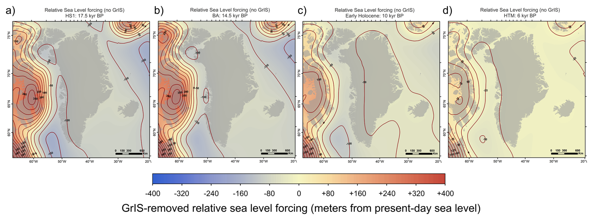
Figure 3 GrIS-removed (non-local components) relative sea-level forcing data for four different time slices and given as input to our transient ensemble simulations. These snapshots show the relative sea-level prior to adding the GrIS-specific contribution to GIA-induced relative sea-level change during our transient ensemble simulations (see methods section). Positive offset values (red) indicate isostatic bed depression relative to present and thus higher relative sea-levels than today, while negative offset values (blue) indicate isostatic bed uplift relative to present (e.g. on a peripheral bulge) and thus lower relative sea-levels than today. Snapshots are shown for the the HS 1 cooling event (a), the BA warming event (b; 14.5 kyr BP), the early Holocene (c; 10 kyr BP), and the HTM warming event (d; 6 kyr BP). All model input data fields are re-projected to EPSG:3413 and resampled to a 5 × 5 km resolution using cubic convolution.

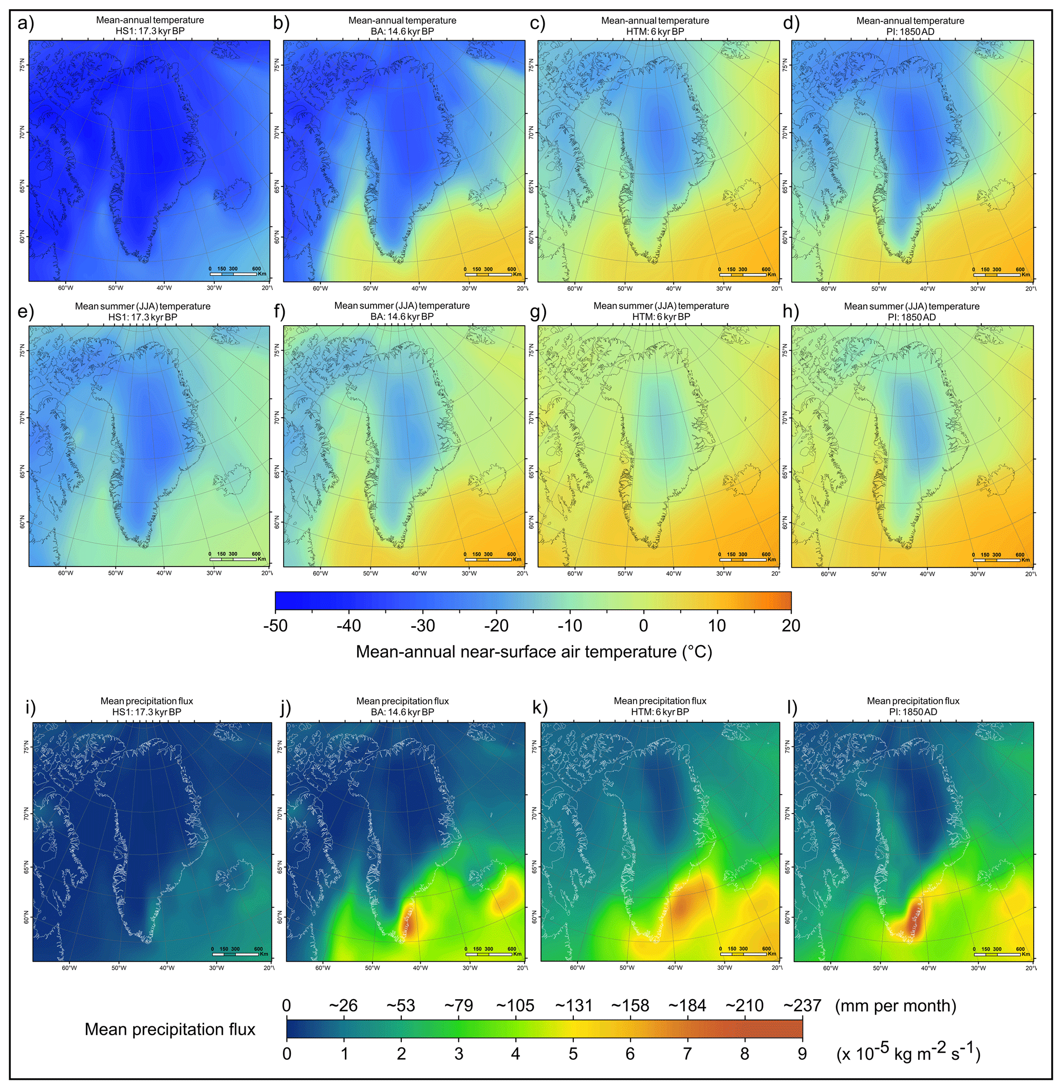
Figure 4 Two-dimensional fields of mean-annual surface air temperature (a–d), mean-summer surface air temperature (JJA mean; e–h), and mean annual precipitation flux (i–l) data used as input in our modelling experiment, derived from iCESM transient and equilibrium time slice simulations (see methods section), and shown as snapshots for the HS 1 cooling event (a, e, i), the BA warming event (b, f, j), the HTM warming event (c, g, k), and the PI (1850 AD; d, h, l). All climate input data fields are re-projected to EPSG:3413 and resampled to a 5 × 5 km resolution using cubic convolution.

The ice-atmosphere interface

To compute Surface Mass Balance (SMB) from time-dependent surface air temperature and precipitation (see Sect. 2.1.3), we use PISM's Positive-Degree-Day (PDD) model (Calov and Greve, 2005; Ritz, 1997). Precipitation when temperature is above 2 °C and under 0 °C is interpreted as rain and snow, respectively, with a linear transition between. Temperature and precipitation fields used to force the SMB are further described in Sect. 2.1.3. The fraction of surface melt that refreezes is set to 60 % (EISMINT-Greenland value; Ritz, 1997). Spatio-temporal variations in the standard deviation, σ, of daily temperature variability influences SMB (Arnold and MacKay, 1964). We parameterise σ to be a linear function of surface air temperature T (and indirectly, of ice surface elevation)

$$\begin{array}{}\text{(6)}& \mathit{\sigma }=aT+b.\end{array}$$

We assign b a value of 1.66 (after Seguinot and Rogozhina, 2014) and vary a as part of our ensemble (see Sect. 2.3).

The ice-ocean interface

For floating sectors of the modelled GrIS, sub-shelf melt is obtained by computing basal melt rate and temperature from thermodynamics in a boundary layer at the ice shelf base (Hellmer et al., 1998; Holland and Jenkins, 1999). This model, which does not consider sub-shelf circulation, uses three equations describing: (1) the energy flux balance, (2) the salt flux balance, and (3) the pressure- and salinity-dependent freezing point in the boundary layer. This sub-shelf melt parameterisation thus requires time-dependent fields of potential temperature and practical salinity (see Sect. 2.1.3.). More details can be found in Hellmer et al. (1998) and Holland and Jenkins (1999). Calving was a predominant ablation mechanism during the lLGM (∼ 21–15 kyr BP) and throughout the Late-Glacial, when the GrIS was mostly marine-terminating (Funder et al., 2011). Although the physical processes behind calving remain poorly understood, we here model it following similar PISM parameterisations as Albrecht et al. (2020) and Pittard et al. (2022). Firstly, floating ice at the calving front thinner than a given threshold is calved (see Sect. 2.3). Secondly, we use the strain-rate-based eigen calving law (Albrecht and Levermann, 2014; Levermann et al., 2012) to determine the average calving rate, c, based on the horizontal strain rate, ${\dot{\mathit{ϵ}}}_{\pm }$, derived from SSA-velocities, and a constant, K, integrating ice material properties at the calving front

$$\begin{array}{}\text{(7)}& c=K{\dot{\mathit{ϵ}}}_{+}{\dot{\mathit{ϵ}}}_{-},{\dot{\mathit{ϵ}}}_{\pm }>\mathrm{0}.\end{array}$$

We assign K a value of 5 × 10¹⁷ m s⁻¹ (after Albrecht et al., 2020; Pittard et al., 2022). While a von Mises stress – type calving law may be more appropriate for fjord-terminating glaciers (e.g. Aschwanden et al., 2019), the GrIS expanded over continental shelves and was entirely marine-terminating during the lLGM, thus forming wide ice shelves comparable to Antarctica today (Jennings et al., 2017). As the ice sheet was in this configuration for more than half our simulated timeframe, we rely on the eigen calving law throughout our simulations. Following Albrecht et al. (2020), we further restrict ice-shelf extent by calving ice when bathymetry exceeds 2 km, with the exception of Baffin Bay.

The grounding line location is determined by computing a flotation criterion (Khroulev and The PISM authors, 2020). This criterion depends on water depth, defined as the vertical distance between the geoid and the solid earth surface (Mitrovica and Milne, 2003). Around Greenland, and for our timeframe (24–0 kyr BP), spatio-temporal variations in water depth result from changes in the global mean sea level and GIA-induced deformation of the solid earth (Rovere et al., 2016). The latter can result from variations in GrIS mass (local sources), and the influence of the neighbouring Laurentide Ice Sheet (LIS) and IIS, responsible for spatially and temporally variable sea level around Greenland (non-local sources)(Bradley et al., 2018). During and following glaciations, non-local contributions can be significant, as Greenland is located on the eastern peripheral forebulge generated by the LIS (Simpson et al., 2009; Lecavalier et al., 2014) (Fig. 3). We thus combine at each time step the non-local relative sea level signal calculated from an offline GIA model with the local GrIS-driven signal, enabling to compute the final water depth and resulting flotation criterion (Fig. 3).

For the local GrIS signal, we use PISM's Lingle-Clark-type viscoelastic deformation model (Lingle and Clark, 1985; Bueler et al., 2007). We use default lithosphere flexural rigidity and mantle density values of 5 × 10²⁴ N m⁻¹ and 3300 kg m⁻³, respectively. For mantle (half-space) viscosity, we use a value of 5 × 10²⁰ Pa s⁻¹, consistent with Lambeck et al. (2017). To calculate non-local sea level changes across our domain, we run an offline GIA model. This model was run at a resolution of 512° and solves the generalized sea level equation (Mitrovica and Milne, 2003; Kendall et al., 2005) accounting for sea level change in regions of retreating marine-based ice, perturbations to the Earth's rotation vector, and time-varying shoreline migration. For the input ice sheet reconstruction, we use a hybrid reconstruction (Lambeck et al., 2014, 2017), where the GrIS is removed from the North American ice sheet reconstruction. We use a 1D viscoelastic earth model with a lithosphere thickness of 96 km and upper and lower mantle viscosities of 5 × 10²⁰ and 1 × 10²² Pa s⁻¹, respectively. This offline model is used to produce two-dimensional input sea level offsets from the present-day sea level between 24 kyr BP and the PI, at 500 yr temporal resolution. PISM uses these offsets to compute the final relative sea level after computing local GIA deformation.

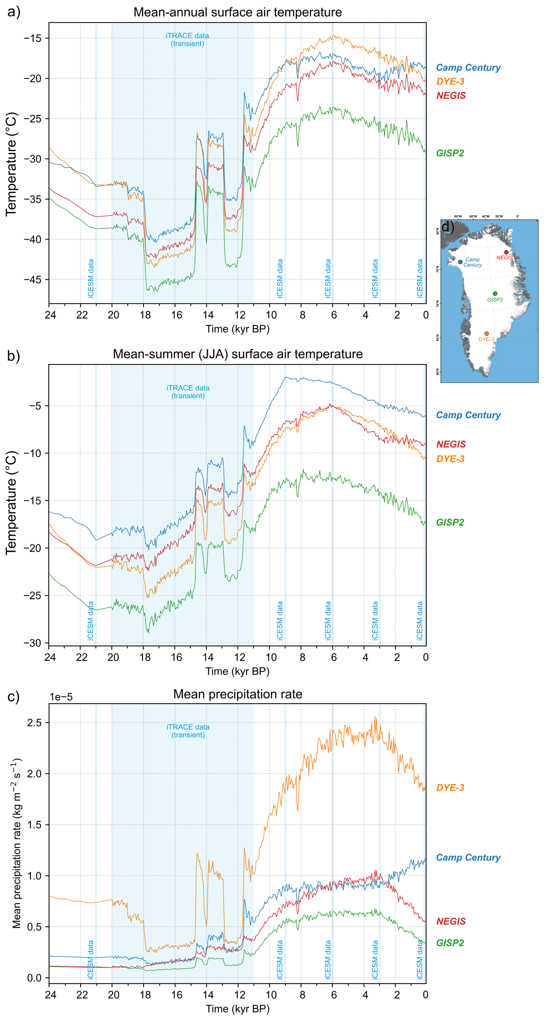
Figure 5 Time series of mean-annual (a) and mean-summer (JJA-mean; b) surface air temperature data used as forcing in our ensemble simulations, at 4 different locations of the ice sheet (shown on inset: d). Transparent blue bands highlight time windows covered by iCESM climate data. In between these data points, forcing fields are approximated using a spatially-variable glacial index scheme (see methods section).

2.1.3 Atmospheric and oceanic forcings

Air temperature and precipitation

The SMB PDD model used here is forced with time-dependent fields of surface air temperature and total precipitation (Figs. 4–7). We use pre-existing simulations from iCESM (Brady et al., 2019) run globally at a horizontal resolution of 1.9 × 2.5° (latitude × longitude) for the atmosphere and a nominal 1° for oceans. We use full forcing simulations, i.e. including ice sheet (from ICE-6G: Peltier et al., 2015), orbital (Berger, 1978), greenhouse gases (Lüthi et al., 2008) and meltwater forcings. Between 20 and 11 kyr BP, we use monthly-resolution output from the iTRACE experiment, ran with iCESM 1.3 (He et al., 2021a, b). Thanks to an improved climate model, higher resolution, and the addition of water isotopes, iTRACE simulates a climate over Greenland that is more data-consistent (He et al., 2021a) than the former CESM simulation of the last deglaciation TRACE-21 (Liu et al., 2009). Additionally, we use output from five equilibrium time-slice simulations ran at 21 kyr BP (iCESM 1.3), at 9, 6, and 3 kyr BP (iCESM 1.2), and at the PI (1850 AD, iCESM 1.3) (Fig. 4).

To create continuous forcing over remaining data gaps in time, we apply a glacial-index-type approach (Niu et al., 2019; Clark et al., 2022) and linearly scale our climate fields proportionally to variations in independent climate reconstructions in a space-dependent manner i.e. building an interpolation for each individual grid cell (Fig. 5). Between 24 and 21 kyr BP, we use surface air temperature and δ¹⁸O reconstructions of Osman et al. (2021) to scale variations in temperature and precipitation fields, respectively. For data gaps between 21 kyr BP and the PI (e.g. 11–9 kyr BP), we use the seasonally-resolved Greenland-wide temperature and precipitation reconstruction of Buizert et al. (2018) as glacial index. The interpolation is computed as such: for each temporal gap in iCESM-derived data (e.g. 11–9 kyr BP), and for each grid cell, we construct a continuous forcing A(t) between two iCESM-derived values C₁ and C₂ at times t₁ and t₂. This is achieved by scaling the linear interpolation between C₁ and C₂ with the relative excursions of an independent reconstruction B(t) (e.g. data from Buizert et al., 2018) from its own linear trend:

$$\begin{array}{}\text{(8)}& \begin{array}{rl}A\left(t\right)& =\left[C_{\mathrm{1}}+\left(C_{\mathrm{2}}-C_{\mathrm{1}}\right){\displaystyle \frac{t-t_{\mathrm{1}}}{t_{\mathrm{2}}-t_{\mathrm{1}}}}\right]\\ & \cdot {\displaystyle \frac{B\left(t\right)}{B\left(t_{\mathrm{1}}\right)+\left(B\left(t_{\mathrm{2}}\right)-B\left(t_{\mathrm{1}}\right)\right)\frac{t-t_{\mathrm{1}}}{t_{\mathrm{2}-t_{\mathrm{1}}}}}}.\end{array}\end{array}$$

Note this method requires temperature units of Kelvin to avoid negative °C values causing interpolation distortions. As a result, we produce time-dependent, two-dimensional fields of mean annual and mean summer (JJA) surface air temperature and precipitation rate, continuous between 24 kyr BP and PI (Figs. 4–7). From mean annual and summer temperatures, our SMB model reads a cosine yearly cycle to generate a seasonality signal.

Ocean temperature and salinity

To compute sub-shelf melt, our PISM parameterisation (Holland and Jenkins, 1999) requires time-varying fields of potential ocean temperature and salinity (see Sect. 2.1.2). For the ocean temperature, we use the LGM-to-present ensemble-mean sea surface temperature (SST) reconstruction of Osman et al. (2021), yielding a 200-year temporal resolution and nominal 1° spatial resolution (Fig. 6). This re-analysis uses Bayesian proxy forward models to perform an offline data assimilation (using 573 globally-distributed SST records) on climate model priors; i.e. a set of iCESM 1.2 and 1.3 simulations (Zhu et al., 2017; Tierney et al., 2020). Whilst we acknowledge sub-shelf ocean temperature would be a more appropriate forcing than SST, their does not yet exist a Greenland-wide time- and space-dependent sub-shelf ocean temperature reconstruction which assimilates proxy data between 24 kyr BP and the PI. The transient and data-assimilated nature of the SST reconstruction by Osman et al. (2021) was thus preferred to iCESM outputs of shelf-depth ocean temperature (e.g. Tabone et al., 2024). For ocean surface salinity, we use iCESM outputs, following the same methodology as described above. Due to a lack of independent proxy data for ocean salinity, we however use linear interpolation rather than a glacial index scheme to bridge the temporal data-gaps in salinity data (Fig. S1), which are located outside of the transient iTRACE data (20–11 kyr BP) and equilibrium iCESM simulations (21, 9, 6, 3 kyr BP and PI).

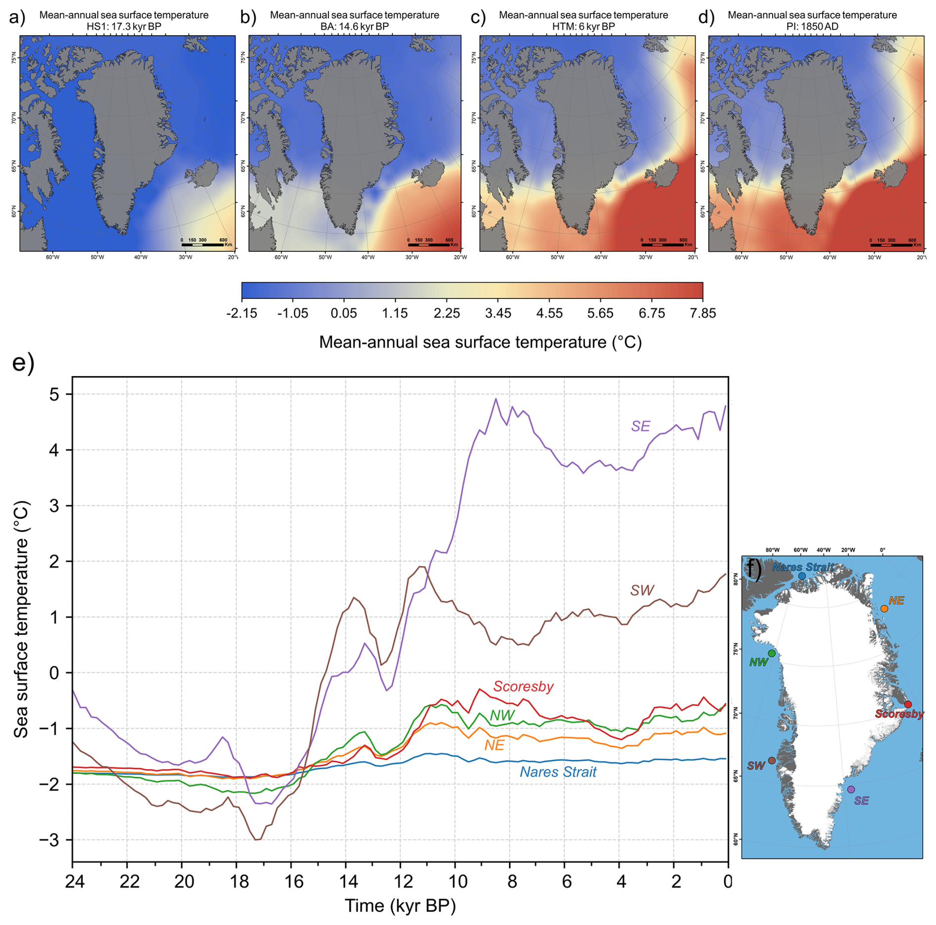
Figure 6 Mean annual sea-surface temperature input data used as forcings in our transient ensemble simulations (Osman et al., 2021). These data are shown as snapshots for the HS 1 cooling event (a), the BA warming event (b), the HTM warming event (c), and the PI (1850 AD; d). All climate and ocean input data fields are re-projected to EPSG:3413 and resampled to a 5 × 5 km resolution using cubic convolution. (e) displays time series of mean annual sea-surface temperature extracted from our two-dimensional input forcing fields, for six distinct locations taken from different ocean basins offshore the present-day GrIS (as shown by the inset: f). Time series of sea-surface salinity data, used in our sub-shelf melt computations and obtained form iCESM outputs, are also shown for the same six locations in Fig. S1.

2.2 Model initialisation

For model initialisation, we simulate a GrIS in balance with boundary conditions at 24 kyr BP, the starting year of our transient simulations, chosen to be significantly earlier (∼ 9 kyr) than the lLGM (17.5–15 kyr BP; Lecavalier et al., 2014). We start from present-day GrIS thickness and bedrock topography (Fig. 1b) and run a 30 kyr-long simulation using the parameterisations described above, fixing ensemble-varying parameters to their mid-range values (Table 1). After 30 kyr with a static climate (from 24 kyr BP), modelled surface and basal ice velocities are stable across the domain, while mass flux rates in glacierised areas are near zero. Basal mass flux for grounded and sub-shelf ice as well as surface melt, accumulation and runoff rates all reach steady state. The spun-up grounded GrIS area reaches 2.27 × 10⁶ km², while grounded-ice volume approximates 8.22 m sea-level-equivalent (SLE), ∼ 0.8 m above its present-day volume (7.42 ± 0.05 m SLE; Morlighem et al., 2017). In this study, grounded GrIS volume calculations, expressed as sea-level contribution (m SLE), exclude ice under flotation (using the PISM-derived time-dependent flotation criterion), the IIS, peripheral glaciers and icecaps, and any ice thinner than 10 m (after Albrecht et al., 2020). We use ice density, seawater density, and ocean surface area values of 910 kg m⁻³, 1027 kg m⁻³, and 3.618 × 10⁸ km² (Menard and Smith, 1966), respectively. This spun-up GrIS is used as initial condition for all ensemble transient simulations. The 30 kyr equilibrium spinup limited us computationally to this single initial state at 24 kyr BP with ensemble-varying parameters fixed to mid-range values. Although adjusting parameters in subsequent transient runs can generate instabilities in the first simulation years, equilibrium with parameterisations is reached within the first centuries, as evidenced by model outputs (e.g. GrIS volume) from different ensemble runs diverging notably prior to 23 kyr BP, and should thus not markedly affect the modelled lLGM or deglacial dynamics.

2.3 Ensemble design

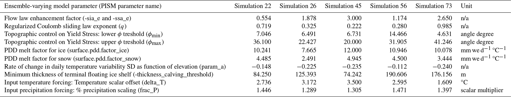
Numerical ice-sheet modelling is governed by a plethora of parameters, many of which are poorly constrained by physical processes or empirical data. Uncertainties from subjective parameter configurations are large, and generally greater in paleo simulations, due to a lack of observational data (Tarasov et al., 2012). To minimise biases in parameter choices and to assess model-data fit (see Sect. 2.4) using a wide range of parameter configurations, we generate an ensemble of 100 simulations with 10 varying parameters (Table 1). We use Latin hypercube sampling (Iman, 2008; Stein, 1987) with the maximin criterion (van Dam et al., 2007) to ensure homogeneous sampling of the high-dimensionality parameter space, while minimising potential redundancies. The 10 ensemble-varying parameters were drawn from five groups:

• Ice dynamics: We alter the flow law (Eq. 1) enhancement factor (E) uniformly for both the SIA and SSA using a range (0.5–3) bracketing the value E=1.25 found to produce best fit with contemporary GrIS flow speeds (Aschwanden et al., 2016). We vary the sliding law exponent q (Eq. 3) between 0.01 and 1, which permits continuously altering the dependency of basal shear stress on sliding velocity from nearly purely-plastic to linear.

• Basal yield stress: To alter the impact of bed elevation (and bed strength) on basal yield stress between simulations, we vary ϕ_min and ϕ_max (Eq. 4) between 4–15° and 20–45°, respectively, which bracket values obtained by Aschwanden et al. (2016) for present-day GrIS hindcasting.

• SMB: Based on present-day GrIS surface melt, PDD snow and ice melt factors vary between 2–5 and 5–12 mm we d⁻¹ °C⁻¹, respectively (Braithwaite, 1995; Fausto et al., 2009; Aschwanden et al., 2019). We also vary coefficient a in Eq. (5) between −0.25 and −0.1, thus modifying the impact of temperature change on the standard deviation of daily temperature variability (σ), following the relationship established by Seguinot and Rogozhina (2014).

• Calving: Preliminary testing revealed that varying the minimum thickness threshold of ice shelf fronts had a greater impact on modelled GrIS extent than modifying the eigen calving law constant, K (Eq. 6). The thickness threshold was thus retained as an ensemble parameter and is varied between 25 and 200 m, based on observations (Motyka et al., 2011; Morlighem et al., 2014).

• Climate forcing: Paleo-climate simulations from earth-system models can have biases, for instance due to possibly inaccurate geometry of the paleo-ice-sheet boundary conditions (Buizert et al., 2014; Erb et al., 2022; He et al., 2021a). To account for this, we apply perturbations to climate fields using space-independent temperature and precipitation offsets as ensemble-varying parameters (Table 1). Based on surface air temperature variability over Greenland (1 SD) in Osman et al. (2021)'s ensemble, we vary temperature fields by −3.5 to +3.5 °C (Table 1). Preliminary simulations showed a high sensitivity of modelled GrIS extent and volume to precipitation changes. We thus vary precipitation using a wide range of offsets, i.e. between 20 % and 200 % input precipitation.

Table 1 List of ensemble-varying parameters (n=10) and ranges sampled with the Latin Hypercube technique. Note the references cited here did not necessarily employ the same parameter values. They were used as primary source of knowledge for making a final decision on the chosen parameter ranges to sample from in this study. For more justification and details, the reader is referred to the methods section. n/a: not applicable.

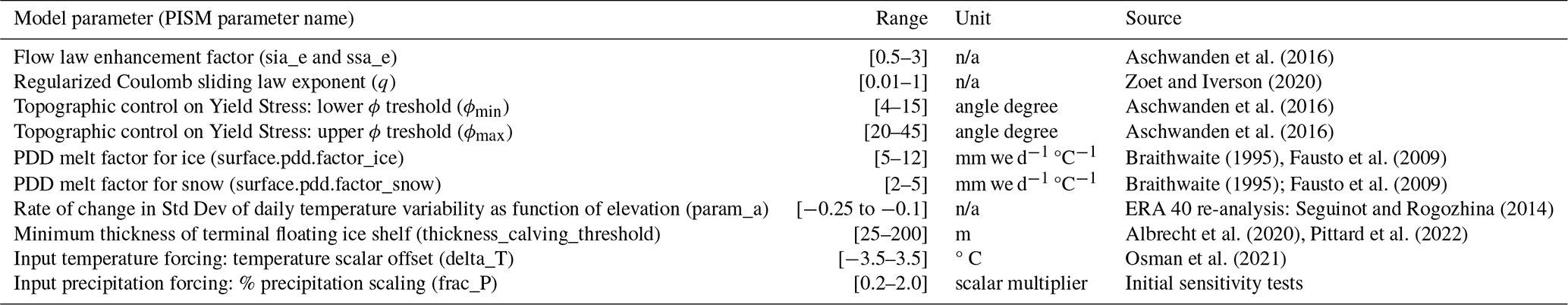
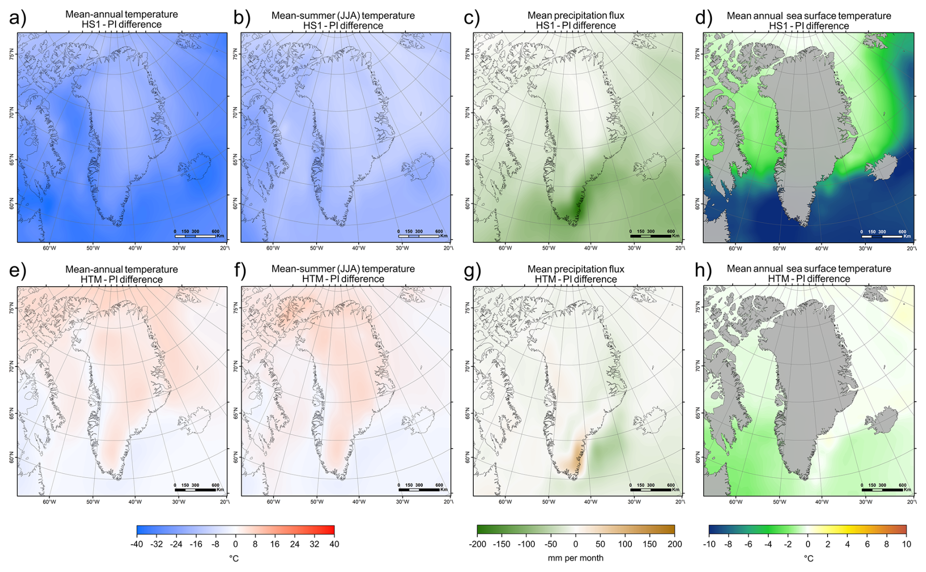
Figure 7 Fields of differences in input mean annual (a, e) and mean summer (JJA-mean; b, f) surface air temperature, precipitation rate (c, g), and sea-surface temperature (d, h) between Heinrich Stadial 1 (17.5 kyr BP: peak cooling during our simulations) and the PI era (1850 AD) for (a)–(d), and between the Holocene Thermal Maximum (6 kyr BP: peak warming during our simulations) and the PI for (e)–(h).

2.4 Model-data comparison scheme

Isolating best-fit ensemble simulations requires a quantitative assessment of model-data agreement on past GrIS behaviour. Here, each simulation is scored using three chronologically distinct tests, described below. Before testing, we remove the IIS and ice thinner than 10 m from modelled thickness fields. Because former GrIS ice-shelf extent is poorly constrained, and empirical datasets used here only constrain grounded GrIS extent, we also exclude floating ice (post-simulation) and restrict all ice-extent analyses to grounded ice for the remainder of the study. Modelled ice-shelf extent at selected time periods is nonetheless shown in Figs. 22 and 23.

• The local-LGM extent test: This test evaluates the fit between simulations and grounded GrIS extent during the lLGM (∼ 21–15 kyr BP, depending on region; e.g. Funder et al., 2011; Ó Cofaigh et al., 2013; Hogan et al., 2016; Jennings et al., 2017; Sbarra et al., 2022). Because the GrIS was fully marine-terminating, data constraining its past extent are rare and challenging to obtain (Sbarra et al., 2022). Given this uncertainty, we define a conservative lLGM mask spanning the area between the outermost PaleoGrIS 1.0 isochrone (∼ 14–13 kyr BP) (Leger et al., 2024), which reconstructs margins following initial deglaciation, and the continental shelf break, a likely maximum limit (Fig. 8). Given dating challenges (Jennings et al., 2017), no chronology is considered in this test, rather only absolute extent. For each simulation, we compute the percentage of mask pixels covered by grounded ice at any time, then normalise these values to produce a 0–1 score (Fig. 9). High-scoring simulations reconstruct a more extensive grounded GrIS, covering larger parts of the mid- to outer continental shelves, thus yielding a more accurate lLGM geometry (Fig. 9).

• The deglaciation extent test: This test evaluates simulations against an empirical reconstruction of GrIS retreat during the last deglaciation (∼ 15–5 kyr BP). We use ATAT v1.1 (Ely et al., 2019) to score simulations against the PaleoGrIS 1.0 isochrone reconstruction (Leger et al., 2024), spanning 13 ± 1 to 7 ± 0.5 kyr BP. We use the “isochrone buffer” product, a mask-based version of the reconstruction suited for models with > 1 km resolution (see Fig. 15 in Leger et al., 2024). Three ATAT output statistics are equally weighted into a final normalised 0–1 score: (i) the percentage of PaleoGrIS 1.0 buffer pixels covered by grounded ice (periphery glaciers removed), (ii) the percentage of these pixels matching within chronological error, and (iii) the Root-Mean Squared Error in retreat timing (see Ely et al., 2019: Table 4). This test thus evaluates whether modelled GrIS margins retreat across the correct regions and at the correct time and rate (Figs. 8, 9).

• The Pre-Industrial extent test: This test evaluates simulations against the PI (1850 AD) GrIS extent. We compute the difference in grounded ice extent between the present-day GrIS (BedMachine v4 re-sampled to 5 km) and each simulation's final frame (1850 AD). Although these states differ by ∼ 150 years, we assume the offset is negligible relative to the 24 kyr simulation length and the 5 km spatial uncertainty of both products, which likely exceeds the true extent difference. We then count pixels where simulated PI grounded ice is either more or less extensive than the present-day margin (Figs. 8, 9). The total misfit pixel count is normalised into a final 0–1 score.

To isolate overall best-fit simulations, we apply a chronologically-ordered sieving approach and sequentially remove simulations that do not meet thresholds at each test. Simulations first pass the local-LGM extent test if mask pixel coverage exceeds > 40 %. Of these, only runs scoring > 0.8 (out of 1) at the deglaciation extent test are retained. Of these, only simulations with an extent misfit area < 495 × 10³ km² (i.e. < 19800 misfit pixels) at the Pre-Industrial extent test, are retained. Thresholds were set such that 60 %–70 % of simulations are removed by each sieve while retaining five best-fit runs (upper 95th percentile of comparison scores). This strategy avoids selecting simulations that fit the present-day state well but achieve it through unrealistic paleo-evolution.

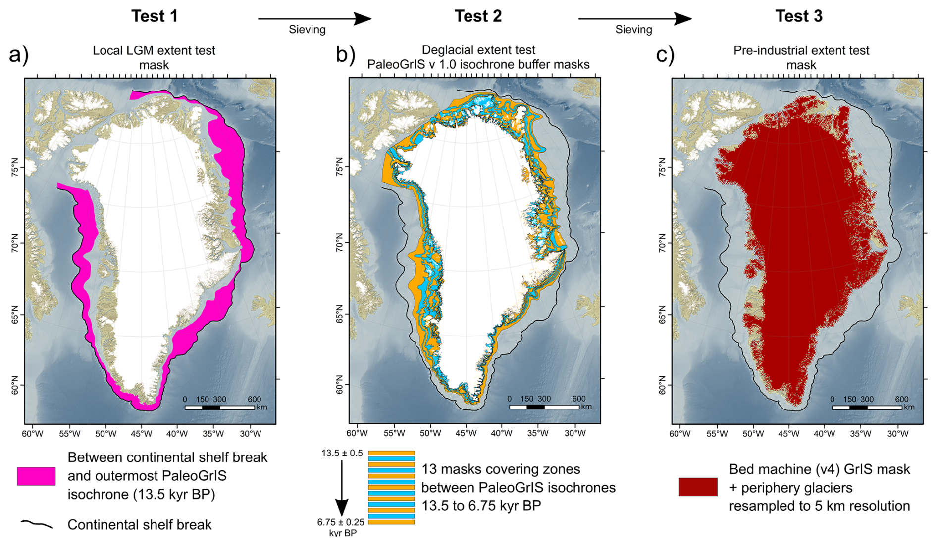
Figure 8 Maps highlighting the spatial coverage of masks derived from empirical datasets (Morlighem et al., 2017; Leger et al., 2024) and used for our three distinct quantitative model-data comparisons tests: i.e. the local-LGM extent test (a), the deglacial extent test (b), and the pre-industrial extent test (c). Bathymetry data shown in these maps is from the 15 arcsec resolution General Bathymetric Chart of the Oceans (GEBCO Bathymetric Compilation Group 2022, 2022). The white masks highlight all present-day ice cover.

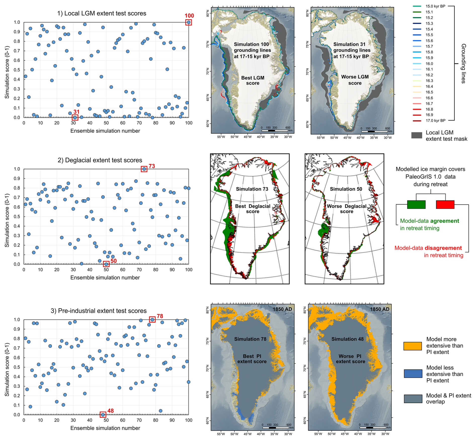
Figure 9 Ensemble simulation scores at our three model-data comparison tests (local-LGM extent test, deglacial extent, and PI extent test) and example results illustrated for both the best-scoring and worst-scoring ensemble simulations, at each test. Note that for the PI-extent test, the 2D mask used as empirical data and described in this figure as the “PI extent” is the grounded ice extent of the present-day GrIS mask from BedMachine v4 (Morlighem et al., 2017) re-sampled to 5 km resolution, with periphery glaciers removed. While the true PI and present-day extents represent GrIS states that differ by ∼ 150 years, we here consider this difference to be negligible given our 24 kyr-long simulations and the 5 × 5 km spatial uncertainty inherent to both products. That uncertainty, once propagated, likely exceeds the extent offset between the two states. Bathymetry and topography data shown in these maps are from the 15 arcsec resolution General Bathymetric Chart of the Oceans (GEBCO Bathymetric Compilation Group 2022, 2022).

3 Insights into past Greenland-Ice-Sheet history

3.1 Modelled Greenland Ice Sheet during the local LGM

3.1.1 Ensemble-wide trends

All ensemble simulations (n=100) model an increase (of up to ∼ 23 %) in grounded GrIS extent between the global LGM (i.e. 24–21 kyr BP) and the lLGM, here modelled between 17.5 and 16 kyr BP (Fig. 10). This is consistent with the timing of maximum GrIS volume and extent in other recent modelling studies (e.g. 16.5 kyr BP in Lecavalier et al., 2014; 17–17.5 kyr BP in Yang et al., 2022). Here, modelled GrIS maximum expansion is synchronous with the Heinrich Stadial 1 (HS1: ∼ 18–14.7 kyr BP: He et al., 2021a) cooling event. In our prescribed climate forcing (iCESM-derived), HS1 is associated with decreases in mean annual air temperatures of between 5 and 7 °C over the GrIS (Figs. 4, 5), and reductions in sea surface temperatures of up to 1 °C in ocean basins surrounding Greenland (Fig. 6). In nearly all ensemble simulations, HS1 cooling forces modelled surface accumulation rates to increase between 24 and 16 kyr BP (by up to 200 % for certain simulations) and causes reduced sub-shelf melt (by up to 350 %), between 18 and 16 kyr BP (Fig. 11).

3.1.2 Insights from local LGM best-fit simulations

In this section, we refer to “lLGM best-fit simulations” as the five best-scoring simulations at the local-LGM extent test (Figs. 12, 13, 14–16).

Grounded GrIS extent during lLGM

Our lLGM best-fit simulations yield maximum grounded GrIS areas that range between 2.80 and 2.85 million km² (excluding the IIS) (Fig. 12), ∼ 1.65 times the present-day area (1.71 million km²; Morlighem et al., 2017). Agreement with empirical data on lLGM extent is relatively good: our simulations are 4 ± 0.7 % and 10 ± 0.6 % less extensive than the minimum and maximum lLGM GrIS extents reconstructed in PaleoGrIS 1.0 (Leger et al., 2024) (Figs. 13, 16), respectively. Remaining misfits occur mainly in NE Greenland, where no simulation produces grounded ice extending to the mid-to-outer continental shelf during the lLGM (Figs. 13, 16, 17), contrary to recent empirical evidence (e.g. Hansen et al., 2022; Davies et al., 2022; Roberts et al., 2024; Ó Cofaigh et al., 2025). These studies indicate grounded margins reached ∼ 100–200 km farther east than in our most extensive simulations. This suggests the true lLGM (∼ 17–16.5 kyr BP) grounded GrIS area was likely 2.9–3.1 million km², consistent with the Huy3 model (Lecavalier et al., 2014).

Along the Western GrIS margin, from offshore Uummannarsuaq in the South (Cape Farewell) to offshore Kangaarasuk in the North (Cape Atholl), all lLGM best-fit simulations (and much of the ensemble) model a grounded margin reaching the continental shelf edge during the lLGM (Figs. 13, 14, 16). This agrees with empirical constraints on the western GrIS LGM extent (e.g. Ó Cofaigh et al., 2013; Rinterknecht et al., 2014; Sbarra et al., 2022), whereby both data and modelling increasingly suggest the grounded GrIS reached the shelf edge along its entire western margin. Our lLGM best-fit simulations also produce extensive ice shelves extending across Baffin Bay during that time. As the LGM LIS also contributed major ice flux into Baffin Bay from the west (Dalton et al., 2023), it seems plausible the bay was fully covered by ice shelves between 18 and 16 kyr BP. Toward the relatively shallow Davis strait saddle (500–600 m below present-day sea level), offshore CW Greenland, four of five lLGM best-fit simulations model grounded ice extending beyond the shelf break and onto the saddle (Fig. 13). If the LIS similarly extended east from Baffin Island, grounded ice from both ice sheets may have coalesced over Davis Strait, as modelled in some previous studies (e.g. Patterson et al., 2024; Gandy et al., 2023).

We find that along the western GrIS margin (e.g. Jakobshavn, Uummannaq), modelled ice streams (≥ 800 m yr⁻¹) show little variation in flow velocity, shape, or trajectory across lLGM best-fit simulations. In contrast, SE and CE Greenland display greater inter-simulation variability: the modelled Helheim, Kangerlussuaq, and Scoresby ice streams differ more in velocity, flow paths, and fast-flow corridor dimensions, indicating stronger sensitivity to ensemble parameters and greater uncertainty in lLGM ice dynamics (Fig. 16). In all five lLGM best-fit simulations, grounded ice from these three eastern ice streams reaches the continental shelf edge during maximum expansion (Figs. 13, 16). However, none simulate margins extending onto the shelf between the Kangerlussuaq and Scoresby ice streams, offshore the Geikie Plateau peninsula (Figs. 13, 16), a region with sparse geochronological constraints (Leger et al., 2024), limiting validation of model reconstructions.

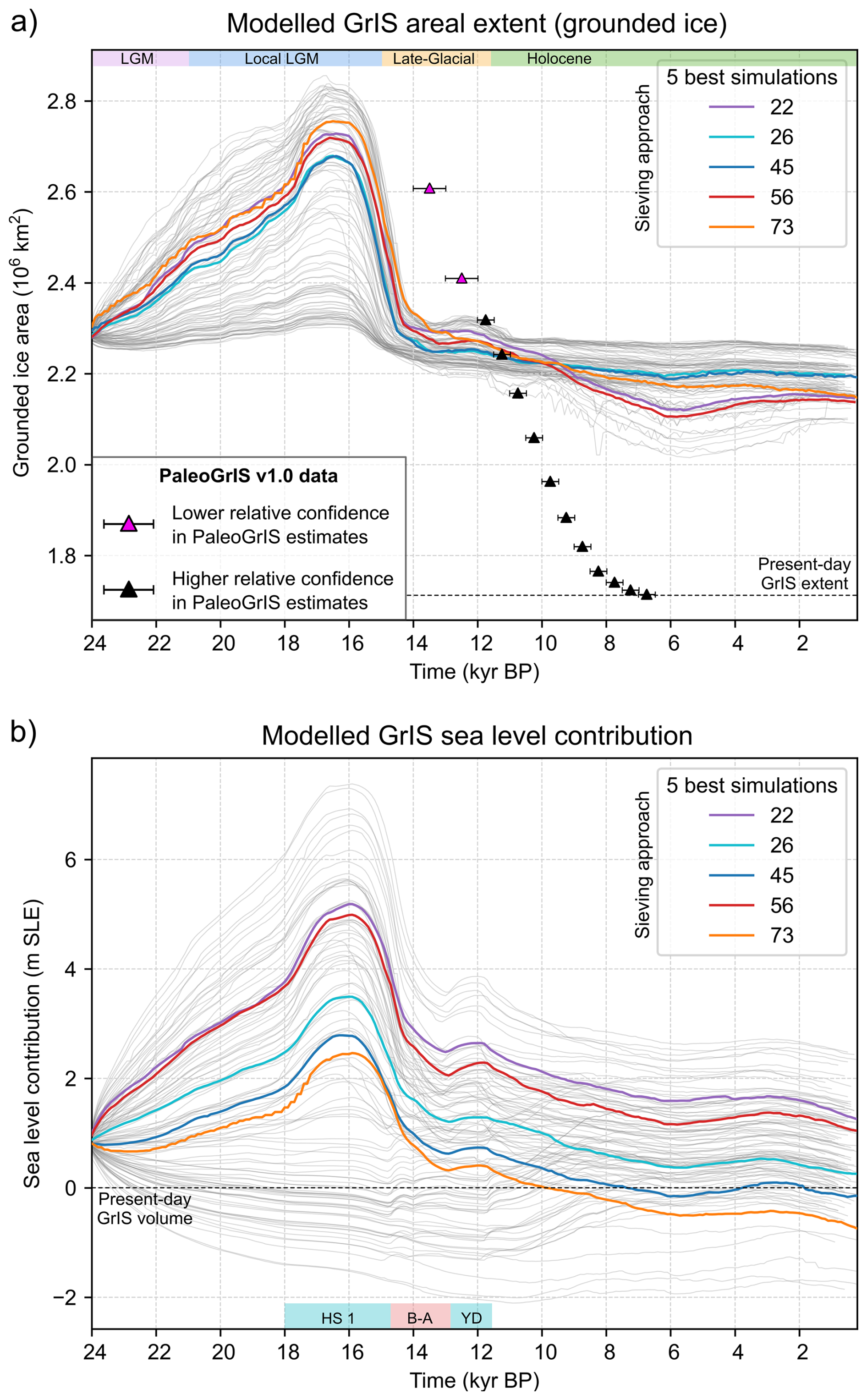
Figure 10 Modelled grounded ice area (a) and ice volume (b) for the 100 transient PISM ensemble simulations of the GrIS (light grey time series) from 24 kyr BP to the PI era (1850 AD). Here, the modelled grounded GrIS volume (in m SLE) is expressed in “sea-level contribution” by subtracting the estimated present-day GrIS volume from our results (7.42 m SLE; Morlighem et al., 2017). GrIS volume calculations exclude ice under flotation computed using the PISM-derived time-dependent flotation criterion. The calculation also excludes the Innuitian ice sheet (IIS), periphery glaciers and icecaps, and any ice thinner than 10 m (after Albrecht et al., 2020). We use ice density, sea water density, and static ocean surface area values of 910 kg m⁻³, 1027 kg m⁻³, and 3.618 × 10⁸ km², respectively. The five overall best-fit simulations (which pass all sieves) are highlighted with thicker coloured time series. The PaleoGrIS v1.0 isochrones data reconstructing the GrIS's former grounded ice extent are shown with triangle symbols on panel a (Leger et al., 2024). Note the GrIS-wide model-data misfit in ice extent apparent here can be misleading as it is spatially heterogeneous and heavily influenced by a few regions concentrating most of the misfit (i.e. NO, NE, and CE Greenland): see Fig. 17. Note the five overall best-fit simulations highlighted here, while passing all sieves, are not the best-scoring simulations at each individual model-data comparison test (see Fig. 12), but rather they score better than other simulations when combining all tests. For instance, their volume during the lLGM (panel b: ∼ 16 kyr BP) is lower and less realistic than values of best-scoring simulations at the local-LGM extent test (see Fig. 12d).

GrIS volume and thickness during the lLGM

lLGM best-fit simulations yield lLGM grounded GrIS volume anomalies (ice above flotation, excluding the IIS and peripheral glaciers) of 6–7.5 m SLE relative to today (∼ 7.42 m, Morlighem et al., 2017) (Fig. 12d). If including ice below flotation, lLGM grounded GrIS volumes for these simulations reach 5.8–6.4 × 10¹⁵ m³. These anomaly values exceed most previous estimates, generally comprised between 2 and 5.5 m SLE (Clark and Mix, 2002; Huybrechts, 2002; Fleming and Lambeck, 2004; Simpson et al., 2009; Khan et al., 2016; Buizert et al., 2018; Bradley et al., 2018; Tabone et al., 2018; Niu et al., 2019; Quiquet et al., 2021; Yang et al., 2022)(Fig. 18). Previous ensemble studies producing LGM-to-present GrIS simulations with model-data comparison (Simpson et al., 2009; Lecavalier et al., 2014) used much coarser grids (15–20 km vs. our 5 km). Certain studies also used ice-sheet models relying exclusively on the SIA (e.g. Zweck and Huybrechts, 2005), and most studies excluded floating ice shelves whose buttressing effect reduces ice-flux and increases grounded ice thickness (Pritchard et al., 2012). Each of these studies also use different climate/ocean forcings and ice flow approximations, and those nudging the model to a specific ice extent may use different data-informed lLGM masks. Together, these differences may help explain the higher volumes obtained in our results. We further note that the study by Yang et al. (2022) model lLGM GrIS sea-level contributions of 2.5 ± 0.25 m SLE (vs. 6–7.5 m in this work), despite also using PISM and a 5 × 5 km model resolution (Fig. 18). This large discrepancy highlights the potent role of differences in input forcings and model parameterisations, and the importance of constraining them through wide parameter space explorations and quantitative model-data comparisons. Indeed, LGM-to-present GrIS simulations by Yang et al. (2022) were not constrained by any observations, and we find many of our ensemble simulations with lower scores at the local-LGM extent test matching their reported lLGM sea-level contributions (Figs. 10, 12).

It can also be challenging to directly compare previously reported GrIS LGM sea-level contribution estimates as different methods are used to compute this number (Albrecht et al., 2020). Studies use different present-day GrIS volume estimates, ice and ocean water densities, global ocean areas, and do not always exclude floating ice nor ice under flotation using a time-varying relative sea-level. However, we believe our workflow follows a method close to that of Lecavalier et al. (2014) when reporting lLGM volumes of the Huy3 model, which is constrained by observations. That model's ratio of grounded GrIS volume (in 10¹⁵ m³ unit) to areal extent (in 10¹² m² unit) during the lLGM (∼ 16.5 kyr BP) is ∼ 1.73 (see Fig. 15 in Lecavalier et al., 2014). In comparison, our five overall best-fit simulations (which pass all sieves) produce ratios of 2.10–2.25, thus 20 %–30 % higher. Our best-fit simulations produce a much thicker lLGM GrIS than the Huy3 model, despite modelling LGM GrIS summit elevations comparable to the present-day ice sheet (Fig. 14). We hypothesise that previous modelling studies may have underestimated the thickness, surface slope, and volume of the grounded GrIS during the lLGM, although we acknowledge this will require more testing in future work.

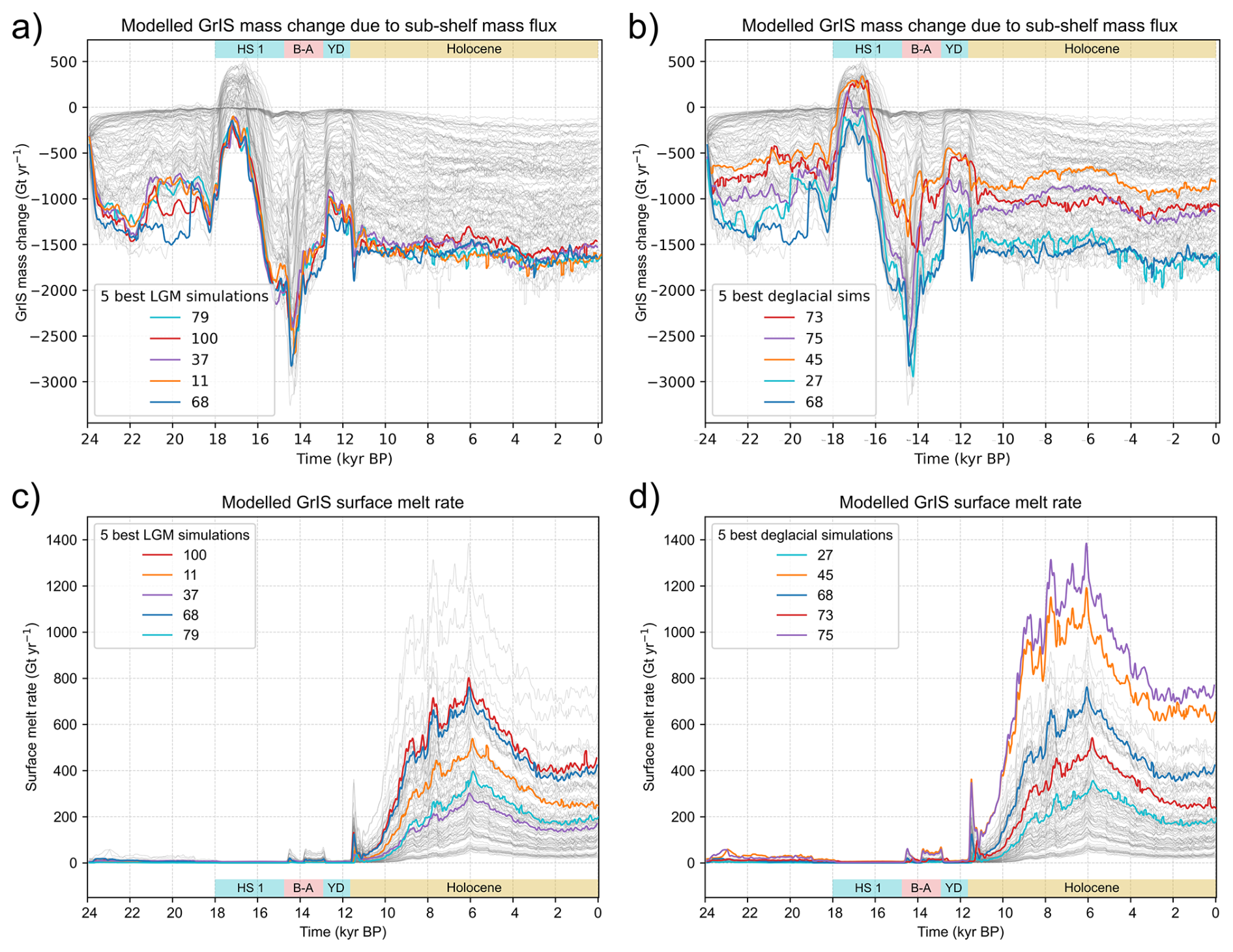
Figure 11 Time series of modelled annual rates of GrIS mass change due to sub-shelf mass flux (a, b), and of modelled GrIS-wide surface melt rate (c, d), for our five best-scoring ensemble simulations at both the local-LGM extent test (a, c) and the deglacial extent test (b, d), highlighted by thicker coloured lines. Data from all other ensemble simulations are shown with thin, light grey lines.

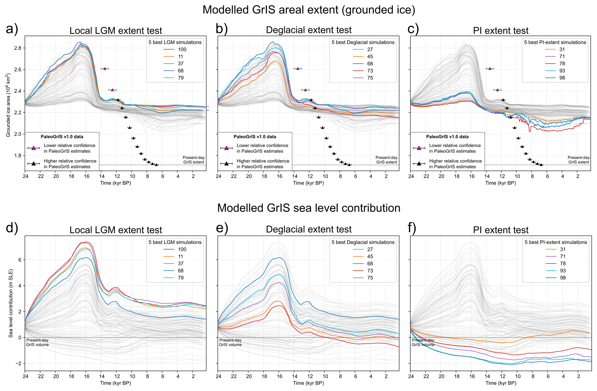
Figure 12 Modelled grounded ice area (a–c) and volume (in m SLE, expressed as sea-level contribution; d–f) for the 100 ensemble simulations (light grey time series). The five best-scoring simulations at each of our three model-data comparison tests are highlighted by thicker coloured time series: (a), (d) for the local-LGM extent test, (b), (e) for the deglacial extent test, and (c), (f) for the PI extent test. Data from the PaleoGrIS v1.0 isochrone reconstruction of former GrIS grounded ice extent (Leger et al., 2024) are shown with triangle symbols. Note the GrIS-wide model-data misfit in ice extent apparent here can be misleading as it is spatially heterogeneous and heavily influenced by a few regions concentrating most of the misfit (i.e. NO, NE, and CE Greenland): see Fig. 17.

In our lLGM best-fit simulations, maximum GrIS volume is associated with spatially heterogeneous GIA-induced bed subsidence (Fig. S2). The largest subsidence values, reaching ∼ 500 m below present-day topography, consistently occur in CW Greenland, around Disko Bay and Sisimiut. Three additional regions of pronounced subsidence (∼ 400 m) are also modelled in CE Greenland (inner Scoresby Sund), upper NE Greenland (Danmark Fjord region), and central Ellesmere Island (Fig. S2). The resulting pattern of total isostatic loading (non-local and local components combined) during the lLGM broadly agrees with previous modelling efforts focusing on GIA signals calibrated against relative sea level indicators (e.g. Simpson et al., 2009; Lecavalier et al., 2014; Bradley et al., 2018).

LGM ice geometry at the locations of ice cores

In Southern Greenland, and following modelled flowlines from the location of the DYE-3 ice core, lLGM best-fit simulations produce a notably different ice-sheet geometry during the lLGM than today (Fig. 14). Modelled ice surface elevations at the local summit are ∼ 300–500 m higher than present, despite greater isostatic loading and ∼ 400 m of bed subsidence. Maximum modelled ice thickness in this region is thus ∼ 700–900 m greater than the present-day GrIS (Morlighem et al., 2017). Toward DYE-3, lLGM best-fit simulations also suggest a notable westward migration of the main East/West ice divide by ∼ 100 km relative to today (Figs. 14, 15). If confirmed, such glacial-interglacial ice-divide shifts would have implications for the DYE-3 ice core record (Dansgaard et al., 1982), which may not have remained as close to the GrIS divide as previously thought during Quaternary glacial maxima. Instead, ice from the drill site may have been located further east within the Helheim glacier catchment, where higher flow velocities and stronger layer deformation could induce irregularities in the ice core profile and complicate chronological interpretation (Rasmussen et al., 2023).

In Northwestern Greenland, near the NEEM ice core (Rasmussen et al., 2013), lLGM best-fit simulations model maximum ice thickness and surface elevations ∼ 200–400 m greater than the present-day GrIS (Fig. 14), but no major migration of the main ice divides (Fig. 15). Towards central Greenland and the locations of the GISP2 and GRIP ice cores (Grootes et al., 1993), simulated ice surface elevations during the lLGM are comparable to present (Fig. 14). There, a complex system of multiple ice divide is modelled during the lLGM, with the main East/West divide shifted up to 150 km east of its present location (Fig. 15). In Northern Greenland, near NGRIP (North Greenland Ice Core Project Members, 2004), both modelled ice divide positions and surface elevations remain close to present-day values during the lLGM. Thus, towards both central (GISP2, GRIP) and northern (NGRIP) GrIS summits, model results suggest the lLGM GrIS was not necessarily thicker than today (Fig. 15). A lack of NGRIP summit migration during the LGM was also suggested by the modelling work of Tabone et al. (2024), thus implying a more stable ice divide during glacial-to-interglacial transitions in central and northern GrIS regions than in other regions. However, we must remain cautious regarding results in the NE GrIS region, as our lLGM best-fit simulations substantially underestimate maximum grounded ice extent in this sector (more discussions in Sect. 5.1.).

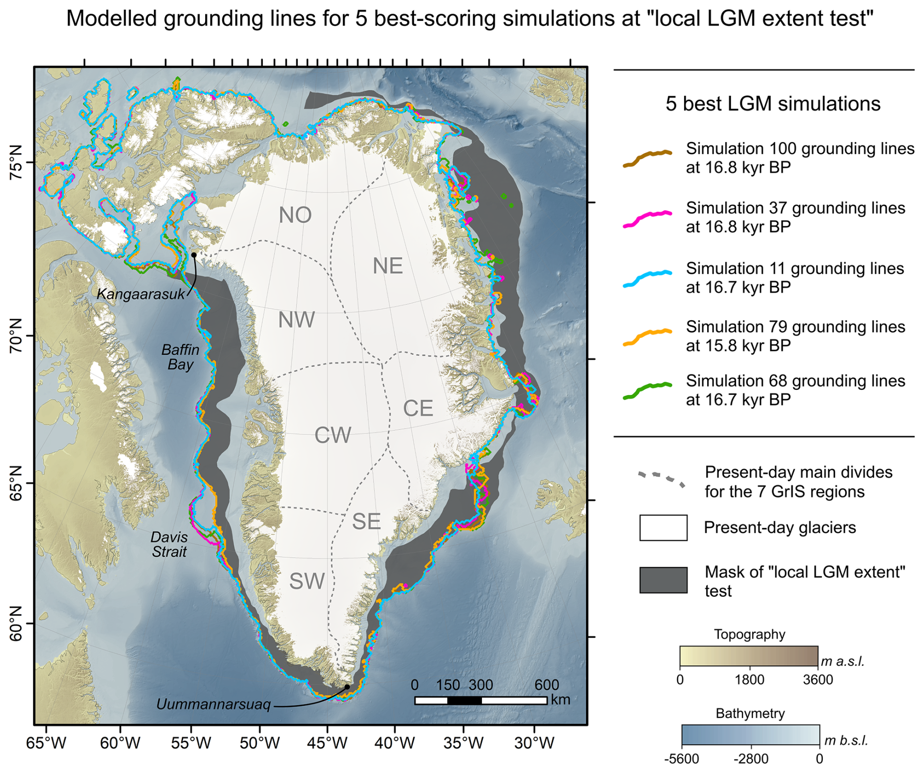
Figure 13 Modelled grounding lines during the GrIS-wide lLGM (maximum ice extent, whose timing is simulation-dependent) for the five best-scoring simulations at the local-LGM extent test. Our division scheme of the GrIS in seven major catchments/regions, used and referred to throughout the text for inter-regional comparisons, is shown with dashed grey lines. Bathymetry and topography data shown in this map are from the 15 arcsec resolution General Bathymetric Chart of the Oceans (GEBCO Bathymetric Compilation Group 2022, 2022). The white mask highlights all present-day ice cover.

GrIS discharge during the lLGM

Our lLGM best-fit simulations produce a faster-flowing GrIS during the lLGM than today. In these runs, areas covered by ice streams (> 800 m yr⁻¹ surface velocities: Bennett, 2003) are 6.8–10.7 times greater during the lLGM than at present (Joughin et al., 2018) (Fig. 16). During the lLGM, our best-fit simulations model GrIS-wide discharge rates that reach 1500–1900 Gt yr⁻¹ (Fig. 19), ∼ 2.8–4.3 times higher than present-day estimates (487 ± 50 Gt yr⁻¹ between 2010 and 2019 AD; Mankoff et al., 2020). These figures are likely underestimates, as our lLGM best-fit simulations do not produce any paleo ice stream in the NE and NEGIS GrIS region despite radar measurement evidence of widespread streaming during the Holocene in this sector (Franke et al., 2022; Jansen et al., 2024). Such higher lLGM discharge rates have implications for past iceberg production, GrIS contributions to Heinrich events, and potential roles in former and future AMOC slowdowns (Ma et al., 2024). However, there are exceptions to modelled localised LGM speedups. In northern Greenland, our lLGM best-fit simulations produce Peterman and Humboldt glaciers flowing slower during the lLGM than today. This likely reflects GrIS–IIS coalescence over Nares Strait during that time, forming an ice dome with low surface slopes and local flow divergence that buttressed and reduced ice flux from upstream regions.

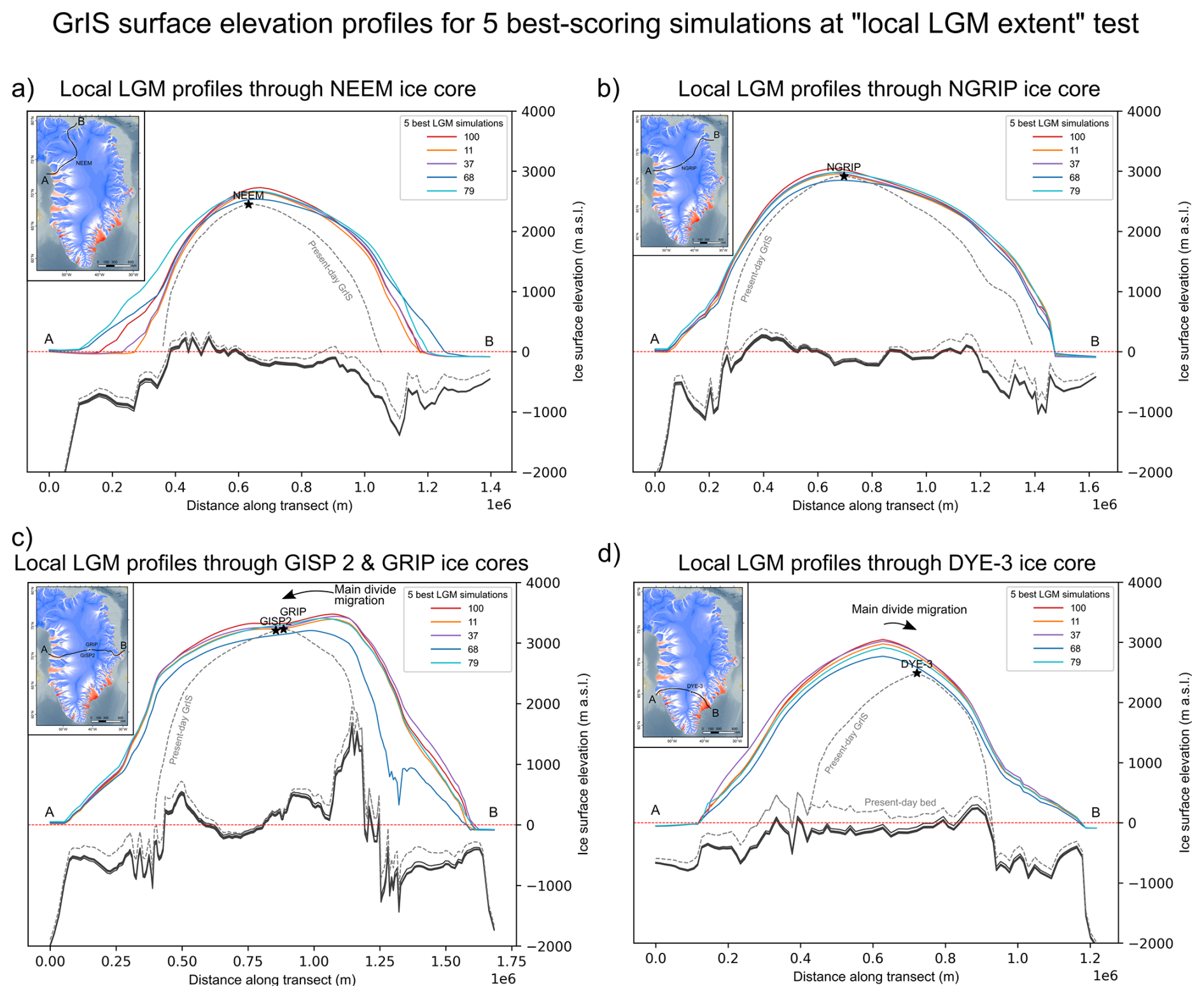
Figure 14 Modelled ice surface and bed elevations during the lLGM extracted across four different transects for our five best-scoring simulations at the local-LGM extent test (thicker coloured lines), and for the present-day GrIS (dashed grey lines). The four transects were drawn following modelled ice flow lines while ensuring to cross the NEEM (a), NGRIP (b), GISP 2 and GRIP (c), and the DYE-3 (d) ice core locations, as shown by the black lines in the inset maps.

3.2 Modelled Greenland Ice Sheet during the last deglaciation

3.2.1 Ensemble-wide trends

Following the lLGM, nearly all ensemble simulations produce rapid, high-magnitude retreat of GrIS margins between 16 and 14 kyr BP, during late HS1 and the Bølling–Allerød warming (B-A; ∼ 14.7–12.9 kyr BP; He et al., 2021a) (Fig. 10). Depending on regions, this abrupt warming raises mean annual and summer air temperatures by 5–12 °C (Fig. 5) and sea surface temperatures by 0.2–3.8 °C (Fig. 6) in our forcing data. In simulations where the GrIS advanced onto continental shelves between 24 and 16 kyr BP, retreat during the B-A causes near-complete deglaciation of continental shelf cover. We find nearly no modelled surface melt across any simulations during the late HS1, B-A warming (16–14 kyr BP), and until ∼ 12 kyr BP (Fig. 11). Instead, modelled margin retreat and mass losses between 16 and 14 kyr BP are associated with more negative (up to tenfold) sub-shelf mass fluxes driven by ocean warming increasing sub-shelf melt rates (Fig. 11). A ∼ 30 % decrease in modelled ice accumulation rates during that time also plays a smaller role. These mechanisms lead to ice sheet thinning of up to 800 m in 2 kyr (Fig. S3). Consistent with Tabone et al. (2018), our ensemble suggests that during late HS1 and B-A warming, ocean forcing drove rapid GrIS retreat and near-total loss of its continental-shelf cover, despite air temperatures remaining too cold to produce surface melt (Fig. 11).

At the ice-sheet scale, ensemble simulations produce little or no GrIS margin re-advance during the Younger Dryas stadial (YD: ∼ 12.9–11.7 kyr BP). In the few runs where grounded margins do re-advance, they recover less than ∼ 3 % of the area lost during deglaciation just prior (∼ 16–14 kyr BP). In the north Atlantic region, the YD was a high-magnitude but short-lived (∼ 1.2 kyr) cooling event, with our forcing data suggesting mean annual temperatures over the GrIS decreasing by ∼ 7 °C relative to 13 kyr BP (Fig. 5). In our simulations, the GrIS is likely still adjusting to major mass and extent loss during the preceding B-A warming. Despite large parameter and climate perturbations between simulations (Table 1), this post B-A inertia combined with the short duration of the YD prevents substantial margin re-advances in most regions. Modelled GrIS volume, however, responds more dynamically to YD cooling, with some simulations recovering up to 8 % of the mass lost between 16 and 13 kyr BP (Figs. 10, 12). During the YD, these simulations display spatially heterogeneous ice-thickness changes: with some thickening of up to ∼ 200 m in CE and Southern GrIS regions, while other areas continue thinning (Fig. S3). Overall, despite strong cooling, our ensemble suggests large GrIS margin re-advances during the YD were unlikely and would have required more sustained forcing. This aligns with the general lack of geomorphological or geochronological evidence for GrIS re-advances during the YD (Leger et al., 2024), and highlights the substantial inertia of the ice sheet following millennial-scale retreat. Contrastingly, numerous peripheral icecaps and glaciers, subject to less inertia due to lower volumes and extents, were more sensitive and did re-advance during the YD (e.g. Larsen et al., 2016; Biette et al., 2020).

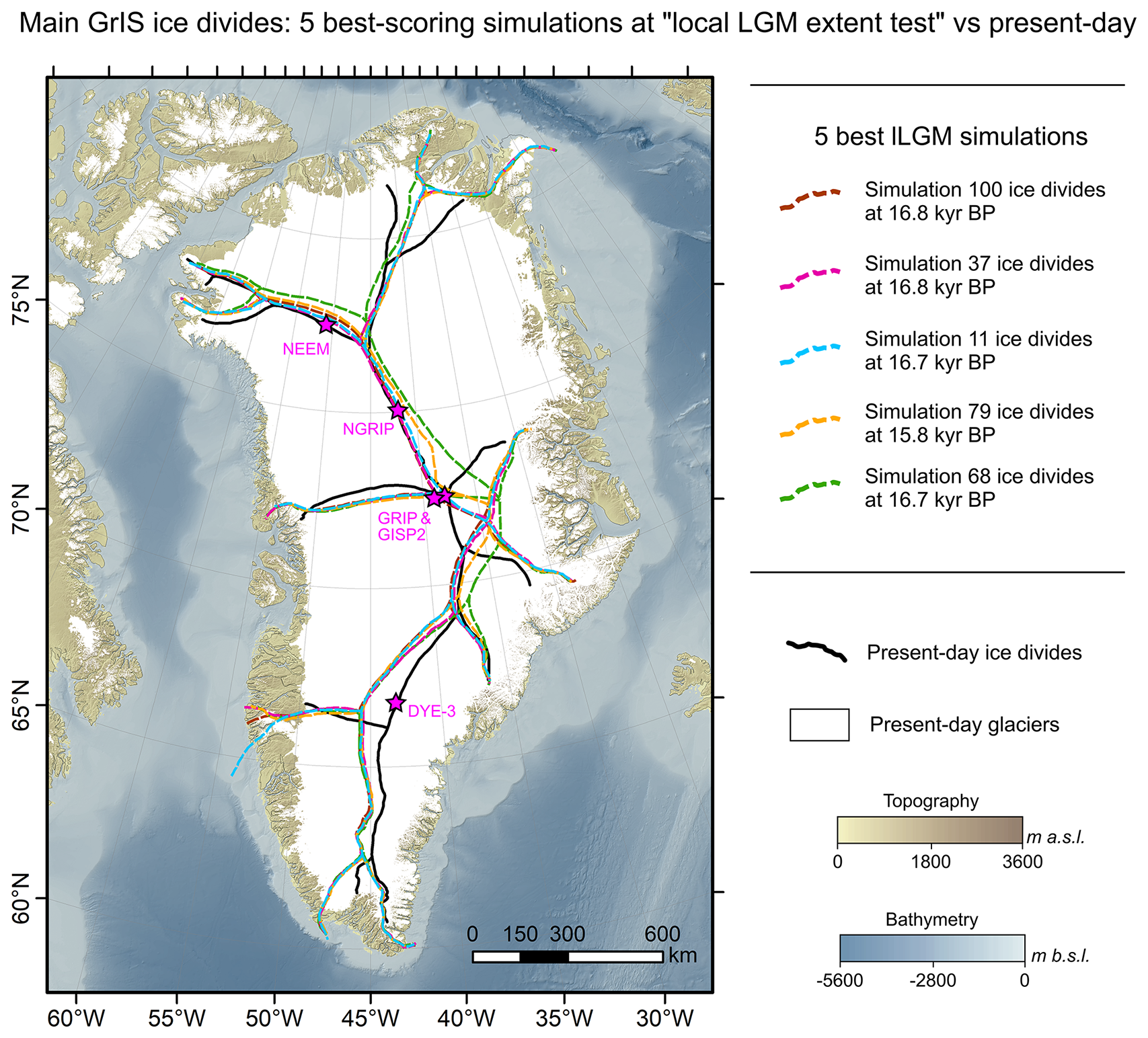
Figure 15 Main GrIS ice divides modelled during the lLGM (maximum GrIS extent, whose timing is simulation-dependent) for our five best-scoring ensemble simulations at the local-LGM extent test (dashed coloured lines). These are compared against the present-day GrIS main ice divides (continuous black line) extracted from surface ice velocity observations (Joughin et al., 2018). The locations of main Greenland ice cores discussed in this study are highlighted by the pink stars. Note the potent offset between the location of the DYE-3 ice core and modelled ice divides during the lLGM (more details in Sect. 3.1.2). Bathymetry and topography data shown in this map are from the 15 arcsec resolution General Bathymetric Chart of the Oceans (GEBCO Bathymetric Compilation Group 2022, 2022).

3.2.2 Insights from deglacial best-fit simulations

In this section, we refer to our “deglacial best-fit simulations” as the five best-scoring ensemble simulations at the Deglacial extent test (Figs. 9, 12).

Deglacial best-fit simulations produce spatially heterogeneous mass-change patterns during the last deglaciation (16–8 kyr BP) (Fig. S3). During the YD stadial (14–12 kyr BP), only small peripheral regions of CE, SE, and SW Greenland gain mass, while other sectors show no change or mass loss. During peak B-A warming (16–14 kyr BP), modelled mass loss is most pronounced in NW, CW, SW, and SE Greenland (Fig. S3). At the ice-sheet scale, deglacial best-fit simulations generate maximum mass loss rates during late HS1 and B-A warming (16–14 kyr BP) reaching ∼ 500–1400 Gt yr⁻¹ (∼ 1–3 mm SLE yr⁻¹) (Fig. 20). By comparison, the GrIS lost an estimated 200–300 Gt yr⁻¹ (0.57 mm SLE yr⁻¹) between 2003 and 2020 AD (Simonsen et al., 2021). Thus, during peak deglaciation (∼ 14.5 kyr BP), best-fit simulations model 2.5–7 times greater mass loss rates than present estimates (Fig. 20). This leads to substantial ice-sheet thinning between 16 and 14 kyr BP in these simulations, especially-pronounced over the CW GrIS (Fig. S3), and causes maximum areal-extent loss rates of 300–450 km² yr⁻¹ (Fig. S4). These modelled area loss rates, primarily linked to ocean forcing, exceed the 170 ± 27 km² yr⁻¹ estimated from the PaleoGrIS 1.0 reconstruction for the ∼ 14–8.5 kyr BP period (Leger et al., 2024). This suggests that grounded GrIS retreat during peak B-A warming was faster than during the YD-to-early Holocene transition, the period covered by most data compiled in PaleoGrIS 1.0, when a larger fraction of the GrIS was land-terminating.

Including Ellesmere Island in our model domain allows reconstruction of coalescence during advance and subsequent unzipping of the GrIS and IIS over Nares Strait during deglaciation. Some deglacial best-fit simulations (e.g. simulation 73) capture this behaviour (Fig. 21). In these runs, most grounded ice over Nares Strait deglaciates between 10 and 8 kyr BP, broadly consistent with geochronological evidence (Jennings et al., 2011) (Fig. 21). For simulations successfully modelling full grounded-ice unzipping of the two ice sheets, final separation (although modelled too late) occurs consistently offshore Peterman glacier near Hall basin, while Kane Basin farther southwest (offshore Humboldt glacier) deglaciates earlier (e.g. Fig. 21).

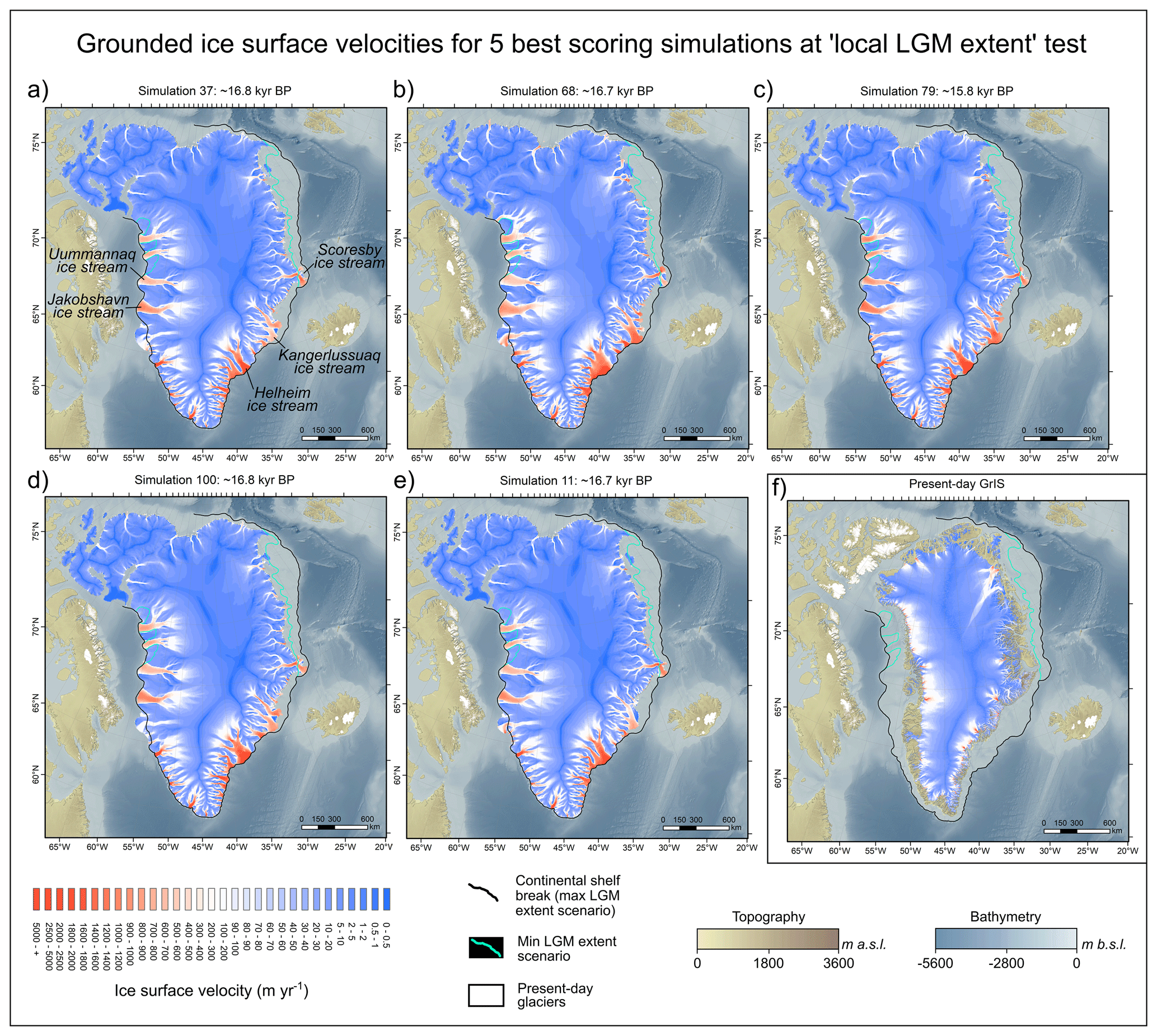
Figure 16 Modelled grounded ice surface velocities during the lLGM (maximum Gris-wide ice extent, whose timing is simulation-dependent) for our five best-scoring ensemble simulations at the local-LGM extent test (a–e), compared with observed present-day GrIS ice surface velocities (f; Joughin et al., 2018). Bathymetry and topography data shown in this map are from the 15 arcsec resolution General Bathymetric Chart of the Oceans (GEBCO Bathymetric Compilation Group 2022, 2022).

3.3 Modelled Greenland Ice Sheet during the Holocene

3.3.1 Ensemble-wide trends

Most ensemble simulations produce a minimum in GrIS areal extent during the mid-Holocene (6–5 kyr BP), before modelling ice-margin re-advances in the late-Holocene and Neoglacial (5 kyr BP–1850 AD). This aligns with empirical reconstructions of Holocene GrIS margin evolution (Funder et al., 2011; Sinclair et al., 2016; Leger et al., 2024). The modelled mid-Holocene minimum in GrIS extent occurs in response to the Holocene Thermal Maximum (HTM), with mean annual and summer surface air temperatures over the GrIS up to 5–7 °C warmer than at the PI (1850 AD) (Figs. 4, 5). In our climate forcing, the HTM peaks at ∼ 6 kyr BP for mean annual temperatures and between ∼ 9–6 kyr BP for summer temperatures, depending on the region. Consistent with the PaleoGrIS 1.0 reconstruction, simulations thus produce ice-sheet inertia causing the ice extent to lag warming cessation and ice-thickness adjustment by centuries to a millennium during the early-to-mid Holocene. Furthermore, all simulations produce a notable ice-sheet volume increase during the late Holocene (3–2 kyr BP) and widespread thinning during the Neoglacial, thus reflecting trends opposite to ice extent (Fig. 10).

During most of the Holocene (8 kyr BP–1850 AD), all simulations produce GrIS mass-change rates remaining below 100 Gt yr⁻¹, despite important variations in climate and SMB parameters between runs (Fig. 20). These rates are lower than present-day mass-loss estimates of 200–300 Gt yr⁻¹ (2003–2020 AD; Simonsen et al., 2021). This result agrees with other GrIS modelling and reconstructions suggesting contemporary and future GrIS mass loss rates are likely unprecedented over much of the Holocene (Briner et al., 2020). Similarly, our ensemble suggests that present-day GrIS discharge rates (487 ± 50 Gt yr⁻¹; Mankoff et al., 2020) are likely unprecedented over the past five millennia (Fig. 19).

3.3.2 Insights from Pre-Industrial best-fit simulations

In this section, we refer to our “PI best-fit simulations” as the five best-scoring ensemble simulations at the PI extent test (Figs. 9, 12).

PI best-fit simulations (e.g. simulation 31) tend to fit the youngest PaleoGrIS 1.0 isochrones (mid-Holocene) better than other ensemble runs (Fig. 12). They produce both a pronounced minimum in grounded GrIS extent at ∼ 5 kyr BP and a margin re-advance between ∼ 5 kyr BP and the PI (1850 AD). During the Holocene minimum, these simulations model some retreat behind present-day GrIS margins, consistent with empirical evidence (e.g. Larsen et al., 2011, 2015), but only in SE and SW Greenland. North of 68° N, no retreat behind present-day margins is modelled except for Humboldt glacier (Fig. S5). Elsewhere, modelled margins remain near or more extensive than present-day margins throughout the mid-to-late-Holocene (5 kyr BP–1850 AD). Simulations with the lowest areal extent during the HTM (e.g. simulation 78; Fig. 12c) produce up to ∼ 100 km retreat behind present-day margins in southernmost Greenland (north of Narsarsuaq), before re-advancing to present-day extents by 1850 AD. Although this may well be an overestimation, our modelling suggests such a retreat magnitude behind present-day margins (∼ 100 km) in response to the HTM cannot be fully ruled out in certain regions. This behaviour is correlated to, and likely caused by, PI best-fit simulations presenting both positive (> +1.5 °C) and negative (< 40 % of original) temperature and precipitation offsets, respectively (Fig. 24).

Within PI best-fit simulations, simulation 31 best reproduces present-day ice thickness (Morlighem et al., 2017) and surface velocity (Joughin et al., 2018) (Figs. S6, S7). The remaining four best-fit simulations underestimate PI GrIS volume (Fig. 12). Even in simulation 31, ice thickness is underestimated in the GrIS interior (up to ∼ 600 m) and overestimated at the margins, whilst modelled ice surface velocities are generally lower than present-day observations (Joughin et al., 2018). This is likely due to underestimated GrIS thickness towards its interior, which reduces ice surface slopes and driving stresses (Figs. S6, S7, S13). The most notable examples are NEGIS and Jacobshavn Isbrae, where the present-day GrIS flows more than 200 m yr⁻¹ faster than simulation 31 during the PI. Therefore, PI best-fit simulations fail to reproduce the particular dynamics of NEGIS. In SE Greenland, however, simulation 31 produces faster-flowing ice in several regions (by more than 200 m yr⁻¹). Interestingly, that is also the case for the terminus of Humboldt glacier (Fig. S7).

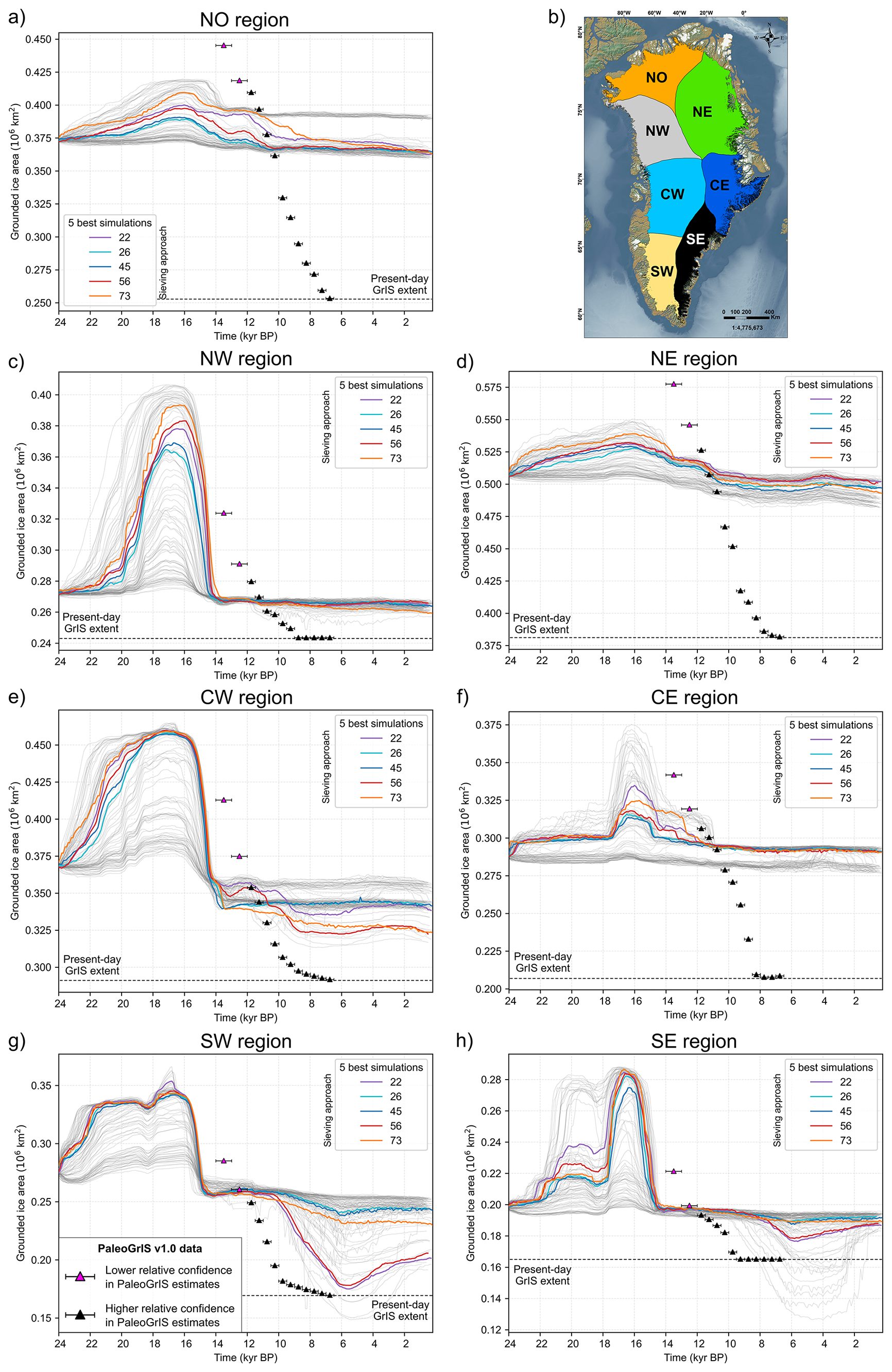
Figure 17 Time series of modelled grounded GrIS extent for our five overall best-fit simulations (which pass all sieves, highlighted by thicker coloured lines) for each of the seven main GrIS regions (a, c–h) whose locations are shown by the inset map on (b). Data from the PaleoGrIS 1.0 ice-extent reconstruction (Leger et al., 2024) are shown with triangle symbols. Data from all other ensemble simulations are shown with thin, light grey lines.

4 Insights from model-data comparison

4.1 Model agreement with empirical data

When compared against the PaleoGrIS 1.0 ice extent reconstruction (Leger et al., 2024), all ensemble simulations underestimate grounded GrIS retreat during the last deglaciation, missing at least 30 % (∼ 0.5 million km²) of the ice-sheet-wide retreat signal (Figs. 10, 12). While more consistent with PaleoGrIS 1.0 during late HS1 and B-A warming (16–14 kyr BP), modelled retreat rates and magnitudes remain too low during the early-to-mid Holocene (12–8 kyr BP). These model-data misfits occur across all simulations despite parameter and climate perturbations (Figs. 10, 12). In addition, the onset of modelled GrIS retreat occurs ∼ 2 kyr earlier than suggested by PaleoGrIS 1.0 (Fig. 10). However, the 14–12 kyr BP PaleoGrIS 1.0 isochrones are limited by data scarcity and timing uncertainties associated with offshore samples, whose radiocarbon dating is complicated by high-latitude marine reservoir effects (Leger et al., 2024). Thus, time ranges of oldest PaleoGrIS 1.0 isochrones should be interpreted with caution. Alternatively, as our results show the onset of modelled GrIS retreat during late HS1 and B-A is primarily controlled by sub-shelf melting (see Sect. 3.2.1.), this offset in retreat timing may also reflect uncertainties and biases in the SST reconstruction (Osman et al., 2021; Fig. 6) used as ocean temperature forcing (see Sect. 5.1. for more discussion).

When analysing model-data agreement at the regional scale, we find that model misfits with the PaleoGrIS 1.0 reconstruction are spatially heterogeneous (Figs. 17, 21, 22). Overall best-fit simulations (which pass all sieves) generally agree better with the PaleoGrIS 1.0 reconstruction during both the lLGM extent and Lateglacial-to-mid-Holocene deglaciation in NW, CW, SW, SE Greenland, and the Kangerlussaq outlet glacier sub-region (CE Greenland), relative to other regions (Fig. 17). Even in these better-fitting areas, best-fit simulations underestimate grounded GrIS retreat magnitudes, but often by less than 50 km. Smaller-scale exceptions occur in the Nuuk fjord and Sisimiut regions, where ice-extent misfits reach 70–90 km depending on the simulation and time period analysed (Figs. 21, 22).

In NO, NE, and CE Greenland (north of 70° N), we find larger model-data misfits in GrIS margin extent and retreat rates (Fig. 17). Although simulations passing all sieves fit PaleoGrIS isochrones well during the 12–11 kyr BP interval in these regions, they underestimate grounded ice extent at the lLGM and retreat rates and magnitudes during the Late-Glacial and early-to-mid Holocene (Figs. 17, 21, 22). In J.C. Christensen Land and Knud Rasmussen Land (NO Greenland, > 80° N), for example, best-fit simulations model grounded margins ∼ 200 km too extensive. The Scoresby Sund fjord system (CE Greenland, 70° N) shows the greatest extent misfit, with an underestimated margin retreat closer to ∼ 230 km, at maximum. Underestimation also remains high (∼ 90–160 km) along the NE Greenland coast, except for the Nioghalvfjerdsbrae (“79N glacier”) and Zachariæ Isstrøm glaciers, where modelled grounded margins agree well with PaleoGrIS 1.0 isochrones through the early-to-mid Holocene (∼ 11–6.5 kyr BP) (Figs. 21, 22).

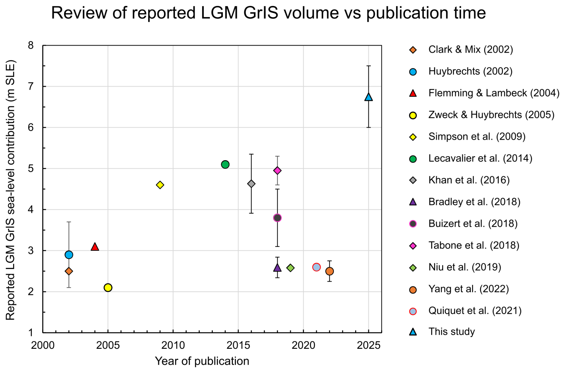
Figure 18 Review of previously modelled and/or reported GrIS volumes during the lLGM (in m SLE, expressed as “sea-level contribution”) plotted against year of study publication, and compared against this study's estimates (blue triangle data point). Note that datapoints lacking error bars relate to when no range or uncertainty was reported in original studies.

Table 2 Ensemble-varying parameter values for the five overall best-fit simulations (which pass all sieves). n/a: not applicable.

Although we use only grounded ice extent data for model-data comparison and scoring, our results can also be evaluated against other empirical datasets. For instance, we compare modelled surface ice elevation change between 8 kyr BP and 1850 AD at four Greenland ice core sites (GRIP, NGRIP, DYE-3, and Camp Century) with δ¹⁸O-derived Holocene thinning curves (Vinther et al., 2009; Lecavalier et al., 2013) (Fig. 23). These curves provide a mean to check whether modelled GrIS thinning rates align with with ice-core data. We find that, despite showing differences in thinning magnitudes and trends, all best-fit simulations (which pass all sieves) produce thinning signals within the 1σ uncertainty bands of the thinning curves for more than 80 % (100 % for NGRIP) of the time period analysed (8–0 kyr BP). One exception is simulation 22 which, at the GRIP site, produces a mid-Holocene elevation offset relative to PI that remains above the upper 1σ limit for ∼ 2.2 kyrs (Fig. 23). By contrast, at DYE-3, simulation 22 matches better than the other best-fit simulations, capturing a higher thinning rate between 8 and 6 kyr BP. All five simulations slightly underestimate the higher thinning rate estimated at Camp Century between 8 and 6.5 kyr BP, a misfit also seen in previous modelling work (e.g. Huy3 model; Lecavalier et al., 2014). Overall, although our ensemble was not scored against thinning curves, best-fit simulations generally reproduce thinning signals within their uncertainties between 8 kyr BP and PI (Fig. 23). This suggests that GrIS simulations constrained by model-data scoring against ice-extent reconstructions tend to also yield realistic Holocene thinning histories. However, while some ensemble members clearly disagree with the thinning curves (Lecavalier et al., 2013), most of the ensemble remains within their 1σ uncertainty bands (Fig. 23). It must also be noted that while we here focus on the 8–0 kyr BP interval, GrIS thinning histories during the early Holocene (12–8 kyr BP) are known to be more challenging to both (i) replicate in models and (ii) correct for in original ice-core derived data (Lecavalier et al., 2017; Tabone et al., 2024). This is due to the demise of the LIS and IIS and unzipping from the GrIS during this interval, and the important impacts of these events on GrIS thinning and bed isostatic adjustment.

We find simulations passing all sieves model temperate basal ice over the vast majority of the GrIS throughout the entire simulation time, from 24 kyr BP to 1850 AD (Figs. S8, S9). However, persistent cold-based regions are modelled towards the ice-sheet's periphery in NO, NE, and CE Greenland. Although basal temperature is amongst the most uncertain model output variables, these results coincide with cosmogenic nuclide inheritance signals, found to be significantly higher for erratic and bedrock samples from NO and NE Greenland regions (Søndergaard et al., 2020; Larsen et al., 2020). These high nuclide inheritance signals observed in northern GrIS regions have often been attributed to a cold-based, non-erosive ice sheet during the lLGM and possibly throughout the last deglaciation (Søndergaard et al., 2020). Therefore, our model results are somewhat coherent with this hypothesis.

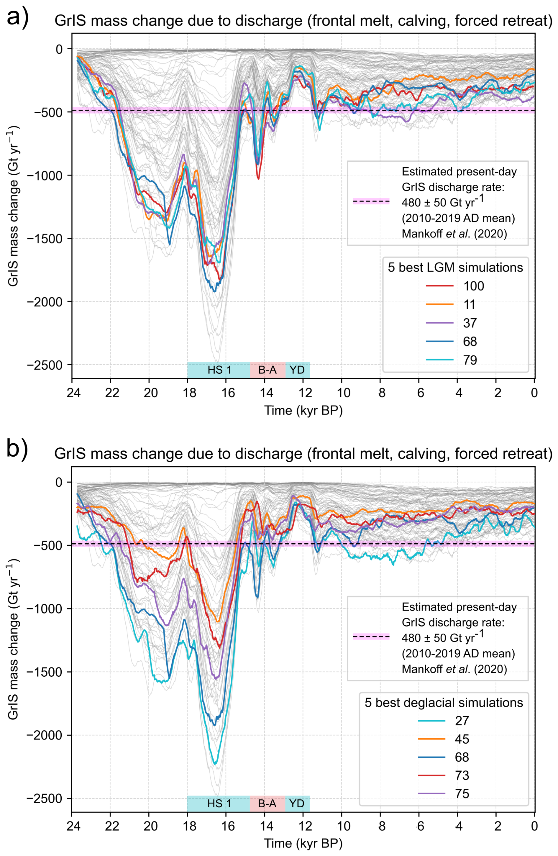
Figure 19 Time series of modelled GrIS mass change due to ice discharge for our five best-scoring ensemble simulations at both the local-LGM extent test (a) and the deglacial extent test (b), highlighted by thicker coloured lines, and compared with an estimated present-day GrIS ice discharge rate (Mankoff et al., 2020). Data from all other ensemble simulations are shown with thin, light grey lines.

4.2 No perfect ensemble simulation

Our model-data comparison scheme yields different sets of five best-fit simulations for each of the three tests, indicating no single simulation consistently matches empirical data across the full 24–0 kyr BP period and all GrIS regions (Fig. 12). Instead, specific ensemble runs must be selected to address research questions on particular time periods or Greenland regions. Consequently, producing a high-resolution (≤ 5 km) LGM-to-present GrIS simulation that is both consistent with physics and in spatially/temporally homogeneous agreement with a detailed empirical reconstruction such as PaleoGrIS 1.0 remains a major challenge.

More specifically, we find that deglacial extent and local-LGM extent test scores are positively correlated (Fig. S10). Simulations that better match data during the lLGM tend to also fit better during the deglaciation, as continental shelves must first be ice-covered to subsequently deglaciate (Fig. 9). However, both the deglacial extent and local-LGM extent test scores are negatively correlated with PI extent test scores: simulations performing well during the lLGM and deglaciation tend to reproduce the PI GrIS extent less accurately, with few exceptions (Fig. S10). This occurs because many simulations fail to produce significant GrIS advance or retreat before the Holocene, instead remaining near the present-day extent throughout (Fig. 12), and thus scoring higher at the PI extent test. This highlights the importance of chronologically ordered sieving across multiple model-data comparison tests when isolating best-fit simulations. Indeed, this prevents overrating a simulation that produces a better PI (or present-day) ice-sheet state, but for the wrong reasons. More generally, this highlights that model initialisations successfully reproducing present-day GrIS geometries are not guaranteed to be ideal initial states for forward modelling, as they may not capture the transient longer-term ice-sheet behaviour, inertia, and memory inherited from the last glaciation and subsequent retreat.

4.3 Are certain parameter values better than others?

We here analysed ensemble-varying parameter values (n=10) for the five best-scoring simulations at each of our three model-data comparisons tests (Figs. 9, 24, Table 1), and find the following:

Three out of 10 ensemble-varying parameters, i.e. the precipitation offset, air temperature offset, and flow law enhancement factor (Table 1), show clustering in best-fit parameter values, meaning specific values may yield better model-data fit (Table 2, Fig. 24). Here, a “cluster” is defined when parameter values of the five best-scoring simulations at each test (Table 2) span less than 50 % of the original sampled parameter range (Table 1). For two ensemble-varying parameters, i.e. the precipitation offset and flow law enhancement factor, values leading to better model-data fit appear test-specific and thus time-dependent. For instance, flow law enhancement factors lower than 1 may lead to better model-data fit in GrIS extent during the lLGM (Table 2, Fig. 24), suggesting maximum expansion is better captured when modelling a GrIS with harder, less deformable, more viscous ice (or lower impurity contents) than modelled by default flow law constants (E=1, n=3). However, this may also represent a compensating adjustment from our modelled ice temperatures, which are warmer (thus possibly resulting in too soft ice) and produce more widespread warm-based conditions over greater proportions of the GrIS than most other GrIS models (e.g. Tabone et al., 2024; MacGregor et al., 2022) and this across all best-fit simulations (e.g. Figs. S8, S9). Parameter clusters further suggest that better fit requires 1.3–2 times higher precipitation during the lLGM and deglacial periods, but 2–5 times lower precipitation during the PI (1850 AD), compared to our default climate forcing (Table 1, Figs. 4, 5, 7, 24). However, due to complex parameter interactions and the simplicity of our SMB parameterisation (PDD), such trends may not necessarily indicate input climate biases but instead hide impactful misrepresentations of ice dynamics and/or boundary conditions, precluding definitive interpretations linked to individual model parameters.

For seven out of 10 ensemble-varying parameters (affecting SMB, yield stress, sliding, or calving), no best-fit clusters were identified, indicating that better model-data fit can occur with highly variable parameter values spanning > 50 % of the sampled ranges (Tables 1, 2, Fig. 24). This suggests that: (i) these seven parameters may not strongly impact the transient evolution of grounded GrIS extent; or (ii) interactions between them may be more impactful than individual parameter perturbations; or (iii) detecting best-fit clusters for these parameters may require a larger-than-100-simulation ensemble and a broader exploration of the parameter space. These findings support the use of ensemble approaches when attempting to match paleo-GrIS model simulations with empirical data, as highly diverse parameter configurations can still yield relatively good model-data fit.

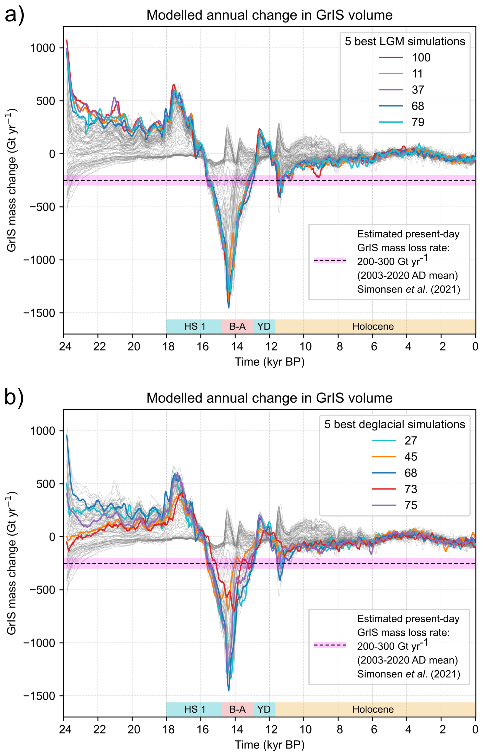
Figure 20 Time series of modelled annual rates of GrIS mass change for our five best-scoring ensemble simulations at both the local-LGM extent test (a) and the deglacial extent test (b) highlighted by thicker coloured lines. The time series are compared against an estimate of present-day GrIS mass loss rate (2003–2020 AD mean; Simonsen et al., 2021). Data from all other ensemble simulations are shown with thin, light grey lines.

5 Remaining misfits: possible causes

As mentioned above (see Sect. 4.1.), model-data misfits in grounded ice extent display strong inter-regional heterogeneities, and are larger in the NO, NE, and CE Greenland regions (Figs. 17, 21, 22). Additionally, simulations passing all sieves (see Methods section) present the most dynamic ice-extent responses through time. They display both higher and lower grounded GrIS extents than ensemble-mean values during the lLGM and mid-Holocene periods, respectively (Fig. 10). This suggests remaining misfits are related to simulations not capturing mechanisms that would enable shorter response times to boundary condition changes and produce higher-amplitude transitional advance and retreat phases. In the following sections, we discuss in more detail the possible mechanisms leading to remaining misfits by dividing them into: (i) misfits in GrIS advance during the lLGM; and (ii) misfits in GrIS retreat during the Late-Glacial and Holocene periods.

5.1 Underestimated LGM advance in NE and NO Greenland

Along the NE Greenland coast (81–71° N), our simulations underestimate the magnitude of grounded ice advance during the lLGM (∼ 17.5–16 kyr BP) (Figs. 9, 13, 16, 17). Studies producing new geomorphological and geochronological reconstructions of GrIS thinning histories (e.g. Roberts et al., 2024) and offshore ice extent (e.g. Arndt et al., 2017; Davies et al., 2022; Hansen et al., 2022) suggest that lLGM grounded GrIS margins reached ∼ 100–200 km further east than our best-fit simulations (Figs. 13, 16).

These model-data misfit during the lLGM may be related to our model initialisation (spinup) procedure reaching a steady-state that does not produce an extensive and/or thick enough GrIS at 24 kyr BP (i.e. the starting time of our transient simulations). This could be due to an inappropriate model parameterisation (e.g. SMB), or to biases in our static input atmospheric or oceanic forcings at 24 kyr BP (see Sect. 2.2.). In the NO and NE regions, the GrIS may require a longer cooling period than the 7.5 kyrs modelled in transient ensemble simulations (between 24 and 16.5 kyr BP) to fully re-adjust to the new parameterisation and switch from a margin location provided by the unique initial state (here close to the present-day GrIS margin) to a margin that needs to reach the mid-to-outer continental shelf. If this is the case, a bias in our model initialisation at 24 kyr BP may be responsible for the underestimated grounded ice advance during the lLGM in NO and NE Greenland.

Another potential source of misfit could be biases in input climate forcing causing either too low precipitation rates, or too high sea-surface temperatures (SST) across NO and NE Greenland. We do not expect biases in air temperature forcing to have a meaningful impact at this stage, as despite conservative ensemble parameter perturbations, we find no PDD-derived surface melt is produced until 12 kyr BP, several millennia after the lLGM and initial deglaciation, due to mean annual and summer temperatures remaining < 0 °C (Figs. 4, 5). We note that during HS1 cooling, input mean-annual SST drops to lower minimum values (−2 to −3 °C) offshore SE and SW Greenland than offshore NE Greenland (−1.5 to −2 °C) (Fig. 6), which may reflect an overestimation of sea-surface temperature forcing in NE Greenland during the lLGM. This 0.5–2 °C drop in SST at around 18–17 kyr BP, which occurs in response to HS1, is a key driver of modelled GrIS expansion during the lLGM, as it is associated with sharp reductions in GrIS-wide sub-shelf melt rates and thus basal mass loss (Fig. 11). A small underestimation in HS1 sea-surface cooling offshore NE Greenland in the order of 1–2 °C may be enough to deter modelled GrIS margins from advancing extensively. This hypothesis may be reinforced by the general lack of SST proxy records used in the data-assimilation scheme of Osman et al. (2021) north of 65° N, offshore Greenland coasts. Biases may also result from our interpolation scheme used for resampling from the nominal 1° horizontal resolution of the original data (Osman et al., 2021), equivalent to a ∼ 20 × 27 km grid offshore NE Greenland, to our 5 × 5 km model grid. This highlights that our experiment is limited by a lack of variation in SST input fields between ensemble simulations. A future experiment using an ensemble-varying parameter introducing spatial and temporal perturbations to the input ocean forcing may help test this hypothesis and possibly increase model-data fit.

Our simulations may also underestimate grounded ice extent in the NO and NE due to too low accumulation rates, largely controlled by our input precipitation forcing. Throughout these regions, iCESM-derived forcing suggests precipitation rates below 20 mm per month during HS1 (Fig. 6). Although iTRACE represents an improvement from the former CESM-derived transient global simulation of the last deglaciation (TRACE-21, Liu et al., 2009), it may still be subject to biases that could misrepresent present-day and former precipitation rates over certain GrIS regions (van Kampenhout et al., 2020; Lofverstrom et al., 2020). In the case of NO and NE Greenland, input precipitation biases in the iTRACE simulation can also originate from the global ice-sheet reconstruction used as forcing within iCESM (ICE-6G: Peltier et al., 2015), which provide slightly incorrect geometries in these regions, impacting the modelled climate used here as input (e.g. Bouttes et al., 2023). More specifically, the ICE-6G reconstruction does not produce a GrIS that extends much beyond the present-day Greenland coastlines, which likely introduces regional biases in CESM simulations due to missing GrIS-atmosphere feedbacks (Bradley et al., 2024). Although we use an ensemble-varying parameter introducing precipitation perturbations of up to +200 % (Table 1), this is not space-dependent and may still be too low over NE Greenland. This may be shown by our lLGM best-fit simulations all displaying precipitation offset values that are clustered towards the upper parameter-range threshold, between 1.8 and 2.0 (Fig. 24). Thus, better model-data scores at the local-LGM extent test could potentially be achieved with precipitation offset values > +200 %. We compared our precipitation forcings with the paleoclimate data assimilation reconstruction of Badgeley et al. (2020), who extended ice-core derived climate reconstructions across Greenland using TRACE-21 (Liu et al., 2009), and also made comparisons with raw data from TraCE-21ka and Buizert et al. (2018)'s reconstruction. This analysis suggests notably lower precipitation rates in our iTRACE-derived climate forcing during HS1, and this in numerous regions across Greenland (Fig. 25b).

Alternatively, our ensemble may be too small to fully explore the full impacts of our climate correction parameters on grounded GrIS extent evolution. As a test, we conducted an additional simulation using default (mid-range) values for all ensemble-varying parameters excluding the precipitation scalar offset (Table 1), here set to 2.0 (+200 % precipitation rate). This test simulation successfully produces an extensive HS1 advance of the grounded GrIS margin offshore NE Greenland, reaching a mid-shelf position. This modelled lLGM advance is more extensive than any ensemble simulations, and suggests our 100-member ensemble did not explore the parameter-space region that produces this specific model response. Therefore, although computationally unfeasible here, running a larger ensemble while keeping perturbed parameter ranges identical may already produce simulations yielding a better model-data fit in ice extent during the lLGM. Alternatively, future experiments running several ensemble waves (e.g. Lecavalier and Tarasov, 2025), with a first ensemble exclusively focused on more widely exploring different climate and ocean forcings with different perturbations schemes, may achieve more data-consistent GrIS LGM-to-present simulations.

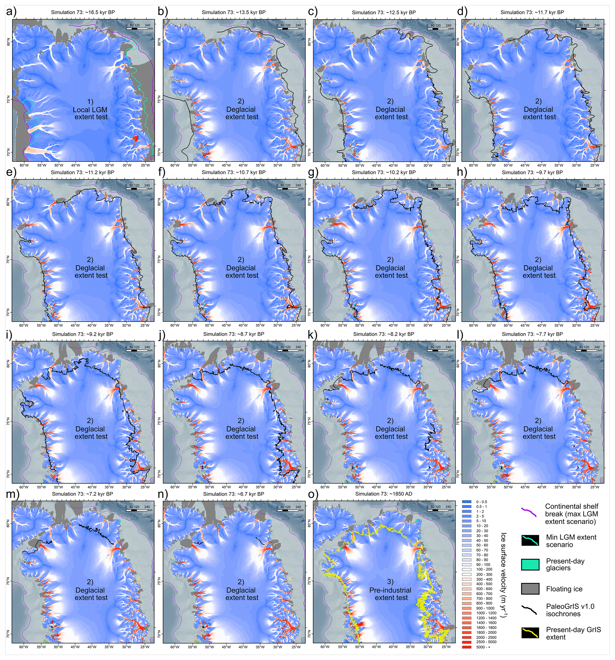
Figure 21 Modelled ice surface velocities of grounded ice for one of the five overall best-fit ensemble simulations (simulation number 73; which passes all sieves), during the lLGM (a), during each of the PaleoGrIS 1.0 isochrone time slices (b–n) (Leger et al., 2024), and during the PI (1850 AD; o). PaleoGrIS 1.0 isochrones for relevant time-slices are plotted with a thick black line. This figure only shows the northern half of the modelled ice sheet for ease of visualisation. The southern half is shown in Fig. 22. Bathymetry data shown in these maps is from the 15 arcsec resolution General Bathymetric Chart of the Oceans (GEBCO Bathymetric Compilation Group 2022, 2022).

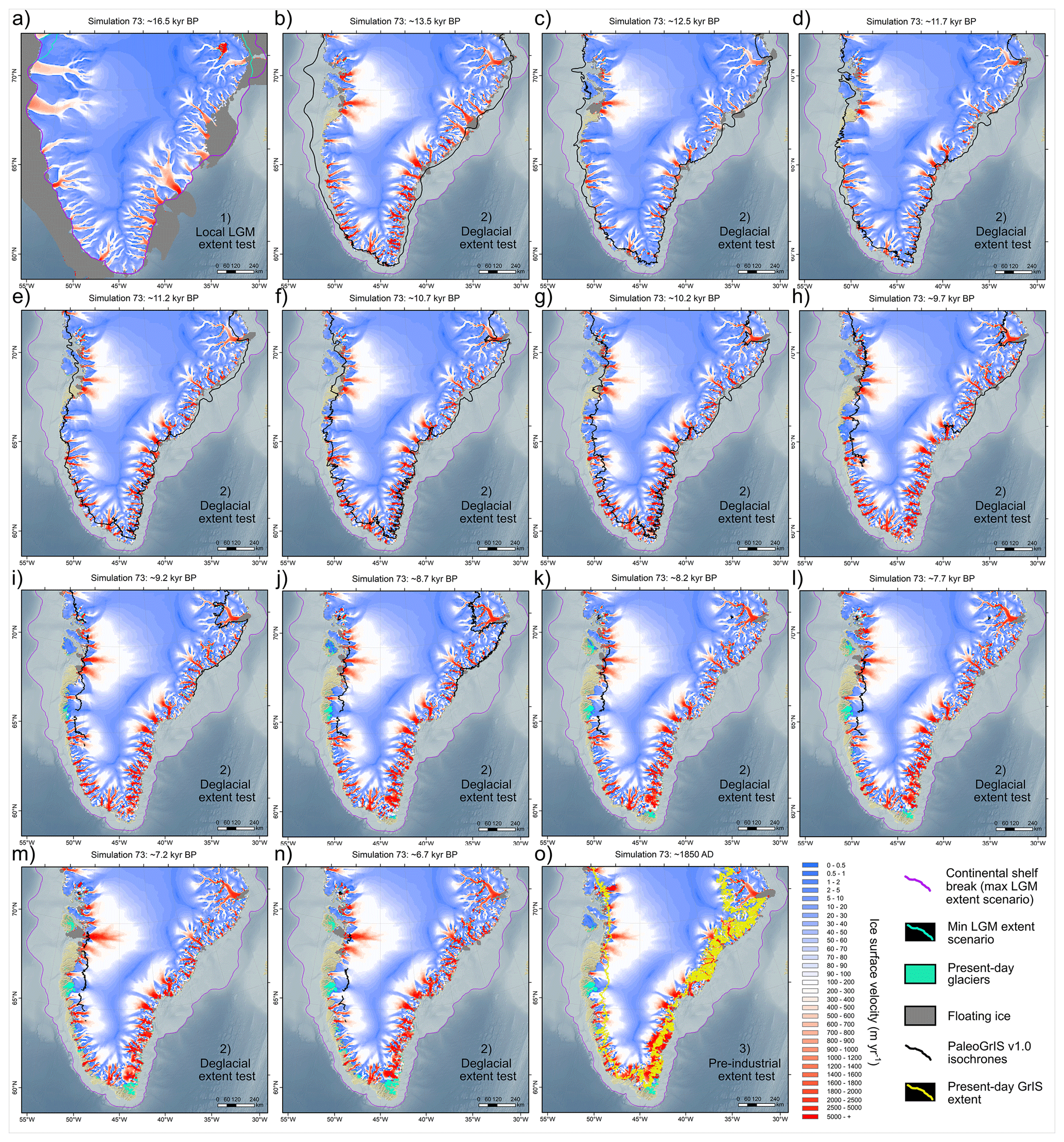
Figure 22 Modelled ice surface velocities of grounded ice for one of the five overall best-fit ensemble simulations (simulation number 73; which passes all sieves), during the lLGM (a), during each of the PaleoGrIS 1.0 isochrone time slices (b–n) (Leger et al., 2024), and during the PI era (1850 AD; o). PaleoGrIS 1.0 isochrones for relevant time-slices are plotted with a thick black line. This figure only shows the southern half of the ice sheet for ease of visualisation. The northern half is shown in Fig. 21. Bathymetry data shown in these maps is from the 15 arcsec resolution General Bathymetric Chart of the Oceans (GEBCO Bathymetric Compilation Group 2022, 2022).

5.2 Underestimated deglacial retreat

We note that the CE and NE GrIS regions, where model-data misfits with PaleoGrIS 1.0 are largest (Figs. 17, 21, 22), present the highest concentration of high elevations and relief (1500–3000 m a.s.l.), steep topographies, and steep-sided fjords in Greenland (Swift et al., 2008; Morlighem et al., 2017). With our 5 km resolution, we find that even towards one of the widest (∼ 20 km) fjords in NE Greenland (Kangerluk Kejser Franz Joseph, 73.2° N; 23.2° W), the topography is heavily flattened (Fig. S14). Summit elevations are underestimated by 30 %–50 %, and average slope along a cross-fjord transect is 40 % and 35 % lower than if using 150 m and 1 km resolution grids, respectively (see Fig. S14). In such rough topographies, a finer model resolution (e.g. 1 × 1 km or lower) would lead to higher ice flux rates (as shown by Leger et al., 2025), and to deeper fjords enabling more water ingress as modelled tidewater glaciers retreat. Both mechanisms would likely enhance modelled GrIS thinning and retreat rates during deglaciation. This is supported by Aschwanden et al. (2016) who, using PISM, better matched observed flow velocities of main present-day GrIS outlet glaciers (e.g. Nuussuup Sermia, Sermeq Kujalleq) using resolutions of 600 and 1500 m, relative to 3600 and 4500 m, the latter causing underestimations of maximum flow velocities by factors of 4–7. Therefore, we hypothesise that coarse model resolution may contribute to our higher relative ice-extent model-data misfits observed in the CE and NE regions during the last deglaciation.

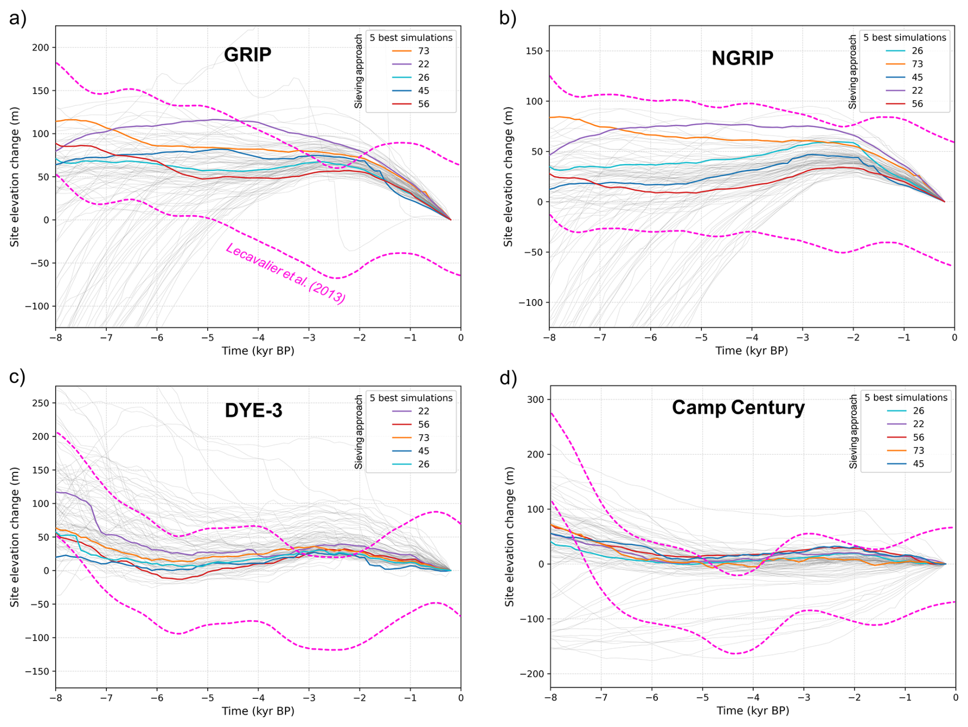
Figure 23 Comparison between ice elevation change modelled by our five overall best-fit simulations (which pass all sieves; thicker coloured lines) and the 1σ uncertainty band of the Holocene thinning curves (dashed pink lines), derived from ice core δ¹⁸O records. Holocene thinning curves were produced by Lecavalier et al. (2013), improving from Vinther et al. (2009) following an elevation correction for thickness changes at the Agassiz and Renland ice caps. Data from all other ensemble simulations from this study are shown with thin, light grey lines.

Larger model-data misfits in the magnitude and rates of GrIS retreat during the Late-Glacial and early-to-mid Holocene in NO, NE, and CE Greenland are also likely associated with biases in our input climate forcing, including possible underestimations of sea-surface and atmospheric warming (∼ 14–6 kyr BP). As mentioned above, biases in iTRACE-derived climate are possible, especially towards the margins of the former GrIS. For instance, an overestimation of the ice thickness and extent reconstruction used as forcing within iCESM (ICE-6G: Peltier et al., 2015) during the last deglaciation in NO, NE, and CE Greenland, would lead to unrealistically high albedo feedbacks impeding the atmospheric warming required to model appropriate GrIS thinning and retreat rates. Our experiment features an ensemble-varying temperature offset parameter (Table 1) with maximum space-independent warming of up to +3.5 °C, along with ensemble-varying snow and ice PDD melt factors that can reach 5 and 12 mm we d⁻¹ °C⁻¹, respectively. However, with important input climate biases in the regions of concern, these perturbations may still underestimate the resulting surface melt during deglaciation (see Fig. 25a, c). We note that a cold temperature bias during the Late-Glacial and early-to-mid Holocene is not supported by comparison against the climate reconstruction (and its associated uncertainty range) of Badgeley et al. (2020), which instead suggests that our forcing produce relatively warm mean annual temperature anomalies towards the GrIS summit and NO, NE, and CE GrIS regions, between 15 and 5 kyr BP (Fig. 25c). On the other hand, this comparison reveals that our iTRACE and iCESM - derived climate forcing results in significantly higher (up to ∼ 100 %) precipitation rates during the entire Holocene towards the GrIS summit and its vicinity, than is obtained in ice-core-data-informed reconstructions from Badgeley et al. (2020) and Buizert et al. (2018) (Fig. 25d). Although the HTM has been shown to likely be associated with higher-than-present precipitation (e.g. Downs et al., 2020), and although our experiment features an ensemble-varying precipitation offset scheme with possible reductions down to 20 % input precipitation, this potential positive bias may be responsible for too high Holocene precipitation in many of our ensemble simulations, thus impeding GrIS retreat in certain regions and causing ice-extent overestimation during the modelled deglaciation but also during the PI (Fig. 25d). Moreover, it is worth noting that CESM has been also shown to overestimate (by < 20 %) present-day snowfall precipitation over the GrIS relative to observations which may also explain our overestimation in ice extent during the PI (e.g. Lenaerts et al., 2020; Fig. 5 therein).

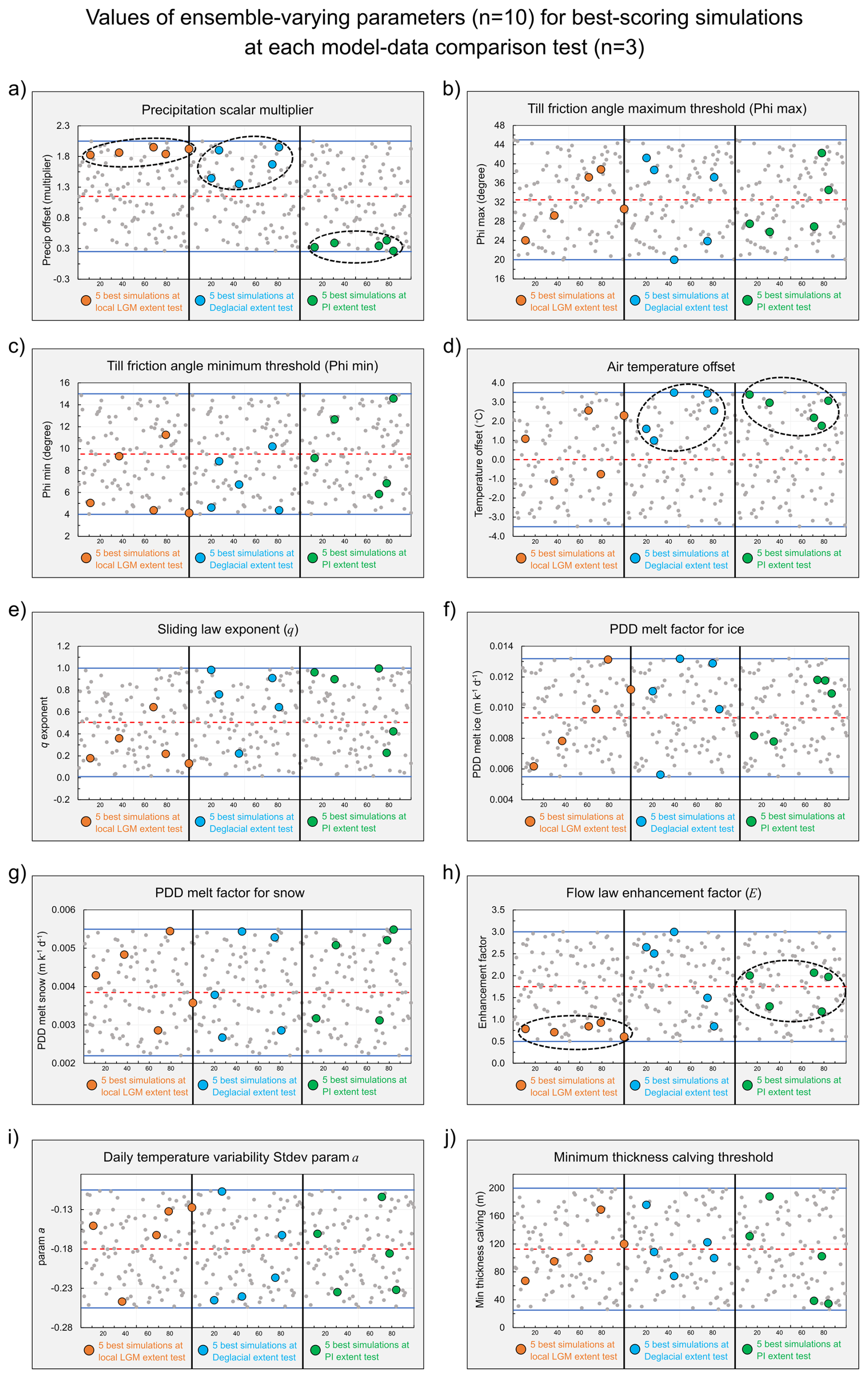
Figure 24 Values of the 10 ensemble-varying parameters for all simulations (n=100, grey dots) and for the five best-scoring simulations (larger coloured dots) at each of the three model-data comparison tests (separated by vertical black lines). Dashed black ellipses (in a, d, and h) highlight best-fit parameter “clusters”, defined as such when the parameter values for the five best-fit simulations (coloured dots) cover a range < 50  % of the parameter value range (highlighted by horizontal blue lines) originally sampled with the Latin Hypercube technique (also see Table 1). All x axes represent ensemble simulation numbers (0–100).

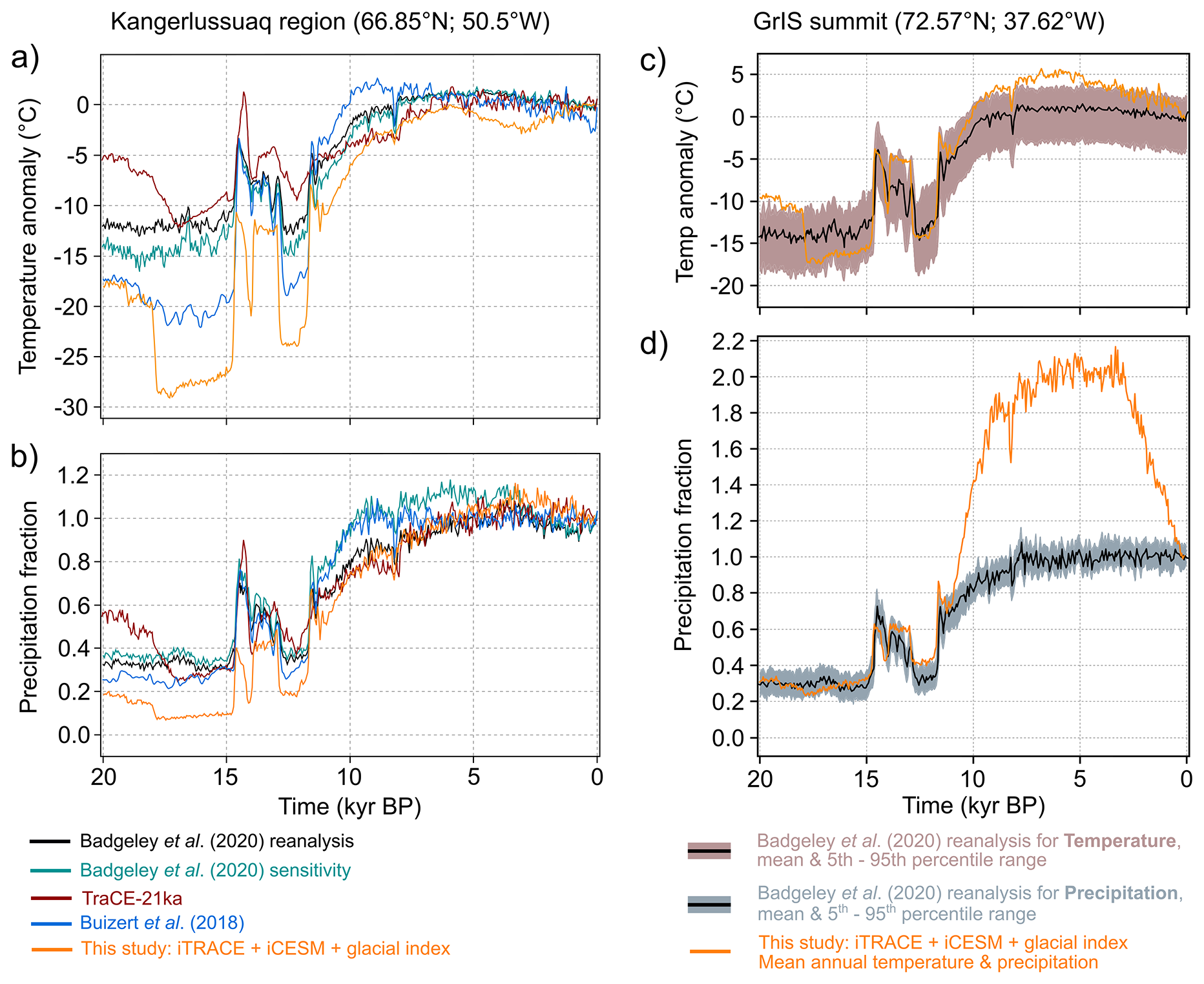
Figure 25 Comparisons between our input mean annual temperature and precipitation forcings (orange time series) with the climate reconstructions of Badgeley et al. (2020), Buizert et al. (2018), and raw TraCE-21ka model output (Liu et al., 2009). More specifically, these panels present the same data as shown in Figs. 8 and 13 in Badgeley et al. (2020). Note that precipitation fractions and temperature anomalies are here expressed with reference to the mean of 1850–2000 AD for all datasets except this study's input climate data (orange), instead expressed with reference to the mean of 1750–1850 AD, caused by our most recent iCESM simulation being 1850 AD.

Alternatively, our ensemble (n=100) may be too small to explore the full impact of these temperature and PDD melt parameter perturbations on modelled GrIS retreat during deglaciation. Furthermore, our SMB parameterisation, based on on a simple PDD scheme (Calov and Greve, 2005), does not capture additional contribution to melting from past changes in insolation forcing, nor certain ablation mechanisms such as sublimation and wind-driven snow layer erosion, nor does it fully capture the elevation feedback between the modelled ice-sheet surface and climate forcing. These missing mechanisms may be important to model deglacial GrIS thinning and retreat accurately at high latitudes (> 75° N), where mean summer air temperatures during the HTM remained close to or below 0 °C (at least in our forcing data) (Fig. 5) (Plach et al., 2019), and where additional summer melt contributions from increased insolation during the Late-glacial and early Holocene were likely important (Robinson and Goelzer, 2014). In future work, the use of SMB energy-balance models incorporating insolation forcing (e.g. dEBM; Krebs-Kanzow et al., 2021) instead of PDD parameterisations would potentially help reduce model-data misfits in GrIS extent during the last deglaciation. Alternatively, the underestimated modelled GrIS retreat in NO, NE, and CE Greenland could be associated with a lower-than-needed ocean temperature increase during the last deglaciation (Osman et al., 2021; Figs. 6, 7) offshore the present-day GrIS. We note that our ice-ocean interaction model does not consider multiple ocean layers, which are important when poorly mixed sub-surface layers of higher temperatures increase sub-shelf melt at depth and towards the grounding line (Lloyd et al., 2023). It also does not consider a seasonal cycle of ocean water temperature change as forcing, which may be important to model the necessary magnitude of deglacial sub-shelf melt in these regions. We also note that, for instance, TrACE-21ka-derived shelf-depth ocean forcing used in Tabone et al. (2024; Fig. S3 therein) reaches above 0 °C (up to 2 °C) towards the NE Greenland outer shelf, between 13 and 8 kyr BP, whilst our SST forcing does not produce values above −1 °C in that region and timeframe.

Today, up to ∼ 16 % of the GrIS is thought to be drained by NEGIS (Hvidberg et al., 2020), a singular ice stream that can prove challenging to model accurately (Smith-Johnsen et al., 2020). In our best-fit simulations, some ice streaming is modelled towards both Nioghalvfjerdsbrae (79N glacier) and Zachariae Isstrom glaciers, throughout the full simulation timespan (e.g. Figs. 16, 21). However, a comparison between our best-fit simulations at the PI extent test and present-day GrIS surface velocities (Joughin et al., 2018) reveals that our model underestimates GrIS flow speeds towards NEGIS (Fig. S7). Our simulations do not capture its singular shape featuring a relatively narrow (< 100 km) and long (>500 km) band of relatively high (> 50 m yr⁻¹) surface velocities nearly reaching the ice-sheet's central East/West divide (Fig. S7). Although uncertainties remain regarding the timing of last NEGIS activation into its present-day configuration, recent evidence suggests it was active in its present form ∼ 2000 years ago (Franke et al., 2022; Jansen et al., 2024), whilst the modelling study of Tabone et al. (2024) suggests that NEGIS may be up to 8000 years old. Due to its significant impact on ice flux of the entire NE GrIS region, modelling an accurate NEGIS configuration throughout the Late-Glacial and Holocene periods would produce higher regional-mean discharge and thinning rates. Over millennial timescales, this may help model greater and more data-consistent GrIS margin retreat rates during deglaciation. This is supported by the results of Tabone et al. (2024) which suggest that an early-Holocene activation of a present-like NEGIS, achieved through highly targeted parameterisation of low basal friction along the ice stream, is crucial to drive deglacial ice thinning over the central and northern GrIS. Therefore, it is likely that not fully reproducing NEGIS may contribute to increasing model-data misfits in NE Greenland relative to other GrIS regions, where ice streams are generally less challenging to model accurately.

6 Conclusions

In this study, we conducted a perturbed-parameter ensemble of 100 PISM simulations of the entire Greenland-Ice-Sheet evolution from 24 000 years ago to the pre-industrial era (1850 AD) at a spatial resolution of 5 × 5 km. Each simulation was quantitatively scored against ice-sheet-wide empirical data of former grounded ice extent and its timing. We here summarize the main findings from this model-data comparison experiment.

• The maximum grounded Greenland Ice Sheet extent, i.e. the lLGM, likely occurred between 17.5 and 16 kyr BP, during Heinrich Stadial 1. At that time, the grounded ice sheet reached an area of between 2.9 and 3.1 million km². During full glaciation, grounded ice likely reached the continental shelf break along the entire Western, Southern, and Southeastern Greenland coasts.

• Our results suggest that between the lLGM and today, the global mean sea-level rise contribution of the Greenland Ice Sheet is between 6 and 7.5 m, a number higher than previous estimates (see Sect. 3.1.2.). During the lLGM, the ice sheet was not necessarily thicker (nor higher-elevated) than today at its summits, towards the GISP2, GRIP, and NGRIP ice core sites. Contrastingly, in Southern and Northwestern Greenland (DYE-3 and NEEM ice cores), the ice sheet was likely up to ∼ 1 km thicker than today, with an ice surface up to ∼ 500 m higher in elevation, thus causing ice divide migrations between full glacial and interglacial periods. These migrations may have important implications for the chronological interpretation of the DYE-3 ice core. During maximum extent, the ice sheet was also flowing faster and was able to discharge up to 5.1 times more ice than today, thus contributing substantially more iceberg and freshwater delivery to the north Atlantic basin than today.

• The Greenland Ice Sheet likely retreated rapidly and extensively during the late Heinrich-stadial 1 and Bølling–Allerød warming events, between 16 and 14 kyr BP. During that time, the grounded ice sheet lost the majority of its continental shelf cover. This rapid demise was likely mainly caused by ocean warming and increased sub-shelf melt, while air temperatures likely remained too cold to generate significant surface melt. During this phase of rapid retreat, the ice sheet may have experienced up to 7 times greater mass loss rates than are currently estimated for the present-day.

• At the Greenland Ice Sheet scale, margin stabilisation and readvances during the Younger Dryas cooling event were likely limited and of low magnitude, as opposed to peripheral glaciers which demonstrated a more dynamic response. We hypothesise this was caused by strong ice-sheet inertia and geometrical/thermal ice memory feedbacks associated with the potent deglaciation experienced just prior, during Bølling–Allerød warming.

• The Greenland Ice Sheet likely reached a minimum in ice extent between 6 and 5 kyr BP, and thus lagged the cessation of Holocene Thermal Maximum warming by a few centuries, and up to a millennium, prior to experiencing late-Holocene and Neoglacial readvance. During the mid-Holocene, our simulations produce up to ∼ 100 km of margin retreat behind the present-day Greenland Ice Sheet, but only south of 68° N.

• While best-fit simulations are in reasonable agreement with the PaleoGrIS 1.0 grounded ice-extent reconstruction in Northwestern, Central-western, Southwestern, and Southeastern Greenland regions, we find larger model-data misfits remain in the Northern, Northeastern, and Central-eastern regions. There, magnitudes and rates of modelled LGM advance and deglacial retreat are both underestimated, when compared to empirical data. This suggests these regions are significantly more challenging to model accurately. We hypothesise these misfits are possibly related to multiple causes including biases from: surface mass balance and ice-ocean interaction parameterisations, input climate and ocean forcings, model resolution due to rougher local topographies, model initialisation, and the difficulty to reproduce the Northeast Greenland Ice Stream.

• No single ensemble simulation could achieve a better relative score at all three chronologically-distinct model-data comparison tests. Instead, we find different simulations and parameter configurations are needed to better match empirical data in certain Greenland regions or during certain millennial-scale events (e.g. the early-Holocene). Thus, producing a physically-sound 3D model simulation that is data-consistent across all Greenland regions since the last glaciation, which would enable accurately capturing the ice-sheet's memory from this key period of environmental change, is still a major challenge. To achieve this, future work may need to employ larger ensembles, more appropriate parameterisations of boundary conditions, data assimilation to reduce biases, higher resolution modelling, and more time- and space-dependent parameter and paleoclimate perturbations.