Historical snow measurements in the central and southern Apennine Mountains: climatology, variability, and trend

This work presents an analysis of historical snow precipitation data collected in the period 1951–2001 in central and southern Apennines (Italy), an area scarcely investigated so far. To pursue this aim, we used the monthly observations of the snow cover duration, number of days with snowfall and total height of new snow collected at 129 stations located between 288 and 1750 m above sea level. Such data have been manually digitised from the Hydrological Yearbooks of the Italian National Hydrological and Mareographic Service. The available dataset has been primarily analysed to build a reference climatology (related to the 1971–2000 period) for the considered Apennine region. More specifically, using a methodology based on principal component analysis and k-means clustering, we have identified different modes of spatial variability, mainly depending on the elevation, which reflect different climatic zones. Subsequently, focusing on the number of days with snowfall and snow cover duration on the ground, we have carried out a linear trend analysis, employing the Theil–Sen estimator and the Mann–Kendall test. An overall negative tendency has been found for both variables. For clusters including only stations above 1000 m above the sea level, a significant (at 90 % or 95 % confidence levels) decreasing trend has been found in the winter season (i.e. from December to February), with −3.2 [−6.0 to 0.0] d per 10 years for snow cover duration and −1.6 [−2.5 to −0.6] d per 10 years for number of days with snowfall. Moreover, in all considered seasons, a clear and direct relationship between the trend magnitude and elevation has emerged. In addition, using a cross-wavelet analysis, we found a close in-phase linkage on a decadal timescale between the investigated snow indicators and the Eastern Mediterranean teleconnection Pattern. For both snow cover duration and number of days with snowfall, such connection appears to be more relevant in the full (i.e. from November to April) and in the late (i.e. from February to April) seasons.

1 Introduction

In recent years, a great deal of attention has been devoted to the study of past snow variability worldwide, mainly in mountain regions. The great interest in this crucial climate variable is motivated by several reasons. The snow, in fact, is a pivotal component of the hydrological cycle and exerts, at the same time, a relevant impact on the energy balance, controlling the land surface albedo. In addition, the snow strongly affects the complex ecosystems of mountain areas, as well as the biogeochemical cycles (e.g. Magnani et al., 2017). Last, the occurrence, as well as the persistence of snow on the ground, is decisive for winter tourism and for several economic activities (for instance, hydropower production). Therefore, when considering the recent climate changes that are posing serious threats to the cryosphere and mountain regions (e.g. Mote et al., 2018; Kotlarski et al., 2022), it is crucial to recover and analyse historical long-term time series of snow data to assess the variability and tendencies.

In the last few decades, satellite observations and climate model reanalyses have offered new opportunities for built-up snow climatologies worldwide (e.g. Bormann et al., 2018; Olefs et al., 2020), especially in regions in which the availability of in situ data is scarce or totally absent. However, it should be noted that remote sensing could provide information about snow cover at an adequate resolution for reliable climatological analyses only for the last 20 years, after the deployment of the Moderate Resolution Imaging Spectroradiometer (MODIS) constellation (Fugazza et al., 2021; Gascoin et al., 2022; Dumont et al., 2024). On the other hand, as highlighted by Vernay et al. (2022), the reliability of the reanalyses data can be adversely affected by the low spatial resolution and by the rough representation of several sub-grid processes, such as the orographic precipitation and the local thermal inversion in mountain valleys. The latter can strongly condition local nivometric regimes, particularly in mountainous areas characterised by complex orography. For such reasons, despite their well-known weaknesses (Notarnicola, 2020), the ground-based historical observations can be still considered a cornerstone for studies searching for evidence of past snow variability. Accurate in situ snow measures open the chance to conduct an in-depth analysis of the climate change impacts in mountain areas and their relationship with the altitude, especially when they can be coupled with high-quality and homogenised temperature and total precipitation measurements (Beaumet et al., 2021). In addition, the ground observations can be considered an invaluable benchmark to validate satellite and modelled snow data.

In the large body of available scientific literature, snow has been investigated employing different parameters, namely the snow depth (hereafter HS), the height of new snow (hereafter HN), the snow water equivalent, the snow cover area, the snow cover duration (hereafter SCD), and the number of days with snowfall (hereafter NDS). Note that in the literature, SCD generally indicates the number of days with snow cover on the ground during a given period, whereas the NDS parameter represents the number of days, in a determined time interval, on which the amount of fresh snow reaches a determined threshold (usually, 1.0 cm).

Focusing on the central Mediterranean region, which can be considered a key area for the study of climate changes, mainly due to its complex meteorological regime and its challenging topography, a lot of research has been done in the Alpine region (Marty, 2008; Terzago et al., 2010; Valt and Cianfarra, 2010; Marty and Blanchet, 2012; Scherrer et al., 2013; Terzago et al., 2013; Marcolini et al., 2017b; Matiu et al., 2021; Colombo et al., 2022; Bertoldi et al., 2023; Colombo et al., 2023). In this area, in fact, there is a great availability of snow climatological time series, some of them stretching back to the late 18th century (Leporati and Mercalli, 1994). Although it is clearly challenging to draw a coherent picture regarding changes in Alpine nivometric regimes since the trend direction and significance are highly dependent on the considered time period, a general decreasing tendency has been found for SCD in the period 1972–2006 (Bartolini et al., 2010), as well as in HS for the period 1971–2019 (Matiu et al., 2021).

The Apennine region, despite having a good heritage of old snow data, has been poorly investigated up to now. The peer-reviewed literature for this area counts only few recent works (Petriccione and Bricca, 2019; Diodato et al., 2022; Capozzi et al., 2022; Annella et al., 2023), which presented evidence based on a single or a few climatological time series. These studies highlighted a generally negative tendency in snow for different indicators, except for the last 20 years, in which a recovery of SCD, HN, and NDS has been detected in the southern Apennines (Capozzi et al., 2022; Annella et al., 2023). Other interesting results have been provided by two reports (Fazzini et al., 2006; Fazzini, 2007) published in the official information magazine of the Interregional Association for the Coordination and Documentation of Snow and Avalanche Problems (https://aineva.it/en/neve-e-valanghe-magazine/, last access: 16 January 2024). More specifically, Fazzini et al. (2006) analysed the 1982–2004 period, finding, for the Apennines area, a marked spatial heterogeneity in HN, SCD, and NDS trends. From this study, in fact, emerged a strong positive tendency for the investigated variables in the northern Apennines (eastern sector), a negligible trend in central Apennines, and local positive tendencies in the southern sector. Fazzini (2007) has obtained a similar result for the number of days with HN >5 cm.

The peripheral attention dedicated to the Apennines can be mainly attributed to the very fragmented management of the meteorological monitoring network, which resulted in a non-uniform spatial and temporal coverage of snow data.

Historically, snow monitoring in the Apennines areas has been handled by the Italian National Hydrological and Mareographic Service (hereafter NHMS). This service managed the hydro-meteorological data collection in Italy from 1917 to 2002 and was structured into 14 different compartments (Parma, Venice, Genoa, Bologna, Pisa, Rome, Pescara, Naples, Bari, Catanzaro, Palermo, Cagliari, Trento, and Bolzano), defined based on the water catchment areas of the main Italian rivers. The NHMS snow dataset is currently not available in an easily accessible and digitised format, and therefore, it has been largely unexploited so far.

After the disposal of NHMS, whose competencies were transferred to the local regional agencies according to the new legislative decree issued by the Italian government, many historical stations were dismissed or relocated. Unfortunately, the monitoring of snow precipitation was interrupted, except in a few areas, mainly in the Emilia-Romagna and Abruzzo regions, where automatic nivometric stations have been progressively installed (Tecilla, 2007). Additional contributions to snow monitoring in the Apennine regions came from the Meteomont service, which is managed by the Carabinieri (Italian military corps), and from the Meteorological Service of the Italian Air Force (hereafter MSIAF). The Meteomont network started in the 1980s for avalanche danger assessment on a synoptic/regional scale and actually consists, for the Apennines, of 84 manual stations and 2 high-altitude surveys (https://meteomont.carabinieri.it/stazioni-manuali?lang=en, last access: 4 January 2024; Meteomont, 2024a). The data collected by such stations are publicly available in a digitised format through the Meteomont website (https://meteomont.carabinieri.it/archivio-condizioni-meteonivologiche?lang=en, last access: 4 January 2024; Meteomont, 2024b). However, most of the time series are strongly incomplete, and therefore, their use for climatological purposes is challenging or prohibitive. The MSIAF snow measurements have been available since 1981 for 80 monitoring sites and consist of daily observations of HS and of 3-hourly measurements of the snow water equivalent (Fazzini et al., 2006). The entire Apennines region is monitored by the MSIAF network through 15 stations, having an altitude between 352 and 2165 m above sea level (hereafter a.s.l.). However, such data are not publicly accessible and, more importantly, are strongly unevenly distributed in space and altitude, so they are not suitable for a reliable climatological characterisation of the Apennines region.

In light of this situation, a relevant lack of research exists in the knowledge of past snow variability in the Apennines. This works aims to provide a contribution to fill this gap through the rescue of 281 historical time series of snow data collected by the NHMS network in an area including a large part of the central Apennines and a small sector of the southern Apennines. After careful quality control, a complete and high-quality dataset consisting of 110 and 114 monthly time series of SCD and NDS, respectively, collected during the period 1951–2001, and of 120 monthly time series of HN measured in the 1971–2001 period has been obtained. This dataset has been adopted to accomplish the two main goals of this study:

• Building up an updated and solid reference climatology for SCD, NDS, and HN variables (related to 1971–2000 period) for the considered Apennine region.

• Providing new evidence about long-term tendencies in NDS and SCD for the study area and analysing their relationship with the elevation.

The remainder of the paper is organised as follows: Sect. 2 describes the study area, the data, and the methods; Sect. 3 presents the results; and Sect. 4 is dedicated to the discussion. Finally, Sect. 5 provides the conclusions.

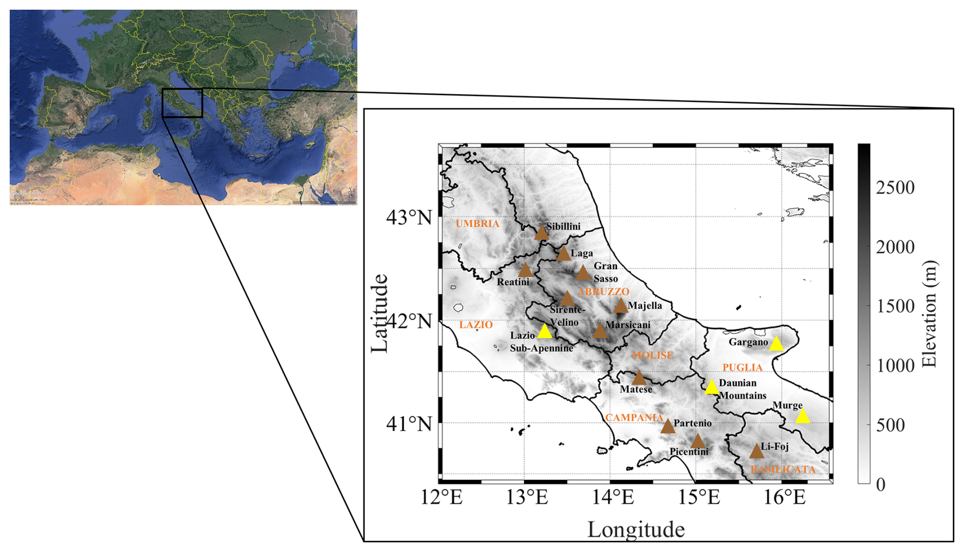
Figure 1 In the left panel is a map of the Mediterranean area, including the study region (highlighted as a solid-black-outlined box) is presented. The right panel shows a digital elevation model of the investigated area, with several mountain ranges mentioned in the main text. More specifically, the main Apennine reliefs are marked as filled-in brown triangles, whereas the filled-in yellow triangles indicate several Apennine offshoots. The black line shows the boundaries of the Italian administrative regions included in the study area (the official names of the regions are indicated in orange). Images credit: © Google Earth, Data SIO (Scripps Institution of Oceanography), NOAA, U.S. Navy, NGA (National Geospatial-Intelligence Agency), and GEBCO (General Bathymetric Chart of the Oceans).

2 Materials and methods

2.1 Study area

The Apennines Mountains consist of parallel mountain ranges extending for about 1200 km from northwest to southeast along the length of the Italian Peninsula. They are conventionally subdivided into three different sectors: the northern sector, including the Ligurian and the Tuscan–Emilian Apennines; the central sector, encompassing the Umbria–Marche Apennines and the Abruzzi Apennines; and the southern sector, comprising the Samnite and Campanian Apennines, the Lucan Apennines, and the Calabria and Sicily Apennines. In this study, we focused on a study region embracing a large portion of the central Apennines and a small sector of the southern ones (Fig. 1). This area extends from 40.5 to 43.5° N latitude and from 12.5 to 16.0° E longitude and includes the following Italian administrative regions: Umbria, Lazio, Abruzzo, Molise, Campania, Puglia (Apulia), and Basilicata. It has a very complex orography consisting of several mountain ranges. The main orographic features, highlighted by filled-in brown triangles in Fig. 1, are (from north to south) the Sibillini Mountains (2476 m a.s.l.), the Laga Mountains (2458 m a.s.l.), the Reatini Mountains (2217 m a.s.l.), the Gran Sasso area (2912 m a.s.l.), the Sirente–Velino mountains (2487 m a.s.l.), the Maiella massif (2793 m a.s.l.), the Marsicani Mountains (2285 m a.s.l.), the Matese massif (2050 m a.s.l.), the Partenio (1598 m a.s.l.), the Picentini mountains (1809 m a.s.l.), and the Vulture–Li Foj area (1365 m a.s.l.). Moreover, the study area also includes several Apennine offshoots, marked as filled-in yellow triangles in Fig. 1, such as the Lazio sub-Apennines (2063 m a.s.l.), the Daunian Mountains (1132 m a.s.l.), the Gargano massif (1065 m a.s.l.), and the Murge plateau (686 m a.s.l.). The study region is bounded by flat areas which gradually slope down to the Tyrrhenian Sea (to the west) and to the Adriatic Sea (to the east).

The climate of this area presents distinct Mediterranean features, with a precipitation maximum between late autumn and midwinter and a relevant minimum in midsummer. According to Crespi et al. (2018), the spatial distribution of the accumulated precipitation is strongly conditioned by the orography of the region and exhibits a marked west-to-east gradient, with drier conditions along the Adriatic sector. It is interesting to highlight that, on average, the highest annual precipitation amounts (up to 2200–2500 mm) are observed in the massifs of the southern Apennines, i.e. in the Matese, Partenio, and Picentini areas. Although they have a lower altitude than the mountains of the central Apennines, such reliefs lie in a relatively less complex orographic context, and therefore, they receive precipitation from a wide spectrum of synoptic patterns (Capozzi et al., 2022).

Regarding snow precipitation, the only climatological reference is the old study of Gazzolo and Pinna (1973). This work provided a coarse climatology for the HN, SCD, and NDS parameters for the whole Italian Peninsula, using the data collected by NHMS during the 1921–1960 period. According to Gazzolo and Pinna (1973), the major peaks of the central Apennines (Gran Sasso, Sibillini, and Laga mountains and Maiella) received, in the considered time interval, up to 400 cm of fresh snow per year. In the mountainous areas of the southern sector (Matese, Partenio, and Picentini), the average total yearly HN is slightly above 200 cm. In contrast to what is generally observed for the total precipitation, the snowfall amounts observed in the eastern slopes of the central Apennines and in the adjacent flat and coastal areas are higher than those measured in the western sectors. This can be related to the effects of the cold continental air masses coming from the Balkan region and eastern Europe, which stimulate abundant snowfall precipitation through two main mechanisms, namely the vertical transport of moisture and heat connected to their passage over the Adriatic Sea and the orographic forcing, which is related to their interaction with the mountain ranges. Regarding the SCD, the yearly climatological value is between 50 and 100 d (or greater) in the main reliefs of the central Apennines, whereas it is generally below 50 d in the southern massifs. The frequency of occurrence of snowfall events is very high (25–50 d) in the central sector, while, according to Gazzolo and Pinna (1973), it is lower than 20 d in the southern areas.

The mean annual temperature exhibits a strong altitudinal gradient, decreasing from 16-17 °C at the coastal areas and 13-14 °C at the base of the Apennines to, finally, 2-4 °C at the highest peaks of the central sector (Curci et al., 2021). As perfectly testified by the climatology presented in Brunetti et al. (2014), the valleys and the sub-mountain areas of the Abruzzo region have a mean annual temperature lower than the most of hilly regions of Campania, Puglia, and Molise. This difference is mainly due to the minimum temperature (Curci et al., 2021) and can be ascribed to the frequent occurrence, in the Abruzzo valleys, of the thermal inversion phenomenon.

2.2 Data rescue

In this study, we have exploited the database of the following four NHMS compartments: Naples, Bari, Rome, and Pescara. The data collected by the stations belonging to the NHMS network were published in the Hydrological Yearbooks, which are freely accessible in a printed version (i.e. as scanned images in portable document format) through the Italian Institute for Environmental Protection and Research (ISPRA) website (http://www.bio.isprambiente.it/annalipdf/, last access: 9 January 2024). The editing and publishing of the Hydrological Yearbooks were handled by the Departmental Office of the NHMS responsible for a specific compartment. Each Hydrological Yearbook contains the data collected in a certain year and is generally structured in two different parts. Part I includes the thermometric and pluviometric measurements, and the Part II contains a wide spectrum of data related to precipitation, hydrology, groundwater levels, exceptional events, and tide measurements (https://www.isprambiente.gov.it/en/projects/inland-waters-and-marine-waters/hydrological-yearbooks, last access: 9 January 2024). The snow data are included in Part II of the Hydrological Yearbooks from 1917 to 1934 and in Part I from 1935 onwards.

More specifically, the snow data are reported for the October to May period and consist of the following parameters: SCD, NDS, HS, and HN. From 1917 to 1934, the available measurements include the daily HN, the corresponding snow water equivalent amount, the monthly NDS value, and the HS value before the occurrence of a determined snowfall event. Subsequently, the snow data are reported in a different format. Regarding the SCD and NDS parameters, monthly data are available from 1935 to 1999 for the Naples and Rome compartments, from 1935 to 2000 for the Bari compartment, and from 1935 to 2013 for the Pescara compartment. The temporal coverage of HS data resembles the one of SCD and NDS; however, it should be highlighted that for this parameter only, three daily observations per month (at the end of each decade) are available from 1935 to 1971 and only one (in the last day of a determined month) in the subsequent periods. Concerning the HN variable, unfortunately, no data are available from 1935 to 1970, whereas monthly observations are reported from 1971. The snow measurements have been manually performed using a traditional nivometer consisting of a snowboard and a graduated yardstick (De Bellis et al., 2010). It is important to highlight that according to the NHMS standard, the monitored snow parameters are defined as follows:

• SCD is the total number of days in a given month or in a given season with snow depth on the ground ≥1 cm.

• NDS is the total number of days in a given month or in a given season on which the accumulated snowfall (i.e. the amount of fresh snow with respect to the previous observations) is at least 1 cm.

• HN is the daily or monthly amount of fresh snow (expressed in cm). The monthly value is intended as the sum of daily HN data observed in a determined month.

• HS is the daily snow depth on the ground (expressed in cm).

From 1917 to the end of the 1940s, the data availability is limited and is strongly conditioned by the period of the First and Second World Wars (in which many stations temporarily interrupted their monitoring activity). The number of stations reporting snow data increased in the early 1950s, and it was fairly stable until the end of the 1990s, except for some isolated drops (in 1989 and 1997). Subsequently, after the closure of NHMS, the data availability strongly decreased and was restricted to some stations of the Abruzzo region, which continued to collect snow data under the management of local regional authorities, and to the Montevergine Observatory station (southern Apennines), which autonomously continued the meteorological parameter recording (Capozzi et al., 2020).

In this study, we decided to consider the 1951–2001 period, which corresponds to the years with the highest number of data points. More specifically, we have digitised the SCD, NDS, HN, and HS data collected by stations having an elevation greater than 250 m a.s.l. In other words, we have excluded the stations located in flat areas or along the coasts, where the occurrence of snow is relatively rare. Using this criterion, we have retrieved 281 stations with elevations ranging between 288 and 2125 m a.s.l. Note that for the digitisation process, we have used a simple “key entry” method. Despite the recent introduction of new approaches and methodologies based on optical character recognition software and machine learning tools, manual transcription is still the most accurate technique for climate data digitisation. As shown by Brönnimann et al. (2006), the manual method has a lower error rate and fits the recommendations and the standards practises of the World Meteorological Organization well (World Meteorological Organization, 2016), although it is slower in terms of the amount of rescued data per unit of time. The digital templates have been developed in Microsoft Excel and have been structured into different spreadsheets, with one dedicated to the station metadata and the other one to the data of the available snow parameters.

A complete list of all rescued stations, with details about geographical coordinates (latitude, longitude, and height a.s.l.), the NHMS compartment to which a determined station belongs, and the percentage of available data, is provided in the Supplement (Table S1).

2.3 Data, quality control, and homogenisation

In this work, we have analysed the SCD and NDS data collected in the 1951–2001 period and the HN data measured between 1971 and 2001. We have decided not to consider the HS data as these have been reported in the Hydrological Yearbooks with a format consisting of three or one daily observations per month, which is not suitable for a reliable climatological analysis.

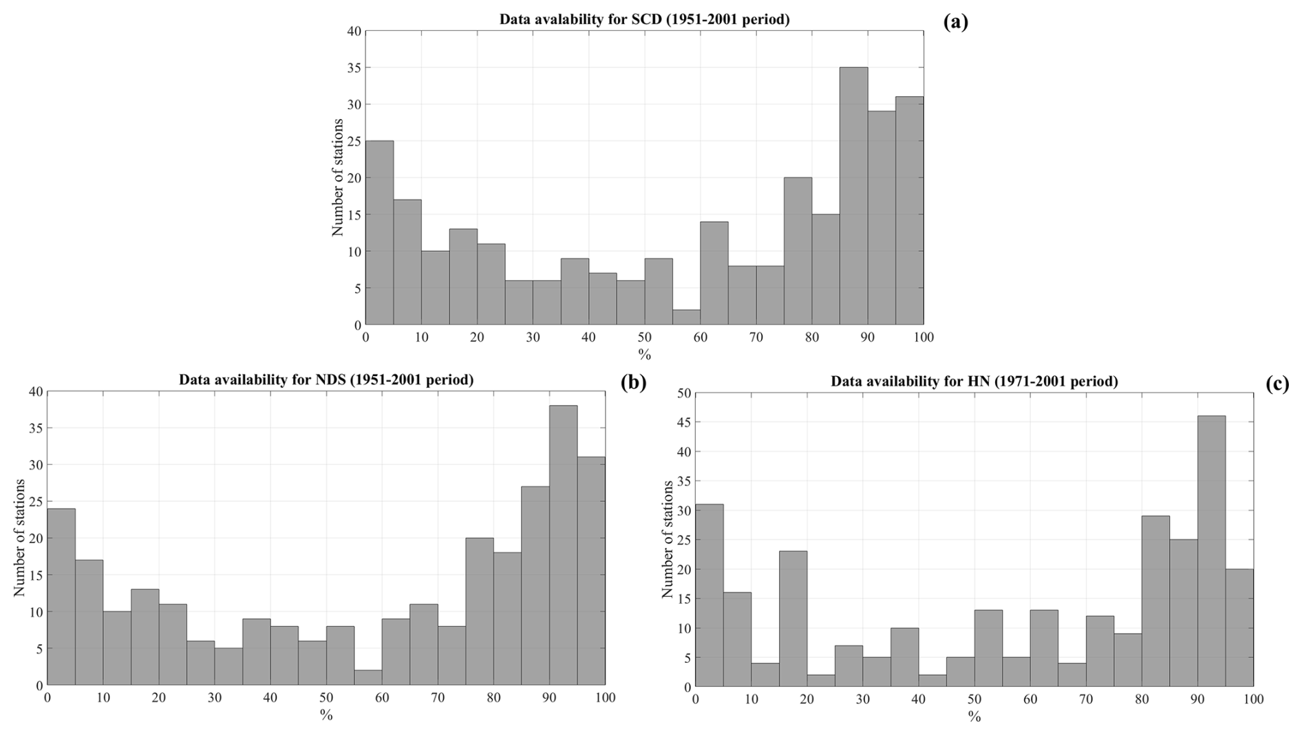
Figure 2 Histogram of the data availability (in %) for the considered snowfall parameters. SCD (a), NDS (b), and HN (c). Note that in this figure all rescued stations have been considered.

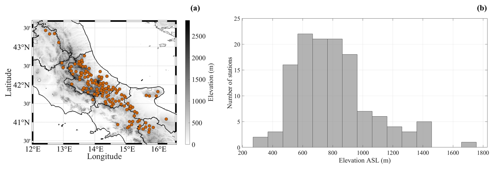
Figure 3 Panel (a) shows the location of the stations (129 in total) considered for the analyses carried out in this work. The black line shows the boundaries of the Italian administrative regions included in the study area. Panel (b) shows the number of available stations per elevation.

Figure 2 presents the histograms of the data availability for three considered parameters, namely SCD (Fig. 2a), NDS (Fig. 2b), and HN (Fig. 2c). The data availability has a clear bimodal distribution, with two distinct peaks, namely one between 0 % and 10 % and the other between 85 % and 100 %. From a simple visual inspection of Fig. 2, it emerges that a non-negligible fraction of the rescued stations has limited data availability. For SCD and NDS (HN), 39 % (37 %) of the measuring stations have a data availability of less than 50 %. According to the criteria suggested by the World Meteorological Organization (World Meteorological Organization, 2008), we have discarded the stations with less than 80 % of the available data in the observation period. Moreover, we have rejected some stations belonging to the Rome compartment, namely Abeto, Castelluccio di Norcia, Monte Terminillo (only for SCD and NDS), and Bagnara (only for SCD), due to the presence of many suspicious records. This screening yielded a subset consisting of 129 stations for which the positions are shown in Fig. 3a. The spatial distribution of the stations is quite uniform over the entire region, except for the northern side (Umbria–Marche Apennines); for this area, there are only four stations located at an altitude ranging between 529 and 750 m a.s.l. The density of the stations is particularly high in the proximity of the main mountain ridges of Abruzzi and Samnite Apennines. In the southern sectors, only one station (Montevergine Observatory) is located above 1000 m a.s.l. Regarding the elevation distribution, which is shown in Fig. 3b, a relevant number of stations (69) is between 600 and 900 m a.s.l., 27 stations are below 600 m a.s.l., and the remaining (33) are above 900 m a.s.l.; the elevation ranges from a minimum of 288 m to a maximum of 1750 m a.s.l.

The considered dataset has been subjected to an accurate quality control (hereafter QC). It is widely known, in fact, that the quality assurance of climate data is crucial to improve confidence in any further analysis. As pointed out in many papers, the reliability and the consistency of a historical climatological time series can be affected by several artefacts and errors and caused by instrument failures, human mistakes in data collection, and inaccuracies in the digitisation of paper-based data. In this study, we have developed a QC strategy consisting of three statistical tests:

• the gross error test, which flags the data that are above or below acceptable physical limits;

• the consistency test, which involves an inter-variable check; and

• the tolerance test, which is focused on outlier detection.

Note that this QC strategy has been applied to the monthly SCD and NDS time series available in the 1951–2001 period and to the monthly HN time series available in the 1971–2001 time segment.

The gross error test aims to identify the clearly erroneous values and consists of comparing the monthly SCD, NDS, and HN values to their physical limits. For SCD, we have checked for cases in which, for a determined month and for a certain station, the number of days with snow on the ground is greater than the number of days in that month (e.g. SCD is 32 d in January). For NDS, we have applied a very similar criterion, flagging the circumstances in which the NDS value is equal to or greater than the number of days in a determined month as “gross errors”. According to this criterion, the instance in which a new snowfall event occurred on every day of a certain month is considered an implausible situation. For monthly HN values, we have considered the limit (500 cm) recommended by World Meteorological Organization (2008).

The second step of the QC process aims to detect inconsistencies between the pairs of the investigated variables. More specifically, the purpose of this test is to detect the following instances: (i) the NDS value for a determined month and a certain station is greater than the SCD value; (ii) the NDS value for a determined month and a certain station is zero, and the HN value is greater than zero; (iii) the NDS value for a certain month and a determined station is greater than zero, and the NH value is null. By applying the gross test and the consistency checks, 1527 monthly invalid data points were found; in particular, 2.0 % of the erroneous data emerged from the gross test, whereas the remaining 98.0 % represent the outcome of the consistency test. A relevant fraction of the bad data can be attributed to instances in which the NDS value is greater than the SCD value. In some Hydrological Yearbooks, in fact, the NDS value is reported in the column dedicated to the SCD value, and vice versa. Therefore, in most of the cases, the identified errors have been easily corrected; in other circumstances, they have been discarded and replaced with a missing data marker.

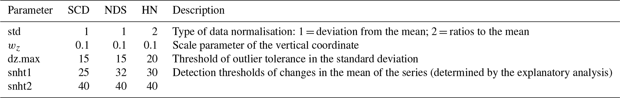
The tolerance test has been performed using the Climatol method. The latter has been developed by Guijarro (2018) and is widely employed for the QC, homogenisation, and filling the missing data for a set of climatological time series. The Climatol data processing starts with a normalisation of the original data. In this respect, Climatol offers different approaches for normalisation, depending on the climatological variable. In this study, the type of normalisation (std) has been set to 1 (which means that data normalisation is based on deviations from the mean) for SCD and NDS, whereas we selected std = 2 (which means normalising using the ratio to normal climatological value) for HN. The approach used by Climatol to detect outliers is inspired by the principles of the spatial consistency check. In particular, for any candidate time series, this method uses data from neighbouring stations to estimate a corresponding reference series as a weighted average, employing a geographic proximity criterion using Euclidean distances. In the default settings of the toolbox, the vertical and horizontal distances (expressed in metres and kilometres, respectively) between a suitable neighbouring station and the candidate one have the same weight. Following Buchmann et al. (2022) and taking into consideration the influence of altitude on the snow, in this study we have adjusted the scale parameter of the vertical coordinate (w_z) so that the elevation counts 100 times more; in other words, the approach used in our work means that an altitude difference of 500 m corresponds to a horizontal distance of 50 km. The estimated reference series are used to create a time series of anomalies for their corresponding observed series by subtracting the estimated values from the observed ones. The values of the anomaly time series that exceed a determined threshold (dz.max) are labelled as outliers, and so the correspondent data in the original series are discarded. More specifically, the dz.max value, set by default to ±5 standard deviations, was properly tuned to ensure that the flagged outlying values were not rejected because of their extremeness. After several sensitivity experiments in which we manually inspected the data flagged as potential outliers, the dz.max parameter has been set as follows: dz.max = 15 for SCD and NDS, and dz.max = 20 for HN. Using this criterion, the tolerance test flagged as outliers only two NDS monthly observations related to the Frigento and Roccasicura time series.

Climatol has been employed in this study to also check the homogeneity of the investigated time series. The use of this toolbox for the homogenisation of snow data has been explored, with encouraging results, in some recent works (Buchmann et al., 2022, 2023). As described in detail by Guijarro (2018) and by Kuya et al. (2022), the Climatol homogenisation method is based on the standard normal homogeneity test (SNHT; Alexandersson, 1986) for the identification of the breaks and on a linear regression approach for the adjustments (Easterling and Peterson, 1995). The SNHT falls within homogenisation procedures that are able to identify an inhomogeneity without knowing a priori the time of the break point in the time series and that can also estimate the magnitude of the detected break. The basic idea underlying this method consists of using neighbouring stations as a reference to identify the inhomogeneities in the station being tested (the candidate station). Such an assumption requires the existence of a sufficient correlation level between the test and reference stations. More specifically, SNHT uses a normalised series of the ratios/differences (hereafter Q) between, e.g., precipitation/temperature at the candidate station and the neighbouring reference stations. The test is based on the null hypothesis that the Q series has a constant mean level, i.e. that the candidate series is homogeneous, and the alternative hypothesis that the mean level of the Q series changes abruptly from one level to another at some time. For each point of the time series, a test value, based on a comparison between the means of the two subsamples before and after the potential breakpoint, is computed as described in detail in Alexandersson and Moberg (1997). The null hypothesis is rejected if the maximum test value of all dividing points in the Q series is greater than a predefined critical level. In Climatol, the SNHT is applied to the anomaly time series previously introduced in the description of the tolerance test. In brief, the Climatol homogenisation process is structured in two procedures, namely the application of the SNHT on stepped overlapping temporal windows and on the whole series. In the first one, called “stepped overlapping windows”, the toolbox computes the SNHT test for all series, retaining the maximum SNHT value for each series. The series having a maximum SNHT value greater than a specific threshold (snht1) are split into two subseries at the point of the maximum SNHT value. Subsequently, the sub-series are tested again, and the procedure is iterated until the maximum SNHT value of the sub-series is below the snht1 threshold. After this procedure, the test is applied to the whole series in order to detect further breaks, using a threshold value snht2. Once a break for a determined candidate time series is detected, the latter is corrected back in time, starting from the most recent homogeneous time interval. The break magnitude corrections are computed as the variation in the mean before and after the homogenisation procedure. More specifically, given a time series Y, the correction factor (CF) is calculated as follows:

$$\begin{array}{}\text{(1)}& \text{CF}={\displaystyle \frac{{\mathit{\sigma }}_Q{Y}_{\mathrm{b}}+Q_{\mathrm{m}}}{{\mathit{\sigma }}_Q{Y}_{\mathrm{a}}+Q_{\mathrm{m}}}},\end{array}$$

where Y_b and Y_a are the mean values between the beginning of the measurements of Y and the break point (before) and from the break point to the end (after), respectively. Q is the non-standardised ratio time series, defined as the ratio between the reference and candidate, and σ_Q and Q_m are the standard deviation and mean of Q, respectively. Additional details about the calculation of the adjustment factor can be found in Guijarro (2018), Kuya et al. (2022), and Buchmann et al. (2023). The last step of Climatol processing consists of the filling of all missing values using the weighted ratios of neighbouring series and in the production of the final high-quality homogeneous and complete time series. It is important to highlight that Climatol offers the opportunity to carry out a first explanatory analysis of the data, which is very useful for the tuning of several parameters, including snht1 and snht2. The main settings adopted to run Climatol for tolerance test of QC and homogenisation are listed in Table 1.

Table 1 Main settings used to run Climatol (Guijarro, 2018) for quality control and homogenisation of the investigated SCD, NDS, and HN time series.

Using this set-up, Climatol flagged seven SCD and two NDS time series as inhomogeneous. Details about the dates on which the breaks occurred and the corresponding value of SNHT are supplied in the Supplement (Table S2). From a visual inspection of such a time series, the results of the homogeneity test seemed very reasonable. The identified breaks were further examined against the metadata reported on the Hydrological Yearbooks. However, the latter contain only some useful information that allowed us to verify only if the stations were relocated (this is not the case for any of the stations identified as inhomogeneous). We therefore do not have enough information to determine the cause of the inhomogeneities. We decided to adopt a precautionary approach and, therefore, the detected breaks were accepted.

2.4 Cluster analysis

In order to build up a reference climatology for the three parameters investigated in this study, the SCD, NDS, and HN time series have been grouped into different clusters, each representing a specific climatic zone. Following the previous literature, we used a multivariate method based on the principal component analysis (PCA) and cluster analysis (CA). This approach has been employed in different areas (Kidson, 1994; Sumner et al., 1995; Fragoso and Tildes Gomes, 2008; Capozzi et al., 2023), proving to be reliable in the classification of meteorological data.

To search for dominant spatial patterns, the (non-rotated) PCA has been applied in T mode to a dataset consisting of n “observations” (i.e. the stations; 110 for SCD, 114 for NDS, and 120 for HN) and m “variables” (i.e. the monthly data; 612 for SCD and NDS and 372 for HN). It is important to highlight that the PCA has been employed not as a merely data reduction technique but as a method which guarantees that only the fundamental modes of variation in the data are taken into account. Using the scree plot, we have determined the appropriate number of principal components (PCs) for each of the three investigated parameters. After this pre-processing, the well-known non-hierarchical k-means method (Anderberg, 1973) was then performed using the selected PC scores as input. In the selection of the optimal number of clusters, we searched for the best trade-off between subjective evaluation, based on the patterns expected from the climatic and topographic drivers, and the semi-objective metrics (“elbow method”).

2.5 Statistical analyses

In order to evaluate the magnitude of the trend slope in SCD and NDS time series, the well-known Theil–Sen non-parametric test was employed (Sen, 1968). This procedure is largely used in the hydro-meteorological framework because of its robustness in the presence of outliers in the series (Song et al., 2015; Bartolomeu et al., 2016; Ortiz-Gómez et al., 2020). To assess the trend magnitude, the Theil–Sen procedure estimates the trend slope in a determined sample for all data pairs. The median of all samples computed for each data pair coincides with the steepness of the trend. On the other hand, the statistical significance was assessed with the Mann–Kendall non-parametric test (Mann, 1945; Kendall, 1962). This test is a rank-based method for assessing the presence of increasing or decreasing monotonic trends in time series data, and it is often used because of its property of requiring minimal assumptions about the data that need to be tested (Hamed, 2008). The significance levels of 0.05 and 0.1 (i.e. the 95 % and 90 % confidence levels, respectively) have been used to test the null hypothesis that there is no trend in the data. It is important to highlight that prior to the application of these statistical tests, the pre-whitening technique was used to reduce the effect of lag-one autocorrelation in the analysed time series (e.g. Caloiero et al., 2011; Tramblay et al., 2013).

In addition, to measure the relationship between the linear trend of the analysed parameters and the elevation, we employed the traditional Pearson correlation coefficient (hereafter ρ).

2.6 Wavelet analysis

The wavelet analysis is a very appealing alternative to the classic short-time Fourier transform for the geophysical time series analysis and periodicities examination. The Wavelet tool, in fact, allows discriminating not only the main frequencies in a non-stationary series but also localising them in time (Percival, 2008). This is a very useful feature for the analysis of climate data, whose variability is typically modulated by nonstationary processes. Because of such remarkable advantages, we have decided to apply the wavelet transform (WT) to the clustered–averaged SCD and NDS time series involved in this study to identify their oscillation in the frequency domain. Among the main WT categories (Grinsted et al., 2004), we have chosen the continuous wavelet transform (CWT), which is particularly suitable for the analysis of scale- and time-dependent features of a time series. The CWT searches for a similarity between the investigated signals and a well-known mathematical function (the wavelet). The latter is applied several times with different scales to the considered time series and at different temporal locations. Similar to other studies (e.g. Carey et al., 2013; Marcolini et al., 2017b), we have decided to apply the Morlet function as the Wavelet function. Additional details about the mathematical formulation of this function, as well as about the wavelet analysis, and the methods used to assess the statistical significance of the power spectrum can be found in Grinsted et al. (2004). It is important to highlight that the CWT presents some deficiencies at the edges of the investigated time series. Therefore, it is useful to introduce a cone of influence, where the results are uncertain (Torrence and Compo, 1998). The CWTs of two signals can be combined to obtain the cross-wavelet transform (XWT), which offers the possibility of detecting the areas, in the time–frequency domain, where the two CWTs share common features in terms of power and relative phase (for mathematical details, see Grinsted et al., 2004).

3 Results

3.1 Regionalisation

The PCA of monthly SCD, NDS, and HN time series allowed the extraction of the essential modes of spatial variability. A detailed description of the principal component analysis (PCA) results for each of the three investigated variables is offered in Appendix A. According to the evidence provided by the scree plot, we have considered the first four PCs for SCD (which account for 73 % of the total variance), the first nine PCs for the NDS (which explain 70 % of the total variance), and the first four for the HN (which account for 70 % of the total variance). Such levels of explained variance seem to be acceptable, given the considerable number of stations and the complex nature of the snow variables. It is interesting to highlight that, in all three cases, the first PC explains most of the variance (61.2 % for SCD, 51.8 % for HN, and 47.7 % for NDS). From the analysis of PC scores, which can be regarded as standardised spatial patterns, it clearly emerges that the first PC reflects the altitude-related variability in the three snow indicators across the whole elevation range (see Figs. A2, A4, and A7 in Appendix A). The other considered PCs explain a very limited portion of variance (generally ranging between 1 and 8 %) and might be linked with several factors, such as the difference between the eastern and western sides of the Apennines, the distance from the sea, and the hours of direct sunlight, as well as with local patterns strongly conditioned by the orography.

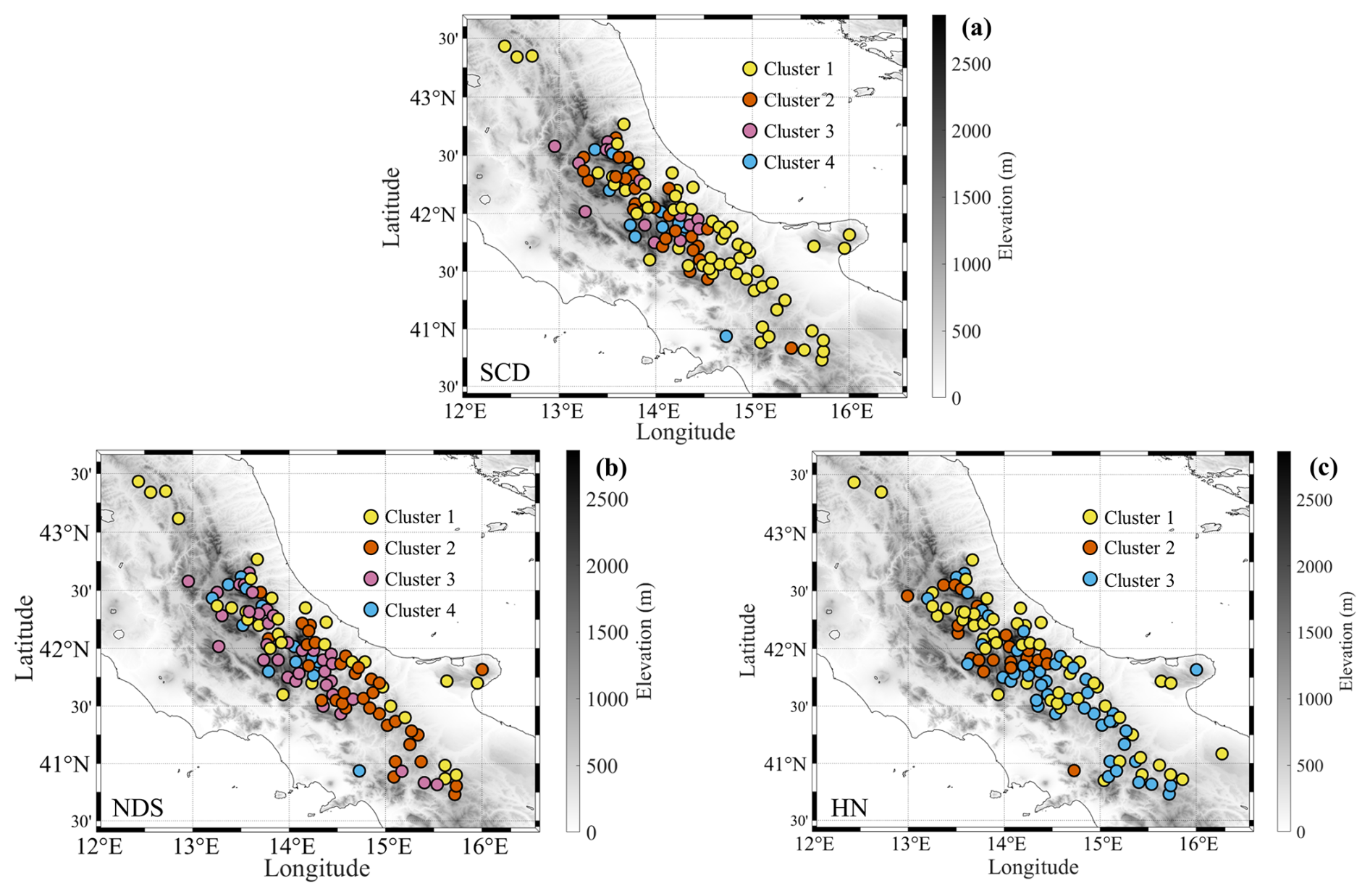
Figure 4 Clustering of stations based on monthly data of SCD (a), NDS (b), and HN (c). The stations are colour-coded according to the cluster memberships.

The PCA scores from the selected PCs were employed as input for the k-means algorithm. After several tests and sensitivity analyses to assess the cluster reproducibility and stability, four clusters were chosen for SCD and NDS and three for HN. The clustering of the available stations based on monthly SCD, NDS, and HN data are presented in Fig. 4. From a visual inspection of this figure, as well as of Table 2, it is straightforward to notice that the clusters are relatively well separated in altitude. Starting from SCD (Fig. 4a), the identified groups are populated by a number of stations that is inversely proportional to the median elevation. More specifically, as revealed by Table 2, cluster 1 comprises 58 stations and has a median altitude of 648 m a.s.l. (min–max: 288–910 m a.s.l.), cluster 2 counts 26 stations with a median elevation of 815 m a.s.l. (min–max: 550–954 m a.s.l.), and cluster 3 includes 14 stations and has a median elevation of 1000 m a.s.l. (min–max: 750–1157 m a.s.l.). Finally, cluster 4 includes 12 stations with an altitude greater than or equal to 1000 m a.s.l. (median value: 1290 m a.s.l.). The altitudinal range of the stations is around 400 m for all clusters, except cluster 1. The latter, in fact, includes not only low-elevation sites but also stations located on the eastern and southern mountain slopes of the central Apennines chain, which are located in topographic contexts unfavourable to the persistence of snow on the ground due to the high number of hours of direct sunlight.

Table 2 For each of the investigated snow indicators (SCD, NDS, and HN), the number of stations belonging to a determined cluster and the stations' median and range elevation (minimum–maximum) are shown.

The four groups that emerged from the clustering of NDS data are shown in Fig. 4b. According to Table 2, most of the stations are nearly equally distributed among the first three clusters (31 belong to cluster 1, 34 to cluster 2, and 35 to cluster 3). Cluster 1 includes low-elevation sites (median altitude 569 m a.s.l.; min–max: 288–850 m a.s.l.) and stations located in the main valleys of Abruzzo region. The second cluster has a slightly higher median elevation (700 m a.s.l.; min–max: 520–910 m a.s.l.) and brings together a relevant number of hilly sites of the southern and Samnite Apennines, as well as several stations located on the eastern side of Maiella mountains. The stations belonging to the third cluster span a significant altitudinal range (from 650 to 1375 m a.s.l.) and have a median elevation of 879 m a.s.l. The fourth cluster is very similar to the SCD cluster 4; it includes, in fact, only high-elevation sites having a median elevation of 1220 m a.s.l. (min–max: 1000–1430 m a.s.l.).

The clustering of HN data yielded three regions (Fig. 4c); the first one (cluster 1) includes 52 stations with a median elevation of 603 m a.s.l. (min–max: 288–948 m a.s.l.). The second one (cluster 2) comprises 45 sites with a median altitude of 829 m a.s.l. (min–max: 625–1137 m a.s.l.), whereas cluster 3 includes 23 sites, all located in the central Apennines (except one, Montevergine Observatory, which is situated in the southern sector), with a median elevation of 1210 m a.s.l. (min–max: 800–1750 m a.s.l.). This classification is clearly conditioned not only by altitude but also by local climatic and topographic factors, which may generate large differences in the snowfall amount among stations located at similar altitudes. Most of the stations belonging to cluster 4 are located in the proximity of the Maiella and Marsicani mountains, where the orographic forcing and low-level wind convergence lines are able to strongly enhance the snow precipitation.

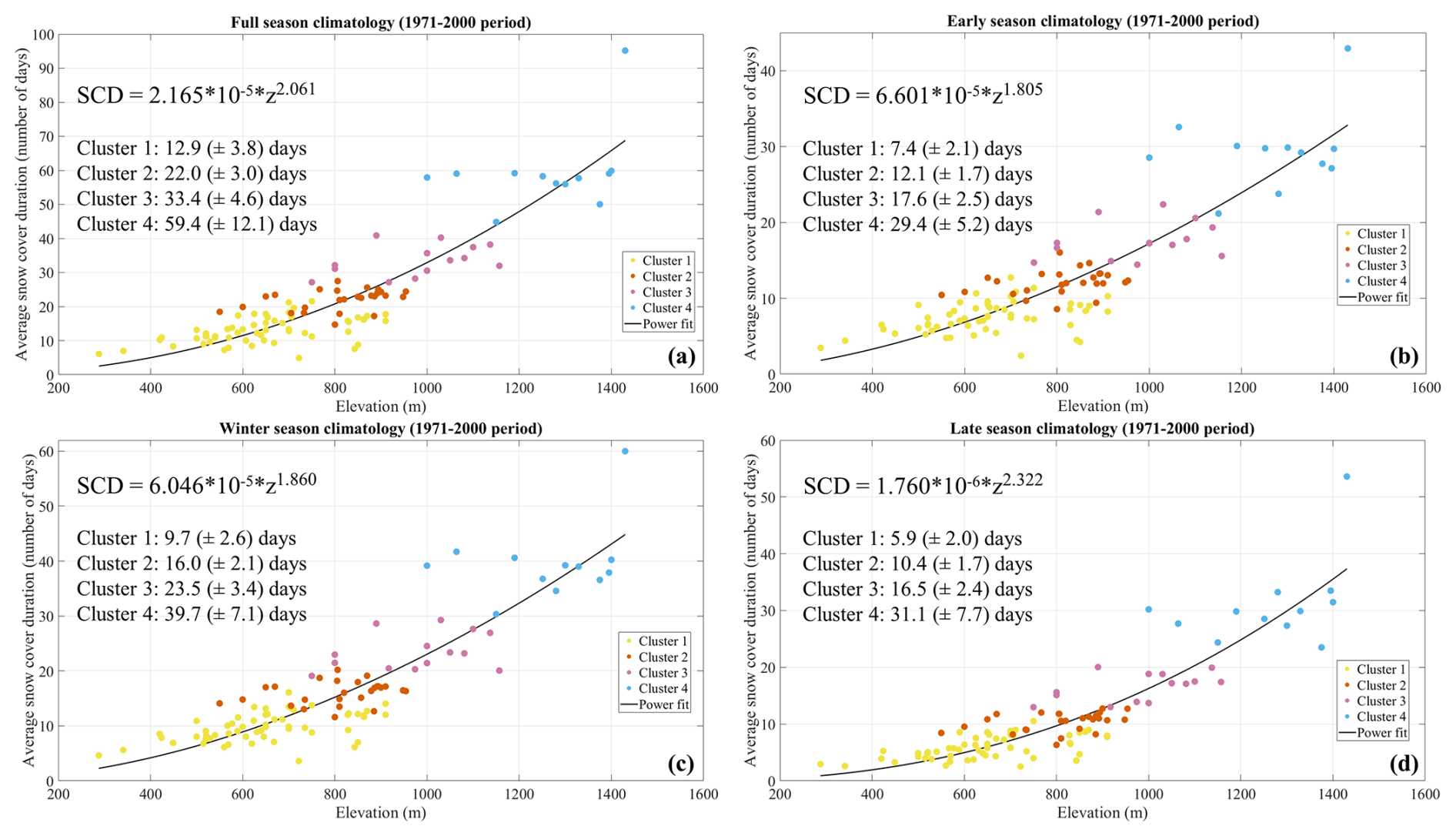
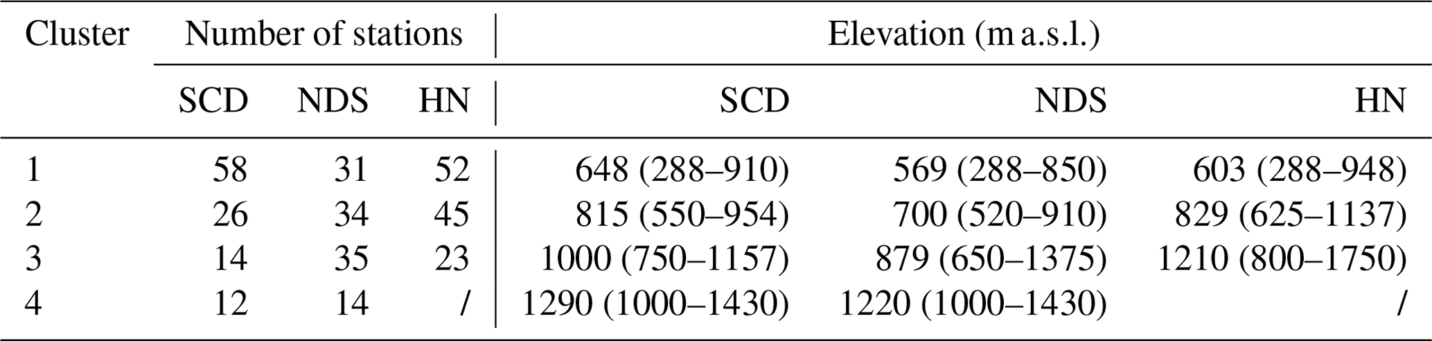
Figure 5 Climatology of snow cover duration (SCD) for (a) full, (b) early, (c) winter, and (d) late seasons. Average values are for the period 1971–2000. Each point represents a station that is colour-coded according to the membership cluster. The solid black line represents the power fit. The text boxes show the power fit equation and the average and standard deviation values for each cluster.

3.2 Climatology for the 1971–2000 period

Starting from the clustering results, we have built up reference climatology for different snow seasons, namely early season (from November to January), winter season (from December to February), late season (from February to April), and full season (from November to April). This seasonal partition is similar to that generally adopted in previous studies (e.g. Matiu et al., 2021), with some small adjustments, depending on the climatic features of the study area and on the elevation range of the available stations. Figure 5 presents the climatology 1971–2000 for the SCD parameter. More specifically, for each of the four seasons previously introduced, the altitudinal distribution of the average SCD (expressed in a number of days) is shown. Each point represents one station and is colour-coded according to the membership cluster (note that we follow the same colour-coding adopted in Fig. 4). In addition, on each panel, the cluster-averaged values and the associated spatial standard deviation are also reported. As expected, there is a clear altitudinal gradient that grows as the elevation increases. In the full season, the SCD average rises by ≈9 d from cluster 1 (which presents a climatological value of 12.9 (±3.8) d) to cluster 2 (22.0 (±3.0) d) and by ≈11 d from cluster 2 to cluster 3 (33.4 (±4.6) d), whereas the difference among cluster 3 and cluster 4 (59.4 (±12.1) d) is steeper (it is 26 d). The relationship between the average SCD and elevation is efficiently modelled by a power fit, as testified by the coefficient of determination (R²), which ranges between 0.72 (early season) and 0.78 (late season). Note that the power curve function obtained for a determined season is shown on the corresponding panel as a solid black line, assuming that the average snow cover duration is the dependent variable (SCD) and the elevation the independent one (z). It is interesting to highlight that the differences among clusters reduce in the early season, whereas they are larger in the winter season. In addition, it is worth noting that in cluster 4 the distribution becomes more dispersed, as testified by the standard deviation values. The spatial distribution of the average seasonal SCD over the study area is shown in Fig. B1 in Appendix B. In all seasons, the highest-average SCD value has been found in Camposto (1430 m a.s.l.), which is located on a plateau east of the Laga Mountains. In this site, the local topographic conditions are particularly favourable to the persistence of the snow on the ground.

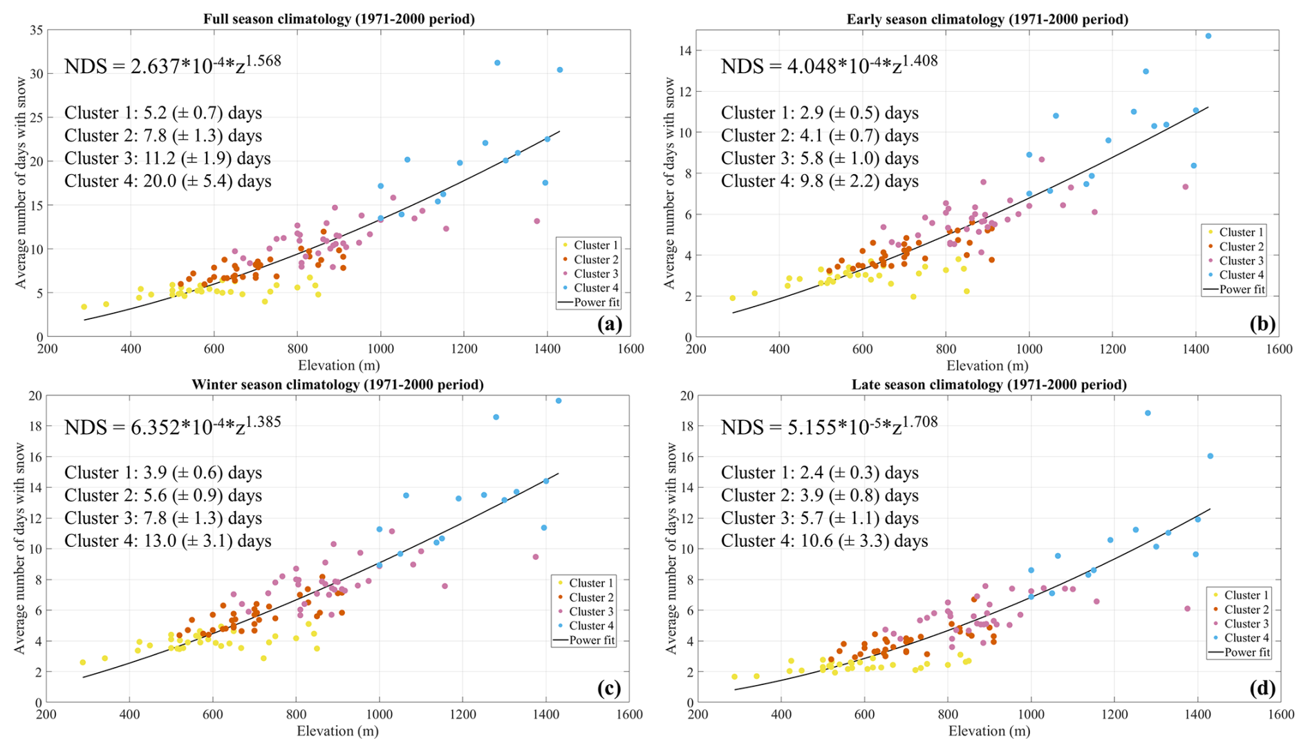
Figure 6 Climatology of the number of days with snowfall (NDS) for (a) full, (b) early, (c) winter, and (d) late seasons. Average values are for the period 1971–2000. Each point represents a station that is colour-coded according to the membership cluster. The solid black line represents the power fit. The text boxes show the power fit equation and the average and standard deviation values for each cluster.

The climatology for NDS is presented in Fig. 6. The average NDS values found for the available stations spread over the considered altitudinal range and follow, also in this case, a distribution well captured by a power law function (R²=0.78 for all seasons). This behaviour suggests the existence of an altitudinal gradient, which, similar to what has been discovered for SCD, rises with increasing elevation. The cluster-averaged climatological NDS values (shown for each season on the corresponding panel) provide confirmation in this regard; in the full season, the average NDS is 5.2 (±0.7) d for cluster 1, 7.8 (±1.3) d for cluster 2, 11.2 (±1.9) d for cluster 3, and 20.0 (±5.4) d for cluster 4. Above 800 m a.s.l., there is a clear increase in the spatial variability, which maximises within cluster 4 in all seasons. The difference between clusters does not exhibit a relevant seasonal dependence, although in winter a slight increment of the gap in average NDS value between clusters 1 and 2 and between clusters 3 and 4 has been detected. It is worth pointing out that, in the full and late seasons, the highest climatological NDS value has been observed in the southern Apennines (Fig. B2), more precisely in Montevergine Observatory (1280 m a.s.l.). This result is only apparently surprising. As briefly discussed in Sect. 2.1, the southern Apennines massifs included in the investigated area are well exposed to different air masses (i.e. to both continental air masses coming from Balkan regions and to maritime air masses coming from the Atlantic), so they receive larger precipitation amounts than the central sectors. According to the results of our study, this aspect also reflects on the frequency of occurrence of snowfall events, which, on the Partenio massif, is larger than many mountainous sites of the central Apennines located at the same altitude or slightly above, as demonstrated by Fig. B2.

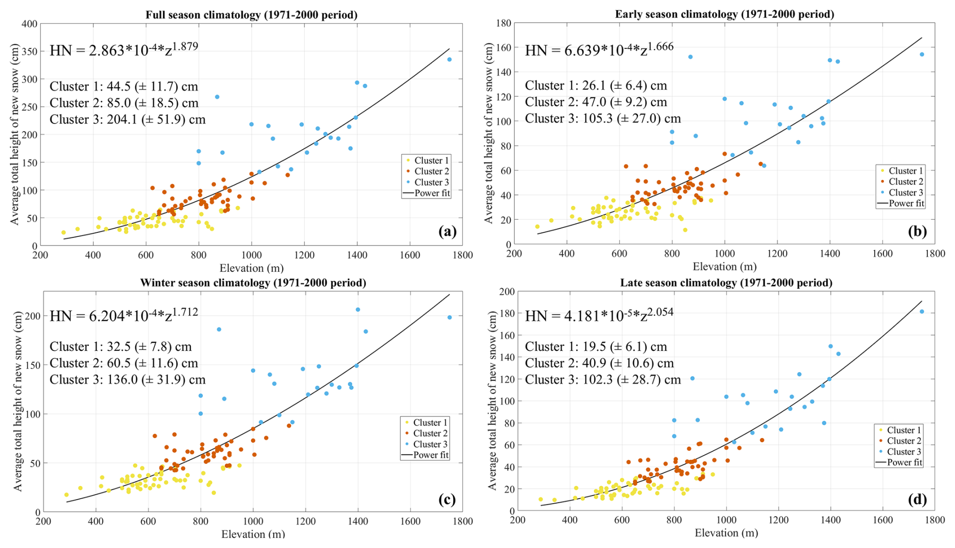
Figure 7 Climatology of the height of new snow (HN) for (a) full, (b) early, (c) winter, and (d) late season. Average values are for the period 1971–2000. Each point represents a station that is colour-coded according to the membership cluster. The solid black line represents the power fit. The text boxes show the power fit equation and the average and standard deviation values for each cluster.

The HN climatology is presented in Fig. 7. As for SCD and NDS, the analysed region exhibits a pronounced variability, mainly driven by the elevation, with a minimum, in the full season, of 24 cm in Lanciano (288 m a.s.l.) and a maximum of 335 cm in Monte Terminillo station (1750 m a.s.l.) in the Reatini Mountains. According to the scatter diagrams of Fig. 7, there is a clear separation between the three groups identified by the cluster analysis. In the full season, the climatological HN value is 44.5 (±11.7) cm for cluster 1, 85.0 (±18.5) cm for cluster 2, and 204.1 (±51.9) cm for cluster 3. The latter shows a remarkable variability, which is related not only to the altitude but also to the incidence of orographic effects. In this respect, in the Abruzzo region, there are several stations below 1000 m a.s.l. that received, in the considered reference period, relevant snowfall amounts that are comparable to sites belonging to higher altitudinal bands. This is the case for Nerito (800 m a.s.l.), in which the full-season climatological HN value is 148 cm; Rosello (890 m a.s.l.), in which the average HN value is 167 cm; and Sant'Eufemia a Maiella (870 m a.s.l.), the most impressive case, for which the average HN value is 268 cm (Fig. B3). In the late and winter seasons, the snowfall amounts increase by ≈80 % from cluster 1 to cluster 2 and by ≈124 % from cluster 2 to cluster 3. In the late season, we have detected a steeper altitudinal gradient instead. Cluster 2 receives, on average, more than twice (+109.7 %) the total HN value observed for cluster 1, whereas in cluster 3 the snowfall amounts grow by 150 % with respect to cluster 2.

3.3 Trend analysis

The linear trend analysis has been applied to both individual SCD and NDS time series, as well as to cluster-averaged time series. The latter have been obtained, for each of the investigated seasons, as the arithmetic mean of the values of stations belonging to a determined cluster.

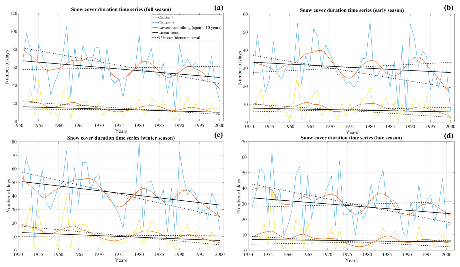
Figure 8 Cluster 1 (yellow line) and cluster 4 (blue line) snow cover duration (SCD) time series for full (a), early (b), winter (c), and late (d) seasons. The solid black line shows the linear trend and the dashed black line the 95 % confidence interval for linear trend, whereas the vermilion line marks the loess smoothing (span = 10 years). The period from 1951 to 2001 has been considered.

Starting from SCD, Fig. 8 shows the cluster 1 (solid yellow line) and cluster 4 (solid blue line) time series for the 1951–2001 period. Note that we decided not to plot the behaviour over time for clusters 2 and 3 for ease of presentation. According to Sect. 3.1, cluster 1 and cluster 4 include stations belonging to different altitudinal bands (the median elevation is 648 and 1290 m a.s.l., respectively), and, therefore, they reflect two well-separated nivometric regimes. From a simple visual inspection of this figure, it clearly emerges that the investigated signals exhibit a negative tendency (see the solid black line). More specifically, the trend magnitude (expressed in number of days per 10 years) is more pronounced in the full season (−3.4 [−7.3 to 1.7] d per 10 years for cluster 4 and −1.1 [−2.6 to 0.2] d per 10 years for cluster 1) and in the winter season (−3.2 [−6.0 to 0.0] d per 10 years for cluster 4 and −1.1 [−2.5 to 0.2] d per 10 years for cluster 1). Note that the values indicated in square brackets indicate the 95 % confidence interval for linear trend. In the other seasons (early and late), cluster 1 shows a negligible trend, whereas for cluster 4 a decreasing rate of −1.1 [−3.3 to 1.0] d per 10 years and −1.8 [−4.5 to 0.6] d per 10 years has been detected, respectively. As revealed by Table 3, the trends are statistically significant only in the full and winter seasons. More specifically, in the winter season a negative tendency significant at 90 % confidence level has been found for clusters 1, 2, and 4, whereas for cluster 3 the linear trend is significant at the 95 % confidence level. In the full season, robust tendencies have been discovered only for clusters 1 and 4. According to Table 3, in all seasons the trend magnitude gradually increases from cluster 1 to cluster 4; so, in other words, it rises with increasing altitude, especially in the full and winter seasons. In addition, Table 3 shows, for each cluster, the percentage of positive, negative, and no trends (i.e. the subset of tendencies ranging between −0.4 and 0.4 d per 10 years), and the portion of trends significant at 95 % confidence level. As can be expected, most of the stations exhibit a negative tendency. In particular, for clusters 2, 3, and 4, the percentage of negative trends is above 60 % in all seasons and is greater than 90 % for clusters 3 and 4 in winter and for cluster 4 in the full season. For cluster 1, there is a clear prevalence of negative trends only in the full and winter periods, whereas in early and late seasons most of the stations belonging to such cluster present a negligible trend. Moreover, the fraction of significant and negative tendencies has an altitudinal dependency that is more linear and evident in full and winter seasons. In the latter season, half of the stations pertaining to clusters 3 and 4 exhibit a negative trend significant at 95 % confidence level. Another distinguishable behaviour of the signals shown in Fig. 8 is the strong interannual variability, which is particularly pronounced in cluster 4. This is a distinct feature of the precipitation records collected in mid-latitudes that, with regard to the Apennine area, has been just emphasised in previous works (e.g. Capozzi et al., 2022). Focusing on the full season, in cluster 4, the highest SCD values have been observed in the 1962/63 (105.3 d), 1952/53 (98.2 d), and 1980/81 (95.8 d) seasons, whereas the lowest SCD values have been observed in the 1989/90 (10.6 d), 2000/01 (22.0 d), and 1963/64 (26.0 d) seasons. The season in 1962/63 was also notable in terms of SCD for cluster 1 (43.0 d), although the highest value for this group was observed in 1955/56 (45.6 d), which was one of the coldest and snowiest seasons of the 20th century (e.g. D'Errico et al., 2022). In cluster 1, the lowest values have been recorded in the 1989/90 (0.9 d), 1960/61 (2.6 d), and in 1963/64 seasons (2.7 d). Superimposed to the decreasing trend, the Apennine's SCD also shows considerable decadal variations that are well captured by the 10-year locally weighted scatterplot smoothing (loess). The latter, marked as a vermilion line in Fig. 8, is a robust non-parametric regression technique proposed by Cleveland (1979). By inspecting the behaviour of loess fit, it is possible to detect four periods characterised by an extensive duration of snow cover, namely the early 1950s, the 1960–1970 period, the late 1970s–early 1980s, and the early 1990s, and four time segments with reduced SCD, namely the late 1950s, the mid-1970s, the late 1980s, and the late 1990s. The decadal oscillation of SCD seems to be a common feature of all considered seasons and is more relevant in cluster 4 time series.

Table 3 For each cluster (CL) and for each season (full (F), early (E), winter (W), and late (L)), the average SCD trend value (expressed as a number of days per 10 years), the percentage of positive and negative trends, and the percentage of no trends are presented. For positive and negative trends, the fraction of significant tendencies is also indicated. Note that no trends are defined as tendencies ranging between −0.4 and 0.4 d per 10 years. The statistical significance of the trends is coded as follows: ** for 95 % and * for 90 %.

Table 4 For each cluster (CL) and for each season (full (F), early (E), winter (W), and late (L)), the average NDS trend value (expressed as a number of days per 10 years), the percentage of positive and negative trends, and the percentage of no trends are presented. For positive and negative trends, the fraction of significant tendencies is also indicated. Note that no trends are defined as tendencies ranging between −0.4 and 0.4 d per 10 years. The statistical significance of the trends is coded as follows: ** for 95 % and * for 90 %.

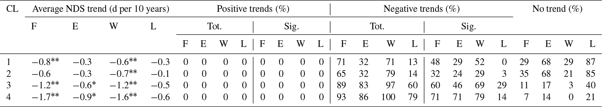
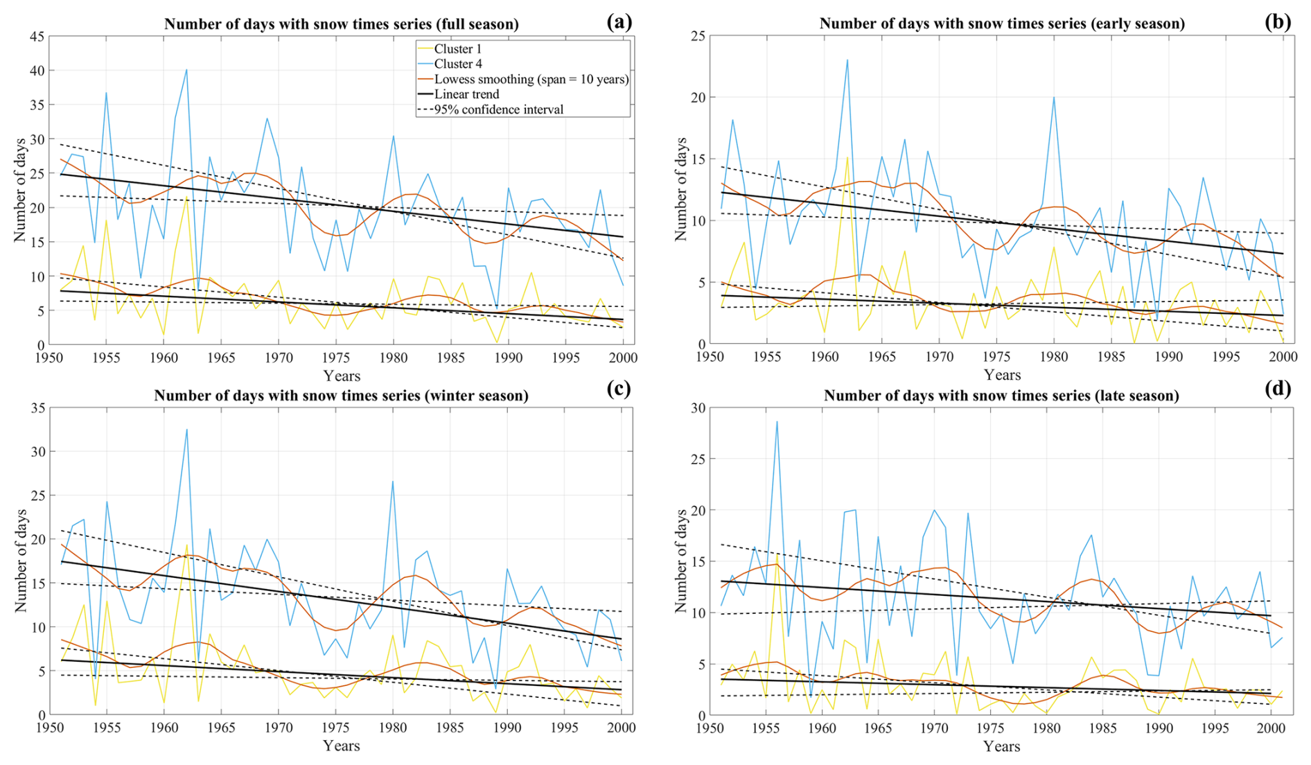
Figure 9 Cluster 1 (yellow line) and cluster 4 (blue line) indicate the number of days with snowfall (NDS) time series for the full (a), early (b), winter (c) and late (d) seasons. The solid black line shows the linear trend, and the dashed black line the 95 % confidence interval for linear trend, whereas the vermilion line marks the loess smoothing (span = 10 years). The period from 1951 to 2001 has been considered.

The NDS time series exhibit behaviour very similar to that described for SCD, as demonstrated by Fig. 9. For clusters 1 and 4, we have detected a gradual decrease in the frequency of occurrence of snowfall events, again particularly pronounced in full and winter seasons. In the former, the linear trend analysis revealed a negative tendency of −1.7 [−3.0 to −0.5] d per 10 years for cluster 4 and of −0.8 [−1.3 to −0.1] d per 10 years for cluster 1, whereas in the latter the tendency magnitude is −1.6 [−2.5 to −0.6] d per 10 years for cluster 4 and −0.6 [−1.2 to −0.1] d per 10 years for cluster 1. Such trends are statistically significant at the 95 % confidence level, as indicated by Table 4. Strong negative tendencies have been also found, in the full and winter seasons, for the other cluster-averaged time series (except for cluster 2, whose trend is not statistically significant in the full season). As for SCD, in the late season, cluster-averaged trends are negligible and range between −0.1 [−0.7 to 0.4] d per 10 years (cluster 2) and −0.6 [−1.6 to 0.2] d per 10 years (cluster 4). In the early season, negative trends significant at the 90 % confidence level have been detected for clusters 3 and 4 (trend magnitude is −0.6 [−1.2 to −0.1] d per 10 years and −0.9 [−1.6 to −0.3] d per 10 years, respectively). Table 4 shows that long-term tendencies taking a direction towards NDS reduction are prevalent in all seasons for clusters 3 and 4, with the percentage up to 97 %–100 % in the winter season, whereas this result is not valid for clusters 1 and 2, in which the no trend fraction predominates in the early and late seasons. The percentage of stations having a trend significant at the 95 % confidence level found for clusters 3 and 4, as well as the trend magnitude, is substantially larger than that discovered for clusters 1 and 2. Such results suggest the existence of a relationship between the long-term tendency and elevation in terms of statistical significance and magnitude. The decadal trend that emerged from the analysis of the SCD time series is also evident in NDS signals, as highlighted by the loess fit in Fig. 9. Similar to what has been observed for SCD, this decadal behaviour is more pronounced in cluster 4. The NDS signals also exhibited very strong interannual variability, especially in the 1950–1960s. In cluster 4, the frequency of occurrence of snowfall was particularly higher in the 1962/63 (40.1 d), 1955/56 (36.8 d), and 1969/70 (33.0 d) full seasons. It is interesting to highlight that the second and the third snow seasons more lacking in snow events occurred in the 1950–1960s during the seasons of 1963/64 (7.7 d) and 1958/59 (9.7 d). The lowest NDS value has been detected in the 1989/90 season (5.1 d). The latter has been the weakest season in terms of snowfall occurrence also for cluster 1 (0.3 d). Very low values (1.6 and 1.4 d, respectively) have also been observed in 1963/64 and 1960/61, respectively. Moreover, the 1962/63 (21.5 d), 1955/56 (18.1 d), and 1953/54 (14.5 d) seasons were the three richest seasons in terms of snow episodes for cluster 1.

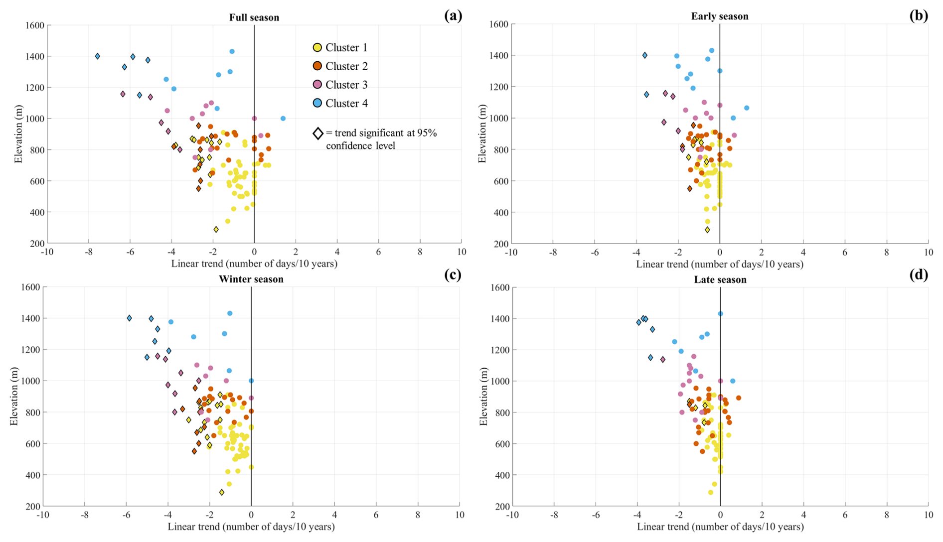
Figure 10 Seasonal snow cover duration (SCD) trends (expressed as a number of days per 10 years) as a function of elevation for the full (a), early (b), winter (c), and late (d) seasons. Each point represents one station and is colour-coded according to the membership cluster. Trends significant at 95 % confidence level are displayed as diamond markers.

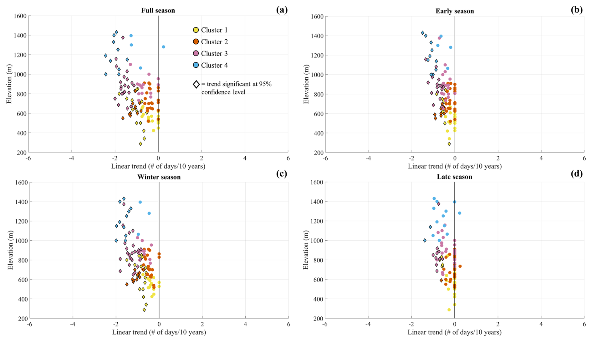
Figure 11 Seasonal number of days with snowfall (NDS) trends (expressed as a number of days per 10 years) as a function of elevation for full (a), early (b), winter (c), and late (d) seasons. Each point represents one station and is colour-coded according to the membership cluster. Trends significant at 95 % confidence level are displayed as diamond markers.

Linear trends for individual stations as a function of elevation at seasonal timescales are shown in Fig. 10 (SCD) and in Fig. 11 (NDS). Such diagrams provide more compelling evidence about the relationship between the trend magnitude and altitude. As a general result, a moderate correlation between the two variables has been found for both snow indicators. More specifically, for SCD, the correlation is stronger in the late and winter seasons ($\mathit{\rho }=\left|\mathrm{0.63}\right|$ and $\left|\mathrm{0.62}\right|$, respectively), whereas it is slightly weaker in the late season ($\mathit{\rho }=\left|\mathrm{0.43}\right|$). For NDS, different results emerged in terms of seasonal variability in the correlation. The latter maximises in the early season ($\mathit{\rho }=\left|\mathrm{0.59}\right|$), whereas it is lower in the late season ($\mathit{\rho }=\left|\mathrm{0.46}\right|$). A visual comparison between Figs. 10 and 11 also reveals that SCD trends are characterised by a larger variability than NDS, especially at altitudes greater than 1000 m a.s.l. It is worth noting that in the full season the maximum negative trend (−7.6 [−11.8 to −2.4] d per 10 years) was found for Capracotta (1400 m a.s.l.), a station belonging to cluster 4. The maximum positive tendency (1.4 [−3.7 to 6.0] d per 10 years) has been detected for Pietracamela (1000 m a.s.l.), a station that is part of the same cluster. This result synthesises the strong variability and uncertainty that affects the linear trend estimation at high-elevation ranges well, which can be interpreted as a consequence of the strong year-by-year fluctuations, as well as of the local orographic effect incidence.

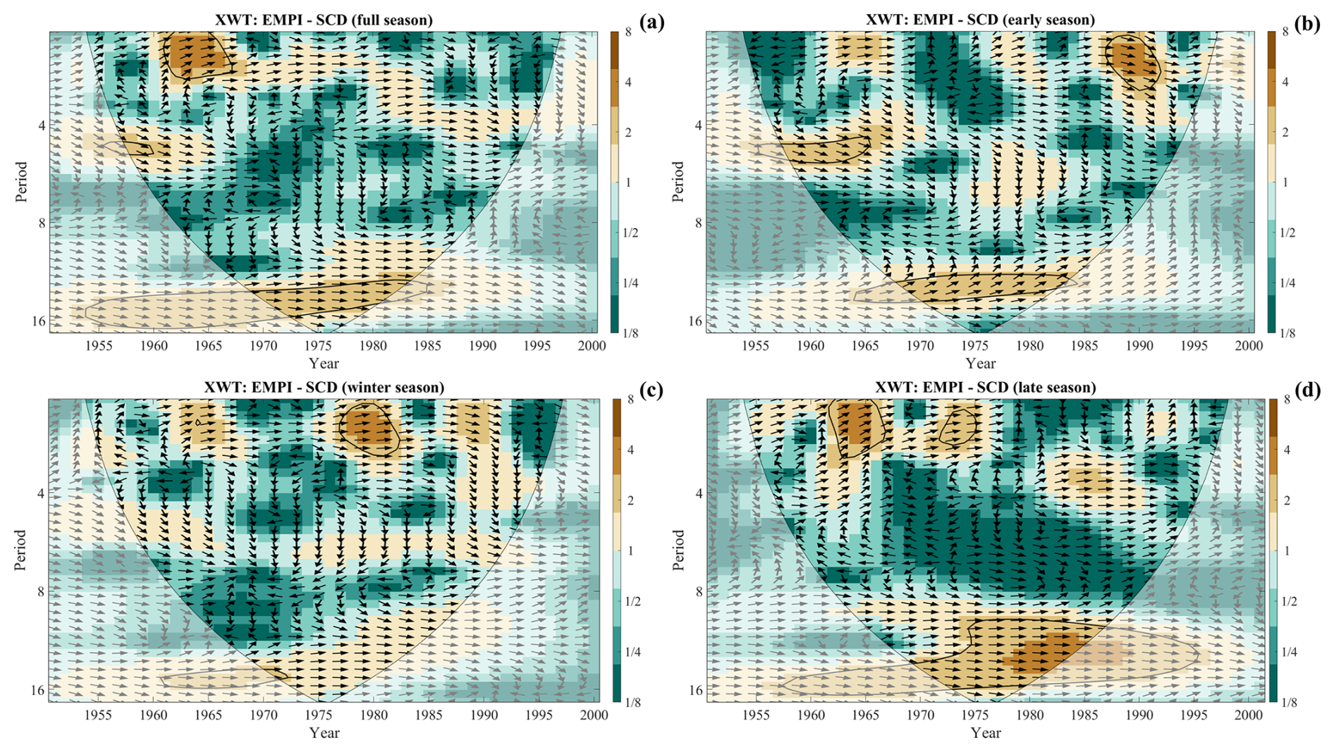
Figure 12 Cross-wavelet transform (XWT) between Eastern Mediterranean teleconnection Pattern Index (EMPI) and the cluster 4 snow cover duration (SCD) time series for the (a) full season, (b) early season, (c) winter season, and (d) late season. The black arrows indicate the phase relationship between the respective time series. The thick contour designates the 5 % significance level against red noise; the cone of influence, where edge effects might distort the picture, is shown with a lighter shade. All XWT spectra refer to the period 1951–2001. Note that black arrows pointing to the right indicate that the signals are in phase.

3.4 Connections with large-scale atmospheric patterns: preliminary evaluations

A natural evolution of our study is a further investigation aimed at identifying the main drivers controlling the SCD and NDS variability in the considered Apennines region. Recently, several research activities (e.g. Hammond et al., 2018; Annella et al., 2023; Bertoldi et al., 2023) dealt with this topic, taking into account both “local” variables, such as temperature and precipitation, and “global” drivers such as the large circulation patterns. According to the general results achieved for the Alpine region, the role of temperature and precipitation in controlling the snow presence is strongly modulated by the elevation. Generally, at low elevations, most of the snow variability is explained by temperature, whereas at high elevations the precipitation has a greater relative importance (e.g. Bertoldi et al., 2023). However, in a very recent study that documented the exceptional snow drought conditions that affected the Italian Alps during the winter season in 2021/22, Colombo et al. (2023) discovered an increasingly relevant role of warming air temperature in driving the snow drought events in the whole investigated elevation range (864–2200 m a.s.l.). For the Apennines, Annella et al. (2023) found that the reduction in SCD observed in the Montevergine Observatory could be mainly attributed to the increasing trend in temperature, which was statistically significant in winter and late seasons in the considered time interval (1931–2008). In light of such results, it may be speculated that the decline in SCD and NDS discovered in our study has been mainly driven by the rising temperature tendency that occurred in the second half of the 20th century. Currently, we are not able to demonstrate this assumption with a deep investigation. Most of the historical temperature and precipitation records collected in the study area, in fact, are not accessible in a ready-to-use digitised format. Therefore, a complete attribution analysis is left for future analysis. However, here we discuss some preliminary linkages between the decadal trend observed in our study for SCD and NDS signals and the large-scale circulation patterns. More specifically, our analysis starts from the results of Annella et al. (2023). From this study, it emerged that short-time and decadal fluctuations in SCD in Montevergine Observatory are strongly modulated by two teleconnections patterns, namely the Arctic Oscillation (AO) and the Eastern Mediterranean teleconnection Pattern (EMP). The first one is a fundamental mode of the Northern Hemisphere climate variability as it describes simultaneous shifts in several features of the polar vortex (air temperature, air pressure, and the location and strength of the jet stream). The EMP has been introduced by Hatzaki et al. (2007) and is referred to as the difference in the 500 hPa geopotential height anomaly between the eastern Atlantic and the eastern Mediterranean. Using the Wavelet tool, we searched for the relationship between these two large-scale patterns and SCD and NDS signals. Note that the corresponding index for AO (the AO index; hereafter AOI) has been retrieved from the Climate Prediction Centre of NOAA's National Weather Service (Climate Prediction Center, 2024), whereas the EMP index (hereafter EMPI) was reconstructed in Capozzi et al. (2022), using version 3 of the NOAA-CIRES 20th Century Reanalysis dataset (Allan et al., 2011), following the method described in Hatzaki et al. (2009). The XWT between the AOI and SCD cluster-averaged time series did not reveal noticeable results, except for the winter season in which a significant common power area on a 2-year band was detected between 1960 and 1965. In this region of the time–frequency spectrum, the AOI and SCD are in an anti-phase relationship. More interesting evidence came from the analysis of the relationship between EMP and SCD. Figure 12 presents the XWT between the EMPI and SCD cluster 4 time series for all four considered seasons. We have chosen the cluster 4 SCD time series as a reference for this analysis because its behaviour in the time–frequency spectrum can be regarded as highly representative of the one observed for the other three clusters. This aspect has been confirmed by the CWT, which depicts a coherent picture among the clusters that is characterised by a significant peak in the ≈12–14 year band from 1960s to 1990s and by two high-frequency (≈2 years) oscillations, namely one located between 1951 and 1955 and the other one between 1960 and 1965. The only exception is cluster 1 in which the decadal oscillations are not statistically relevant. Starting from the full season (Fig. 12a), it is easy to detect a significant common power in the ≈12–16 year band from 1955 to 1985 and between 1960 and 1965 in the ≈0–2 year band. A close connection between EMPI and SCD can be also found in the ≈12–14 year band in the early season (Fig. 12b) from 1965 to 1985, whereas in winter (Fig. 12c), the common power area on a decadal scale is restricted between the early 1960s and early 1970s and falls entirely within the cone of influence. A very strong and significant connection between the investigated signals has been found in the late season (Fig. 12d) on the ≈12–16 year band. The common power area, in this case, extends from the late 1950s to the mid-1990s, so it embraces almost the entire analysed period. Some linkages in the high-frequency region have been detected between 1955 and 1965 (≈5 year), in 1985–1990 (≈0–2 year band) in the early season, between the late 1970s and early 1980s (≈0–2 year band) in the winter season, and, finally, in the 1960–1965 and in the early 1970s (≈0–2 year in both cases) in the late season. The right-pointing black arrows in the significant power areas indicate that EMPI and SCD clearly swing in phase on a decadal timescale, adding further evidence about the close time–frequency connection among the signals. The XWT between EMPI and NDS cluster 4 time series draws a similar picture, as testified by Fig. 13. In this case, there is a close and significant connection on a decadal scale only in the full season (Fig. 13a) and in the late season (Fig. 13d). The common power areas are localised in the same spectrum regions mentioned for SCD. In the ≈0–2 year band, relevant connections between EMPI and NDS have been found in the 1961–1965 period in all seasons, between the late 1970s and early 1980s in winter (Fig. 13c), and in the early 1970s in the late season. In the early season (Fig. 13b), a common power area also appears in the ≈5 year band between the mid-1950s and mid-1960s. The two signals are generally in a close in-phase relationship, except for some significant areas in the high-frequency region where there is a slight lag between the two signals.

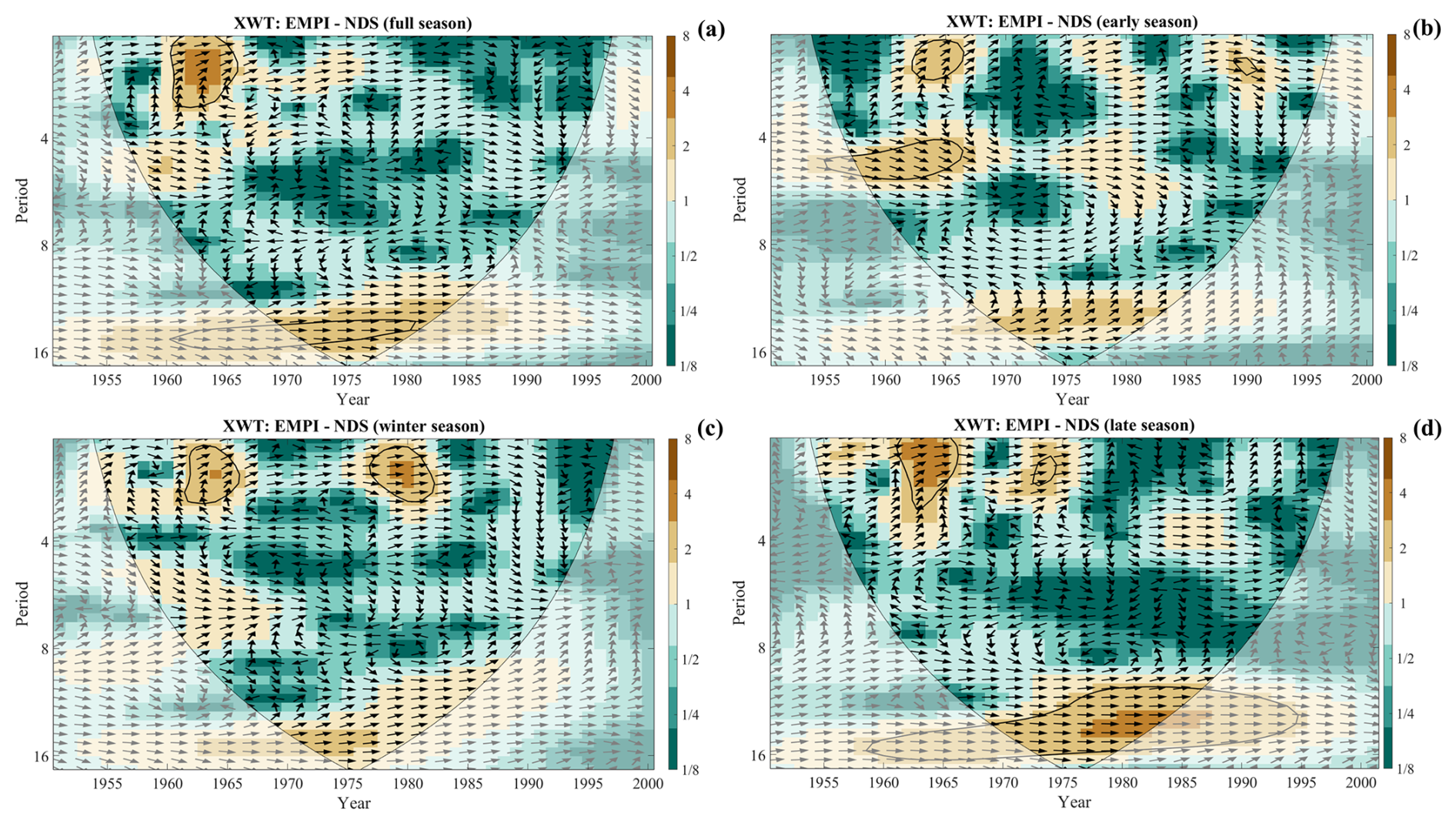
Figure 13 Cross-wavelet transform (XWT) between the Eastern Mediterranean teleconnection Pattern Index (EMPI) and the cluster 4 number of days with snowfall (NDS) time series for the (a) full season, (b) early season, (c) winter season, and (d) late season. The black arrows indicate the phase relationship between the respective time series. The thick contour designates the 5 % significance level against red noise; the cone of influence, where edge effects might distort the picture, is shown with a lighter shade. All XWT spectra refer to the period 1951–2001. Note that black arrows pointing to the right indicate that the signals are in phase.

The direct in-phase connection existing between the investigated snow indicators and the EMPI is in line with what should be reasonably expected about the influence of EMP on snow variability in the central and southern Apennines. The positive phase of the EMP pattern, in fact, is associated with positive 500 hPa geopotential anomalies over the northern Atlantic and with negative ones over central and eastern Mediterranean basins (Hatzaki et al., 2007). This synoptic pattern generally drives Arctic or Polar cold continental air masses towards Italy and, therefore, is clearly favourable for snow occurrence and persistence on the ground in the Apennines, as previously demonstrated in Capozzi et al. (2022) and in Annella et al. (2023). The negative phase of EMP depicts a very different configuration, which generally brings mild weather conditions in the considered area.

4 Discussion

In this study, thanks to the rescue of a large amount of manual snow observations collected by NHMS during 1951–2001, it was possible to build up a new, updated and solid reference climatology for an area, the Apennine regions, in which the information about past nivometric regime are scarce and very fragmented. For all considered snow indicators and for all investigated seasons, we found a relevant altitudinal gradient that grows as the elevation increases. This result exhibited a seasonal dependence for SCD and HN. More specifically, in the first case, the altitudinal gradients are steeper in winter and reduce in the early season, whereas for HN the altitudinal gradient is more pronounced in the late season. The clusters including the stations above 1000 m a.s.l. showed a strong spatial variability that is mainly related to the orographic effects. In this respect, our results are in accordance with some previous works (e.g. Blanchet et al., 2009; Bertoldi et al., 2023) related to the Alpine region.

Our analysis has revealed that in the considered Apennine region the SCD and NDS parameters exhibited a similar behaviour in terms of long-term and decadal trends. For both variables, a decreasing tendency has been detected in the 1951–2001 period. The observed variations are strongly connected with the season (i.e. they are more relevant in winter) and show a marked dependence on the elevation. It is obviously not straightforward to contextualise such results in the available literature because the linear trend magnitude and their statistical significance are strongly dependent on the analysed time window. Focusing on papers that considered periods having a good overlap with the present work, it clearly emerges that our study confirms the local and general tendencies observed for SCD and NDS in the Mediterranean area. Regarding SCD, the declining tendency highlighted in this study is in agreement with the local trends found for Apennines (e.g. Petriccione and Bricca, 2019; Annella et al., 2023), as well as with the outcomes presented for several Alpine regions (e.g. Klein et al., 2016; Marcolini et al., 2017b; Marke et al., 2018; Matiu et al., 2021; Bertoldi et al., 2023). Another common point between our results and previous works lies in the elevation dependence of SCD trends. More specifically, this aspect has been discussed in Marcolini et al. (2017b), who analysed SCD and HS time series collected in the Adige catchment (northeast of Italy) from 1980 to 2009. They found a reduction in both variables at low- and high-altitude sites, although a difference emerged between the behaviour of stations located above and below 1650 m a.s.l. In sites located below this altitude threshold, the decline in SCD and HS was larger. This work concludes that areas under 1650 m a.s.l. are more sensitive to climate variability and to temperature increase than high-elevation regions. Matiu et al. (2021) have reported a similar and more generalised result for the Alpine region; they found a decreasing trend in SCD below 2000 m a.s.l., while no remarkable variations have been detected above 2000 m a.s.l., at least in the period from November to May. The elevation dependence of snow trends has been also highlighted in a very recent work (Bertoldi et al., 2023) focused on the northeastern Italian Alps. Although this study is focused on HN indicators, it reported evidence comparable, at least in part, to SCD-based studies. On a monthly basis, negative trends were found in the lowest-elevation range (0–1000 m a.s.l.), with some positive trends from January to March above 2000 m a.s.l., while the intermediate elevation band (1000–2000 m a.s.l.) showed a strong variability with no robust tendencies. Averaged seasonal trends are negative for all elevation ranges; instead, in absolute terms, the maximum negative trend was found at intermediate levels.

Unfortunately, the stations available in our study cover a restricted altitudinal band (the only station situated above 2000 m a.s.l., Campo Imperatore, has very limited data availability), so we are not able to reconstruct the behaviour of SCD and NDS trends over the elevation range considered in previous studies for Alps and to identify a critical altitudinal band that separates different regimes characterised by opposite trend direction. Overall, the results of our study show that low and intermediate Apennine levels (288–1430 m a.s.l.) are experiencing a decline in SCD that is similar to what is generally observed in the Alps. However, in our case, most of the significant trends have been found in the core of the snow season (i.e. in the winter), whereas in the Alps the percentage of negative trends was substantially higher in spring months (e.g. Matiu et al., 2021).

The NDS is a less-studied variable than other snow indicators such as SCD, HN, and HS. Our results confirm some evidence found in Switzerland by Marty (2008). From this study, in fact, a long-term downward tendency in snow days emerged for the 1948–2007 period. The decreasing NDS signal is stronger in the low-altitude zone, whereas the higher stations showed a marked variability. Terzago et al. (2010) also found a decrease in NDS for the Piedmont region (1971–2009 period). In a subsequent work, related to a more extended period (1926–2010), Terzago et al. (2013) discovered a decline in the fraction of precipitation falling as snow in the western Alps; in line with our study, the drop in snow events was found to be more relevant in winter season.

It is interesting to point out that the linkages between EMP and snow indicators described in Sect. 3.4 have not been reported in any previous work related to the Alpine region. For this area, most of the available studies searched for connections with other large-scale circulation patterns, such as the North Atlantic Oscillation (NAO), the AO and the Mediterranean Oscillation. The results are generally ambiguous and strongly dependent on the considered region and time interval (e.g. Durand et al., 2009; Kim et al., 2013; Marcolini et al., 2017b; Bertoldi et al., 2023). For the 1930–2020 period, Colombo et al. (2022) found that NAO, winter NAO, Atlantic Multidecadal Oscillation, and AO were anticorrelated with the standardised snow water equivalent index during different phases of the snow season.

Regarding the AO, from the preliminary results presented in this study based on the cross-wavelet transform, it emerged that it exerts a less relevant influence than EMP on the nivometric regime of the investigated Apennine region. However, we feel that additional analyses are necessary to better assess the relationships between this important atmospheric mode and the snow variability in the study area. Two previous studies dedicated to the Apennines (Capozzi et al., 2022; Annella et al., 2023) found that the recovery in some snow indicators observed after 2000 is closely linked to the AO trend. It is possible to assume that a non-negligible difference might exist between the western and eastern sectors of the Apennines (the first ones might be more “sensitive” to the AO variability).

As stated in Sect. 1, ground observations are crucial for the assessment of long-term snow variability and trends, especially in mountainous areas. However, it is necessary to bear in mind that manual snow measurements have several limitations, mainly related to the observer's errors in reading and recording the measurement and also poor siting (World Meteorological Organization, 2008). A possible source of uncertainty that affect the dataset rescued in this study, and consequently the results just discussed, is related to the incorrect counting of snow days in a determined month (i.e. NDS parameter). As an example, the observer might have considered a day to be snowy when snowfall occurred without leaving any trace on the ground. In addition, in many contexts, the HN measurements can be very uncertain due to the environmental conditions, such as turbulence and/or strong winds, which may generate snow drifts and spatial inhomogeneity in snow depth.

5 Conclusions

According to the Intergovernmental Panel on Climate Change (IPCC) report on a high mountain (Hock et al., 2019), a general decrease in snow cover duration, glaciers, and permafrost due to climate change has occurred over the last few decades. The strong loss in the mountain cryosphere is likely to have relevant repercussions for the global population that relies on the water stored in mountain snow and ice for their water supply. Despite the serious impacts of mountain cryosphere loss, for several reasons, many mountain areas remain under-researched. In the Mediterranean, an example in this sense is represented by the Apennine region.

A considerable lack, in fact, exists in the knowledge of the past snow variability for this area, although it has a good record of past in situ observations. This study has provided a contribution to bridge this gap through the rescue and analysis of the snow precipitation measures manually collected between 1951 and 2001 by the Italian National Hydrological and Mareographic Service in an area including a large part of the central and southern Apennines. After being subjected to QC and homogenisation procedures, the rescued dataset, consisting of monthly data on the snow cover duration (SCD), number of days with snow (NDS), and height of new snow (HN), has been primarily analysed to retrieve a reference climatology (1971–2000 period). To pursue this aim, using a methodology based on principal component analysis and k-means clustering, we have grouped the available stations in different clusters for each snow indicator. This classification has been mainly driven by the altitude and, second, by other factors controlling the spatial variability in snow precipitation, such as the distance from the sea, the site exposure, the hours of direct sunlight, and local orographic features. The presented snow climatology greatly enhances and expands the existing historical database of several key snow-related variables, SCD, NDS, and HN, for which continuous and high-quality measures are difficult to find. In addition, it constitutes an added value for research focused on the comprehension of climate dynamics in mountainous areas, as well as on future changes in snow precipitation in the Mediterranean region, and provides useful information for a wide range of application fields, concerning also the socio-economic impacts of snow precipitation.

Furthermore, using familiar statistical methodologies (the Sen's slope estimator and the Mann–Kendall test), we have identified the linear trend for SCD and NDS time series (the HN series have not been considered for this analysis due to the limited length of the available records). Both variables exhibited a negative tendency for the 1951–2001 period. We found that SCD and NDS trends are strongly dependent on altitude, in terms of magnitude and level of confidence. More specifically, the signal of a decrease in the length of snow cover on the ground and in the frequency of occurrence of snowfall gradually grows with altitude and is generally very strong for stations located above 1000 m a.s.l. Considering the entire snow season (i.e. the full season from November to April), SCD trends statistically significant at the 90 % confidence interval have been discovered for cluster 1 (−1.1 [−2.6 to 0.2] d per 10 years) and for cluster 4 (−3.4 [−7.3 to 1.7] d per 10 years). For NDS, trends significant at 95 % confidence interval have been detected for clusters 1, 3, and 4 (−0.8 [−1.3 to −0.1] d per 10 years, −1.2 [−2.2 to −0.2] d per 10 years, and −1.7 [−3.0 to −0.5] d per 10 years, respectively). At a seasonal scale, a larger fraction of negative and significant trends has been found in the winter season for both variables. In the early and late seasons, the aliquot of significant tendencies strongly reduces, especially in clusters 1 and 2. In addition, we found that SCD trends exhibit a more pronounced variability and uncertainty than NDS, especially in cluster 4 (which includes, for both snow indicators, only stations above 1000 m a.s.l.). In the considered Apennine area, the SCD and NDS variables also show fluctuations at a decadal scale, as well as a remarkable interannual variability, in accordance with the findings of previous studies (e.g. Annella et al., 2023). The decadal behaviour gradually emerges with increasing altitude and is particularly relevant in cluster 4.

Despite some uncertainties and sources of errors, which have been briefly discussed in the previous section, this study can be considered the first Apennine-wide assessment of snow climatology and long-term trends based on in situ observations. The information provided by this work contributes to the reconstruction of historical snow variability in the mountainous areas and paves the way for many future research activities. In this respect, future studies will be primarily devoted to deeply understanding the physical mechanisms that control the evolution over time of the investigated snow variables. Regarding this aspect, we provided some preliminary results by means of a wavelet analysis. More specifically, from the cross-wavelet transform of the Eastern Mediterranean teleconnection Pattern Index (EMPI) and cluster 4 SCD and NDS time series, a significant common power emerged in the ≈10–16 year band. The two signals are phase-locked, so we can conclude that on a decadal scale the SCD and NDS behaviour in the investigated Apennines area mirrors the evolution of EMP. Future analyses should be oriented to better assess the influence of other teleconnection patterns (in particular the Arctic Oscillation) on the observed interannual variability.

In addition, other efforts may be made to (i) extend the investigated period back and forward in order to further increase the robustness of the trend analysis and to contextualise the observed SCD and NDS tendencies in a broader time horizon and (ii) to replicate this study for the northern Apennine sector and for the rest of the southern Apennine through the rescue of nivometric stations belonging to the remaining Italian National Hydrographic and Mareographic Service compartments.

Appendix A

In this Appendix, we provide a detailed description of the principal component analysis (PCA) results for each of the three investigated variables: snow cover duration (SCD), number of days with snowfall (NDS), and height of new snow (HN).

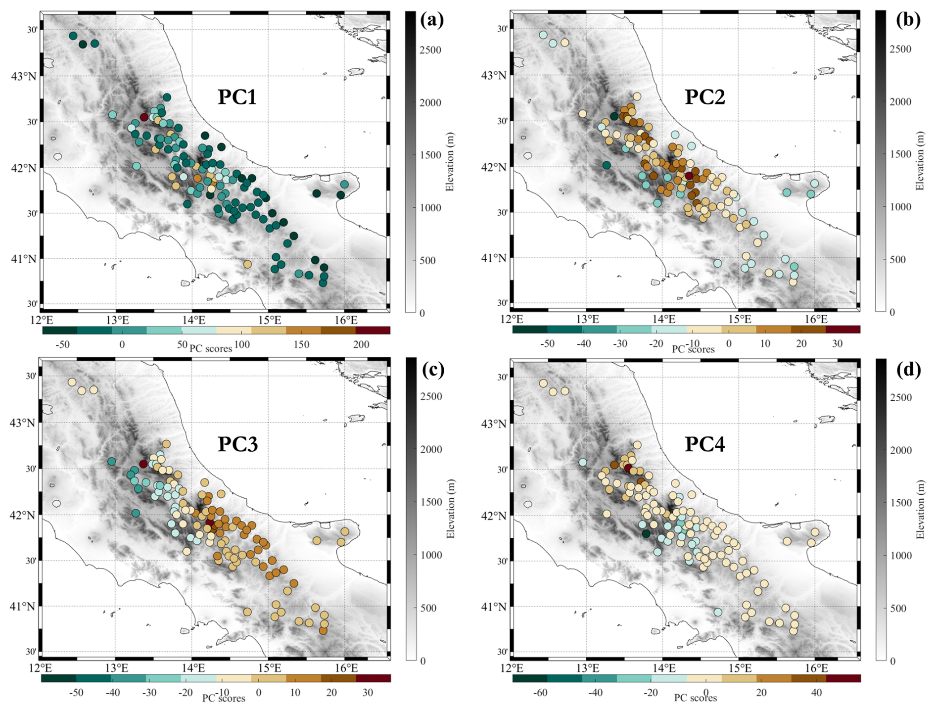
Figure A1 Spatial pattern of the first four modes resulting from the principal component analysis applied to monthly SCD data.

Starting from SCD, the first PC (Fig. A1a), which represents 61 % of the total variance, reflects the altitude-related variability across the whole elevation range. Areas with positive scores coincide with some of the main mountain ridges of the considered region (Gran Sasso, Marsicani, Maiella, and Partenio). Negative scores mark low-elevation areas, as well as the eastern and southern mountain slopes of the central Apennine chain, where the local topographic features are not favourable for the persistence of snow on the ground. More compelling evidence about the relationship between PC1 and elevation is provided in Fig. A2 in which the PC1 scores are plotted against the altitude. A solid positive correlation was found (the linear correlation coefficient, ρ, is equal to 0.87).

Figure A2 First principal component (PC1) scores resulting from the PCA applied to monthly SCD data as a function of the elevation (in m). Each point represents one station.

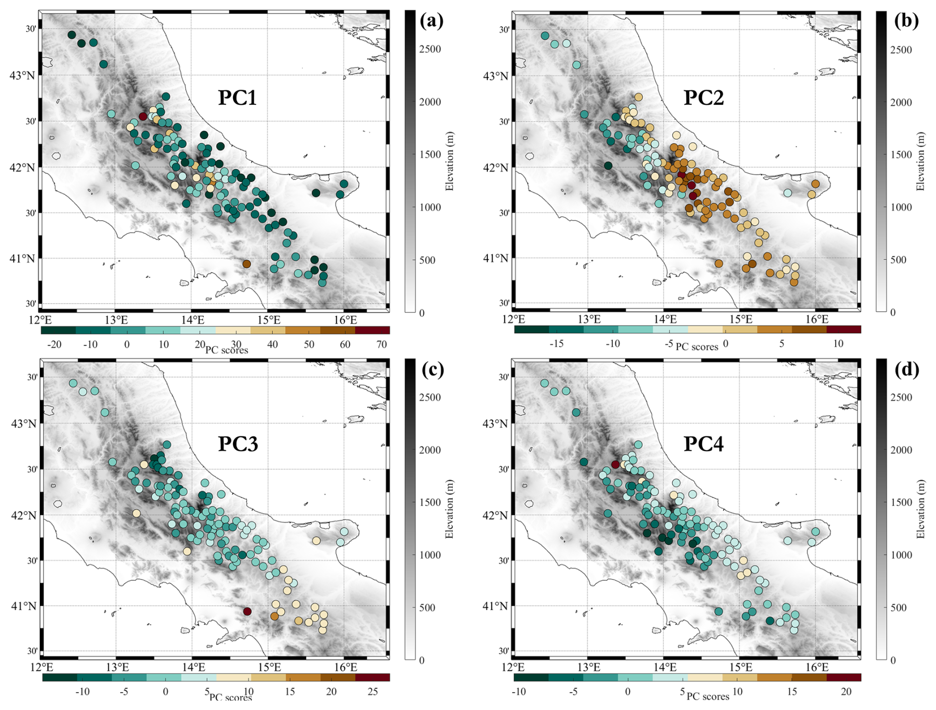
Figure A3 Spatial pattern of the first four modes resulting from the principal component analysis applied to monthly NDS data.

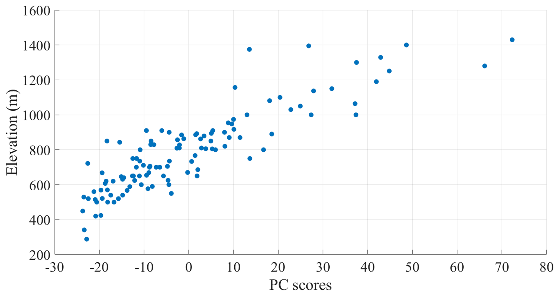
Figure A4 First principal component (PC1) scores resulting from the PCA applied to monthly NDS data as a function of the elevation (in m). Each point represents one station.

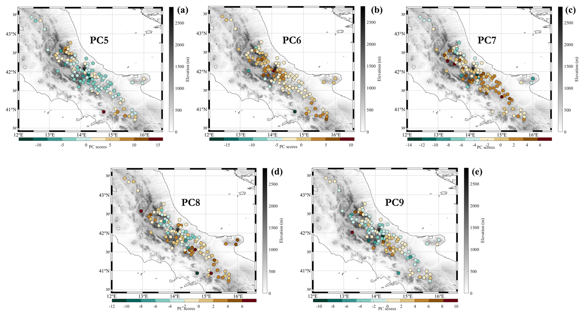
Figure A5 Spatial pattern of the fifth, sixth, seventh, eighth, and ninth mode resulting from the principal component analysis applied to monthly NDS data.

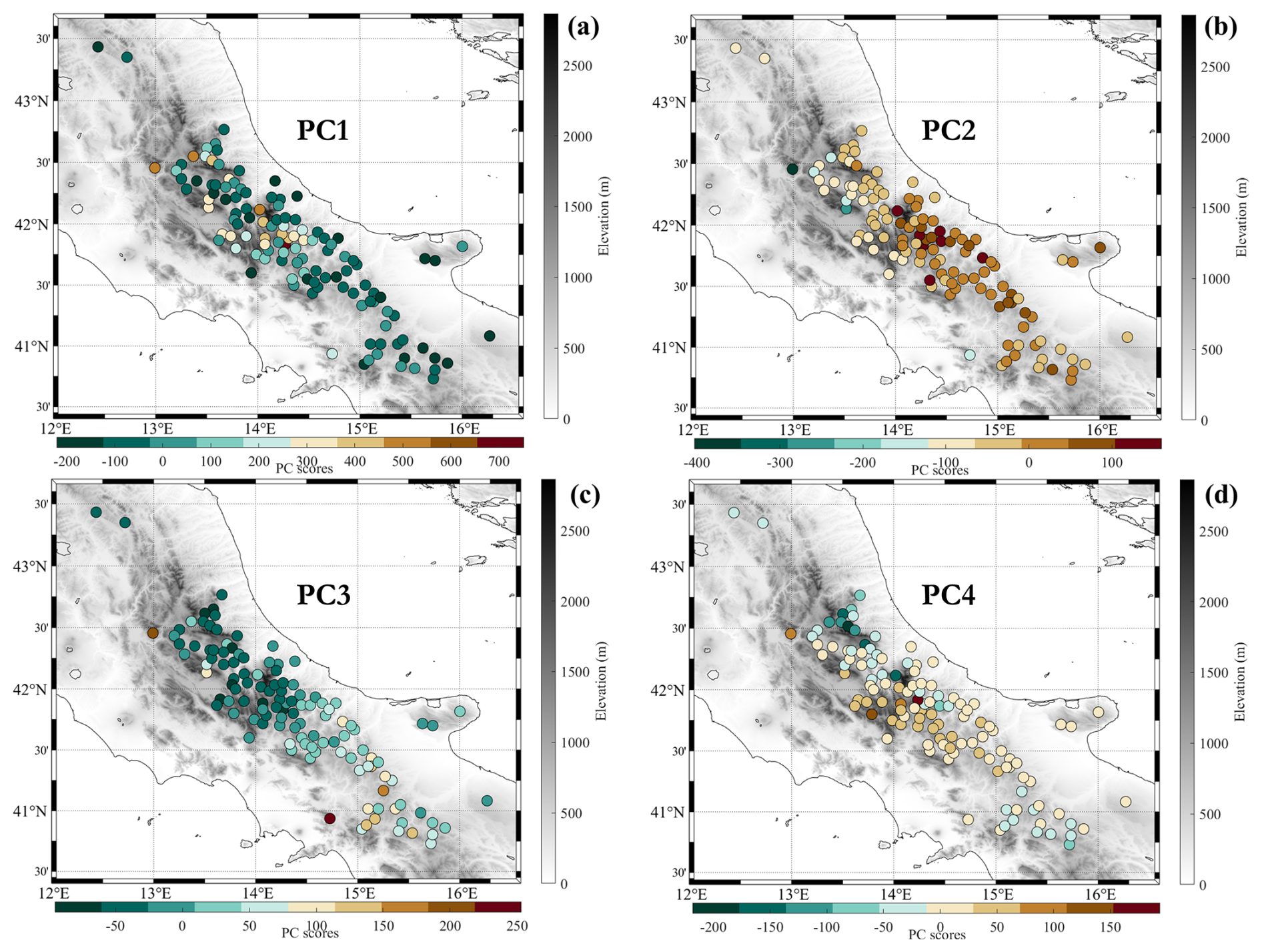
Figure A6 Spatial pattern of the first four modes resulting from the principal component analysis applied to monthly HN data.

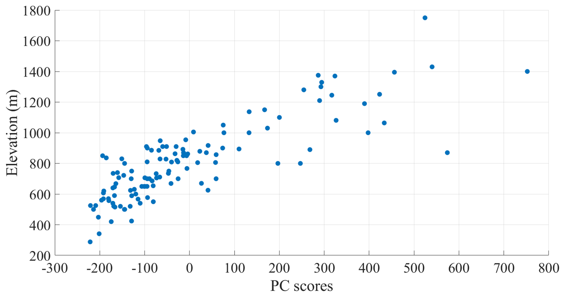
Figure A7 First principal component (PC1) scores resulting from the PCA applied to monthly HN data as a function of the elevation (in m). Each point represents one station.

The PC2 (Fig. A1b) separates the central Apennine sector (Abruzzo and Molise regions) from the southern area. In the first one, the scores are generally positive, whereas in the second one, they are slightly negative. The high positive scores found in several sectors of Abruzzo and Molise (mainly in the Gran Sasso and Marsicani areas) indicate relevant positive SCD anomalies.

The PC3 spatial pattern (Fig. A1c) is characterised by a clear west–east gradient. More specifically, positive scores have been found in the Maiella area, in the eastern side of Marsicani Mountains and in the eastern side of Molise and southern Apennine. In the western sector of Abruzzo region, negative scores prevail instead. This pattern might reflect specific large-scale atmospheric weather regimes, associated with the incoming, over the study region, cold continental air masses from the Balkan Peninsula. Such an atmospheric scenario promotes conditions favourable to the occurrence and persistence of snow on the ground over the eastern slopes of the Apennines.

In the PC4 spatial pattern (Fig. A1d), the scores are generally around 0.0 except for the northern side of Abruzzo (Gran Sasso mountains). This pattern might reflect specific atmospheric conditions that enhance the snow duration on the ground only in the high-elevation sites of the northern Abruzzo region.

For the NDS variable, we have selected the first nine PCs which capture the 70 % of the total variance. According to Fig. A3a, the first PC represents a scenario in which the spatial distribution of the considered parameter is strictly related to the elevation. In this sense, additional evidence comes from Fig. A4, which clearly demonstrates the strong relationship between PC1 scores and elevation (ρ=0.87).

In the PC2 spatial pattern (Fig. A3b), there is a relevant gradient in terms of PC scores in the Abruzzo region. More specifically, the scores gradually switch from negative to positive values moving eastward. Areas with positive scores match with Maiella, Marsicani, Matese, and southern Apennine reliefs (Partenio, Picentini, and Lucania mountains). It may hypothesise that behind this NDS spatial pattern there is a synoptic-scale atmospheric circulation scheme like that described for PC3 of SCD variable, i.e. a configuration associated with the incoming, over the Italian Peninsula, cold air masses from the Balkan region.

In the PC3 spatial pattern (Fig. A3c), the scores are negative over a large part of the study area. Positive values are restricted to the Campania Apennine (Partenio and Picentini mountains). Therefore, this spatial pattern might represent meteorological scenarios in which the snowfall events mainly affect the meridional sector of the considered area.

The PC4 spatial pattern (Fig. A3d) exhibits a spatial structure close to PC2. However, in this case, the zonal gradient is not limited to the Abruzzo region, but it is extended to the whole area. As for PC2, scores gradually increase from west to east, so the largest values have been found on the eastern slopes of the Apennines and over the Gargano area.

The other five selected PCs are presented in Fig. A5. It is worth noting that such spatial patterns represent a very small fraction of variability (2 % for PC5, PC6, PC7, and PC8 and 1 % for PC9), so it is not straightforward to identify a “coherent” behaviour in the spatial distribution of the scores. More specifically, in the PC5 spatial pattern (Fig. A5a), the most relevant positive NDS anomalies occurred in the Gran Sasso area (north of Abruzzo) and in the Campania Apennine (Partenio Mountains). PC6 pattern (Fig. A5b) is close to PC5; however, in this case, positive scores, and so positive NDS anomalies, are confined to the Marsicani mountain area. The PC7 spatial pattern (Fig. A5c) reflects meteorological scenarios that determine positive NDS anomalies over the central and northern sectors of Abruzzo region, namely Molise and Campania Apennine. In the PC8 spatial pattern (Fig. A5d), positive scores are confined to a specific sector of Abruzzo (Gran Sasso and Marsicani mountains) and to the southern sector of Molise. Finally, in PC9, the highest scores are located over the Gran Sasso area, Molise region, and, locally, over the Campania Apennine (Fig. A5e).

The results for the height of the new snow variable (HN) are presented in Fig. A6. Similar to SCD, the first four PCs have been selected. The first PC, accounting for 52 % of the total variance, shows a spatial pattern strongly modulated by the altitude (Fig. A6a). As for SCD and NDS, a strong positive correlation between scores and elevation has been detected (ρ=0.83). However, in this case, the scores associated with stations above 800 m a.s.l. exhibit a great variability (see Fig. A7) due to the relevant incidence of orographic effects on snowfall amounts.

The analysis of the PC2 spatial pattern (Fig. A6b) reveals a clear west–east gradient in the central Apennine area. The large positive scores found over the Maiella area, Marsicani Mountains, Matese, and most of the southern Apennine indicate that such areas receive snowfall amounts that are substantially higher than average, whereas the negative scores over the western side of the Apennines are synonymous with the HN quantity that is near or below average. This spatial pattern can be interpreted as a consequence of large-scale configurations that promote the incoming of cold continental air masses in the central Mediterranean area. In this scenario, central and southern Italy are often affected by a cyclonic area driving a northeastern flow, which enhances orographic precipitation events over the eastern slopes of the Apennines.

In the PC3 spatial pattern (Fig. A6c), the positive scores are concentrated over the southern Apennine, in some areas of Molise, and in the Reatini Mountains. In the Abruzzo region, the scores are generally negative instead. Finally, the PC4 spatial pattern (Fig. A6d) is characterised by large positive scores over the western side of the Marsicani area and the Reatini Mountains. In PC3 and PC4, areas marked with positive scores receive snowfall amounts that are higher than average. Such spatial patterns can be related to specific large-scale weather patterns that modulate the spatial distribution of snow precipitation in the considered region.

Appendix B

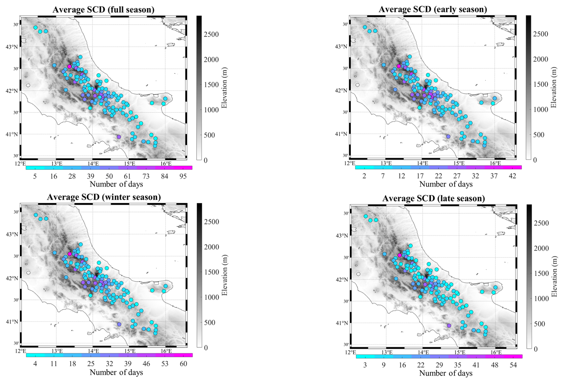
Figure B1 Spatial distribution of the average seasonal snow cover duration (SCD) over the study area in the period 1971–2000. Each point represents one station and the corresponding climatological value.

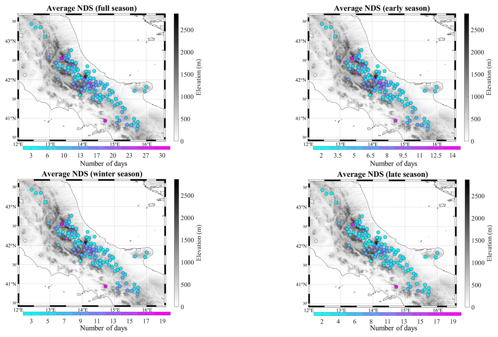
Figure B2 Spatial distribution of the average seasonal number of days with snowfall (NDS) over the study area in the period 1971–2000. Each point represents one station and the corresponding climatological value.

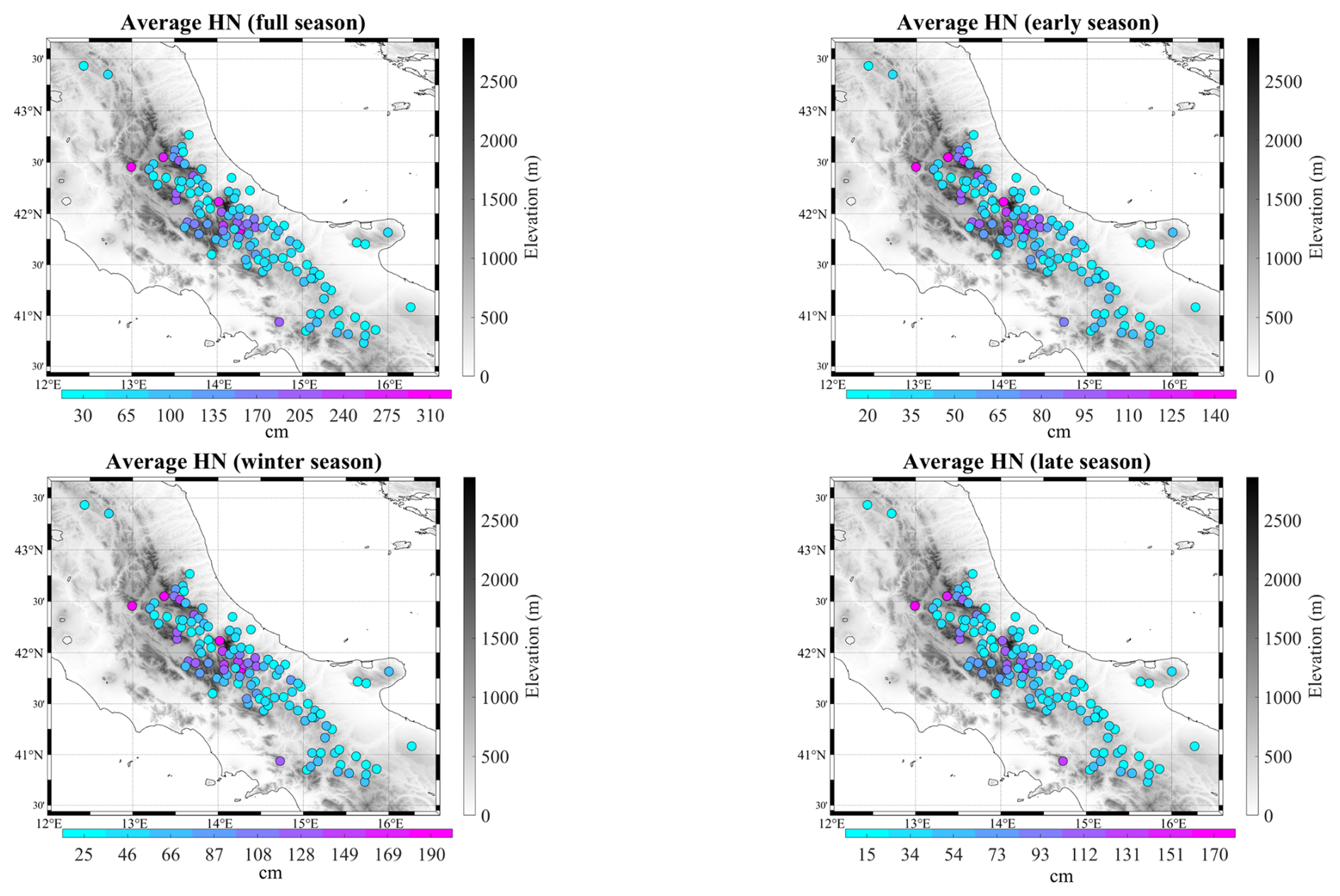
Figure B3 Spatial distribution of the average seasonal total height of new snow (HN) over the study area in the period 1971–2000. Each point represents one station and the corresponding climatological value.