Impact of non-normal flow rule on linear kinematic features in pan-Arctic ice-ocean simulations

The standard sea ice viscous-plastic (VP) rheology is based on an elliptical yield curve and a normal flow rule. This formulation implies that the post-failure deformations are always normal to the yield curve. A drawback of this is that modifications to the yield curve also lead to notable changes to the deformations. We implemented the plastic potential approach of Ringeisen et al. (2021) in the CICE sea ice model. With this formulation, deformations are normal to an elliptical plastic potential which is defined independently from the yield curve. This an interesting capability as it allows to independently optimize deformations while parameters defining the yield curve could serve to adjust landfast ice and to a lesser extent sea ice drift. We investigated the impact of a non-normal flow rule in pan-Arctic simulations. Compared to the standard VP rheology, the non-normal flow rule leads to a more active sea ice cover with narrower linear kinematic features (LKFs) and a higher LKF density. The higher divergence with the non-normal flow rule causes an enhanced ice growth and larger Arctic sea ice volume. In idealized experiments, Ringeisen et al. (2021) showed that the non-normal flow rule can correct the unrealistic (too large) intersection angles between LKFs. However, in our pan-Arctic simulations, the non-normal flow rule does not correct the unrealistic intersection angles which are often around 90°. Results suggest that these frequent 90° angles are partly caused by the alignment of LKFs with the computational grid.

1 Introduction

The yield curve and the flow rule are two important characteristics to define a viscous-plastic (VP) sea ice rheology. The yield curve (e.g. in stress invariant space) specifies the critical stresses associated with the failure of sea ice in shear/compression or shear/tension. The flow rule defines the post-failure deformations. The standard VP rheology of Hibler (1979) is based on an elliptical yield curve and a normal flow rule. With this formulation, the post-failure or plastic deformations are always normal to the yield curve. A limitation of this approach is that modifying the yield curve, for example to optimize simulated landfast ice (e.g., Lemieux et al., 2016), also impacts deformations of the pack ice.

Ringeisen et al. (2021) introduced a plastic potential approach that formulates the flow rule independently from the yield curve. With their formulation, the plastic potential is also defined by an ellipse. As the post-failure deformations are normal to the plastic potential, a non-normal flow rule (with respect to the yield curve) can be obtained.

We have implemented, in the CICE sea ice model, the plastic potential approach of Ringeisen et al. (2021). In this study, we investigate in pan-Arctic experiments the impact of non-normal flow rules on the simulated sea ice cover and especially on linear kinematic features (LKFs). The goal here is not to do a thorough assessment of the realism of simulated LKFs against observations but rather to conduct a sensitivity study of the impact of parameters defining the yield curve and the plastic potential.

The ability of large-scale continuum-based sea ice models to simulate LKFs and more generally deformations was evaluated in the Sea Ice Rheology Experiment (SIREx, Bouchat et al., 2022; Hutter et al., 2022). Various methods and metrics were used to quantify the quality of simulated deformations. These included probability density function (PDF) of deformations, temporal and spatial scaling, LKF density, length of LKFs, intersection angles and LKF lifetime. For most metrics, there were notable differences in the quality of the simulations with some models that performed well while others struggled to properly represent the deformations. However, all the models, whatever the rheology, failed to correctly represent the distribution of intersection angles for pairs of conjugate LKFs (i.e., LKFs that form simultaneously under compressive stresses). Indeed, the peak of the distribution is around 45° for observed deformations (as recently confirmed, Ringeisen et al., 2023) while the models lead to simulated intersection angles with a peak of the PDF around 90° (Hutter et al., 2022).

Prior to SIREx, there were already a few indications that viscous-plastic (VP) models tend to simulate too large intersection angles. Ringeisen et al. (2019) demonstrated in uni-axial loading experiments that the standard VP rheology cannot simulate fracture angles smaller than 60° (i.e., 2×30°). Hutter and Losch (2020) analyzed high-resolution MITgcm pan-Arctic simulations and found that intersection angles are too wide compared to observations with a peak of the distribution around 90°.

Ringeisen et al. (2021) attributed to the normal flow rule the inability of the VP model to simulate small intersection angles. Uni-axial idealized compression experiments with a non-normal flow rule demonstrated that smaller intersection angles, more in line with observations, can be obtained and that the intersection angles of LKFs can be precisely linked to the shape of the yield curve and plastic potential following the Arthur angles (Arthur et el., 1977). Another objective of our study is to investigate if smaller intersection angles can also be simulated in more realistic pan-Arctic experiments when using a non-normal flow rule.

This paper is structured as follow. A brief presentation of the plastic potential and the flow rule is given in Sect. 2. Details about the experimental setup and the methodology are respectively given in Sects. 3 and 4. Results are presented and analysed in Sect. 5. Broader implications are discussed in Sect. 6 while concluding remarks are provided in Sect. 7.

2 The plastic potential and the flow rule

This section provides a short overview of the non-normal flow rule and of the plastic potential for the VP rheology with an elliptical yield curve. More details can be found in Ringeisen et al. (2021).

The yield curve in the VP rheology defines the critical stresses associated with plastic failure. To close the system of equations (.i.e, the constitutive and momentum equations), assumptions have to be made about the post-failure deformations, that is the flow rule. The flow rule can be formulated with the use of a plastic potential. The idea is that post-failure deformations are normal to the plastic potential.

In the original VP rheology of Hibler (1979), the plastic potential is the same as the elliptical yield curve. This leads to a normal flow rule: the post-failure deformations are normal to the yield curve. The constitutive equation can be expressed using ζ and η which are respectively the bulk and shear viscosities (Hibler, 1979). Given the ellipse ratio e of major to minor axes, $\mathit{\eta }=e^{-\mathrm{2}}\mathit{\zeta }$, with ζ expressed as

$$\begin{array}{}\text{(1)}& \mathit{\zeta }={\displaystyle \frac{P(\mathrm{1}+k_{\mathrm{t}})}{\mathrm{2}\mathrm{\Delta }}},\end{array}$$

where P is the ice strength, k_t is a parameter between 0 and 1 that determines tensile strength (König Beatty and Holland, 2010) and $\mathrm{\Delta }={\left[D_{\mathrm{d}}^{\mathrm{2}}+e^{-\mathrm{2}}(D_{\mathrm{t}}^{\mathrm{2}}+D_{\mathrm{s}}^{\mathrm{2}})\right]}^{\mathrm{1}/\mathrm{2}}$ with $D_{\mathrm{d}}={\dot{\mathit{ϵ}}}_{\mathrm{11}}+{\dot{\mathit{ϵ}}}_{\mathrm{22}}$ the divergence, $D_{\mathrm{t}}={\dot{\mathit{ϵ}}}_{\mathrm{11}}-{\dot{\mathit{ϵ}}}_{\mathrm{22}}$ the horizontal tension and $D_{\mathrm{s}}=\mathrm{2}{\dot{\mathit{ϵ}}}_{\mathrm{12}}$ the shearing strain rate. These deformations are defined from the components ${\dot{\mathit{ϵ}}}_{\mathrm{11}}$, ${\dot{\mathit{ϵ}}}_{\mathrm{22}}$ and ${\dot{\mathit{ϵ}}}_{\mathrm{12}}$ of a symmetric strain rate tensor.

Using an elliptical yield curve, Ringeisen et al. (2021) implemented a modified VP rheology that relies on another ellipse defining the plastic potential. Following the notation of Ringeisen et al. (2021), e_F defines the aspect ratio of the yield curve while e_G defines the one of the elliptical plastic potential. With this formulation, η is equal to $e_{\mathrm{G}}^{-\mathrm{2}}\mathit{\zeta }$. The bulk viscosity ζ is in this case expressed as in Eq. (1) above but with a slight modification to the definition of Δ, that is

$$\begin{array}{}\text{(2)}& \mathrm{\Delta }={\left[D_{\mathrm{d}}^{\mathrm{2}}+{\displaystyle \frac{e_{\mathrm{F}}^{\mathrm{2}}}{e_{\mathrm{G}}^{\mathrm{4}}}}(D_{\mathrm{t}}^{\mathrm{2}}+D_{\mathrm{s}}^{\mathrm{2}})\right]}^{\mathrm{1}/\mathrm{2}}.\end{array}$$

Setting $e_{\mathrm{G}}=e_{\mathrm{F}}=e=\mathrm{2}$, one recovers the VP rheology introduced by Hibler (1979). Note that there is a sign that is incorrect in the definition of Δ in Ringeisen et al. (2021, their Eq. 15).

When the deformation Δ tends toward zero, ζ tends toward infinity. To prevent this singularity, Δ is replaced by Δ^* in Eq. (1). In the simulations presented in this article, Δ^* is defined by the capping approach of Hibler (1979), that is ${\mathrm{\Delta }}^{*}=max(\mathrm{\Delta },{\mathrm{\Delta }}_{min})$, where Δ_min is a small deformation set here to 10⁻¹¹ s⁻¹.

As only small modifications to the definitions of η and Δ are required, the implementation of the non-normal flow rule for the VP rheology with an elliptical yield curve is straightforward. There is also no impact on the computational efficiency. The supplement of this article describes the idealized numerical experiments that were conducted to validate our implementation of the plastic potential and non-normal flow rule. Results demonstrate that a VP solution is still obtained when e_G≠e_F (for both implicit and explicit elastic-VP (EVP) approaches). Moreover, simulated fracture angles in uni-axial compression experiments are close to the theoretical values and the ones obtained by Ringeisen et al. (2021).

3 Experimental setup

Our experimental setup is based on the CICEv6.5 sea ice model (Hunke et al., 2023) and the NEMOv3.6 ocean model (Madec, 2008). CICEv6.5 includes both B and C-grid discretizations. The B-grid discretization is used here. We use a regional configuration with a domain that covers the Arctic Ocean, the oceanic regions around Canada, the North Atlantic and the North Pacific. This setup was developed as part of the Canadian Operational Network of Coupled Environmental Prediction Systems (CONCEPTS) initiative. The regional grid for the simulations is the CONCEPTS REGional $\mathrm{1}/\mathrm{12}$° (CREG12) grid which is used in the Environment and Climate Change Canada (ECCC) operational regional ice ocean prediction system (RIOPS, Smith et al., 2021).

The ocean model is applied in a variable volume and nonlinear free surface formulation, using seventy-five vertical levels. Ocean mixing is parameterized with the NEMO k-epsilon approach. Oceanic boundary conditions for the North Pacific and North Atlantic are taken from the GLORYS2 version 4 reanalysis (Garric et al., 2017). Monthly averages of vertical profiles of ocean currents, temperature, and salinity are applied at the boundaries. A time-splitting technique with a sub-time step of 5 s is used for the treatment of the nonlinear free surface (including the tides). For the tides, vertically averaged velocities (13 harmonic components) were obtained from the Oregon State University tidal prediction model. At the open boundaries, the barotropic part of the velocity components are prescribed following the method of Flather (1976). Sea surface height forcing includes the tidal potential, self-attraction and loading effects.

Ten sea ice thickness categories, as defined in Smith et al. (2016), are used for the simulations. The thermodynamics component uses the approach of Bitz and Lipscomb (1999). The parameterization of Hibler (1979) is employed for the formulation of the ice strength. For most of the simulations, the EVP method is used for solving the momentum equation (Hunke, 2001). Grounding of ice keels in shallow water is parameterized with the scheme of Lemieux et al. (2016).

The ice-ocean simulations are forced by 33 km resolution ECCC atmospheric reforecasts (Smith et al., 2014). As the ECCC atmospheric forcing dataset only covers the period from 2001 to 2010, this puts some constraints on the spinup and analysis period. The analysis period is 25 September 2004 to 31 May 2008. The restart on 25 September 2004 was produced following the method described in Lemieux et al. (2018). It was obtained from a CICEv4-NEMOv3.6 simulation consisting of a pseudo-spinup followed by a final spinup.

The pseudo-spinup was initialized with average (September–October 2001) sea ice concentration from the National Snow and Ice Data Center (NSIDC, https://nsidc.org/data/seaice_index/, last access: 4 November 2025) and the average (October–November 2003) sea ice thickness field from ICESat data (https://nsidc.org/data/icesat, last access: 4 November 2025). The initial temperature and salinity for the ocean are averages (September–October) of WOA13_95A4 fields (Locarnini et al., 2013; Zweng et al., 2013). The ocean started at rest; the sea surface height field and ocean currents were set to zero. The pseudo-spinup consisted in running the coupled model three times from 1 October 2001 to 30 September 2002.

The pseudo-spinup solution was then used to start the spinup again on 1 October 2001. CICEv4-NEMOv3.6 then ran up to 25 September 2004. The solution on 25 September 2004 is the restart that is used for the simulations. The sea ice part of the restart was converted in order to be used by CICEv6.5.

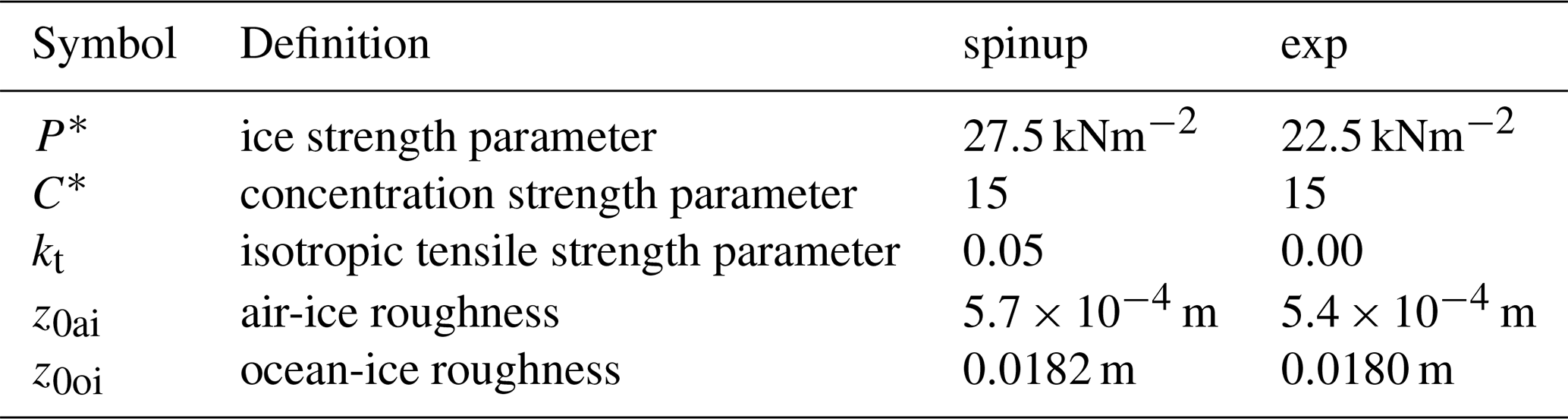
For the pseudo-spinup and the spinup, we used the “optimal” parameters of Chikhar et al. (2019). Table 1 lists the values of the most relevant parameters for the spinup procedure, that is the ones associated with rheology and sea ice dynamics (note that e = 1.5 for the pseudo-spinup and spinup). The advective time step is 180 s for the spinup procedure and for all the simulations. Following the advice of Bouchat et al. (2022), a large number (900) of EVP subcycles were performed in order to ensure numerical convergence of the solutions.

Table 1 Relevant dynamical parameters for the spinup (and pseudo-spinup) and for the numerical experiments.

4 Methodology

4.1 Sensitivity analysis

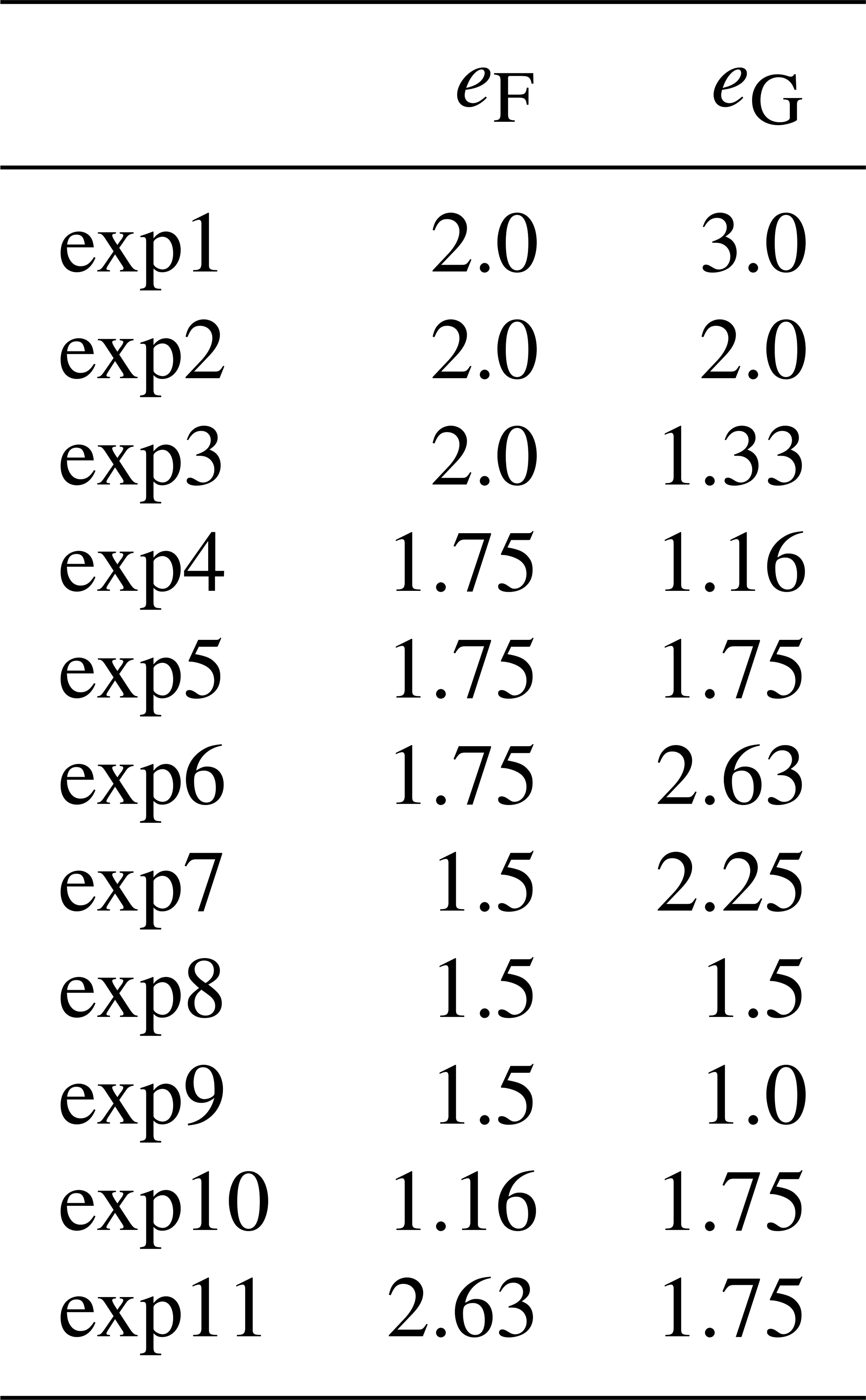
From the ice-ocean restart described in Sect. 3, we ran a series of numerical experiments with different values of e_F and e_G. To simulate smaller intersection angles, Ringeisen et al. (2021) suggest to set e_G<e_F. Nevertheless, as this is a sensitivity study, we also test for values of e_G larger than e_F keeping in mind that the most important results are for e_G<e_F. For each value of e_F, e_G is set to $\sim e_{\mathrm{F}}/\mathrm{1.5}$ or e_F or ∼1.5e_F (these are referred to experiments 1 to 9). As e_F=1.75 is between the two other values tested (i.e., e_F=1.5 and e_F=2.0), we sometimes only show results associated with this value when the conclusions are qualitatively the same for the other values of e_F. We add two other experiments to see the impact of e_F for a constant e_G of 1.75 (referred to as experiments 10 and 11). The values of e_F and e_G for the 11 numerical experiments are given in Table 2. Except for $C^{*}=\mathrm{15}$, the other dynamical parameters for the experiments are slightly different than the ones used for the spinup procedure. P^*, z_0ai and z_0oi are set to the values of the latest version of RIOPS (Smith et al., 2021). As in Ringeisen et al. (2021), k_t is set to zero. The last column of Table 1 provides the values of these parameters. Again, the number of EVP subcycles is set to 900.

Table 2 List of numerical experiments with values of e_F and e_G.

These experiments cover the period 25 September 2004 to 31 May 2008. We are interested in the formation of LKFs when the sea ice is compact in the Arctic Ocean. We therefore analyse the LKFs between 1 January to 31 May for the years 2005 to 2008. We focus our analysis on the first winter-spring period (i.e., 2005) because the sea ice thickness fields of the different simulations are more similar. Nevertheless, we also analyze LKF statistics for the other winter-spring periods to verify that the same conclusions apply. We use 00:00 UTC snapshots of sea ice deformations to investigate the simulated LKFs. Daily mean of the sea ice volume were also stored to study the impact of the non-normal flow rule on total sea ice volume in the northern hemisphere.

4.2 LKF detection and analysis

To detect LKFs, we downloaded version 2.0 of Nils Hutter's LKF package (https://github.com/nhutter/lkf_tools/releases/tag/v2.0, last access: 4 November 2025, Hutter et al., 2019) and made a few minor modifications for our CICE outputs. LKFs are detected only if the sea ice concentration is larger than 0.15 and if they are located in a region in the central Arctic defined by a mask. We refer to this mask as the pack ice mask. It covers the region shown in gray in Fig. 1. It corresponds to all the CREG12 grid cells in the Arctic Ocean that are at least 250 km away from the nearest land cell. This mask ensures that LKFs are detected and analysed in compact ice, away from the coasts and from regions of landfast ice (i.e. excluding coastal or flaw polynyi).

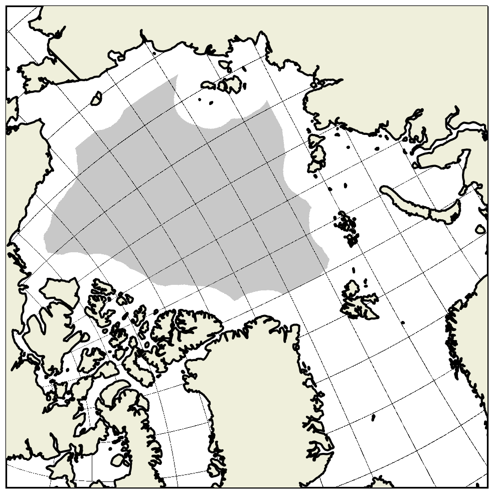
Figure 1 The gray region displays the mask used for the detection of LKFs in pack ice. The thin black lines show the orientation of the grid axes. Given the grid indices i and j, the grid axes are plotted for $i=\mathrm{100},\mathrm{200},\mathrm{300}\mathrm{\dots }$ and similarly for $j=\mathrm{100},\mathrm{200},\mathrm{300}\mathrm{\dots }$

We analyse spatial characteristics of LKFs and leave aside temporal aspects such as the lifetime of LKFs. To analyse the detected LKFs, we developed a set of tools written in Python. These tools can be obtained on GitHub (https://github.com/JFLemieux73/lkf_tools, last access: 4 November 2025). Many of the metrics used to analyse the LKFs are the same ones introduced in Hutter and Losch (2020) and Hutter et al. (2022). However, we introduce two new metrics: the width of LKFs and the angle with the grid.

The detection algorithm uses a morphological thinning method that reduces the width of LKFs to one pixel (Hutter et al., 2019). A kernel value of seven was used for the detection algorithm. In the most recent implementation, a point of a thinned LKF corresponds to the largest total deformation along a perpendicular transect (Hutter, 2023). Given the location of a LKF point with a total deformation of ${\dot{\mathit{ϵ}}}_{\mathrm{tot}}$, our new Python algorithm calculates the number of pixels (i.e., grid cells) required in both perpendicular search directions for reducing the total deformation below $\mathit{\alpha }{\dot{\mathit{ϵ}}}_{\mathrm{tot}}$ where $\mathrm{0}<\mathit{\alpha }<\mathrm{1}$. The parameter α is set to 0.5 in this study. More details about the LKF width algorithm are provided in Appendix A.

Our LKF analysis tool also estimates angles of LKFs with the computational grid at the intersection points of conjugate LKFs. As such, it first identifies pairs of intersecting LKFs. Following Hutter et al. (2022) and Ringeisen et al. (2023), the vorticity of both intersecting LKFs is analysed. If the two LKFs have opposite signs of vorticity, the intersecting pair can be interpreted as conjugate LKFs. As shown in Fig. B1 in Hutter et al. (2022), the stress direction can be determined from the vorticity field; the intersection angle obtained is between 0 and 180°. For each intersecting LKF, our Python tool then calculates the acute angles θ_x and θ_y between a LKF and the (local) x and y axis of the computational grid. The metric that we use is the minimum angle with the grid, that is ${\mathit{\theta }}_{\min }=min({\mathit{\theta }}_x,{\mathit{\theta }}_y)$. More details about our algorithm for calculating intersection angles and angles with the grid are given in Appendix B.

4.3 Spatial scaling

As a complement to the LKF metrics described above, we investigate the spatial scaling response to the plastic potential. This metrics is not a direct measure of the organization of sea ice deformations into LKFs but measures the level of spatial localization of the simulated deformations. While not as intuitive as the LKF characteristics, this metric has the benefit of being independent from the LKF detection methods, thus generalizing the results.

The spatial scaling is performed by applying the same coarse-graining methods as described in Bouchat and Tremblay (2020) and Bouchat et al. (2022), but here applied to Eulerian sea ice deformations (i.e., without the initial step of computing Lagrangian trajectories, Hutter et al., 2018). That is, for a given coarsened scale L, the mean sea ice deformation is computed first by aggregating to scale the Finite Difference sea ice velocity gradients (using an area-weighted average), then computing the field-average of these coarse-grained deformations. This method is repeated across multiple scales (multiples of the nominal resolution), and the spatial scaling is defined by the slope β of the regression line in logarithmic space that best represents the results.

Following Bouchat and Tremblay (2020) and Bouchat et al. (2022), the aggregated sea ice deformations are further weighted by their signal-to-noise ratio. This method was designed to apply similar post-processing methods to model data as those applied to satellite observations, with the added benefit of presenting an enhanced sensitivity to the level of feature localization. This method is adapted to our Eulerian approach by setting the tracking error to zero and the sea ice velocity error to the model precision, yielding a unique noise value for all deformations. The signal-to-noise weighting method therefore corresponds to weighting the sea ice deformations by their own magnitude.

4.4 Ratio of divergence and shearing

Because the post-failure deformations are normal to the plastic potential, a simulation with a large value of e_G should exhibit less convergence/divergence and more shear than a simulation with a smaller value of e_G. To investigate the impact of the plastic potential on the post-failure deformations, the amount of divergence compared to shear is quantified by calculating

$$\begin{array}{}\text{(3)}& {\mathit{\theta }}_r={\tan }^{-\mathrm{1}}\left({\displaystyle \frac{{\dot{\mathit{ϵ}}}_{\mathrm{I}}}{{\dot{\mathit{ϵ}}}_{\mathrm{II}}}}\right),\end{array}$$

where ${\dot{\mathit{ϵ}}}_{\mathrm{I}}=D_{\mathrm{d}}$ and ${\dot{\mathit{ϵ}}}_{\mathrm{II}}=(D_{\mathrm{t}}^{\mathrm{2}}+D_{\mathrm{s}}^{\mathrm{2}}{)}^{\mathrm{1}/\mathrm{2}}$ are the strain rate invariants. The angle θ_r varies between −90° (pure convergence) to 90° (pure divergence) with pure shear deformation corresponding to θ_r=0°.

This metric is calculated from 00:00 UTC snapshots of ${\dot{\mathit{ϵ}}}_{\mathrm{I}}$ and ${\dot{\mathit{ϵ}}}_{\mathrm{II}}$. Note that ${\dot{\mathit{ϵ}}}_{\mathrm{I}}$ and ${\dot{\mathit{ϵ}}}_{\mathrm{II}}$ are defined at the T point (i.e., cell center) in the CICE outputs.

5 Results

5.1 Impact of non-normal flow rule on simulated LKFs

Snapshots of the total deformation show that e_G has a strong impact on the definition of LKFs. This is shown in Fig. 2 for 25 April 2005 for which e_F is kept constant at 1.75. For e_G=2.63 (Fig. 2a), LKFs are blurry and not well defined. LKFs are better defined as e_G is reduced (Fig. 2b and c). As e_G is reduced, the algorithm detects more LKFs for these very same snapshots (Fig. 3).

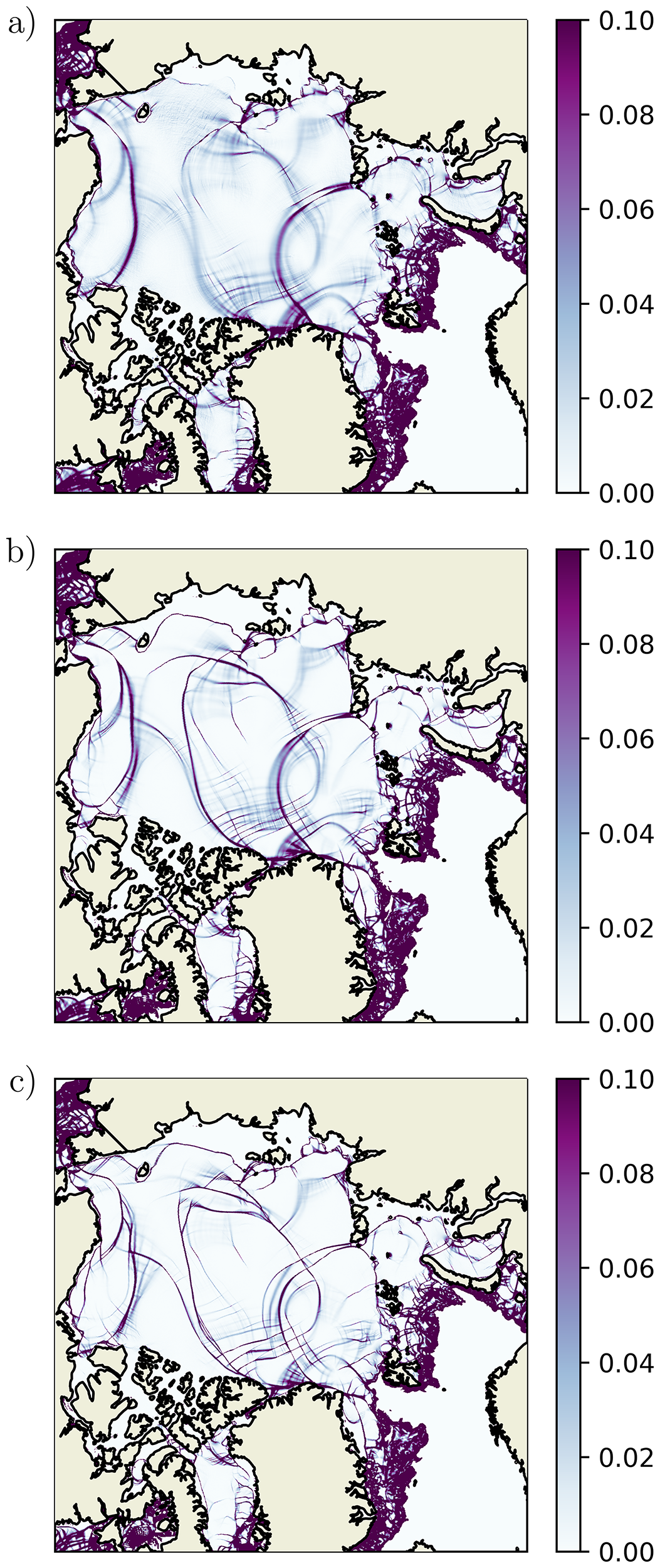
Figure 2 Total deformation in d⁻¹ on 25 April 2005 for e_F=1.75 and e_G=2.63 (a), e_G=1.75 (b) and e_G=1.16 (c). Deformations are not displayed for a concentration smaller than 0.15.

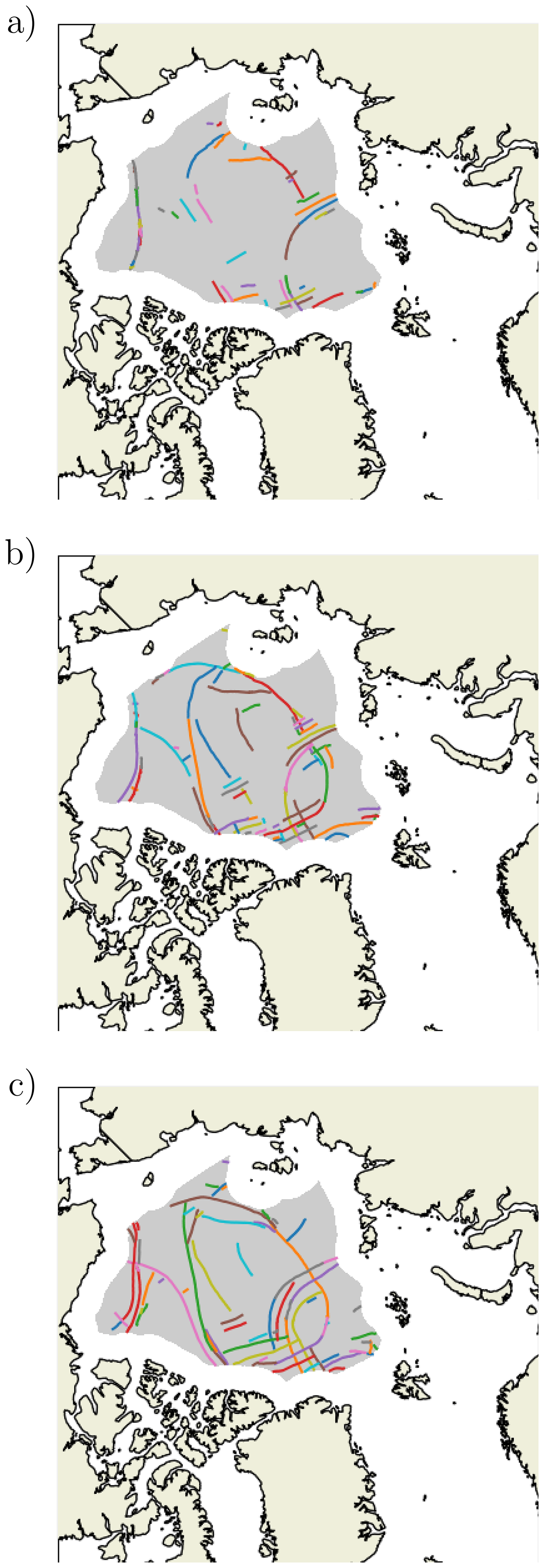
Figure 3 Detected LKFs on 25 April 2005 for e_F=1.75 and e_G=2.63 (a), e_G=1.75 (b) and e_G=1.16 (c). The Arctic mask defining the region for the LKF detection is clearly visible in these panels.

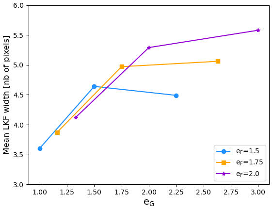
Visually speaking, Fig. 2 shows that similar large-scale patterns of deformation are present for different values of e_G. However, these panels indicate that a smaller e_G leads to narrower LKFs. To verify this, we used our novel Python tool for calculating the width of detected LKFs (see Appendix A for details). The mean width of detected LKFs in the pack ice region over the period 1 January to 31 May 2005 is indeed sensitive to the value of e_G (see Fig. 4). For all the values tested of e_F, a non-normal flow rule with e_G<e_F leads to narrower LKFs compared to the normal flow rule (i.e., e_G=e_F).

Figure 4 Mean width of detected LKFs for the period 1 January to 31 May 2005.

Because LKFs are blurry for large values of e_G (Fig. 2a), the number of detected LKFs is smaller. This is shown in Fig. 5 for e_F=1.75. The mean number of detected LKFs over the period 1 January to 31 May 2005 is 63.2 for e_G=2.63, 86.2 for e_G=1.75 and 106.5 for e_G=1.16. These conclusions remain valid for the other values of e_F (and associated e_G) tested and for the other winter-spring periods (2006–2008) of the simulations (not shown).

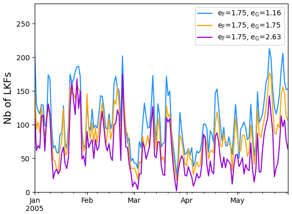
Figure 5 Number of detected LKFs as a function of time for the period 1 January to 31 May 2005.

Detected LKFs also tend to be longer for a smaller e_G. This is clearly displayed in Fig. 6. The increase in the mean length is more pronounced going from e_G= 2.63 to e_G= 1.75 than from e_G=1.75 to e_G= 1.16. The length of a detected LKF was obtained by summing the distances between two neighboring points. These distances were calculated with the haversine formula. The mean length over the period 1 January to 31 May 2005 is respectively 167.4, 221.7 and 257.4 km for e_G= 2.63, e_G= 1.75 and e_G= 1.16. These conclusions remain valid for the other values of e_F (and associated e_G) tested and for the other winter-spring periods (2006–2008) of the simulations (not shown). Because a smaller e_G leads to longer and more numerous LKFs, the total length of LKFs is also larger (see Fig. 7). The mean total length over the period 1 January to 31 May 2005 is respectively 10 739, 18 746 and 26 546 km for e_G= 2.63, e_G= 1.75 and e_G= 1.16.

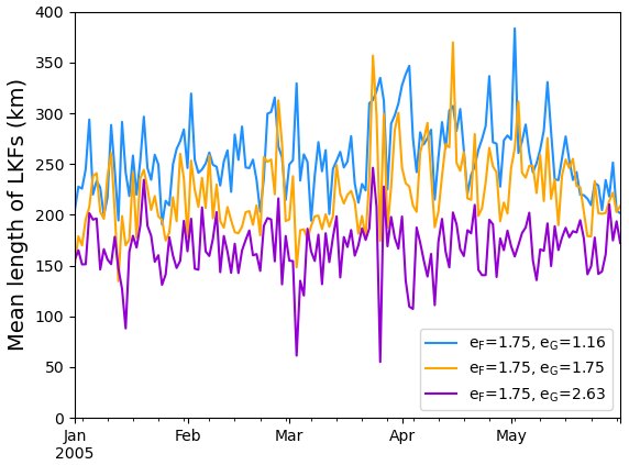
Figure 6 Mean length in km of detected LKFs as a function of time for the period 1 January to 31 May 2005.

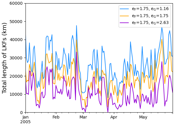
Figure 7 Total length in km of detected LKFs as a function of time for the period 1 January to 31 May 2005.

The more numerous simulated LKFs when decreasing the value of e_G is an ubiquitous phenomenon in the region defined by our pack ice mask as demonstrated by the LKF density maps in Fig. 8. Given the n_s=151 snapshots (00:00 UTC) for the period 1 January to 31 May 2005 that were used for the LKF detection, the density is calculated as the number of incidences a pixel is crossed by a LFK divided by n_s. The density clearly increases as e_G is reduced. These conclusions remain the same for the other values of e_F tested (not shown).

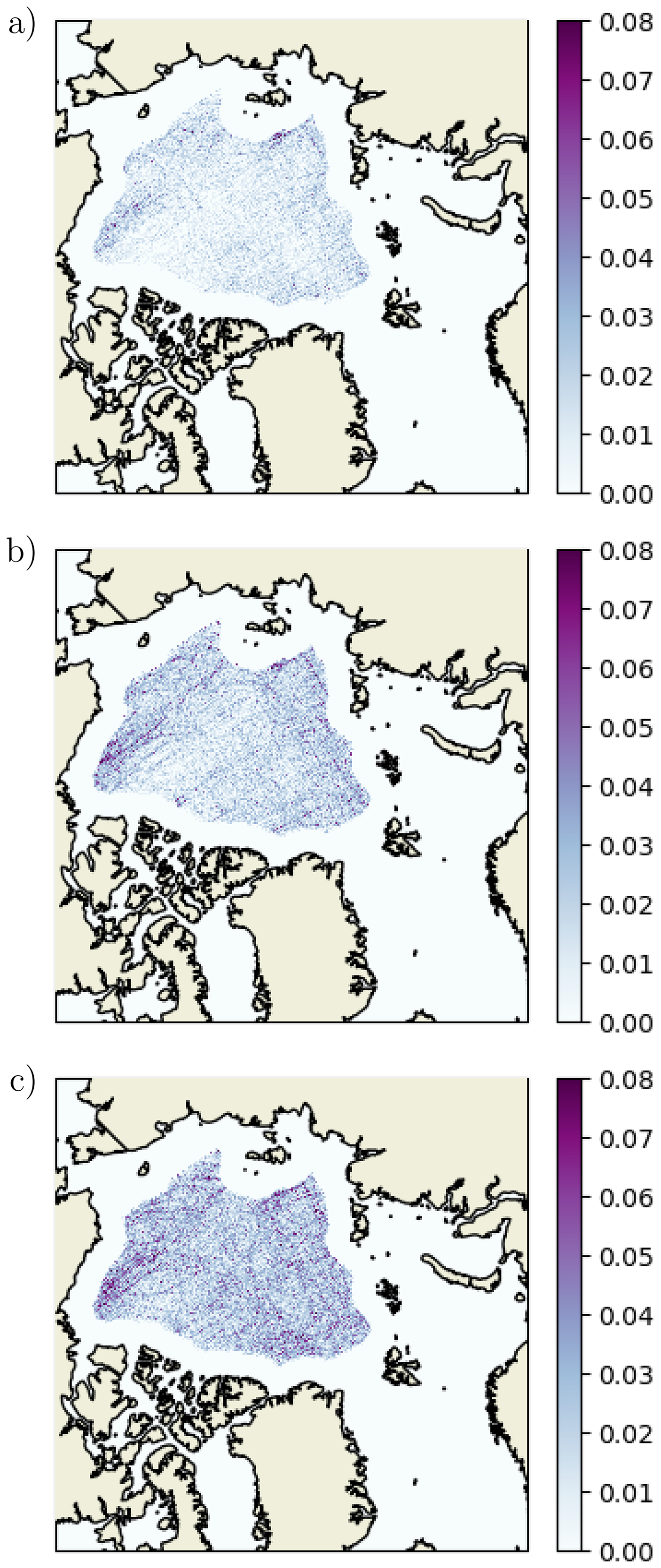
Figure 8 LKF density for the period 1 January to 31 May 2005 for e_F=1.75 and e_G=2.63 (a), e_G=1.75 (b) and e_G=1.16 (c).

One limitation of the LKF metrics discussed above is that they do not consider the smoother or shorter features excluded by the LKF detection algorithm (see for instance the features in Fig. 2a in the region of the pack ice mask vs. the LKFs detected in Fig. 3a). As such, these metrics are likely unable to capture the model sensitivity at high e_G values. This might explain the ambiguous impact of e_G>e_F on the mean LKF width (Fig. 4). To generalize the results and characterize the level of localization in the full sea ice deformation fields, we additionally calculated the spatial scaling from the nominal (∼ 4 km) to ∼ 500 km scales (Fig. 9). This exercise confirms that the level of localization in the simulated sea ice deformation fields is sensitive to e_F but mostly sensitive to the e_G parameter, with increased scaling (larger scaling exponent β) for lower e_G.

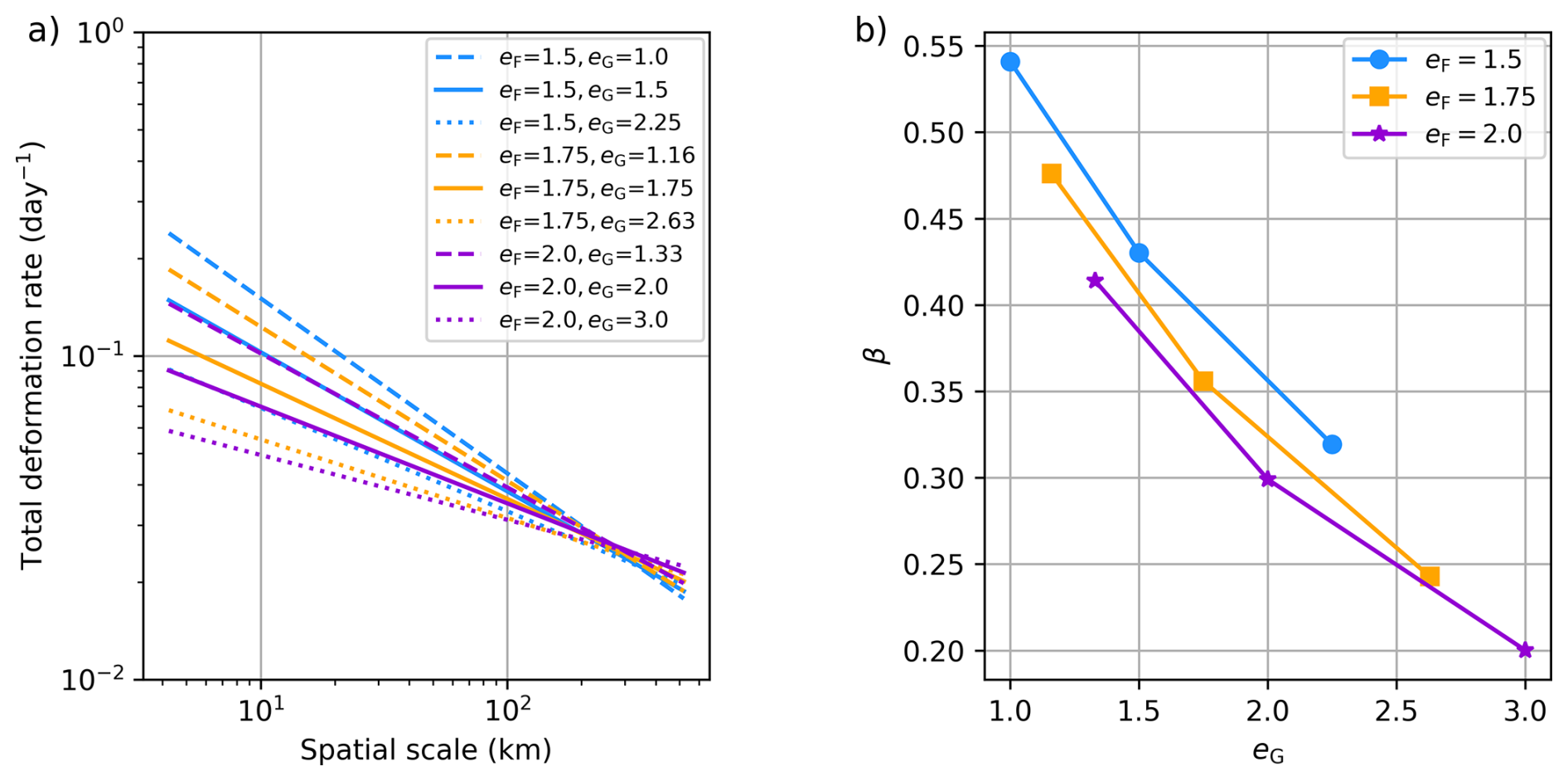
Figure 9 Spatial scaling of the total deformation rates for each of the main experiments (a) and corresponding scaling exponents as function of e_G (b), for the period 1 January to 31 May 2005.

5.2 Impact of non-normal flow rule on intersection angle

In idealized uni-axial compressive experiments on a C-grid, Ringeisen et al. (2021) demonstrated that, compared to e_G=e_F (the normal flow rule case), a plastic potential with e_G<e_F leads to smaller intersection angles between conjugate LKFs for e_F>1. Using a B-grid discretization, we repeated the experiments of Ringeisen et al. (2021) and arrived at the same conclusions (see supplement). Here, we investigate the impact of non-normal flow rules on the intersection angles between conjugate LKFs in pan-Arctic simulations. Details about our Python algorithm for calculating the angle between conjugate LKFs (and angles with the grid) are provided in Appendix B.

Figure 10b shows the PDF of intersection angles for pairs of conjugate LKFs (i.e., θ_c), for the period 1 January to 31 May 2005, for $e_{\mathrm{G}}=e_{\mathrm{F}}=\mathrm{1.75}$. Note that short LKFs are excluded from this analysis; the intersection is not taken into account in the PDF if at least one of the two intersecting LKFs has less than N_min= 10 points. The peak of the distribution is at 90°. This is unrealistic compared to observations of intersection angles (Hutter and Losch, 2020; Hutter et al., 2022; Ringeisen et al., 2023). Reducing (Fig. 10c) or increasing (Fig. 10a) e_G does not improve the PDF. The PDFs in Fig. 10 are similar to the ones obtained by Hutter et al. (2022) for SIREx.

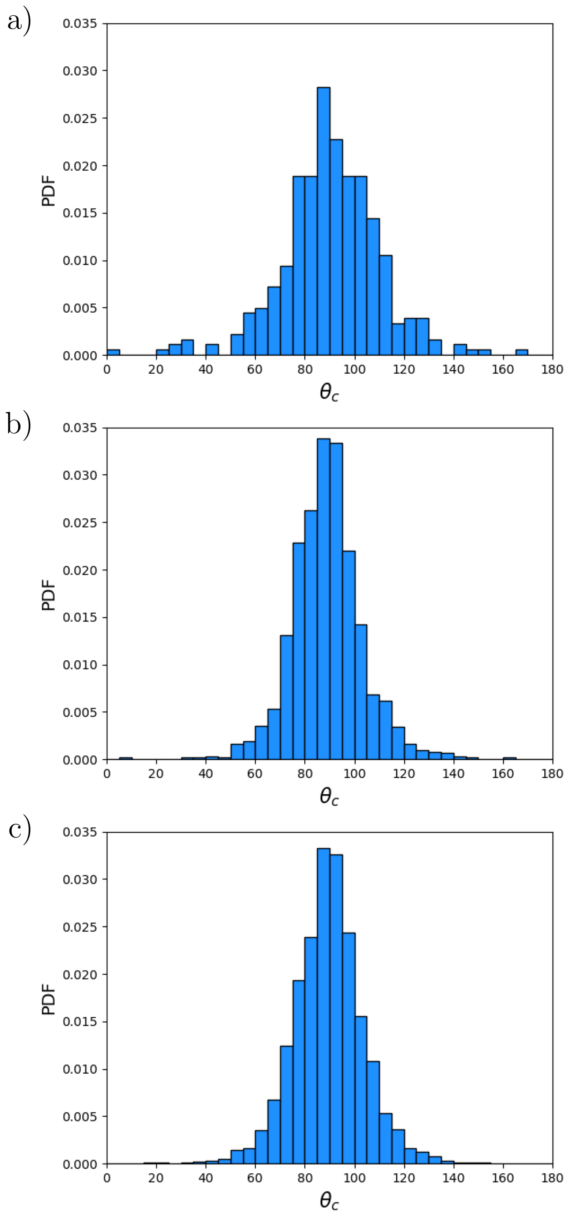
Figure 10 PDF of θ_c, the intersection angle of conjugate LKFs, for e_F=1.75 and e_G=2.63 (a), e_G=1.75 (b) and e_G=1.16 (c). The PDF is calculated from daily snapshots at 00:00 UTC for the period 1 January to 31 May 2005.

Contrary to the results of Ringeisen et al. (2021) for idealized uni-axial compression experiments (and our results in the supplement), the angles between conjugate LKFs are not reduced when setting e_G<e_F in our pan-Arctic simulations (see Fig. 10). As an aside, we also investigated if an implicit approach for solving the momentum equation in these pan-Arctic experiments would produce results in line with the idealized experiments. To do so, we made use of a new capability of CICE: a Picard implicit solver similar to the one developed by Lemieux et al. (2008). The implicit solver in CICE relies on the same spatial discretization as the B-grid EVP (Hunke and Dukowicz, 2002). Using 10 nonlinear iterations for the implicit solver, we ran experiments for $e_{\mathrm{G}}=e_{\mathrm{F}}=\mathrm{1.75}$, $e_{\mathrm{G}}=\mathrm{1.16},e_{\mathrm{F}}=\mathrm{1.75}$, and $e_{\mathrm{G}}=\mathrm{2.63},e_{\mathrm{F}}=\mathrm{1.75}$. PDFs of the intersection angle of conjugate LKFs resemble the ones obtained with the EVP: the peaks are also at 90° for the three experiments (not shown).

As the peaks of all these distributions are close to 90°, one might consider that many LKFs are aligned with the computational grid. Hutter and Losch (2020) briefly investigated this in their MITgcm simulations by comparing the mean orientation of LKFs with grid orientation and could not find a clear correlation. Hutter et al. (2022) also argued that the peak at 90° is not due to LKFs aligned with the grid because SIREx simulations from unstructured grid models also exhibit a peak of the PDF close to 90°.

However, a visual inspection of our simulated deformation fields indicates that many LKFs are aligned with the grid. For example, in Fig. 2, there are many LKFs north of Greenland that intersect at ∼ 90° and that are closely aligned with the grid. The orientations of these LKFs can be compared to the orientation of the grid axes in Fig. 1. To investigate this more objectively, we used our novel Python tool that calculates the angles of LKFs with the (local) x and y axis of the grid. The angles θ_x and θ_y with the x and y axis are calculated at the intersection point of conjugate LKFs. Fig. 11 shows the PDFs of the minimum angle ${\mathit{\theta }}_{\min }=min({\mathit{\theta }}_x,{\mathit{\theta }}_y)$ of all the conjugate LKFs for the period 1 January to 31 May 2005. Given e_F=1.75, the peak of the PDF is clearly at 0° for the three values of e_G tested (Fig. 11). Although decreasing e_G slightly modifies the PDF toward more uniform values, there is still clearly a tendency for LKFs to align (or nearly align) with the computational grid. Due to the continents and large-scale sea ice drift patterns, the same PDF calculated using observed LKFs would not necessarily be uniform.

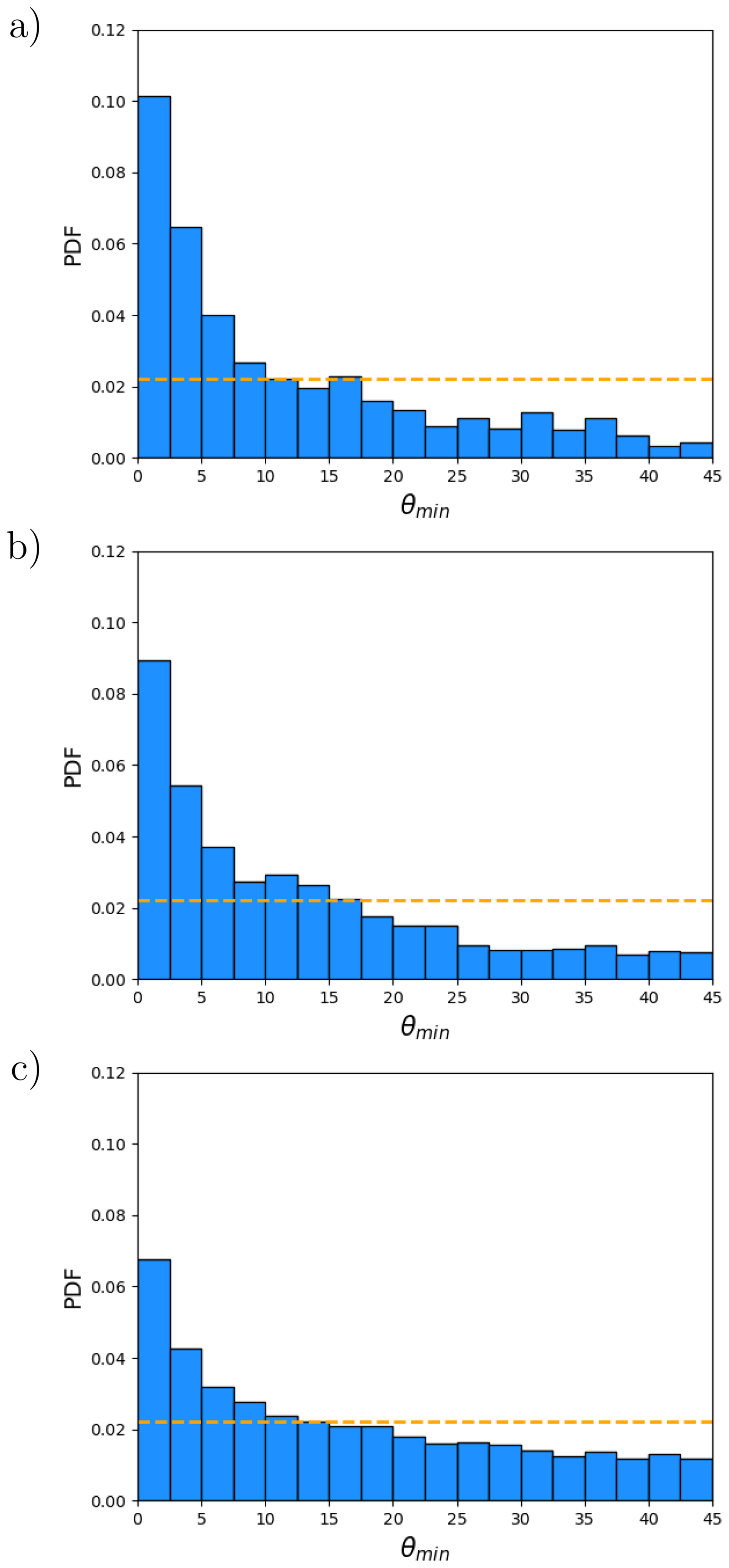
Figure 11 PDF of θ_min, the minimum angle between detected conjugate LKFs and the x and y axis for e_F=1.75 and e_G=2.63 (a), e_G=1.75 (b) and e_G=1.16 (c). The angles are calculated at the intersection point of a pair of conjugate LKFs. The PDF is calculated from daily snapshots at 00:00 UTC for the period 1 January to 31 May 2005. The orange dashed line shows what would be the PDF if LKFs did not have a preferred orientation with respect to the grid.

We finally verified whether the peak of the PDF of θ_c at 90° and of the one of θ_min at 0° are not caused by short LKFs that would align more easily with the grid. Increasing the minimum number of points required (N_min) from 10 to 20 or 30 (i.e., analysing only longer and longer LKFs) does not change, qualitatively, our conclusions (not shown). These conclusions remain valid for the other values of e_F tested (not shown).

6 Broader implications and discussion

Results from Sect. 5 show there is an increase in LKF activity when reducing e_G for a fixed value of e_F (see for example Figs. 7 and 8). This suggests this could have an impact on the sea ice formation in leads.

To verify this, we calculated the total sea ice volume in the Northern hemisphere, as a function of time, for different values of e_F and e_G. Figure 12a shows the total simulated volume for a fixed e_F=1.75 for different values of e_G. Compared to the Pan-Arctic Ice Ocean Modeling and Assimilation System (PIOMAS, Schweiger et al., 2011), the simulations already start on 25 September 2004 with a thicker sea ice cover. The impact of e_G is striking; smaller values of e_G lead to a thicker sea ice cover. We anticipate that the impact of e_G on the sea ice volume would be smaller in a coupled configuration with an atmospheric model; the forced setup probably causes an overestimation of the sea ice growth as feedbacks between the ocean and the atmosphere are not represented. On the other hand, Fig. 12b demonstrates that the impact of e_F on the total volume is negligible compared to the one of e_G.

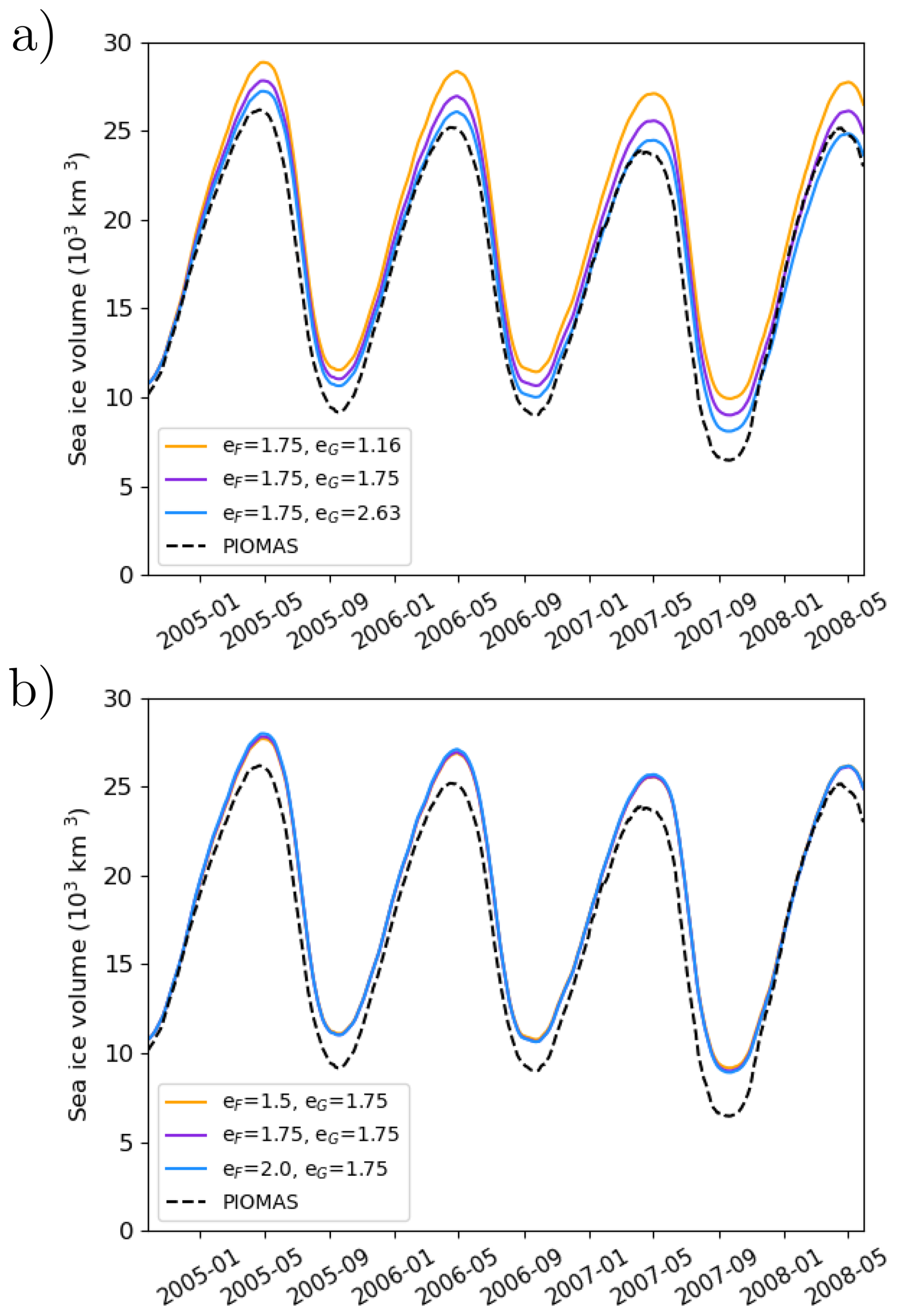
Figure 12 Total simulated daily mean sea ice volume as a function of time for different values of e_F and e_G. As a comparison, the dashed black line shows the sea ice volume simulated by the PIOMAS system.

We interpret this effect of e_G on the sea ice volume to the amount of divergence associated with the flow rule: a smaller e_G leads to a more circular (or less elliptic) plastic potential and therefore normal vectors exhibiting more divergence. This enhanced lead formation with a smaller e_G should be associated with an increase in the sea ice growth. We also argue that the increased divergence associated with the non-normal flow rule (e_G<e_F) also explains the higher LKF density (see Fig. 8) and the reduced mean width (see Fig. 4) of simulated LKFs compared to results with the normal flow rule (e_G=e_F). More divergence decreases the ice strength, concentrates spatially the LKFs and favors their persistence.

To quantify the amount of divergence (${\dot{\mathit{ϵ}}}_{\mathrm{I}}$) compared to shear (${\dot{\mathit{ϵ}}}_{\mathrm{II}}$), we use the angle θ_r as introduced in Eq. (3). Given daily snapshots at 00:00 UTC for the period 1 January to 31 May 2005, θ_r was calculated at all the ocean grid cells inside the pack ice mask when Δ>Δ_min (i.e., the state of stress is plastic). Figure 13a shows the PDF of θ_r for different e_G (with a fixed e_F). Similarly, Fig. 13b shows the PDF of θ_r for different e_F (with a fixed e_G). e_G has a strong impact on the amount of divergence compared to shear while the impact of e_F is small when keeping e_G fixed. The PDF for a large value of e_G exhibits many pure shear events (i.e. θ_r=0); decreasing e_G augments the events of shear plus divergence (or convergence). For all PDFs, the pure divergence or pure convergence events are rare.

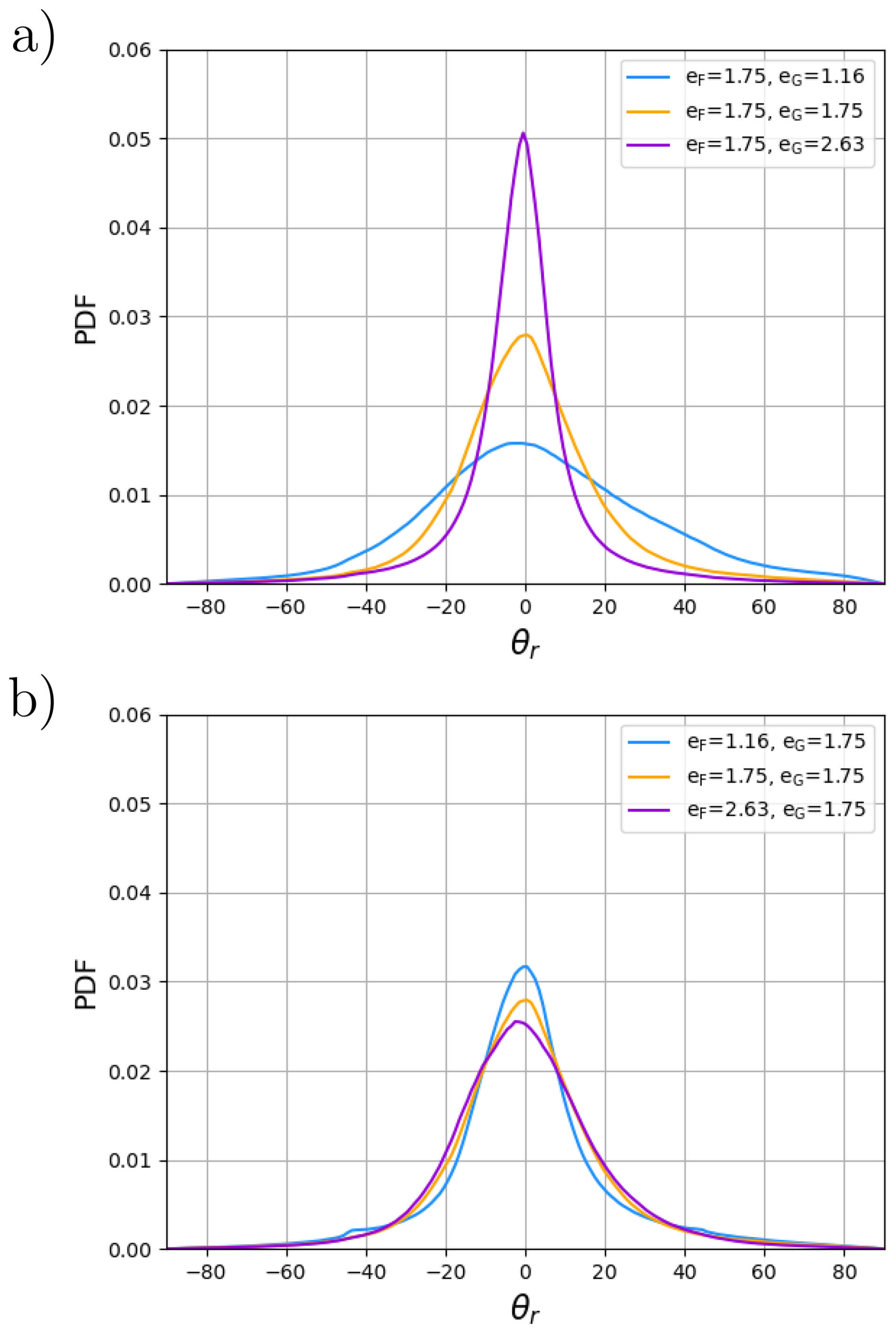
Figure 13 (a) PDF of θ_r for a fixed value of e_F=1.75 and e_G=1.16 (blue), e_G=1.75 (orange), and e_G=2.63 (violet) and e_F=1.5 (blue). (b) PDF of θ_r for a fixed value of e_G=1.75 and e_F=1.16 (blue), e_F=1.75 (orange), and e_F=2.63 (violet). θ_r characterizes the ratio of divergence over shear. The PDFs are calculated from daily snapshots at 00:00 UTC for the period 1 January to 31 May 2005.

Because the sea ice volume time series diverge slightly more with time we only look at the impact of e_F and e_G on the sea ice drift for the period 1 January to 31 May 2005. We choose this time interval because it is close to the beginning of our simulations and during a period (winter-spring) for which rheology has a strong impact on the drift. We interpolated daily averaged velocity components from the U points (corners) to the T points where concentration is calculated. Using these, we calculated the daily spatial averaged sea ice speed. This spatial average was computed for all the grid cells with a concentration larger than 0.15 inside the pack ice mask. Monthly mean values of the daily spatial averaged sea ice speed were then calculated. The results are shown in Fig. 14. Changing the size of the yield curve (i.e., e_F) has a bigger impact on the drift speed than changing the plastic potential (i.e., e_G). In fact, compared to the normal flow rule (e_G=e_F, solid lines), setting e_G<e_F (dashed lines) as proposed by Ringeisen et al. (2021) has a very small impact on the monthly averaged drift speed.

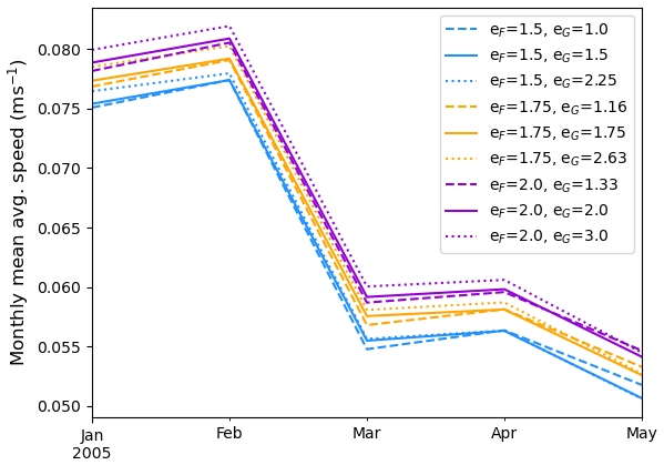
Figure 14 Monthly mean of daily averaged sea ice speed for the period 1 January to 31 May 2005 calculated over the pack ice mask region. The daily averaged sea ice speed is calculated where the daily averaged concentration is larger than 0.15.

Even though the non-normal flow rule does not remedy the problem of too large intersection angles, defining the flow rule independently from the yield curve offers clear advantages. Studies have shown the impact of modifying $e=e_{\mathrm{F}}=e_{\mathrm{G}}$ (i.e., a normal flow rule) on the simulation of ice arches (Dumont et al., 2009) and landfast ice (Lemieux et al., 2016). But clearly, decreasing e to enhance simulated landfast ice in coastal area also impacts the pack ice deformations and the sea ice production in leads. Similarly, modifying e to optimize simulated deformations (Bouchat and Tremblay, 2017) also changes the model ability to simulate landfast ice and ice arches. Our results demonstrate that e_F and e_G could be used to optimize the representation of different physical processes. Modifying the yield curve by changing e_F impacts simulated landfast ice (and ice arches) and to a certain extent the drift of pack ice while modifying the flow rule by changing e_G affects the deformations (and their spatial scaling properties) and indirectly sea ice production in leads.

7 Concluding remarks

We implemented a non-normal flow rule in the CICE sea ice model through the plastic potential approach of Ringeisen et al. (2021). With this formulation, post-failure deformations are normal to a plastic potential curve which is defined independently from the yield curve. This is a very useful capability as it allows to independently optimize critical stresses (i.e. the yield curve) with the parameter e_F and the post-failure deformations with the parameter e_G.

We investigated the impact of a non-normal flow rule in pan-Arctic simulations. Compared to the standard VP rheology (i.e., $e=e_{\mathrm{G}}=e_{\mathrm{F}}$), the non-normal flow rule with e_G<e_F leads to a more active sea ice cover with narrower LKFs and a higher LKF density. As more leads are simulated with a smaller e_G, there is more sea ice formation which notably impacts the sea ice volume. We argue, however, that this impact would be mitigated in simulations using a coupled atmospheric model.

As demonstrated in other studies, we find that the normal flow rule leads to a PDF of intersection angles (for pairs of conjugate LKFs) with a peak at 90°. Using a non-normal flow rule with the elliptical yield curve, as introduced by Ringeisen et al. (2021), does not remedy this problem. Either with e_G<e_F or e_G>e_F, the peak is still at 90°. These results could suggest that LKFs tend to be aligned with the computational grid. This is indeed shown by PDFs of the angle with the grid.

From VP experiments with a normal flow rule, Hutter and Losch (2020) binned all LKFs in 200 × 200 km boxes, computed the orientation distribution, and visually compared its mode(s) with the grid orientation. They could not find a distinct Arctic wide correlation between the modes and the orientation of the grid axes. It is possible that this apparent contradiction with our results is related to the different methods. For instance, the orientation of an LKF contributing to the distribution within a box was defined in Hutter and Losch (2020) as the mean orientation of segments of the LKF laying within the box. In doing so, the orientation of the entire LKF contributed to the analysis. Moreover, Hutter and Losch (2020) included in their analyses all the LKFs, that is conjugate and non-conjugate ones as well as newly formed and old LKFs. For the SIREx project, Hutter et al. (2022) made the qualitative argument that the peak of the PDF at 90° is not caused by LKFs aligned with the grid as models with an unstructured grid also lead to a peak at 90°.

In our quantitative analysis, we only consider newly formed pairs of conjugate LKFs. In doing so, we omit the effect that advection and different types of deformations can have on the orientation of LKFs. We find that conjugate LKFs tend to preferentially orient themselves along the numerical grid axes in a region close to the intersection point. This characteristic can be observed in Figs. 2 and 3 which show the preferred orientation at the intersection points and bended LKFs with varying orientation away from these very same points. Compared to previous studies, the presented analysis therefore offers new insights about the formation of fractures in VP-EVP models.

But why, consistent with theory, smaller fracture angles (by setting e_G<e_F) can be simulated in idealized uni-axial compression experiments (see the supplement of this article and Ringeisen et al., 2021)? We explain as follows this contradiction between realistic pan-Arctic experiments and idealized experiments. We speculate that in the pan-Arctic simulations, a deformation (or fracture) that would be loosely aligned with a grid axis would tend to lock itself to that very same grid axis. This locking mechanism was not observed by Ringeisen et al. (2021) (nor by us, see the supplement of this article) in idealized experiments because simulated fractures exhibit large angles with respect to the grid axes (see for example Fig. 6 in Ringeisen et al., 2021). Understanding and proving the existence of this locking mechanism is beyond the scope of this paper and will be investigated as part of future work. To obtain simulated LKF intersection angles more in line with observations, we argue that not only the rheology needs to be improved but that more advanced numerical methods (i.e., spatial discretization, numerical solver, etc.) should be developed.

Although the non-normal flow rule does not remedy the problem of too wide simulated intersection angles, our results show that e_G could be an additional tuning knob (independent of e_F) for adjusting statistics of LKFs and more generally deformations. On the other hand, the parameter e_F, which defines the shear strength associated with the yield curve, could be used to control the formation of ice arches and more generally the simulated landfast ice area and to a smaller extent to optimize the pack ice drift.

Appendix A: Algorithm for calculating LKF width

The thinning procedure of the LKF detection algorithm identifies a LKF as a series of points each corresponding to the largest total deformation along a perpendicular transect. The LKF points are defined at the T points of the computational grid.

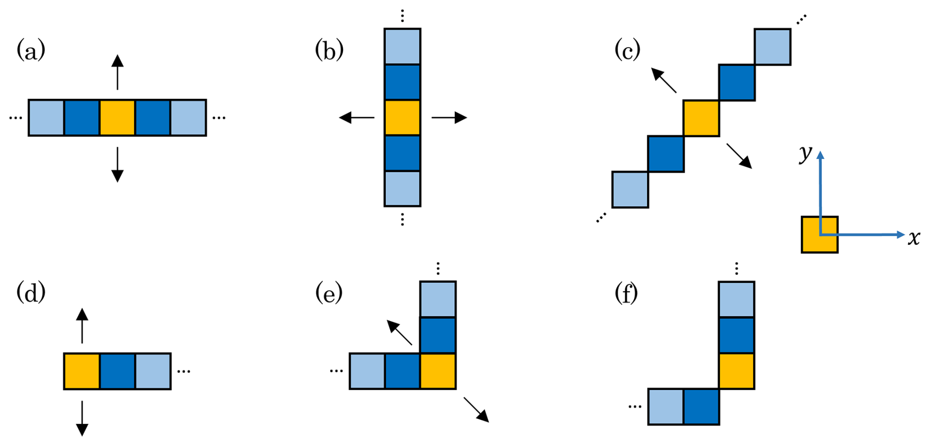
Figure A1 Schematic displaying the search direction algorithm for estimating LKF width for different LKF shapes and orientations. For a given case, the width is calculated from the orange cell. The dark blue cells are used to determine the local direction of the LKF; Light blue cells are not involved. Given a vector locally aligned with the LKF, the search directions (black arrows) are defined at 90° from this vector. There is a case similar to (c) (i.e. at 90°) that is not shown. There are also similar cases to (d) and (e) that are not displayed. The width is not calculated for case (f) (same idea for similar cases) because the search directions are ambiguous. A local x and y coordinate system (shown on the right) is defined for each detected LKF cell and is used by the search direction algorithm. The coordinate i varies along the x axis while j varies along the y axis.

The algorithm for calculating the LKF width is applied for all the N cells (with indices n=0 to $n=N-\mathrm{1}$) of a detected LKF. First, the algorithm determines search directions. This is illustrated in Fig. A1. For a certain cell (in orange) along the LKF, the algorithm calculates the local slope of the LKF with respect to the x axis in order to define a unit vector aligned with the LKF (pointing in the direction of increasing n). Given the coordinates i,j for the orange cell, the x axis is aligned locally with the model grid (i.e., constant j). The dark blue cells in Fig. A1 are the ones used to determine the slope and the unit vector aligned with the LKF. Away from the start and end points of the LKF (panels a, b, c, e and f), two dark blues cells are used and the slope is obtained from a central finite difference. However, at the start point, the orange and dark blue cells are used to calculate the slope from a one-sided finite difference in order to obtain the unit vector aligned with the LKF (panel d). Similar approaches are used for the end point and for diagonal LKFs (not shown).

Two other unit vectors are then defined at 90° from the unit vector aligned with the LKF. These two vectors define the search direction for calculating the LKF width. Note that some points of a detected LKF can lead to ambiguous search directions. An example of this is in panel (f) of Fig. A1. For these points, the width is not calculated and is not used to calculate metrics such as the mean width of LKFs.

The width calculation algorithm calculates the number of grid cells (or pixels) required in both perpendicular search directions for reducing the total deformation below $\mathit{\alpha }{\dot{\mathit{ϵ}}}_{\mathrm{tot}}(i,j)$ where $\mathrm{0}<\mathit{\alpha }<\mathrm{1}$. The parameter α is set to 0.5 in this study. The width of the LKF at a certain point is then the sum of the two half-widths associated with the two search directions. This procedure is illustrated in Fig. A2.

Note that for each search direction, ${\dot{\mathit{ϵ}}}_{\mathrm{tot}}$ is compared to $\mathit{\alpha }{\dot{\mathit{ϵ}}}_{\mathrm{tot}}(i,j)$ up to a maximum number of grid cells defined by c_max. Hence, for the example in Fig. A2, if ${\dot{\mathit{ϵ}}}_{\mathrm{tot}}(i+c_{\max },j)>\mathit{\alpha }{\dot{\mathit{ϵ}}}_{\mathrm{tot}}(i,j)$, the procedure is stopped and the half-width is set to c_max pixels. The parameter c_max is set to 5 is this study. When the width is measured along an oblique direction (e.g. case (c) in Fig. A1), the half widths are integers multiplied by $\sqrt{\mathrm{2}}$.

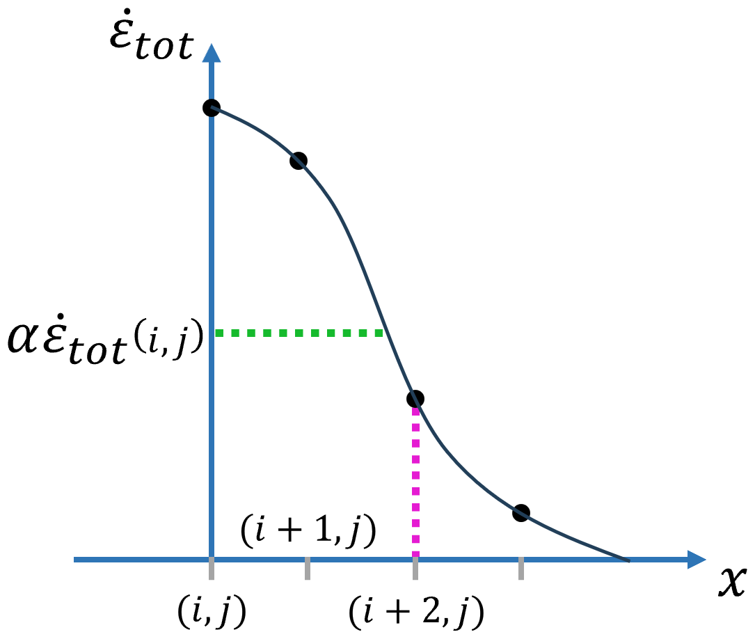
Figure A2 Schematic explaining the method for calculating the half width of a LKF. It is assumed that the LKF is aligned with the y axis. The width is therefore measured along the x axis. This corresponds to case (b) in Fig. A1. The maximum value of the total deformation along the perpendicular transect is ${\dot{\mathit{ϵ}}}_{\mathrm{tot}}(i,j)$. The cell i,j is of course part of this detected LKF. The dotted green line shows the value of $\mathit{\alpha }{\dot{\mathit{ϵ}}}_{\mathrm{tot}}(i,j)$ where in this example α=0.5. The black dots show the value of ${\dot{\mathit{ϵ}}}_{\mathrm{tot}}$ at each grid cell. The half width is defined as the number of pixels required such that ${\dot{\mathit{ϵ}}}_{\mathrm{tot}}<\mathit{\alpha }{\dot{\mathit{ϵ}}}_{\mathrm{tot}}(i,j)$. In this case, the half width is 2 pixels as ${\dot{\mathit{ϵ}}}_{\mathrm{tot}}(i+\mathrm{2},j)<\mathit{\alpha }{\dot{\mathit{ϵ}}}_{\mathrm{tot}}(i,j)$ while ${\dot{\mathit{ϵ}}}_{\mathrm{tot}}(i+\mathrm{1},j)>\mathit{\alpha }{\dot{\mathit{ϵ}}}_{\mathrm{tot}}(i,j)$. The distance between the ${\dot{\mathit{ϵ}}}_{\mathrm{tot}}$ axis and the dotted magenta line is the half width. The profile of total deformation given by the black curve is not used and is simply a visual addition to this schematic. The same procedure is repeated for the left side of this LKF cell.

Appendix B: Algorithm for calculating intersection angles and angles with the grid

The algorithm for calculating intersection angles of pairs of conjugate LKFs first identifies intersecting LKFs. Consider the example in Fig. B1 which shows two intersecting LKFs: LKF1 in blue and LKF2 in yellow. LKF1 has N₁ detected cells (with indices n=0 to $n=N_{\mathrm{1}}-\mathrm{1})$ and LKF2 has N₂ (with indices n=0 to $n=N_{\mathrm{2}}-\mathrm{1})$. The intersection point (the orange cell) has index n=n_i1 for LKF1 and n=n_i2 for LKF2. To determine if LKF1 and LKF2 represent a pair of conjugate LKFs, the algorithm defines local regions for both LKFs for calculating the mean vorticity and for fitting a polynomial of degree 1 (i.e., a line). The region for the polynomial fits are defined by n_min1,n_max1 for LKF1 (same idea for LKF2) with $n_{\min \mathrm{1}}=max(\mathrm{0},n_{i\mathrm{1}}-{\mathrm{\Delta }}_n)$ and $n_{\max \mathrm{1}}=min(n_{i\mathrm{1}}+{\mathrm{\Delta }}_n,N_{\mathrm{1}}-\mathrm{1})$. This local region is represented by the dark blue cells for LKF1 and by the dark yellow cells for LKF2. While Δ_n was set to 10 for the results of this article, it is for simplicity assumed to be equal to four in the example displayed on Fig. B1. Because the top-right cell of LKF2 is the last detected one of this LKF, there are only three LKF cells on the 'right side' of the orange cell for the polynomial fit of LKF2. The polynomial fits are represented by the dashed gray lines.

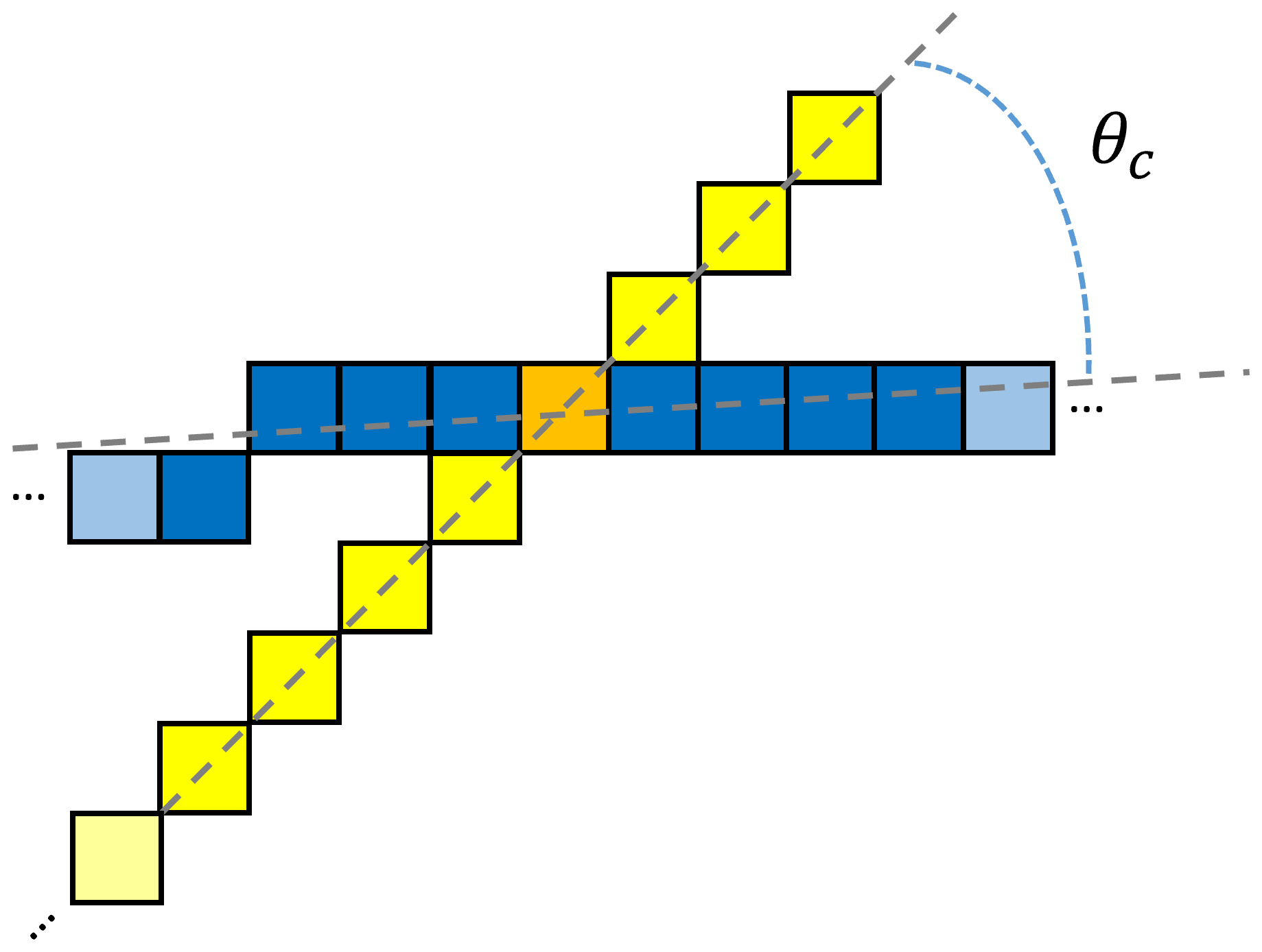
Figure B1 Schematic explaining the algorithm for measuring intersection angles for pairs of conjugate LKFs. The orange cell represents the intersection point between LKF1 (in blue) and LKF2 (in yellow). The dark blues cells are used for the local polynomial fit for LKF1 while the dark yellow ones are used for LKF2. Light blue and light yellow cells are part of the detected LKFs but are not used for the polynomial fits. Δ_n=4 points are used for LKF1 on each side of the intersection points. However, only 3 points are used for LKF2 on one side as the top-right cell is the last point of this LKF. The dashed gray lines are the two polynomial fits. In this example, it is assumed that LKF1 has a positive mean vorticity while LKF2 has a negative mean vorticity (in the local region). The angle θ_c is measured from the polynomial fit for LKF1 to the polynomial fit for LKF2; the angle is acute in this example.

The vorticity is then analyzed for LKF1 in the region of intersection (defined by n_min1,n_max1) and for LKF2 for n_min2 to n_max2. If LKF1 and LKF2 have mean vorticities of opposite sign, they are interpreted as a pair of conjugate LKFs. The angle θ_c is then calculated counterclockwise from the fitted LKF with positive vorticity to the fitted LKF with negative vorticity. In our example, LKF1 (in blue) has a positive mean vorticity while LKF2 (in yellow) has a negative mean vorticity. The angle θ_c is acute in this case.

Given an identified pair of conjugate LKFs as described above, the second part of the algorithm calculates the angles of the conjugate LKFs with a x-y coordinate system defined at the intersection point. The x and y axis of this coordinate system are locally aligned with the computational grid (at the T point). Figure B2 explains how these angles are calculated. The LKF (yellow cells) is LKF2 in the example above for the conjugate angle. Again, the orange cell represents the intersection point between the pair LKF1 and LKF2. The dashed gray line is the polynomial fit for LKF2 in the local region of the intersection point. Given the slope m₂ of the polynomial fit of LKF2, the acute angle θ_x is computed as

$$\begin{array}{}\text{(B1)}& {\mathit{\theta }}_x={\tan }^{-\mathrm{1}}\left|{\displaystyle \frac{m_{\mathrm{2}}-m}{\mathrm{1}+m_{\mathrm{2}}m}}\right|,\end{array}$$

where m=0 is the slope of a line on the x axis.

A similar calculation is done for θ_y. We finally calculate θ_min, the minimum angle, which is simply equal to $min({\mathit{\theta }}_x,{\mathit{\theta }}_y)$. The same process is then repeated for the other conjugate LKF (i.e., LKF1).

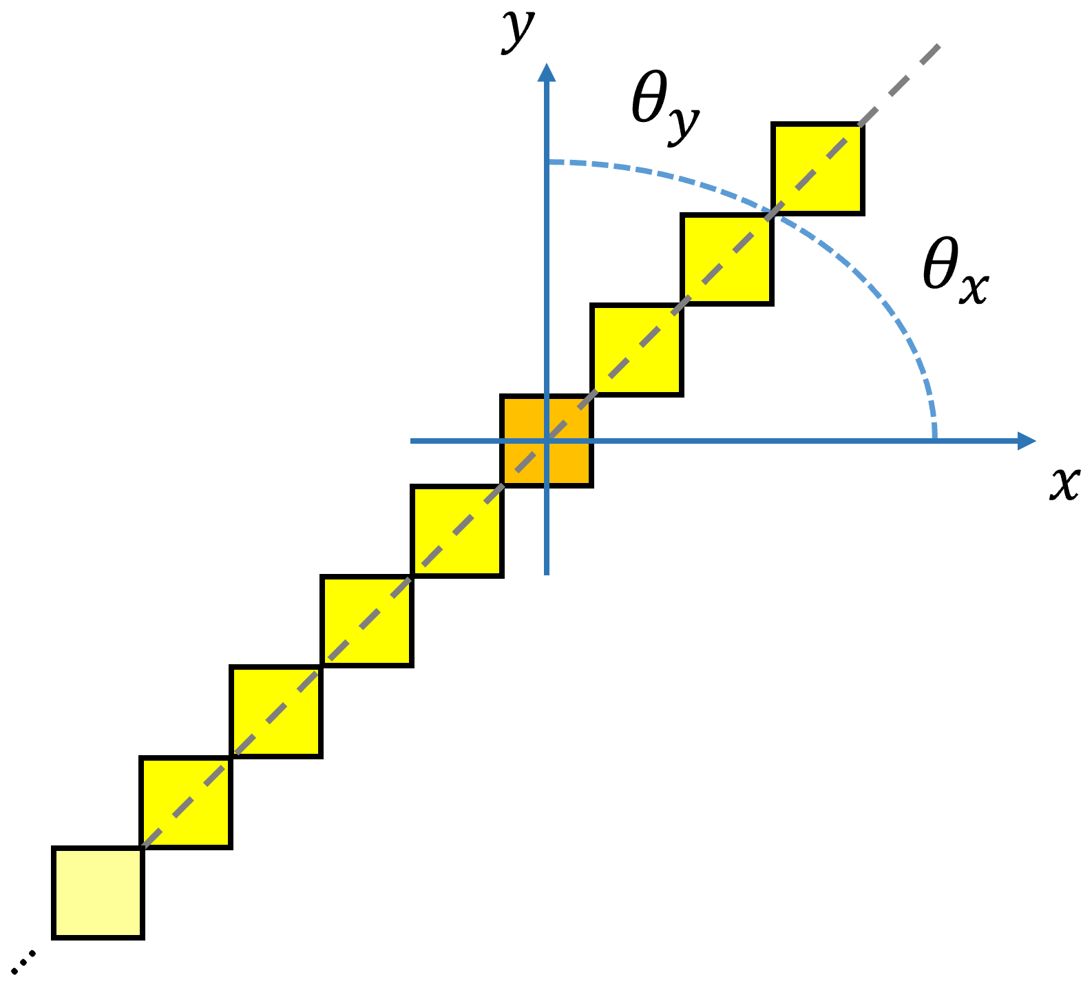
Figure B2 Schematic explaining the algorithm for measuring the angles of pairs of conjugate LKFs with the x axis (θ_x) and with the y axis (θ_y). The orange cell represents the intersection point between the pair LKF1 and LKF2. For clarity, only LKF2 is shown (in yellow). The dashed gray line is the polynomial fit for LKF2 in the local region of the intersection point. The acute angles θ_x and θ_y are measured with respect to a local coordinates system with its origin at the intersection point of the pair of conjugate LKFs. The same process is repeated for the other conjugate LKF (i.e., LKF1).