Four-dimensional variational data assimilation with a sea-ice thickness emulator

Developing operational data assimilation systems for sea-ice models is challenging, especially using a variational approach due to the absence of adjoint models. NeXtSIM, a sea-ice model based on a brittle rheology paradigm, enables high-fidelity simulations of sea-ice dynamics at mesoscale resolution (∼10 km) but lacks an adjoint. By training a neural network as an Arctic-wide emulator for sea-ice thickness based on mesoscale simulations with neXtSIM, we gain access to an adjoint. Building on this emulator and its adjoint, we introduce a four-dimensional variational (4D–Var) data assimilation system to correct the emulator's bias and to better position the marginal ice zone (MIZ). Firstly, we perform twin experiments to demonstrate the capabilities of this 4D–Var system and to evaluate two approximations of the background covariance matrix. These twin experiments demonstrate that the assimilation improves the positioning of the MIZ and enhances the forecast quality, achieving an average reduction in sea-ice thickness root-mean-squared error of 0.8 m compared to the free run. Secondly, we assimilate real CS2SMOS satellite retrievals with this system. While the assimilation of these rather smooth retrievals amplifies the loss of small-scale information in our system, it effectively corrects the forecast bias. The forecasts of our 4D–Var system achieve a similar performance as the operational sea-ice forecasting system neXtSIM-F. These results pave the way to the use of deep learning-based emulators for 4D–Var systems to improve sea-ice modeling.

1 Introduction

Combining observational data with sea-ice models through data assimilation can significantly improve the accuracy of sea-ice forecasts for practical applications such as maritime routing. However, these methods are often computationally expensive. Deep learning offers a promising alternative by providing efficient neural network emulators that act as auto-differentiable surrogates for costly physical models, which frequently lack an adjoint. This enables the implementation of four-dimensional variational data assimilation (4D–Var) systems, potentially enhancing both the accuracy and scalability of sea-ice forecasts.

In this paper, we introduce a 4D–Var system based on the sea-ice thickness (SIT) emulator developed by Durand et al. (2024). This emulator is designed to reproduce the evolution of SIT as modeled by the state-of-the-art sea-ice model neXtSIM (Rampal et al., 2016; Ólason et al., 2022). We first demonstrate the feasibility of employing this emulator and its adjoint within a 4D–Var framework using twin experiments. We then present promising results obtained by assimilating real SIT observations from the CS2SMOS product, which merges CryoSat-2 altimetry with Soil Moisture and Ocean Salinity (SMOS) radiometry (Ricker et al., 2017). Forecasts generated by our system are comparable to those of the operational neXtSIM-F framework (Williams et al., 2021), where -F denotes “Forecast”.

Arctic SIT is strongly influenced by the rheological formulation of sea-ice models. NeXtSIM is built around brittle rheologies (Girard et al., 2011; Dansereau et al., 2016) to better capture small-scale sea-ice processes. At a mesoscale resolution of approximately 10 km, the model successfully reproduces the observed scaling and multifractal properties of sea ice in space and time (Rampal et al., 2019; Bouchat et al., 2022). Two assimilation systems have been developed for neXtSIM to date: an ensemble Kalman filter tested for SIT and concentration (Cheng et al., 2023b), and the operational neXtSIM-F system, which relies on a simple nudging technique (Williams et al., 2021). Here, we present the first application of variational data assimilation methods in neXtSIM, made possible through a data-driven emulator.

We focus on 4D–Var methods, which rely on minimizing a cost function that requires model gradients and adjoints. In the strong-constraint formulation, 4D–Var seeks a model trajectory that best fits the observations over a specified data assimilation window (DAW) (Sasaki, 1970; Talagrand and Courtier, 1987). Gradients are propagated backward in time through the model adjoint during minimization, allowing the initial analysis to integrate observational information from the entire DAW. Adjoint models for sea ice are rarely developed due to numerical instabilities (Kauker et al., 2009; Fenty and Heimbach, 2013). While adjoints of simplified free-drift models exist (Koldunov et al., 2017), they lack realism for full Arctic simulations. Some studies have developed adjoints within coupled ocean–sea ice frameworks using simplified elasto-visco-plastic rheologies (Usui et al., 2016; Toyoda et al., 2015, 2019), but these approaches reduce rheological complexity. Other operational forecasting systems implement alternative assimilation techniques, ranging from ensemble Kalman filters with flow-dependent covariances (Sakov et al., 2012; Kimmritz et al., 2018) to static covariance methods such as optimal interpolation (Wang et al., 2013; Ji et al., 2015) or three-dimensional variational assimilation (Hebert et al., 2015; Toyoda et al., 2015; Lemieux et al., 2015). Initialization by nudging has also been employed (Lindsay and Zhang, 2006; Tietsche et al., 2013).

Recent advances in deep learning for sea-ice modeling span a variety of applications: full emulation of SIT (Durand et al., 2024), probabilities of sea-ice coverage (Andersson et al., 2021), and sea-ice concentration (Liu et al., 2021); as well as more specialized tasks such as model error correction (Finn et al., 2023) and melt-pond emulation (Driscoll et al., 2024). Neural networks have also been integrated into data assimilation workflows, for instance to learn increments for model bias correction (Gregory et al., 2023, 2024a) or to calibrate sea-ice forecasts (Palerme et al., 2024).

In the present work, we leverage the SIT emulator of Durand et al. (2024) for both forward and adjoint modeling within a 4D–Var framework. The principle of emulator-based 4D–Var was first introduced by Hatfield et al. (2021) and demonstrated on Lorenz-63 toy models (Chennault et al., 2021). More recently, it has been applied to numerical weather prediction emulators based on ERA5 reanalyses (Xiao et al., 2023). Our study represents the first 4D–Var data assimilation system designed around an emulator specifically tailored to capture sea-ice dynamics and their adjoint.

We explore two experimental setups. First, we perform twin experiments in which synthetic observations are generated by perturbing neXtSIM outputs. Second, we assimilate real satellite observations from CS2SMOS. The paper is organized as follows: Section 2 introduces the sea-ice model and external forcings; Sect. 3 describes the emulator; Sect. 4 outlines the 4D–Var framework and evaluation metrics; results are presented in Sects. 5 and 6; and Sect. 7 provides a discussion, followed by conclusions in Sect. 8.

2 Physical model simulation and preprocessing of atmospheric forcings

In this section, we begin by introducing the geophysical sea-ice model, neXtSIM, which serves as the ground model for our results. We then present the atmospheric forcings used as additional inputs for the emulator. NeXtSIM is a state-of-the-art sea-ice model (Rampal et al., 2016) built around brittle rheologies (Girard et al., 2011; Dansereau et al., 2016). In the here-used simulations (Boutin et al., 2023), neXtSIM is employed with the brittle Bingham-Maxwell rheology (Ólason et al., 2022) to replicate the observed subgrid-scale behavior of sea ice. Originally run on a Lagrangian triangular mesh, neXtSIM's outputs are projected onto a Eulerian curvilinear grid, forming the basis of our surrogate model (Durand et al., 2024). Additionally, the sea-ice model is coupled with the Nucleus for European Modelling of the Ocean (NEMO) framework's ocean model, OPA (version 3.6, Madec et al., 1998; Rousset et al., 2015). For further information about the numerical model and its setup, we refer to Boutin et al. (2023).

In this study, we predict the sea-ice thickness with a neural network which is trained on simulations spanning from 2009 to 2016. The simulations are run on the regional CREG025 mesh configuration (Talandier and Lique, 2021), a regional subset of the global ORCA025 configuration developed by the Drakkar consortium (Bernard et al., 2006). The simulated area covers the Arctic and parts of the North Atlantic down to 27° N latitude, with a nominal horizontal resolution of 0.25° (≃12 km in the Arctic basin). The data is cropped in lower latitudes and areas in Eastern Europe and America where no sea ice is present, and then coarse-grained by averaging over a 4×4 window, resulting in a final resolution of 128×128 grid-cells. A simulated sea-ice thickness snapshot is displayed in Fig. 1a).

Let $\mathbf{x}\in {\mathbb{R}}^{\mathrm{128}\times \mathrm{128}}$ be the sea-ice thickness. The normalized sea-ice thickness $\stackrel{\mathrm{̃}}{\mathit{x}}$ is then defined by

$$\begin{array}{}\text{(1)}& \stackrel{\mathrm{̃}}{\mathbf{x}}={\displaystyle \frac{\mathbf{x}-{\mathit{\mu }}_{\mathrm{SIT}}}{{\mathit{\sigma }}_{\mathrm{SIT}}}},\end{array}$$

with μ_SIT the globally averaged sea-ice thickness and σ_SIT the global standard deviation, computed over all the coarse-grained grid-cells in the training dataset (2009 to 2016). The subtraction and division are pointwise operations. The normalization of all input fields in the neural network is a common practice to stabilize and speed up the training (Ioffe and Szegedy, 2015). Masking land-covered cells within the original 128×128 grid-cells, N_z=8871 remain unmasked covered by either open water or sea ice. Hence, the data assimilation is performed on the 1-D state vector ${\stackrel{\mathrm{̃}}{\mathit{x}}}^{\mathrm{1}\mathrm{D}}\in {\mathbb{R}}^{N_z}$ which represents the normalized sea-ice thickness on the unmasked grid-cells. We will further drop the 1D superscript for the sake of readability.

Additionally, we also consider the 2 m temperature (T2M), and the atmospheric u- and v-velocities in 10 m height (U10 and V10) from the ERA5 reanalysis dataset (Hersbach et al., 2020). Several atmospheric forcings are added as inputs to the neural network, as sea-ice thickness dynamics are largely driven by the atmosphere (Guemas et al., 2014). In particular, Arctic surface circulation and sea-ice movement are strongly influenced by atmospheric winds (Serreze et al., 1992), while surface temperature fluctuations also play a key role in sea-ice variability (Olonscheck et al., 2019). Interpolated onto the native Eulerian curvilinear grid with nearest neighbors, forcings at time t, t+6h and t+12h are then coarse-grained, normalized and added as predictors to the input of the neural network, as commonly done in sea-ice forecasting (Grigoryev et al., 2022).

3 Surrogate model

In this section, we describe our surrogate model, which has the same structure as the emulator previously developed in Durand et al. (2024), with the only update being that it is trained to account for the positivity of sea-ice thickness during training.

The surrogate model g_θ predicts the full sea-ice thickness ${\stackrel{\mathrm{̃}}{\mathbf{x}}}_{t+\mathrm{\Delta }t}$ with a Δt=12 h lead time. The neural network f_θ with its weights and biases θ is trained to predict the evolution of the SIT after Δt=12 h based on the initial conditions ${\stackrel{\mathrm{̃}}{\mathit{x}}}_t$ and given atmospheric forcings F, $f_{\mathit{\theta }}({\stackrel{\mathrm{̃}}{\mathbf{x}}}_t,{\mathbf{F}}_t)\approx {\stackrel{\mathrm{̃}}{\mathbf{x}}}_{t+\mathrm{\Delta }t}-{\stackrel{\mathrm{̃}}{\mathbf{x}}}_t$. Added to ${\stackrel{\mathrm{̃}}{\mathit{x}}}_t$, this results in the prediction of the full SIT field ${\stackrel{\mathrm{̃}}{\mathbf{x}}}_{t+\mathrm{\Delta }t}$,

$$\begin{array}{}\text{(2a)}& {\displaystyle }{\stackrel{\mathrm{̃}}{\mathbf{x}}}_{t+\mathrm{\Delta }t}& {\displaystyle }=g_{\mathit{\theta }}({\stackrel{\mathrm{̃}}{\mathbf{x}}}_t,{\mathbf{F}}_t)\text{(2b)}& {\displaystyle }& {\displaystyle }=\mathrm{Relu}({\stackrel{\mathrm{̃}}{\mathbf{x}}}_t+f_{\mathit{\theta }}({\stackrel{\mathrm{̃}}{\mathbf{x}}}_t,{\mathbf{F}}_t\left)\right),\end{array}$$

with the point-wise Rectified Linear Unit (Relu) activation function, $\mathrm{Relu}\left(\stackrel{\mathrm{̃}}{\mathbf{x}}\right)=\max ({\mathrm{SIT}}_{\min },\stackrel{\mathrm{̃}}{\mathbf{x}})$, limiting the output to the lower physical bound in the normalized space (SIT_min). Note that f_θ is an intermediate emulator. Firstly, with f_θ, we focus on 12 h tendencies rather than predicting the full state directly, since small changes are harder to capture. The learning process is then split: we first train the emulator to reproduce SIT evolution, and subsequently use transfer learning so that g_θ also respects the positivity constraint thanks to retraining with Relu as the final activation function.

The neural network is trained with a mean-squared error loss between the predicted sea-ice thickness and the targeted sea-ice thickness as simulated by neXtSIM. The main part of the loss function is defined by a pixel-wise mean-squared error (MSE) on all $N_x\times N_y=\mathrm{128}\times \mathrm{128}$ grid-cells, multiplied by the land-sea mask,

$$\begin{array}{}\text{(3)}& \begin{array}{rl}{\mathcal{L}}_{\mathrm{local}}(\mathbf{x},\widehat{\mathbf{x}})& =\mathrm{MSE}(\mathbf{x},\widehat{\mathbf{x}})\\ & ={\displaystyle \frac{\mathrm{1}}{N_x\cdot N_y}}\sum _i^{N_x}\sum _j^{N_y}(x_{i,j}-{\widehat{x}}_{i,j}{)}^{\mathrm{2}}.\end{array}\end{array}$$

Note that, to simplify the equation, we did not include here the land-sea mask, which is applied in the numerical implementation to compute the loss solely on the N_z valid pixels. To address the systematic bias of the surrogate model and to mitigate its influence, which is already accounted for in the MSE loss, we introduce an additional penalty term to the loss function,

$$\begin{array}{}\text{(4)}& {\mathcal{L}}_{\mathrm{global}}(\mathbf{x},\widehat{\mathbf{x}})={\left({\displaystyle \frac{\mathrm{1}}{N_x\cdot N_y}}\sum _i^{N_x}\sum _j^{N_y}(x_{i,j}-{\widehat{x}}_{i,j})\right)}^{\mathrm{2}}.\end{array}$$

Note in particular that the loss in Eq. (4) is squared after averaging, differing from Eq. (3). The total loss is then given by

$$\begin{array}{}\text{(5)}& \mathcal{L}(\mathbf{x},\widehat{\mathbf{x}})={\mathcal{L}}_{\mathrm{local}}(\mathbf{x},\widehat{\mathbf{x}})+\mathit{\lambda }{\mathcal{L}}_{\mathrm{global}}(\mathbf{x},\widehat{\mathbf{x}}),\end{array}$$

with λ weighting the two terms. First, we pre-train the model f_θ using λ=100, as in Durand et al. (2024). Trained until convergence, we select the best model in the validation dataset. Secondly, we fine-tune g_θ to account for the clipping, thanks to the Relu activation function, with a second loss. Here, we select λ=10 as penalty weight, striking a good balance between ℒ_local and ℒ_global which have a different magnitude during second training. Results of the training and inference of the surrogate are presented in Appendix A.

4 Four-dimensional variational data assimilation

In this section, we describe the experimental setup of our 4D–Var, which is based on the surrogate model and its adjoint, as previously discussed in Sect. 3. Note that we are focusing on full 4D–Var rather than incremental 4D–Var.

4.1 4D–Var setup

The forecast model is our data-driven emulator of neXtSIM. ${\stackrel{\mathrm{̃}}{\mathit{y}}}_{\mathrm{k}}$ represents the observation at time k, ${\stackrel{\mathrm{̃}}{\mathit{x}}}^{\mathrm{b}}$ represents the background state, ${\stackrel{\mathrm{̃}}{\mathit{x}}}^{\mathrm{a}}$ represent the analysis and ${\stackrel{\mathrm{̃}}{\mathit{x}}}_{\mathrm{0}}$ the first guess. B is the background error covariance matrix and its specific parameterizations will be described below. To initialize the cycling of the data assimilation, we start with a field as simulated by neXtSIM for 1 January 2016, which is contained in our training dataset and which can be seen as sample from the climatology for the starting day.

For twin experiments, observations are generated directly in the model space, requiring no special preprocessing, as opposed to real observations, as explained in Sect. 6.1. The observation operator ℋ is simply defined as a diagonal matrix H.

In this study, the 4D–Var is cycled across N_cycle cycles. The state at the end of each DAW is used as first guess and background state for the next DA cycle. To evaluate the 4D–Var system, forecasts are run for 45 d after the end of the DAW in the twin experiment case, and for 9 d in the real observations case.

Two types of 4D–Var are considered. 4D–Var-diag, which corresponds to the use of a diagonal matrix as covariance matrix of background errors B (see Sect. 4.2), and 4D–Var-EOF in which the minimization is carried out in the empirical orthogonal function (EOF) space (see Sect. 4.3).

4.2 4D–Var with diagonal B matrix: 4D–Var-diag

The cost function associated to the 4D–Var minimization problem is

$$\begin{array}{}\text{(6a)}& {\displaystyle }\mathcal{J}\left({\stackrel{\mathrm{̃}}{\mathit{x}}}_{\mathrm{0}}\right)& {\displaystyle }={\mathcal{J}}^{\mathrm{b}}+{\mathcal{J}}^{\mathrm{o}}\text{(6b)}& {\displaystyle }& {\displaystyle }={\displaystyle \frac{\mathrm{1}}{\mathrm{2}}}{∥{\stackrel{\mathrm{̃}}{\mathit{x}}}_{\mathrm{0}}-{\stackrel{\mathrm{̃}}{\mathit{x}}}^{\mathrm{b}}∥}_{({\mathit{\lambda }}_{\inf }^{\mathrm{2}}\mathbf{B}{)}^{-\mathrm{1}}}^{\mathrm{2}}+{\displaystyle \frac{\mathrm{1}}{\mathrm{2}}}\sum _{k=\mathrm{1}}^K{∥{\stackrel{\mathrm{̃}}{\mathit{y}}}_k-{\mathbf{H}}_k{\stackrel{\mathrm{̃}}{\mathit{x}}}_k∥}_{{\mathbf{R}}_k^{-\mathrm{1}}}^{\mathrm{2}},\end{array}$$

with

$$\begin{array}{}\text{(7)}& {\stackrel{\mathrm{̃}}{\mathit{x}}}_k={\mathcal{M}}_{\mathrm{0}\mapsto k\cdot \mathrm{\Delta }t}\left({\stackrel{\mathrm{̃}}{\mathit{x}}}_{\mathrm{0}}\right)=\underset{k-\text{times}}{\underbrace{g_{\mathit{\theta }}\circ \mathrm{\dots }\circ g_{\mathit{\theta }}}}\left({\stackrel{\mathrm{̃}}{\mathit{x}}}_{\mathrm{0}}\right),\end{array}$$

and where ${∥\mathbf{x}∥}_{\mathbf{A}}=\sqrt{{\mathbf{x}}^{\top }\mathbf{Ax}}$ is the Mahalanobis norm, and B is defined by $\mathbf{B}={\mathit{\sigma }}_{\mathrm{b}}^{\mathrm{2}}\mathbf{I}$. Through all experiments, ${\mathit{\sigma }}_{\mathrm{b}}^{\mathrm{2}}={\mathrm{0.4}}^{\mathrm{2}}$ (non-dimensional, as $\stackrel{\mathrm{̃}}{\mathit{x}}$ has been normalized). The R_k, defined by ${\mathbf{R}}_k={\mathit{\sigma }}_{\mathrm{obs}}^{\mathrm{2}}\mathbf{I}$ with I the identity matrix, are the observation error covariance matrices, and are all equals. The coefficient λ_inf is a multiplicative inflation term for background errors, which is set to 1 when no inflation is used and is further described in Appendix E. The results of the minimization of the cost function is the analysis ${\mathbf{x}}_{\mathrm{0}}^{\mathrm{a}}$.

4.3 4D–Var projected onto the EOFs basis: 4D–Var-EOF

Empirical orthogonal functions (EOFs) are a set of orthogonal state vectors derived from data, which form a basis of the full state space. Details about the computation and the analysis of the EOFs are given in Appendix B. A reduced strategy to enhance 4D–Var by projecting onto the EOFs has been proposed by Robert et al. (2005) for ocean models. The projection onto the EOFs enables access to cross-covariances and may improve the numerical conditioning of the minimization of 𝒥. The minimization is carried out with respect to the control variable w∈ℝ^m defined by the projection of the vector $\stackrel{\mathrm{̃}}{\mathit{x}}$ onto the matrix ${\mathit{\phi }}_m\in {\mathbb{R}}^{N_z\times m}$:

$$\begin{array}{}\text{(8)}& \stackrel{\mathrm{̃}}{\mathit{x}}=\overline{\mathit{x}}+{\mathit{\phi }}_m\mathit{w},\end{array}$$

with $\overline{\mathbf{x}}$ representing the temporal average sea-ice thickness field over the dataset used to construct the EOFs and m standing for the truncation index corresponding to the number of EOFs which are kept in the definition of the minimization subspace. The goal is to run the 4D–Var minimization in this affine truncated space spanned by the φ_m.

In this subspace, the cost function reads, at cycle n,

$$\begin{array}{}\text{(9)}& \begin{array}{rl}\mathcal{J}\left({\mathit{w}}_{\mathrm{0}}\right)& ={\displaystyle \frac{\mathrm{1}}{\mathrm{2}{\mathit{\lambda }}_{\inf }^{\mathrm{2}}}}{∥{\mathit{w}}_{\mathrm{0}}-{\mathit{w}}_{\mathrm{0}}^{\mathrm{b}}∥}^{\mathrm{2}}+{\displaystyle \frac{\mathrm{1}}{\mathrm{2}}}\sum _{k=\mathrm{1}}^K∥{\stackrel{\mathrm{̃}}{\mathit{y}}}_k\\ & {-{\mathbf{H}}_k{g}_{\mathit{\theta }}^{k\times {\mathrm{N}}_{\mathrm{f}}}(\overline{\mathit{x}}+{\mathit{\phi }}_m{\mathit{w}}_{\mathrm{0}},{\mathbf{F}}_{\mathrm{0}\mapsto k\times {\mathrm{N}}_{\mathrm{f}}})∥}_{{\mathbf{R}}_k^{-\mathrm{1}}}^{\mathrm{2}}.\end{array}\end{array}$$

The details of the 4D–Var cost function computation are presented in Algorithms C1 and C2. The result of this minimization is the control variable at the beginning of the DAW, ${\mathbf{w}}_{\mathrm{0}}^{\mathrm{a}}$. The value of the truncation index is set to m=7000 for all experiments and is further discussed in the Appendix B while further details on the optimization are given in Appendix C.

4.4 Metrics for the evaluation of the experiments

To evaluate the efficiency of the data assimilation scheme, we compute the root-mean-squared error (RMSE) between the predicted state performed by applying the emulator with the analysis as initial state, ${\mathbf{x}}^{\mathrm{f}}\left(t\right)={\mathcal{M}}_{\mathrm{0}\mapsto t\mathrm{\Delta }t}\left({\mathbf{x}}_{\mathrm{0}}^{\mathrm{a}}\right)$, and the truth x_t, which corresponds to the neXtSIM simulation in the twin experiment case, and to CS2SMOS fields in the real observations case, for each cycle n, at the lead time t, and over all unmasked pixels i∈N_z. Inside the DAW (up to 16 d for the twin experiments case and 8 d for the real observations case), this corresponds to an analysis RMSE and afterwards a forecast RMSE. In the case of real observations, the forecast RMSE is computed by comparing our scheme with observations that have not yet been assimilated.

$$\begin{array}{}\text{(10)}& {\mathrm{RMSE}}_n\left(t\right)=\sqrt{{\displaystyle \frac{\mathrm{1}}{N_z}}\sum _{i=\mathrm{1}}^{N_z}\left(x_{i,n}^{\mathrm{f}}\right(t)-x_{i,n}^{\mathrm{t}}(t){)}^{\mathrm{2}}}.\end{array}$$

This RMSE is defined for each cycle of each experiment, and can then be averaged across all cycles to get the mRMSE, which becomes a function depending on the lead time t only.

$$\begin{array}{}\text{(11)}& \mathrm{mRMSE}\left(t\right)={\displaystyle \frac{\mathrm{1}}{N_{\mathrm{cycle}}}}\sum _{n=\mathrm{1}}^{N_{\mathrm{cycle}}}{\mathrm{RMSE}}_n\left(t\right).\end{array}$$

Note that the RMSE and the mRMSE are defined in the physical space, for an easier interpretation. For the evaluation of CS2SMOS assimilation, see Sect. 6, we use two additional metrics, the bias error,

$$\begin{array}{}\text{(12)}& {\mathrm{bias}}_n\left(t\right)={\displaystyle \frac{\mathrm{1}}{N_z}}\sum _{i=\mathrm{1}}^{N_z}{x}_{i,n}^{\mathrm{f}}\left(t\right)-{\displaystyle \frac{\mathrm{1}}{N_z}}\sum _{i=\mathrm{1}}^{N_z}{x}_{i,n}^{\mathrm{t}}\left(t\right),\end{array}$$

and the Ice Integrated Edge Error (IIEE_SIT), as initially introduced by Goessling et al. (2016), but slightly modified by using sea-ice thickness instead of sea-ice concentration as the threshold. Specifically, we define a metric that counts the grid cells where the surrogate model disagrees with CS2SMOS on the presence of sea ice. A grid cell is considered to be covered by sea ice if the thickness exceeds 0.1 m (cf. Durand et al., 2024, B1 for the threshold justification), analogous to the sea-ice concentration threshold of 0.15 defined in Goessling et al. (2016). The IIEE_SIT is expressed as the total area (km²) of disagreement between the observations and the forecast.

5 Twin experiments

In this section, the results from the twin experiments are presented in Sect. 5.2, after the description of the simulated observations in Sect. 5.1.

5.1 Simulated observations from neXtSIM

In the first approach, a twin experiment setup is employed, wherein synthetic observations are generated by adding noise to neXtSIM simulations from 2017 and 2018. Using the observation error variance ${\mathit{\sigma }}_{\mathrm{obs}}^{\mathrm{2}}={\mathrm{0.4}}^{\mathrm{2}}$ (non-dimensional), we define several variants of perturbed observations,

$$\begin{array}{}\text{(13a)}& {\displaystyle }{\stackrel{\mathrm{̃}}{\mathit{x}}}_{\mathrm{t},\mathrm{obs}}^{\mathrm{G}}={\stackrel{\mathrm{̃}}{\mathit{x}}}_{\mathrm{t}}+{\mathit{ϵ}}^{\mathrm{G}},{\mathit{ϵ}}^{\mathrm{G}}\sim \mathcal{N}(\mathrm{0},{\mathit{\sigma }}_{\mathrm{obs}}^{\mathrm{2}}),\text{(13b)}& {\displaystyle }{\stackrel{\mathrm{̃}}{\mathit{x}}}_{\mathrm{t},\mathrm{obs}}^{\mathrm{LN}}={\displaystyle \frac{{\mathit{x}}_{\mathrm{t}}\exp \left({\mathit{ϵ}}^{\mathrm{LN}}\right)-{\mathit{\mu }}_{\mathrm{SIT}}}{{\mathit{\sigma }}_{\mathrm{SIT}}}},{\mathit{ϵ}}^{\mathrm{LN}}\sim \mathcal{N}\left(\mathrm{0},{\mathit{\sigma }}_{\mathrm{obs}}-{\displaystyle \frac{\mathrm{1}}{\mathrm{2}}}{\mathit{\sigma }}_{\mathrm{obs},}^{\mathrm{2}}\right),\text{(13c)}& {\displaystyle }{\stackrel{\mathrm{̃}}{\mathit{x}}}_{\mathrm{t},\mathrm{obs}}^{\mathrm{cond}-\mathrm{clipped}}=\min \left({\stackrel{\mathrm{̃}}{\mathit{x}}}_{\mathrm{t}}\left(\mathrm{1}+{\mathit{ϵ}}^{\mathrm{G}}\right),{\mathrm{SIT}}_{\min }\right).\end{array}$$

with exp the exponential function. The Gaussian observation noise as defined in Eq. (13a), is an idealized case tailored to the common assumptions of 4D–Var, to test an adaptive inflation scheme which will be defined later. Equation (13b) specifies a log-normal distribution for the noise, as more commonly encountered in sea-ice observations from satellites (Landy et al., 2020). Furthermore, a variant to log-normal noise is introduced in Eq. (13c) by adding a fraction of the sea-ice thickness and incorporating clipping, based on SIT_min, the corresponding 0 m thickness in the normalized space. This noise definition is called cond−clipped in the following. This approach ensures that the observations remain confined within the physical bounds of sea ice, unlike Gaussian noise, but similarly to log-normal noise. Examples of the different noises are shown in Fig. 1b–d.

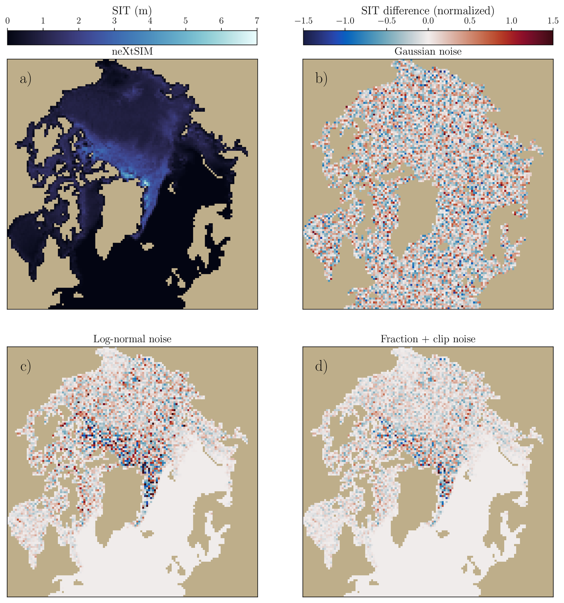
Figure 1 Snapshots of neXtSIM SIT (a) and different type of observations (b) Gaussian noise, (c) log-normal noise (LN) and (d) conditioned noise (cond-clipped). The colorbar for panels (b), (c) and (d) is shared and displayed on the right.

These noise definitions yield different noise magnitudes. The log-normal noise, defined in Eq. (13b), provides a more significant spread, especially for thicker ice. In average, the log-normal noise definition results in a standard deviation of 0.35 m, because of the skewness of the log-normal law, whereas the conditioned noise, defined in Eq. (13c), results in a smaller standard deviation of 0.29 m.

5.2 Results

The length of the DAW is set to N_daw=16 d which corresponds to 32 iterations of the surrogate model. In the twin experiment setup, observations are acquired every 2 d (every N_f=4 iterations). In all twin experiments, we initialize the first data assimilation cycle with a past neXtSIM SIT field from the 1st of January 2016. In this section, the multiplicative inflation coefficient is set to 1. Experiments are conducted throughout years 2017 and 2018, which are after the training dataset (years 2009–2016). To compute averaged results, only the year 2018 is used, i.e. 2017 is used as spin-up. The 4D–Var is run for N_cycle=45 cycles from 1 January 2017 to 21 December 2018.

As shown in Table 1, the choice of noise distribution – whether Gaussian, log-normal, or cond-clipped as defined in Sect. 5.1, influences the efficiency of the assimilation process. However, all experiments remained stable, meaning that there was no divergence in the results. While the assimilation of perfect observations yields the best results, the different noise definitions produce comparable outcomes. Using the cond-clipped perturbations provide the best RMSE among the three different types of perturbations. This could be linked to the lower RMSE of its observations.

Table 1 Comparison of RMSE for different types of simulated observation noise (cf. Sect. 5.1) for the two types of 4D–Var algorithms (with diagonal B matrix and with projection onto the EOFs). Results are presented with the mRMSE computed inside the DAW across 2018. The RMSEs between neXtSIM and the perturbed observations, are outlined in the second column. They correspond to the averaged RMSE between the observations and their associated non-perturbed SIT field.

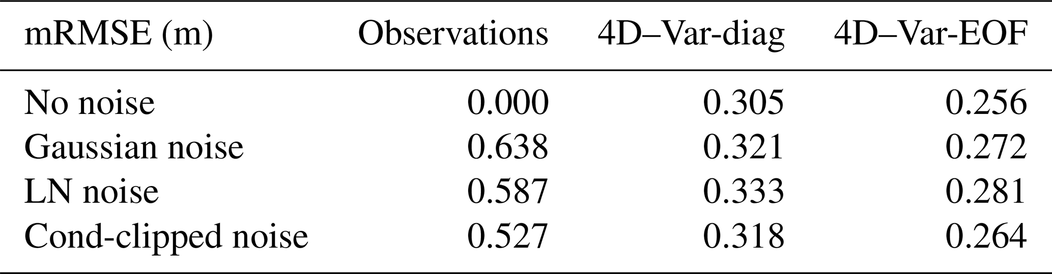
As shown in Table 1, projecting the 4D–Var onto the EOFs yields improvements in all cases, with relative improvements in the range 15 %–17 % for the different types of noise. This improvement can be attributed to the non-diagonal terms in the implied B matrix. This systematic improvement is also observed in Fig. 2 during forecast. When extending the forecast beyond the DAW, the advantage of the 4D–Var-EOF over the 4D–Var-diag remains noticeable but diminishes as the lead time increases. On average, both forecasts show an improvement of 0.8 m over the emulator's free run (initialized on 1 January 2017) across all lead times. Additionally, when comparing the 4D–Var-EOF forecast to the emulator forecast (initialized with perfect conditions at the end of each DAW, red dashed curve), we observe comparable RMSE, showing the stability of the forecast produced by the analysis.

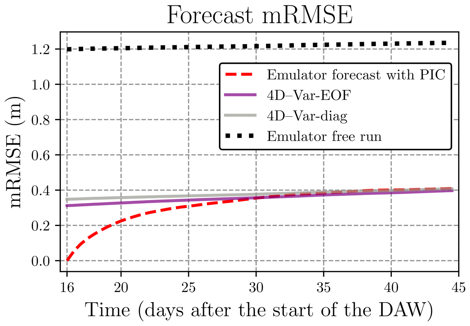
Figure 2 Cycle-averaged mRMSE of ${\stackrel{\mathrm{̃}}{\mathit{x}}}_{\mathrm{f}}$ over 2018 during forecast stage. The dashed red line represents the free run of the emulator started at the end of each DAW (with perfect initial conditions, PIC). The mRMSE of the 4D–Var-EOF forecast is shown in purple, and the 4D–Var-diag forecast is shown using in grey. Cond-clipped noise is used in both cases. The black dotted line corresponds to the emulator free run, initialized on 1 January 2017.

Figure 3 displays fields to illustrate the benefit of data assimilation over a cycle. The first guess field is smoother because of the emulator, whereas the analysis is actually noisier than the truth, because of the observations' noise. The largest negative corrections are applied to the MIZ to correct its position, especially in the Beaufort Sea, Chukchi Sea, and Hudson Bay. In the other places, we observe a positive correction, which is consistent with the negative bias ($\simeq -\mathrm{0.015}\mathrm{m}$) of the surrogate model at the time of the depicted cycle.

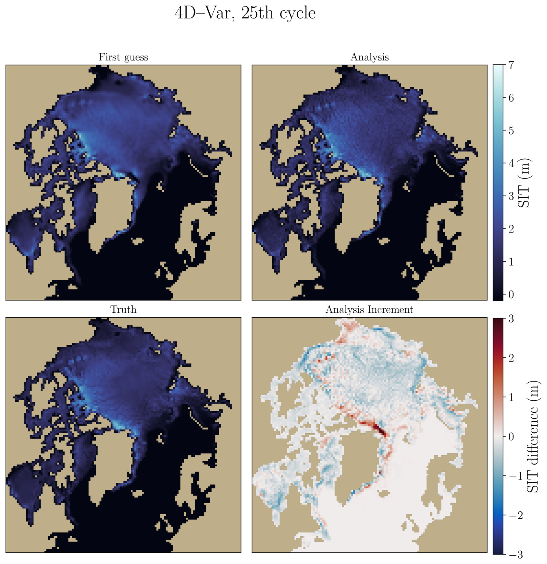
Figure 3 Fields of the SIT at the beginning of the 25th cycle of the DA, corresponding to 5 February 2018, are shown in the 4D–Var-EOF case. The upper left panel represents the first guess, which is the output of the forecast from the previous minimization. The upper right panel corresponds to the analysis of the 25th cycle. For comparison, the associated neXtSIM field, considered as the truth, is displayed in the lower left panel. Note that these three fields share the same colormap and scale. The lower right panel shows the analysis increment, which represents the analysis minus first guess.

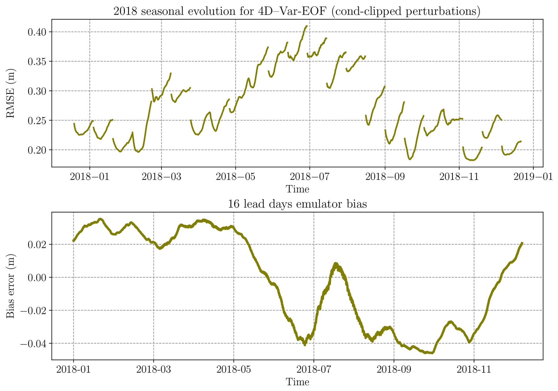
Figure 4 Time evolution of the 4D–Var-EOF analysis RMSE (inside the DAW) in 2018 (upper panel), with cond-clipped simulated noise. Corresponding bias error of the emulator is represented below, as defined in Eq. (A2) with a 16 d lead time, with a new forecast starting every 6 h, at the given time of the x axis.

As seen in Fig. 4, at the start of each cycle, the initial analysis RMSE is generally lower than the first guess RMSE, which corresponds to the end of the previous DAW, indicating that the analysis improves over the first guess, of 2 cm in average across all cycles. In the specific case on late February 2018 (cycle 26), large differences between the truth and the analysis are located near the Canadian Archipelago, leading to a higher RMSE compared to the first-guess RMSE, where such differences do not occur. We hypothesize that, in order to minimize the RMSE throughout the DAW, the 4D–Var removes sea ice in this region. This is consistent with the emulator's positive bias during this period. Overall, the analysis from Fig. 4 (top) reveals a strong seasonality in results, with RMSE peaking in July. The peak aligns with significant changes in sea-ice extent at this period, with an important decrease due to the warmer temperatures in the Arctic. This suggests that 4D–Var possibly struggles more with dynamic shifts. See additional multi-year results in Appendix D. Additionally, the bias error of the emulator (Fig. 4, lower panel), indicative of model error, shows a similar seasonal pattern, transitioning from a positive to negative bias around summer and reverting in December. The key factor affecting assimilation accuracy appears to be not just the amplitude but also the seasonal variation of this bias.

An important factor influencing the quality of the assimilation is the frequency of the observations. We denote the number of observations during one cycle of 16 d (32 model iterations) as N_obs. As shown in Fig. 5, when there are too few observation times per cycle, no improvement is observed in the analysis compared to the forecast at the end of the previous cycle (this is the case for both 2 and 4 observation times per cycle). Once 8 observation times per cycle are reached, this divergence disappears, which is why we choose 8 observation times per cycle in our setup.

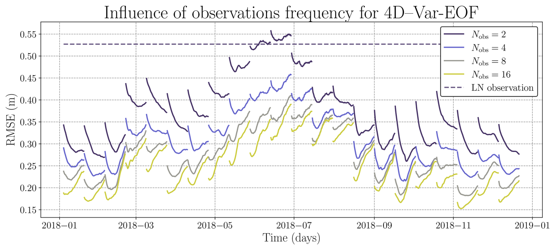
Figure 5 2018 RMSE of 4D–Var-EOF depending on the number of observations in every assimilation cycle in the twin experiment case. Curves indicated the RMSE of the 4D–Var analysis with regard to neXtSIM SIT, with 2 observations per cycle (purple curve), 4 observations per cycle (blue curve), 8 observations per cycle (gray curve) and 16 observations per cycle (green curve). The dashed grey line correspond to the averaged RMSE between log-normal (LN) noise and the truth.

6 CS2SMOS assimilation

In this section, the results from the real observations are presented in Sect. 6.2, after the description of the observations used in Sect. 6.1.

6.1 Real observations: combined Cryosat2-SMOS retrieval

The dataset of CS2SMOS (Ricker et al., 2017) retrievals provides real observations. The retrievals merge observations from CryoSat-2 (Kurtz and Harbeck, 2017), known for its accurate observations of thick and perennial sea ice, and from SMOS (Tian-Kunze et al., 2014), used to infer the thickness of thin ice. Merged weekly to account for the different temporal resolution of CryoSat-2 and SMOS observations, the retrievals are available as daily moving window average. Note that the CS2SMOS is the result of Kriging and has been considerably smoothed in the process, even when compared to a weekly average of neXtSIM, as illustrated in Fig. 7.

CS2SMOS retrievals are only available on grid-cells covered by sea ice, and no information is available on grid-cells with open water. This creates a temporally changing mask, and we assume that grid-cells without information contain no sea ice.

Additionally, the CS2SMOS retrievals come with their own errors and uncertainties (Ricker et al., 2017). Note that Nab et al. (2025) showed that modifying SIT observation uncertainties introduces significant sensitivities during SIT assimilation. Based on the diagnostics of Desroziers et al. (2005), Xie et al. (2018) proposed an empirical formula for the observation error variance ${\mathit{\sigma }}_{\mathrm{obs},\mathrm{CS}\mathrm{2}\mathrm{SMOS}}^{\mathrm{2}}$ as an increasing function of ice thickness h_ice, with the coefficients $\mathrm{0.2},\mathrm{0.02},\mathrm{0.1}$ in m², 3 in m and 1.5 without unit.

$$\begin{array}{}\text{(14)}& {\mathit{\sigma }}_{\mathrm{obs},\mathrm{CS}\mathrm{2}\mathrm{SMOS}}^{\mathrm{2}}=\left\{\begin{array}{ll}\min (\mathrm{0.2},\mathrm{0.02}{e}^{\mathrm{1.8}(h_{\mathrm{ice}}-\mathrm{3})})& \text{if }{h}_{\mathrm{ice}}>\mathrm{3}\mathrm{m},\\ \max (\mathrm{0.02},\mathrm{0.1}{e}^{-\mathrm{1.5}{h}_{\mathrm{ice}}})& \text{otherwise}.\end{array}\right.\end{array}$$

Figure 6 Representation of the function defined in Eq. (14).

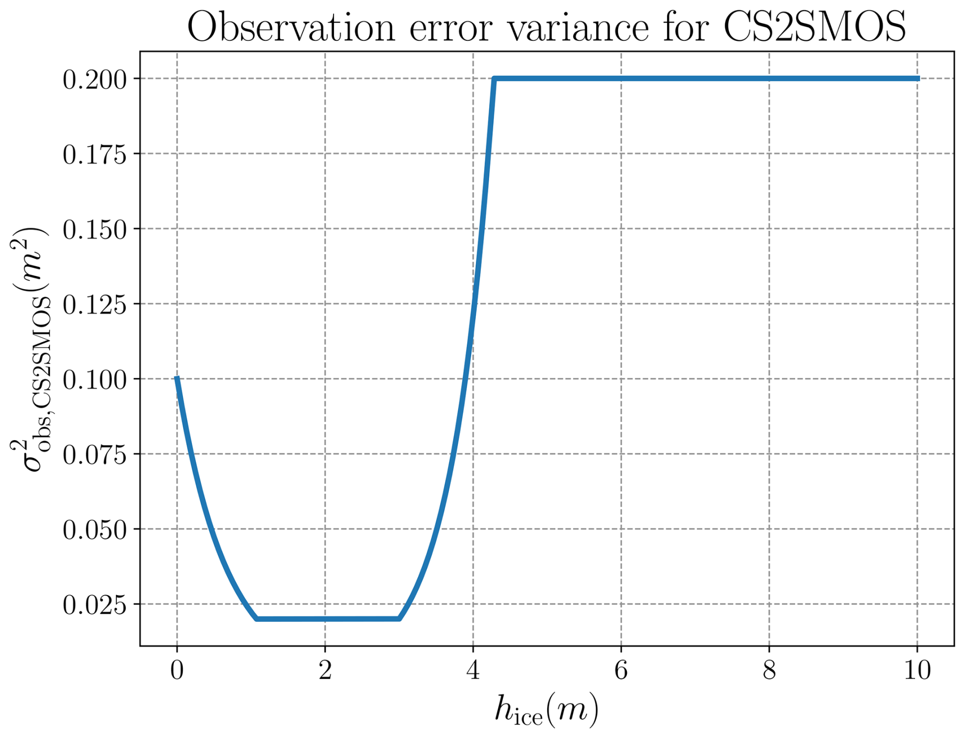
This observation error variance is also used in Cheng et al. (2023a). The graph of the function is displayed in Fig. 6. We will rely on this assessment to introduce observation error statistics for the real observation setup. Note that, unlike the usual approach in data assimilation where the model state is projected onto the observation space using ℋ, we simplify the process by doing the other way around. In a preprocessing step, real observations are interpolated onto the model space, making them retrievals. This is feasible because the observations are at a higher resolution in their native grid, and then coarse-grained by a factor 2. Even in their original resolution, they remain smoother than the forecasts of our surrogate model.

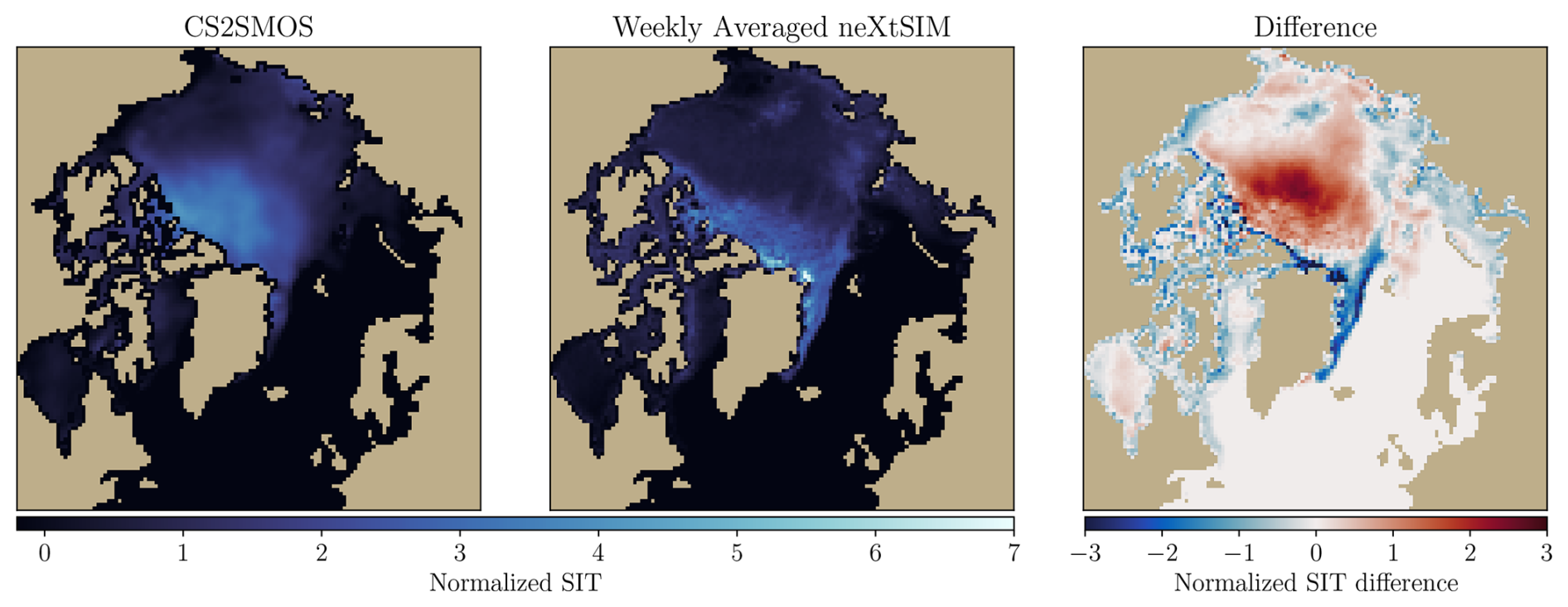
Figure 7 Difference (right) between daily CS2SMOS (left) and neXtSIM SIT (middle). CS2SMOS is interpolated on neXtSIM reduced grid. neXtSIM SIT is averaged over one week in order to mimic CS2SMOS weekly averaging, centered on 4 January 2018.

6.2 Results

In this section, instead of assimilating simulated observations, we assimilate CS2SMOS retrievals daily (every two iterations of the emulator) within an 8 d window for N_cycle=20 cycles. We use the observations for the winter 2020–2021, since there are no CS2SMOS retrievals during summer. We compare the forecasts from the 4D–Var analysis (after the 8 d window) with CS2SMOS observations that have not yet been assimilated, following the standard observation-minus-background (O–B) approach. To initialize the cycling of the data assimilation, we start with the CS2SMOS retrieval from the date of the first assimilation cycle. The observation error variance used is defined in Eq. (14). Only results performed with the 4D–Var-EOF are presented in this section. Note that no multiplicative inflation scheme is used here.

In order to compare the results to a practical forecast benchmark, we use past forecasts from neXtSIM-F (Williams et al., 2021), a forecasting system that consists of a stand-alone version of neXtSIM, forced by the TOPAZ ocean forecast (Sakov et al., 2012) and ECMWF atmospheric forecasts. The past forecasts have been obtained in 2023, corresponding to the version of the forecasting system released in November 2023 (European Union-Copernicus Marine Service, 2020). In neXtSIM-F, the model is nudged to CS2SMOS sea-ice thickness observations weekly. It produces a 9 d forecast, which we systematically use for numerical comparison with our data assimilation scheme, starting the neXtSIM-F forecast at the end of each DAW. Both data assimilation systems are compared directly to CS2SMOS observations for forecasts beyond the DAW.

The 4D–Var analysis is using atmospheric reanalysis F from ERA5 as input for the emulator. For the sake of fairness, for the 9 d forecast that is run beyond the DAW, we use atmospheric forcings from the ECMWF atmospheric model HRES, which provides 10 d forecasts at a 16 km resolution. By contrast, ERA5 is a reanalysis product that assimilates observations, making it unsuitable for an operational forecasting setup where the aim is to predict the future. Therefore, following the approach used in neXtSIM-F, we rely on atmospheric forecasts as forcings of the emulator during the forecast period. These forecasts are interpolated onto the neXtSIM grid and normalized using the same processing method as the ERA5 forcings preparation, replacing them when applying the emulator during forecast.

As seen in Fig. 8, the assimilation of real data into our 4D–Var works and yields RMSEs similar to those of the neXtSIM-F forecast. The free run, initialized with a SIT field from October 2018 (due to the lack of simulation outputs in 2020), produces a stable trajectory but significantly deviates from the CS2SMOS fields. Assimilating real observation yields a substantial decrease in RMSE, of −0.49 m during forecast. Results after the 9 d forecast are compared with the neXtSIM-F 9 d forecast and show similar outcomes. On average, neXtSIM-F has a 0.34 m RMSE while our forecast has a 0.36 m RMSE. Initially, neXtSIM-F exhibits lower RMSEs; however, we see improved results in term of forecast towards the last cycles of the assimilation. Let us note that the RMSE metric penalizes the high level of details of the neXtSIM model more than the emulator that smooths gradually with time.

As seen in the twin experiment results, especially with the Fig. 4, we can infer that our data assimilation system is less efficient during periods of strong dynamic change. This is also shown here, with better results after January, at the end of the refreezing period when comparing the end of each cycle forecast (end of the purple dashed lines) with corresponding neXtSIM-F. Conversely, after the refreezing period, it faces fewer difficulties in predicting the optimal state. Yet, the high initial RMSEs could also be linked to the spin-up of the assimilation.

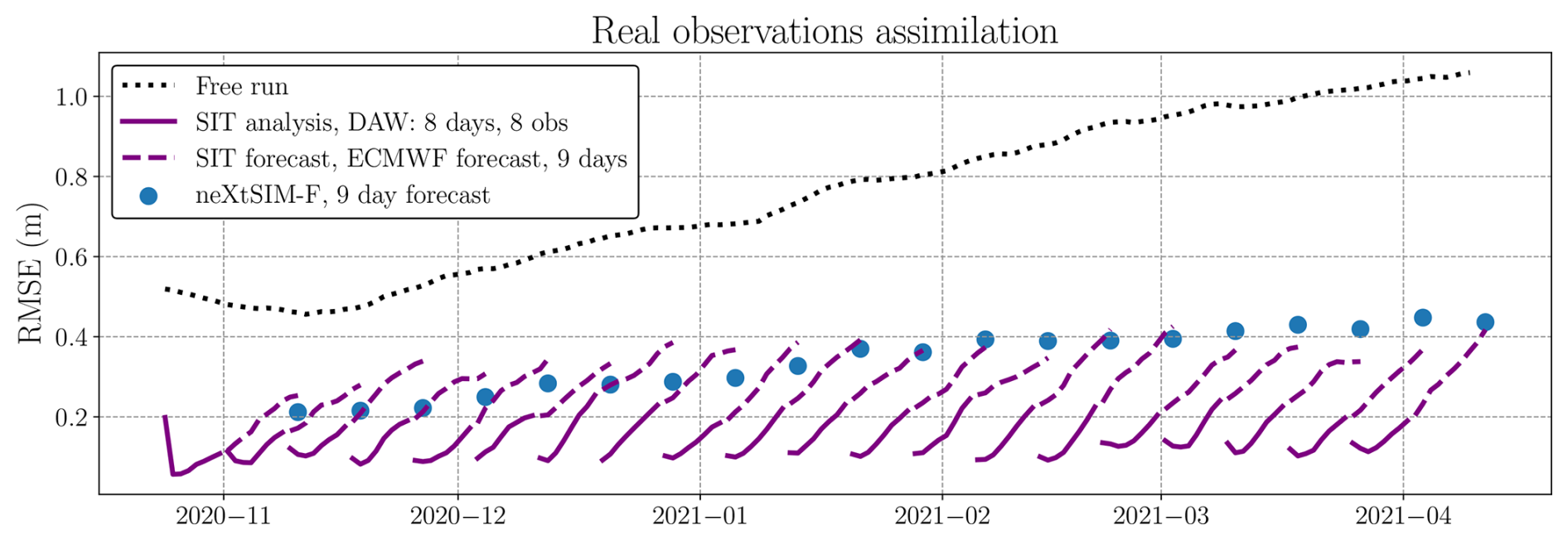
Figure 8 RMSE results for CS2SMOS assimilation across several DAWs throughout the full CS2SMOS observation period in 2020–2021 are shown. The black dotted line represents the free run of the emulator through all cycles, initialized with a SIT field from October 2018. The solid purple line corresponds to the analysis of the 4D–Var over the DAW, while the associated dashed purple lines represent the additional forecasts using ECMWF atmospheric forecasts for 9 d. The RMSE values from neXtSIM-F, corresponding to a 9 d forecast, are displayed as blue dots and should be compared with the end of each corresponding dashed line. All RMSE values are computed with CS2SMOS considered as the truth.

Similarly, to evaluate our assimilation framework, we use the bias error and the IIEE_SIT as defined in Sect. 4.4 in the same data assimilation cycles, see Fig. 9. The absolute value of the bias of the emulator free run is generally reduced, with the exception of December 2020, where the free run bias is smaller than the forecast bias. At the end of the forecast, the assimilation run brings a bias reduction of 6.7 cm compared to the free run. The average bias of the assimilation run compared to CS2SMOS at the end of the forecast is −0.22 cm, while the bias of neXtSIM-F is −1.5 cm. The biases at the beginning of the DAWs are systematically positive and then generally decrease. Since the emulator tends to reduce the amount of sea ice, as indicated by its negative bias, the analysis overestimates sea ice to compensate for this loss. NeXtSIM, on which the emulator is trained, has a different SIT distribution than CS2SMOS, which could explain this phenomenon, as it can be seen with the different order of magnitude of the bias between the emulator initialized with neXtSIM fields in Fig. 4b) (around 0.02 m) and the emulator initialized with CS2SMOS (around 0.1 m). Additionally, the IIEE_SIT serves as a reliable indicator of how accurately the MIZ is positioned. The IIEE of neXtSIM-F is 469 km² and is slightly better than that of the assimilation run 522 km². At the end of each forecast, the assimilation run shows an improvement of 1400 km² in IIEE compared to the free run, highlighting a significant enhancement in MIZ positioning achieved through the 4D–Var-EOF assimilation.

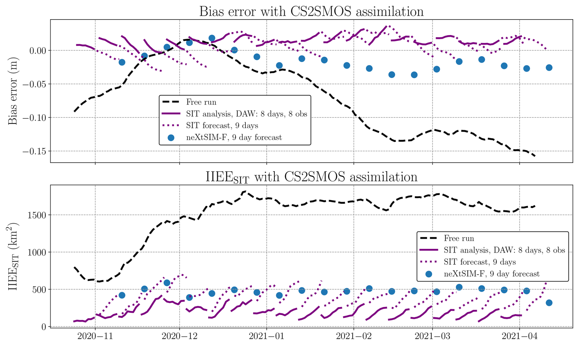
Figure 9 Bias (upper panel) and IIEE_SIT (lower panel) results for CS2SMOS assimilation across several DAWs throughout the full CS2SMOS observation period in 2020–2021 are shown. The black dashed line represents the free run of the emulator through all cycles, initialized with a SIT field from October 2018. The solid purple line corresponds to the analysis of the 4D–Var over the DAW, while the associated dotted purple lines represent the additional forecasts using ECMWF atmospheric forecasts for 9 d. The bias errors and IIEE from neXtSIM-F, corresponding to a 9 d forecast, are displayed as blue dots and should be compared with the end of each corresponding dashed line. All bias errors and IIEE are computed with CS2SMOS considered as the truth.

The data assimilation analysis acts as a bias correction for the emulator. However, it relies on smooth observations, thereby losing the small-scale information available in neXtSIM and neXtSIM-F, as illustrated in Fig. 10. In the twin experiment case, in Fig. 3, we observe that the first guess, corresponding to the end of the previous cycle forecast, appears smoother than the truth. This smoothing is linked to the deterministic nature of the emulator (Durand et al., 2024), as it optimizes its MSE loss by smoothing fine-scale dynamics. While in the twin experiments, the use of observations closely aligned with neXtSIM could help recover some small-scale dynamics, smooth observations result in a complete loss of these finer details. Nevertheless, our data assimilation system effectively acts as a model error correction mechanism.

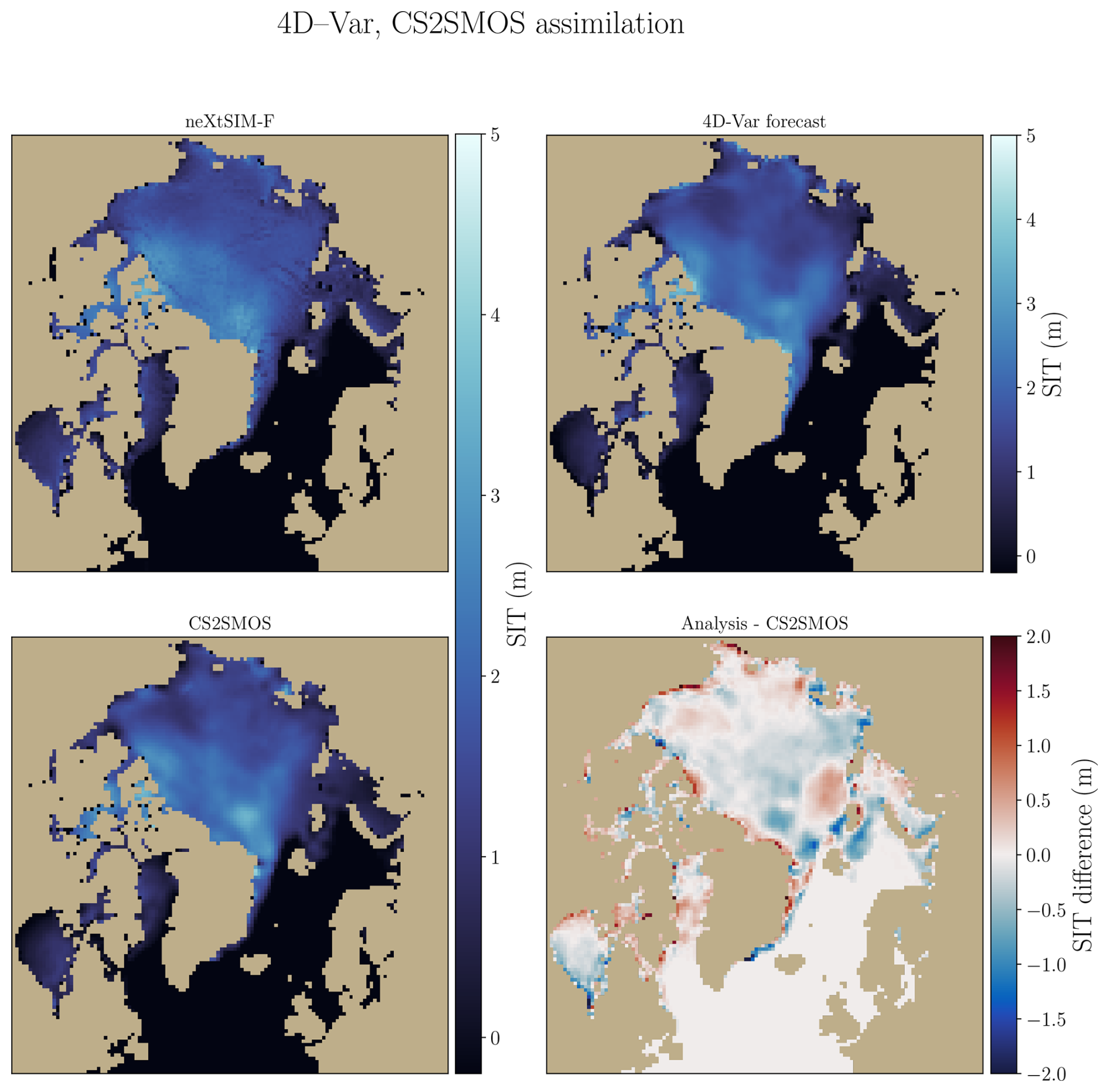
Figure 10 Visualization of the forecast for 26 March 2021 is shown. The upper left panel displays the neXtSIM-F 9 d forecast, while the upper right panel shows the 9 d forecast from the 4D–Var. The lower left panel presents the CS2SMOS observations, and the lower right panel illustrates the difference between the 4D–Var forecast and the CS2SMOS observations.

7 Discussion

We have demonstrated that using an emulator as a forecast model in a 4D–Var framework for sea-ice forecasting is feasible, thanks to its numerical efficiency and auto-differentiability. However, this approach raises several important questions. One key observation is that while replacing the physics-based model with an emulator allows for the benefits of adjoint optimization in a 4D–Var system, the success of the data assimilation is inherently tied to the emulator's accuracy. As illustrated in Fig. 3, the emulator tends to smooth SIT during forecasts extending up to 16 d, a behavior previously noted in Durand et al. (2024).

In the case of real observations, we observe a significant bias correction in the assimilation run. It is worth noting, however, that this study does not consider weak-constraint 4D–Var, which incorporates model error into the cost function minimization. We speculate that improving the emulator's quality – addressing both bias and smoothing issues – would result in more accurate 4D–Var analyses.

An analysis comparing the numerical efficiency of the 4D–Var method between 4D–Var-diag and 4D–Var-EOF is presented. For twin experiments, all computations were executed on a single NVIDIA A100 SXM4 80 GB GPU. On average, over a full data assimilation run of 45 cycles, 4D–Var-EOF takes 155 s per cycle, while 4D–Var-diag takes approximately 229 s per cycle, making 4D–Var-EOF about 32 % faster. Although the gradient computation times differ slightly between the two methods – 1.66 s for 4D–Var-EOF versus 1.36 s for 4D–Var-diag – the forward pass through the DAW is similar, with times of 578 and 552 ms, respectively. The computation of the gradient involves the emulator adjoint evaluation, reshaping the one-dimensional vector of assimilated grid cells into the two-dimensional field required to run the emulator, and computing the cost function term gradients. Interestingly, while individual operations are faster in 4D–Var-diag (as expected due to the absence of projections to and from the EOF basis), the complete cycles are faster with the EOF-based method. In other words, fewer iterations of the L-BFGS optimizer are required on average for 4D–Var-EOF to achieve the analysis at each cycle, indicating better conditioning of the minimizations.

A significant reduction in RMSE (16 %) was achieved by projecting the minimization onto the EOF basis. Although a substantial number of EOFs is retained in the ensemble to preserve information, it is conceivable that computational time could be further reduced by decreasing the number of EOFs. However, the forward pass of the emulator and the computation of its adjoint are inherently performed in the physical space (128×128 grid cells). Consequently, computational time savings from reducing the number of EOFs may not be substantial. On the other hand, this reduction might lead to a loss of small-scale information, as observed in Fig. B2, where the RMSE increases as the truncation index decreases, down to a certain threshold.

We introduce in Appendix E an inflation scheme to tune the background cost function term. Two versions are evaluated: the more commonly used constant inflation and an adaptive scheme based on the ${\mathit{\chi }}_p^{\mathrm{2}}$ (with p degrees of freedom) diagnostic (Michel, 2014). Adaptive background error inflation can be easily implemented in twin experiment scenarios under Gaussian noise simulation. We observe a modest improvement in the time-averaged RMSE, with most of the gains occurring at the beginning of each assimilation window. Interestingly, in both cases, we have to deflate the B-matrix for an optimal analysis RMSE (around 0.5 to 0.6, with a seasonal dependency).

A major factor affecting the RMSE is the frequency of the observations. While most of the results above focus on a fixed number of observations per cycle, additional experiments with varying frequencies in a twin experiment setup (Fig. 5) show substantial RMSE improvement when increasing the observation frequency. However, current satellite data either provide temporally sparse observations with dense along-track but sparse cross-track coverage (e.g., CryoSat-2), or smooth, time-averaged full coverage products that introduce inherent correlations between observation errors (e.g., CS2SMOS). It is important to note that our comparison with neXtSIM-F occurs 9 d after the last batch of assimilated observations, thus falling outside the DAW. Yet, for real observations, no SIT retrieval dataset currently provides daily, non-smoothed, and non-time-correlated SIT measurements for validation. Promisingly, ongoing work is exploring ML-based approaches to derive complete daily sea-ice freeboard fields from satellite altimetry at fine spatial resolution (5 km), by modeling the spatio-temporal covariance of daily fields rather than relying solely on temporal averaging (Gregory et al., 2024b; Chen et al., 2024).

It should be noted that neXtSIM, as well as neXtSIM-F, exhibits more small-scale features than our emulator, which tends to smooth the fields. By assimilating CS2SMOS observations, we lose small-scale information. However, since the observations themselves are extremely smooth, the comparison is not entirely fair to neXtSIM-F, which provides more small-scale dynamics and thus suffers from double penalty effects. Implementing a stochastic emulator (Finn et al., 2024a, b) could yield more physically consistent results by conserving spectral energy. This approach may enhance model performance within the 4D–Var minimization framework, although it raises questions about the reliability of the associated gradients and the increased computation time. Newer satellites will hopefully provide higher-resolution and more accurate data, but the current trade-off between resolution (altimeters) and coverage (passive microwaves) will likely remain in the foreseeable future. Another option is to apply super-resolution algorithms to enhance local-scale dynamics in the data assimilation system (Barthélémy et al., 2022). Exploring these possibilities could significantly improve the efficacy of data assimilation with emulators for sea-ice modeling. An important aspect to monitor is the evolution of the cost function during minimization, as well as its associated gradient. More details are provided in Appendix C. As shown in Fig. C2, there is more than an order of magnitude difference in the gradient norm during minimization within a single cycle. It is worth noting that the only stopping criterion consistently achieved is related to the tolerance of the cost function, where its decrease becomes smaller than a given value. Occasionally, a second criterion related to the gradient norm may also be considered, which requires that the maximal gradient value across the field fall below another specified threshold. However, this gradient criterion is never met in our case. As shown in Fig. C2, some grid cells, often located in the MIZ, retain a non-negligible gradient norm. Nevertheless, at each cycle, the cost function attains a stable minimum (Fig. C1), indicating that the L-BFGS optimization worked correctly.

An important point to discuss is the realism of the emulator's adjoint. In deep learning, the large number of degrees of freedom often results in noisier gradients (Sitzmann et al., 2020). In the 4D–Var framework, this issue is mitigated by the background term, which regularizes the emulator's potentially noisy gradient. This noise is evident in the analysis (Figs. 3 and C2), particularly near the MIZ. While a dedicated training procedure for the emulator could potentially improve this aspect, it does not appear to hinder the current 4D–Var setup. In fact, the successful results achieved with this system indirectly validate the adjoint of both the emulator and the cost function. Furthermore, correctness checks for both adjoints are provided in Appendix C4.

Since the emulator provides fast forecasts of SIT dynamics, and given the efficiency of the data assimilation, we can investigate the possibility of running ensemble data assimilation (EDA) (Raynaud et al., 2008; Isaksen et al., 2010) by executing an ensemble of 4D–Var runs with perturbations applied to the observations and the background term. This ensemble can be used to generate trajectories, but also to improve the flow dependency of the background covariances in EOF space. Interestingly, this approach also enables comparisons with other data assimilation methods using the same emulator, such as the ensemble Kalman filter. This would allow for a more straightforward comparison with current state-of-the-art sea-ice data assimilation methods. However, the ability of our deterministic surrogate model to generate a state ensemble in this context requires further discussion.

8 Conclusions

In this paper, we introduce the first 4D–Var system based on a surrogate model trained to fully emulate the evolution of sea-ice thickness. This work represents a preliminary step toward the use of fully emulated models in data assimilation. Through twin experiments, we first demonstrate the ability of the surrogate model to leverage its automatic gradients in a 4D–Var minimization. The 4D–Var system can be efficiently implemented using EOFs extracted from the model climatology. Assimilation in EOF space improves performance compared to using a diagonal background covariance, while inflation techniques provide only marginal additional benefits. In the second part of the study, we investigate the assimilation of real observations with the 4D–Var system. Assimilating real data improves the positioning of the MIZ, acting effectively as a bias correction. This highlights the potential need for weak-constraint 4D–Var to explicitly address such biases. It also opens opportunities to train a dedicated bias-correction model or to refine the emulator using analysis increments. With limited resources – emulating only sea-ice thickness and assimilating CS2SMOS observations – the developed 4D–Var system performs comparably to the operational neXtSIM-F system. Moreover, the emulator-based 4D–Var system is significantly more computationally efficient than ensemble Kalman filter systems relying on geophysical models. Although these results are derived from a coarse-grained emulator trained on the available neXtSIM dataset, no major obstacles are anticipated when increasing the resolution of both the surrogate model and the assimilated observations. The computational cost of this approach remains well within the standards of current sea-ice data assimilation systems. Overall, these results are promising and demonstrate the potential of using model emulators in data assimilation, particularly when applying classical methods in real-world forecasting contexts. Future work could also explore the impact of assimilating multiple variables, such as SIT and sea-ice concentration, within the emulator framework.

Appendix A: Surrogate modeling

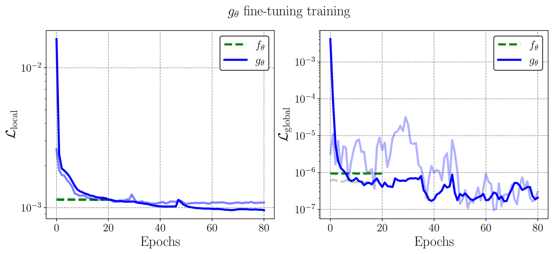
Figure A1 Left: Training and validation losses of the surrogate model. Right: Training and validation global losses of the surrogate models. Light blue and light green lines in transparency indicate the validation losses. The green dashed line indicates the experiment where the weights of f_θ are frozen and a linear activation function is applied after the renormalization process. Blue line corresponds to the training of g_θ. The weights of f_θ are retrained with the new learning objective, with λ=10.

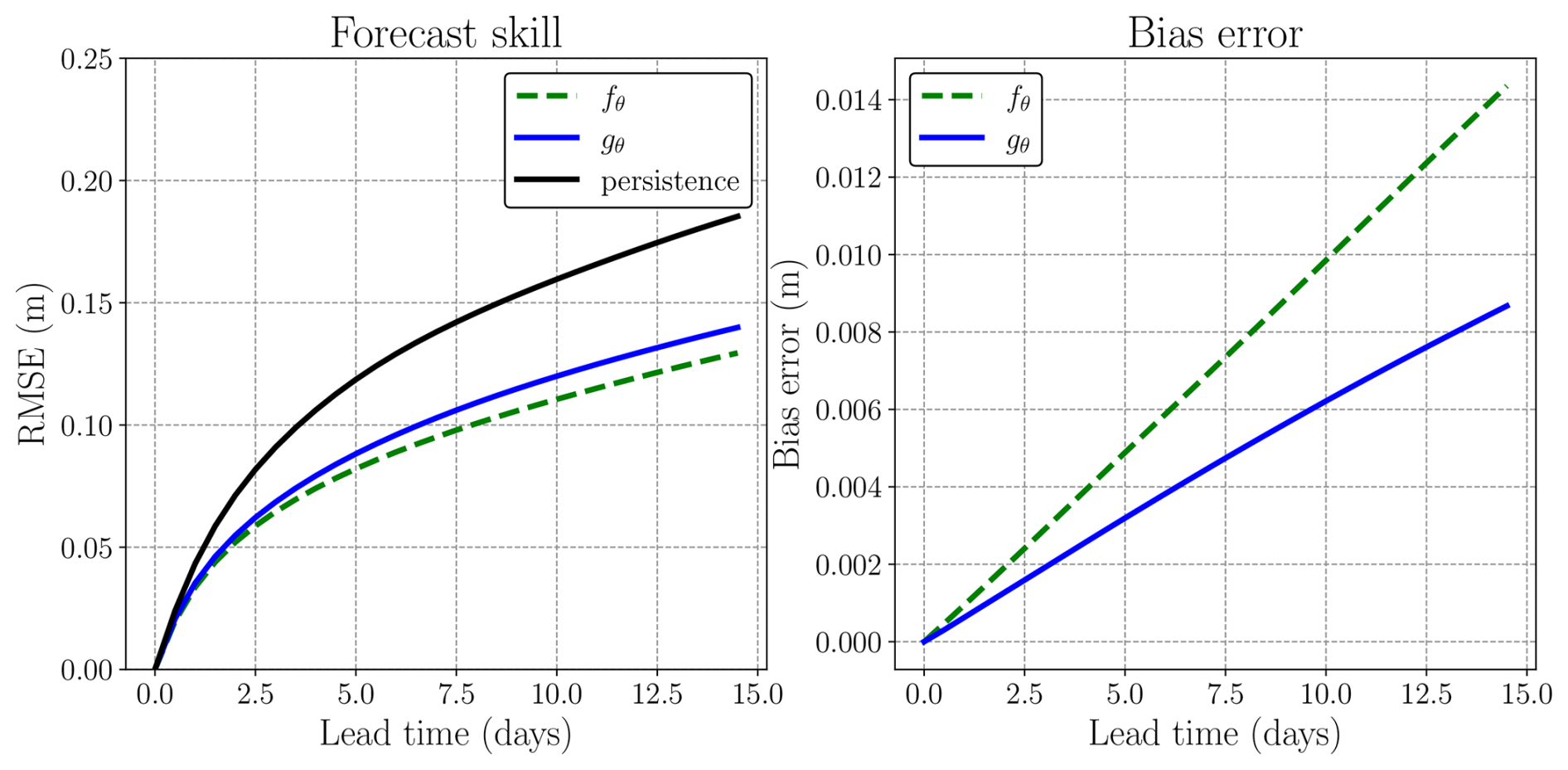
Figure A2 Left: Forecast skill (RMSE) of the surrogate model. Right: Bias errors of the surrogate models. The green dashed line indicates the results for f_θ. Blue line corresponds to the training of g_θ. The weights of f_θ are retrained with the new learning objective, with λ=10.

In this section, we present the forecast ability of the emulator. The root-mean-squared error (RMSE) between the prediction x^f and the simulation x^t is computed over all pixels (i, j) of the field of size (N_x,N_y), for each sample n of the validation set containing N_s=1470 trajectories, initialized at time t_n,

$$\begin{array}{}\text{(A1)}& \mathrm{RMSE}\left(k\right)={\displaystyle \frac{\mathrm{1}}{N_{\mathrm{s}}}}\sum _{n=\mathrm{1}}^{N_{\mathrm{s}}}\sqrt{{\displaystyle \frac{\mathrm{1}}{N_x\cdot N_y}}\sum _{i,j}^{N_x,N_y}{\left(x_{i,j}^{\mathrm{f}}(t_n+k\mathrm{\Delta }t)-x_{i,j}^{\mathrm{t}}(t_n+k\mathrm{\Delta }t)\right)}^{\mathrm{2}}}.\end{array}$$

In order to quantify systematic errors of the surrogate model, we compute its mean error (bias). This metric tells about the ability of the neural network to correctly estimate the total amount of sea ice in the full domain,

$$\begin{array}{}\text{(A2)}& \begin{array}{rl}\mathrm{bias}\left(k\right)& ={\displaystyle \frac{\mathrm{1}}{N_{\mathrm{s}}}}\sum _{n=\mathrm{1}}^{N_{\mathrm{s}}}{\displaystyle \frac{\mathrm{1}}{N_x\cdot N_y}}\\ & \cdot \sum _{i,j}^{N_x,N_y}\left(x_{i,j}^{\mathrm{f}}(t_n+k\mathrm{\Delta }t)-x_{i,j}^{\mathrm{t}}(t_n+k\mathrm{\Delta }t)\right).\end{array}\end{array}$$

The code structure of the surrogate model g_θ is presented in Algorithm A1. Let us note that f_θ maps ${\stackrel{\mathrm{̃}}{\mathit{x}}}_t$ to ${\stackrel{\mathrm{̃}}{\mathbf{y}}}_{t+\mathrm{\Delta }t}={\stackrel{\mathrm{̃}}{\mathit{x}}}_{t+\mathrm{\Delta }t}-{\stackrel{\mathrm{̃}}{\mathit{x}}}_t$ which corresponds to the normalized difference in sea-ice thickness over 12 h. The normalization is defined as in Eq. (1) with μ_out and σ_out the associated global mean and standard deviation of ${\mathbf{y}}_{t+\mathrm{\Delta }t}={\mathbf{x}}_{t+\mathrm{\Delta }t}-{\mathbf{x}}_t$, computed over the training dataset.

Algorithm A1 Full-state surrogate model g_θ mapping from ${\stackrel{\mathrm{̃}}{\mathbf{x}}}_t$ to ${\stackrel{\mathrm{̃}}{\mathbf{x}}}_{t+\mathrm{\Delta }t}$, using the previously trained f_θ. This algorithm describe exactly how the state ${\stackrel{\mathrm{̃}}{\mathit{x}}}_{t+\mathrm{\Delta }t}$ is obtained by the application of the fine-tuned f_θ neural network as defined in Eq. (2b).

Require:

$f_{\mathit{\theta }}({\stackrel{\mathrm{̃}}{\mathbf{x}}}_t,\mathbf{F},\mathit{\theta })$, ${\stackrel{\mathrm{̃}}{\mathbf{x}}}_t$, F, and normalization values (μ_SIT, σ_SIT, μ_out, σ_out)

${\stackrel{\mathrm{̃}}{\mathbf{y}}}_{t+\mathrm{\Delta }t}\leftarrow f_{\mathit{\theta }}({\stackrel{\mathrm{̃}}{\mathbf{x}}}_t,\mathbf{F},\mathit{\theta })$

${\mathbf{y}}_{t+\mathrm{\Delta }t}\leftarrow {\mathit{\sigma }}_{\mathrm{out}}{\stackrel{\mathrm{̃}}{\mathbf{y}}}_{t+\mathrm{\Delta }t}+{\mathit{\mu }}_{\mathrm{out}}$

${\mathbf{x}}_t\leftarrow {\mathit{\sigma }}_{\mathrm{SIT}}{\stackrel{\mathrm{̃}}{\mathbf{x}}}_t+{\mathit{\mu }}_{\mathrm{SIT}}$

${\mathbf{x}}_{t+\mathrm{\Delta }t}\leftarrow {\mathbf{x}}_t+{\mathbf{y}}_{t+\mathrm{\Delta }t}$

${\stackrel{\mathrm{̃}}{\mathbf{x}}}_{t+\mathrm{\Delta }t}\leftarrow \frac{{\mathbf{x}}_{t+\mathrm{\Delta }t}-{\mathit{\mu }}_{\mathrm{SIT}}}{{\mathit{\sigma }}_{\mathrm{SIT}}}$

${\stackrel{\mathrm{̃}}{\mathbf{x}}}_{t+\mathrm{\Delta }t}\leftarrow \mathrm{ReLU}\left({\stackrel{\mathrm{̃}}{\mathbf{x}}}_{t+\mathrm{\Delta }t}\right)=g_{\mathit{\theta }}\left({\stackrel{\mathrm{̃}}{\mathbf{x}}}_t\right)$

The training of the emulators are shown in Fig. A1, with the display of the training losses and the validation losses. The training loss measures how well the emulator fits the training data, while the validation loss assesses its performance on unseen data to detect overfitting and ensure generalization. The baseline consists of the UNet trained by learning f_θ. By transfer learning, f_θ weights are fine-tuned in order to learn g_θ, with a constrain (λ=10) inside the loss function, see Eq. (5). Results in term of forecast ability of those emulators are presented in Fig. A2. The forecast skill of g_θ is compared to the one of f_θ, as well as to persistence, which consists of taking the initial condition as the constant state of the system. We can see that in terms of RMSE, g_θ is slightly worse than the baseline, but in terms of bias, the fine-tuned constrained emulator display a smaller bias error compared to f_θ.

Appendix B: Empirical Orthogonal Functions

B1 EOFs definition

We build an ensemble of perturbations using neXtSIM simulation outputs, X of size ${\mathbb{R}}^{N_t\times N_z}$, with N_z=8871 the number of unmasked pixels and N_t the number of state in the ensemble, this number depends on the number of years taken to compute the ensemble and varies from 1500 to 11 000. After the removal of the temporal mean $\overline{\mathbf{x}}$ from this ensemble:

$$\begin{array}{}\text{(B1)}& \stackrel{\mathrm{̃}}{\mathbf{X}}=\mathbf{X}-\overline{\mathbf{x}},\end{array}$$

we can compute the singular value decomposition of $\stackrel{\mathrm{̃}}{\mathbf{X}}$,

$$\begin{array}{}\text{(B2)}& \stackrel{\mathrm{̃}}{\mathbf{X}}=\mathbf{U}\mathrm{\Sigma }{\mathbf{V}}^{\top },\end{array}$$

with U an orthogonal matrix of size (N_t×N_t), Σ a diagonal matrix of size (N_t×N_z) containing the N_t singular values of $\stackrel{\mathrm{̃}}{\mathbf{X}}$ and V an orthogonal matrix of size (N_z×N_z). We then define the EOFs φ as the columns of V.

One advantage of using EOFs is the ability to reduce the dimensionality of the minimization space by projecting the state vector onto a truncated set of EOFs. We denote this truncation by φ_m, where m represents the truncation index. In practice, this involves limiting the projection of the orthonormal matrix to the first m EOFs, ordered by explained variance, thereby reducing the computational burden while retaining the most significant modes of variability.

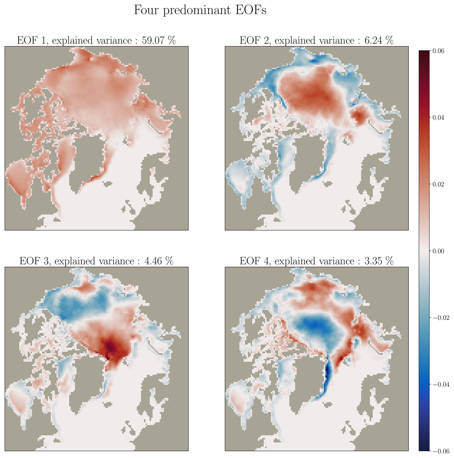
Figure B1 Four predominant EOFs of SIT, at the top left of each EOF is indicated the associated explained variance.

The four predominant EOFs are displayed in Fig. B1, as well as their associated variance.

B2 Choice of the truncation index m

In order to validate the best truncation index, we run an experiment with 4D–Var-EOF, in the twin experiment setup, with a value of m ranging from 10 to 8871. We then compute the total RMSE over all cycles. Results are presented in Fig. B2. We observe that for m>5000, the RMSE has reached a minimum. Let us note that using a smaller value of m reduces the minimization time, as it is reducing the dimension of the minimization space.

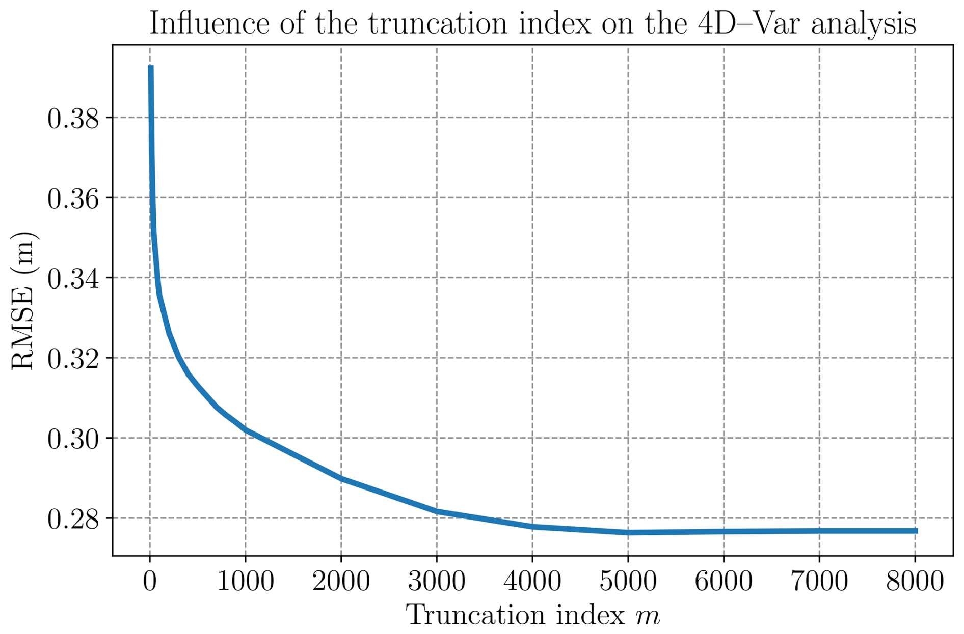
Figure B2 Average of the RMSE between x_a and x_t across all cycles and all timesteps for different values of k with Gaussian noise for the observations, in twin experiments and in the 4D–Var-EOF case.

Based on these results, and while we wanted to maintain a good reconstruction capacity, we chose to maintain m=7000 for all experiments.

Appendix C: 4D–Var optimization

C1 4D–Var algorithms

We present here the algorithms for the computation of the 4D–Var optimization, in the 4D–Var-EOF case. The computation of the cost function, for a given cycle, is shown in Algorithm C1. The state w₀ (projected onto the EOFs) is mapped back to the physical space, forecasted throughout the DAW using the emulator, where the observation term of the cost function is computed and then transformed back into the affine space of the EOFs. The total computation across all cycles is presented in Algorithm C2.

The L-BFGS-B (Broyden, 1967; Liu and Nocedal, 1989) algorithm is used to minimize the cost function 𝒥, defined in Algorithm C1. The optimization is constrained by bounds defined over all the variables of $\stackrel{\mathrm{̃}}{\mathit{x}}$ with a minimal value set to SIT_min as defined previously, in the case of the 4D–Var-diag. Two criteria are used to stop the minimization: f_tol, which corresponds to a threshold below which the cost function improvement is considered sufficient, and a gradient norm threshold g_tol, below which the norm of the gradient must fall. Note that we did not define a maximal number of iterations of the L-BFGS-B and the criteria f_tol was systematically reached.

In practice, in our case the only stopping criterion used is f_tol, as the gradient is significantly decreasing, yet, some instabilities at each iteration, especially on the MIZ are still observed, see Fig. C2.

C2 Cost function diagnostics

The value of the cost function 𝒥 as defined in Eq. (6b) or (9) and minimized with a L-BFGS-B can be followed across all cycles, as shown in Fig. C1. The RMSE increase observed in Fig. 4 can also be observed in the cost function. The increase in May comes after 9–10 cycles, which corresponds to 2 cycles before the time where the observation cost function decreases and the background cost function increases and becomes predominant. Based on this observed seasonality, we introduce an adaptive background-error strategy to offer an estimation of the order of magnitude of the background cost function. This implementation is further described in Appendix E.

Algorithm C1 Cost function (𝒥) computation for the 4D–Var-EOF.

Require:

g_θ, w₀, ${\stackrel{\mathrm{̃}}{\mathbf{y}}}_{k:\mathrm{1},\mathrm{\dots },K}$, the number of application of the emulator between two observations N_f, K, σ_obs, λ_inf, H, φ_m, F

${\mathcal{J}}_{\mathrm{b}}=\frac{\mathrm{1}}{\mathrm{2}{\mathit{\lambda }}_{\inf }^{\mathrm{2}}}({\mathbf{w}}_{\mathrm{0}}-{\mathbf{w}}_{\mathrm{0}}^{\mathrm{b}}{)}^{\top }({\mathbf{w}}_{\mathrm{0}}-{\mathbf{w}}_{\mathrm{0}}^{\mathrm{b}})$

𝒥_o=0

${\stackrel{\mathrm{̃}}{\mathbf{x}}}_{\mathrm{0}}=\overline{\mathbf{x}}+{\mathit{\phi }}_m{\mathbf{w}}_{\mathrm{0}}$

for i in range $(\mathrm{1},\mathrm{\dots },K)$ do

${\stackrel{\mathrm{̃}}{\mathit{x}}}_i=g_{\mathit{\theta }}^{{\mathrm{N}}_{\mathrm{f}}}({\stackrel{\mathrm{̃}}{\mathit{x}}}_{i-\mathrm{1}},{\mathbf{F}}_{i-\mathrm{1}\to i})$

${\mathcal{J}}_{\mathrm{o}}={\mathcal{J}}_{\mathrm{o}}+\frac{\mathrm{1}}{\mathrm{2}{\mathit{\sigma }}_{\mathrm{obs}}^{\mathrm{2}}}\Vert {\stackrel{\mathrm{̃}}{\mathbf{y}}}_i-\mathbf{H}{\stackrel{\mathrm{̃}}{\mathit{x}}}_i{\Vert }^{\mathrm{2}}$

end for

$\mathcal{J}={\mathcal{J}}_{\mathrm{o}}+{\mathcal{J}}_{\mathrm{b}}$

Algorithm C2 Wrapper for cycling the 4D–Var-EOF, using the loss (𝒥) defined in Algorithm C1.

Require:

$g_{\mathit{\theta }}({\stackrel{\mathrm{̃}}{\mathbf{x}}}_{\mathbf{t}},\mathbf{F})$, ${\stackrel{\mathrm{̃}}{\mathbf{y}}}_{k:\mathrm{1},\mathrm{\dots },K}$, N_f, N_cycle, K, w₀, DOF, λ_inf, φ_m

for n in range $(\mathrm{1},\mathrm{\dots },{\mathrm{N}}_{\mathrm{cycle}})$ do

${\mathbf{w}}_{\mathrm{0},n}^{\mathrm{a}}=\mathrm{L}-\mathrm{BFGS}({\mathbf{w}}_{\mathrm{0},n},\mathrm{loss}({\mathbf{w}}_{\mathrm{0},n},{\stackrel{\mathrm{̃}}{\mathbf{y}}}_{k:\mathrm{1},\mathrm{\dots },K}\left)\right)$

${\stackrel{\mathrm{̃}}{\mathbf{x}}}_{\mathrm{0},n}^a=\overline{\mathbf{x}}+{\mathit{\phi }}_m{\mathbf{w}}_{\mathrm{0},n}^{\mathrm{a}}$

${\stackrel{\mathrm{̃}}{\mathit{x}}}_{{\mathrm{N}}_{\mathrm{f}}(n\to n+\mathrm{1})}^{\mathrm{a}}=g_{\mathit{\theta }}({\stackrel{\mathrm{̃}}{\mathit{x}}}_{\mathrm{0},n}^{\mathrm{a}},{\mathbf{F}}_{n\to n+\mathrm{1}})$

${\stackrel{\mathrm{̃}}{\mathit{x}}}_n^{\mathrm{b}},{\stackrel{\mathrm{̃}}{\mathit{x}}}_n^{\mathrm{0}}={\stackrel{\mathrm{̃}}{\mathit{x}}}_{{\mathrm{N}}_{\mathrm{f}}(n+\mathrm{1})}^{\mathrm{a}}$

${\mathbf{w}}_{\mathrm{0},n+\mathrm{1}}={\mathit{\phi }}_m^{\top }({\stackrel{\mathrm{̃}}{\mathit{x}}}_n^{\mathrm{0}}-\overline{\mathbf{x}})$

$n\leftarrow n+\mathrm{1}$

end for

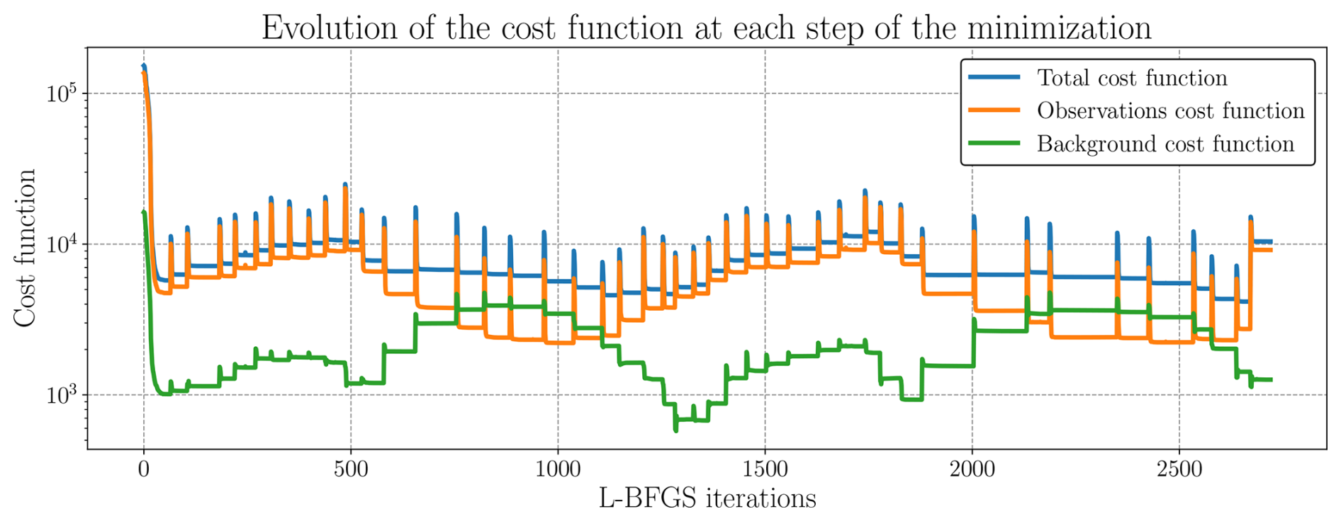
Figure C1 Cost function minimization with L-BFGS optimizer across all cycles for 4D–Var-EOF with log-normal noise, the total cost function is shown in blue, this term can be decomposed with the background loss term (green term) and the observation loss term (orange curve). Note that the y axis is in log scale.

C3 Gradient analysis

We can also investigate the gradient of the cost function, and its evolution between the beginning and the end of the cycle, as shown in Fig. C2. We can observe a global decrease of the gradient across the full Arctic. Yet, some grid-cells keep a strong gradient, especially on the MIZ.

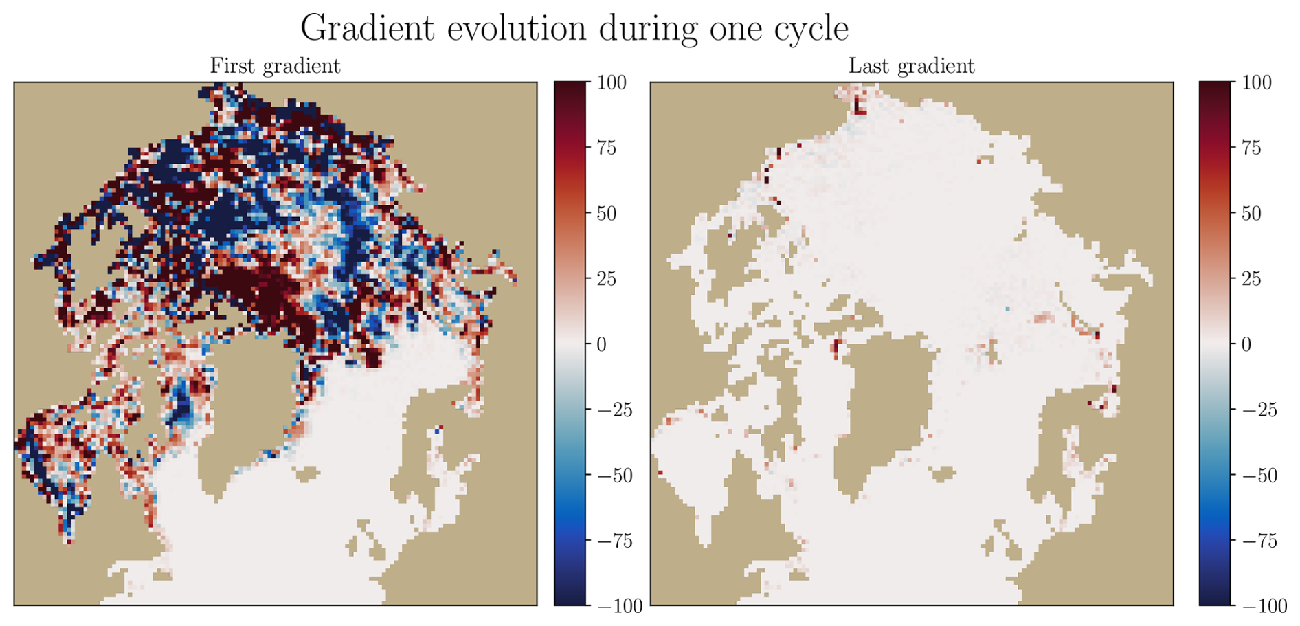
Figure C2 Evolution of the gradient during the 4D–Var-diag minimization. The left panel shows the gradient at the end of the first minimization of one cycle (cycle 31), while the right panel displays the gradient at the end of the last minimization of the same cycle, when the minimization criterion is reached. In this case, the synthetic observations are perfect observations (no noise addition).

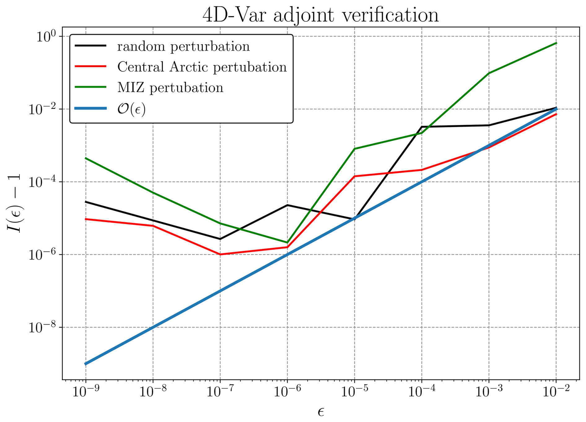
Figure C3 Logarithm of the absolute value of ℐ(ϵ) for several values of ϵ. Black line corresponds to the choice of a random perturbation of the cost function, with 10 experiments performed. Red line corresponds to a perturbation inside the Central Arctic region, with 5 experiments performed. Green line corresponds to a perturbation in the MIZ, with 5 experiments performed. Blue line corresponds to the identity $\mathcal{O}(\Vert \mathit{ϵ}\Vert )$.

C4 Tests of the emulator and the cost function gradients

First of all, we test the gradient of the cost function. With Taylor's expansion

$$\begin{array}{}\text{(C1)}& \mathcal{J}(x+\mathit{ϵ}h)=\mathcal{J}\left(x\right)+\mathit{ϵ}{\mathcal{J}}^{\prime }\left(x\right)\cdot h+\mathcal{O}(\Vert \mathit{ϵ}{\Vert }^{\mathrm{2}}),\end{array}$$

we look at the ratio

$$\begin{array}{}\text{(C2)}& \mathcal{I}\left(\mathit{ϵ}\right)=\langle \left|{\displaystyle \frac{\mathcal{J}(x+\mathit{ϵ}h)-\mathcal{J}(x-\mathit{ϵ}h)}{\mathrm{2}\mathit{ϵ}{\mathcal{J}}^{\prime }\left(x\right)\cdot h}}\right|{\rangle }_{\Vert h\Vert =\mathrm{1}},\end{array}$$

with x a state on the trajectory of the emulator. Note that we have

$$\begin{array}{}\text{(C3a)}& {\displaystyle }\mathcal{J}(x+\mathit{ϵ}h)& {\displaystyle }=\mathcal{J}\left(x\right)+\mathit{ϵ}{\mathcal{J}}^{\prime }\left(x\right)\cdot h+\mathcal{O}(\Vert \mathit{ϵ}{\Vert }^{\mathrm{2}})\text{(C3b)}& {\displaystyle }\mathcal{J}(x-\mathit{ϵ}h)& {\displaystyle }=\mathcal{J}\left(x\right)-\mathit{ϵ}{\mathcal{J}}^{\prime }\left(x\right)\cdot h+\mathcal{O}(\Vert \mathit{ϵ}{\Vert }^{\mathrm{2}}).\end{array}$$

By making the difference of those two equations we obtain

$$\begin{array}{}\text{(C4)}& \mathcal{J}(x+\mathit{ϵ}h)-\mathcal{J}(x-\mathit{ϵ}h)=\mathrm{2}\mathit{ϵ}{\mathcal{J}}^{\prime }\left(x\right)\cdot h+\mathcal{O}(\Vert \mathit{ϵ}{\Vert }^{\mathrm{2}}).\end{array}$$

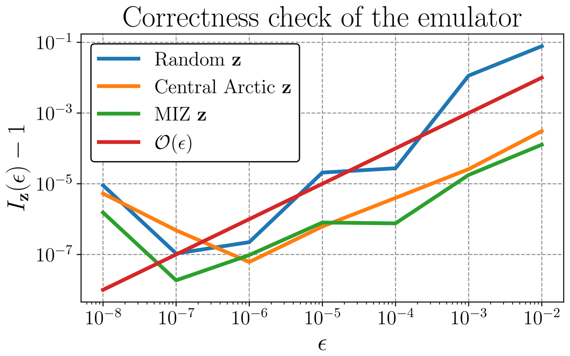
Figure C4 Logarithm of the absolute value of ℐ(ϵ) for several values of ϵ. Blue line corresponds to the choice of a random perturbation of the cost function, with 10 experiments performed. Orange line corresponds to a perturbation inside the Central Arctic region, with 5 experiments performed. Green line corresponds to a perturbation in the MIZ, with 5 experiments performed. Red line corresponds to the identity $\mathcal{O}(\Vert \mathit{ϵ}\Vert )$.

By averaging, we expect

$$\begin{array}{}\text{(C5)}& \mathcal{I}\left(\mathit{ϵ}\right)\simeq \mathrm{1}+\mathcal{O}(\Vert \mathit{ϵ}\Vert ).\end{array}$$

In practice, we take for the trajectory the full 2 years free run without assimilation, with the same parameters as defined in Sect. 5, with observations perturbed with cond-clipped noise. We evaluate several values h, including canonic vectors to focus only on single pixel, especially in the MIZ, and in Central Arctic. We define the canonic vectors h_zone∈ℝ⁸⁸⁷¹ as

$$\begin{array}{}\text{(C6)}& {\mathbf{h}}_{\mathrm{zone}}=(\mathrm{0},\mathrm{\cdots },\mathrm{0},\mathrm{1},\mathrm{0},\mathrm{\cdots },\mathrm{0}),\end{array}$$

with the 1 at the position corresponding to the chosen area. We select 5 pixels for the MIZ and 5 pixels for Central Arctic. The results are shown in Fig. C3. While the residual errors remain small, they increase for $\mathit{ϵ}<{\mathrm{10}}^{-\mathrm{7}}$. Above the ϵ value, we observe the expected behavior, but the residual errors are slightly noisy. Interestingly, we obtain similar behavior for the different values of h.

To test the gradient of the emulator, we evaluate the test function

$$\begin{array}{}\text{(C7)}& \mathcal{L}(\mathit{z},\mathbf{x})={\mathit{z}}^{\top }{g}_{\mathit{\theta }}(\mathbf{x},\mathbf{F}),\end{array}$$

whose Taylor's expansion in x is

$$\begin{array}{}\text{(C8a)}& {\displaystyle }\mathcal{L}(\mathit{z},\mathbf{x}+\mathit{ϵ}\mathbf{h})& {\displaystyle }={\mathit{z}}^{\top }{g}_{\mathit{\theta }}(\mathbf{x}+\mathit{ϵ}\mathbf{h},\mathbf{F})\text{(C8b)}& {\displaystyle }& {\displaystyle }=\mathcal{L}(\mathit{z},\mathbf{x})+\mathit{ϵ}{\mathit{z}}^{\top }{g}_{\mathit{\theta }}^{\prime }(\mathbf{x},\mathbf{F})\cdot \mathbf{h}+\mathcal{O}(\Vert \mathit{ϵ}{\Vert }^{\mathrm{2}})\end{array}$$

We study the ratio

$$\begin{array}{}\text{(C9)}& {\mathcal{I}}_{\mathit{z}}\left(\mathit{ϵ}\right)=\langle \left|{\displaystyle \frac{\mathcal{L}(\mathit{z},\mathbf{x}+\mathit{ϵ}\mathbf{h})-\mathcal{L}(\mathit{z},\mathbf{x}-\mathit{ϵ}\mathbf{h})}{\mathrm{2}\mathit{ϵ}{\mathit{z}}^{\top }{g}_{\mathit{\theta }}^{\prime }\left(\mathbf{x}\right)\cdot \mathbf{h}}}\right|{\rangle }_{\Vert h\Vert =\mathrm{1}},\end{array}$$

with x in the trajectory of the emulator. We expect the same behavior as for ℐ(ϵ). In this case, we look at several values for z, defined exactly as the previous h. The emulator is evaluated onto the full 2017–2018 dataset. Results are presented in Fig. C4. We obtain satisfying results, with a divergence of the residual for $\mathit{ϵ}<{\mathrm{10}}^{-\mathrm{8}}$. The curves for all different z vectors depict similar behavior, following the expected evolution in $\mathcal{O}(\Vert \mathit{ϵ}\Vert )$. The displacement in the MIZ and in Central Arctic yields lower residual results than with a random z vector.

Appendix D: Multi-year experiment

In this section, we present additional results showing the full two-year assimilation, including the one year spin-up cycles which are not included in the metrics computation. This shows the seasonality of the analysis RMSE, with increase during highly thermodynamics-driven period (spring melting and winter refreezing). The second part of the curve corresponds exactly to the RMSE shown in Fig. 4a), where the spring RMSE increase is also evident in 2017, confirming this recurrent behavior during periods of intense thermodynamic change. In addition, we note a pronounced peak in November 2017, coinciding with the refreezing period.

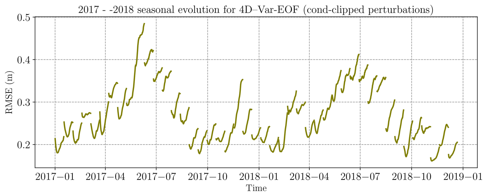
Figure D1 2017 and 2018 RMSE of 4D–Var-EOF in the twin experiment case, with cond-clipped perturbations. The curve represents the RMSE of the 4D–Var analysis with regard to neXtSIM SIT.

Appendix E: Background inflation

We adopt an adaptive multiplicative inflation scheme on the background error term, materialized by λ_inf,n and which is evaluated on each cycle n. It can be decomposed in two terms:

$$\begin{array}{}\text{(E1)}& {\mathit{\lambda }}_{\inf ,n}={\mathit{\lambda }}_{\mathrm{m}}\times {\mathit{\lambda }}_{\mathrm{a},n}.\end{array}$$

λ_m corresponds to the inflation term associated with the model error. It is constant throughout the experiments. In order to test the consistency of the solution of the innovation vector, we perform the ${\mathit{\chi }}_p^{\mathrm{2}}$ test. Under Gaussian assumption, the minimum value of the cost function has a ${\mathit{\chi }}_p^{\mathrm{2}}$ distribution with p the number of observations assimilated (Michel, 2014). It means that the average of the cost function minimum should stay around p, in our case $\mathrm{8871}\times {\mathrm{N}}_{\mathrm{obs}}/\mathrm{2}$, with N_obs the number of observations per window. Yet, with the different noise investigated in our study, this test does not work under other assumptions.

Following the χ² assumption, for each cycle, the minimal value of the cost function 𝒥 should in average be equal to the number of degree of freedom (DOF), which is equal to p. In practice, we define for each cycle n,

$$\begin{array}{}\text{(E2)}& {\mathit{\lambda }}_{\mathrm{a},n+\mathrm{1}}=\sqrt{{\displaystyle \frac{{\mathcal{J}}_{\mathrm{b}}^n}{|\mathrm{DOF}-{\mathcal{J}}_{\mathrm{o}}^n|}}},\end{array}$$

where ${\mathcal{J}}_{\mathrm{b}}^n$ corresponds to the background term of the cost function at cycle n and ${\mathcal{J}}_{\mathrm{o}}^n$ corresponds to the observation term of the cost function at cycle n; with, for the initial cycle, a value of 1 for λ_a,0.The multiplication of the two terms λ_m and λ_a,n gives us the total inflation λ_inf,n in the adaptive case.

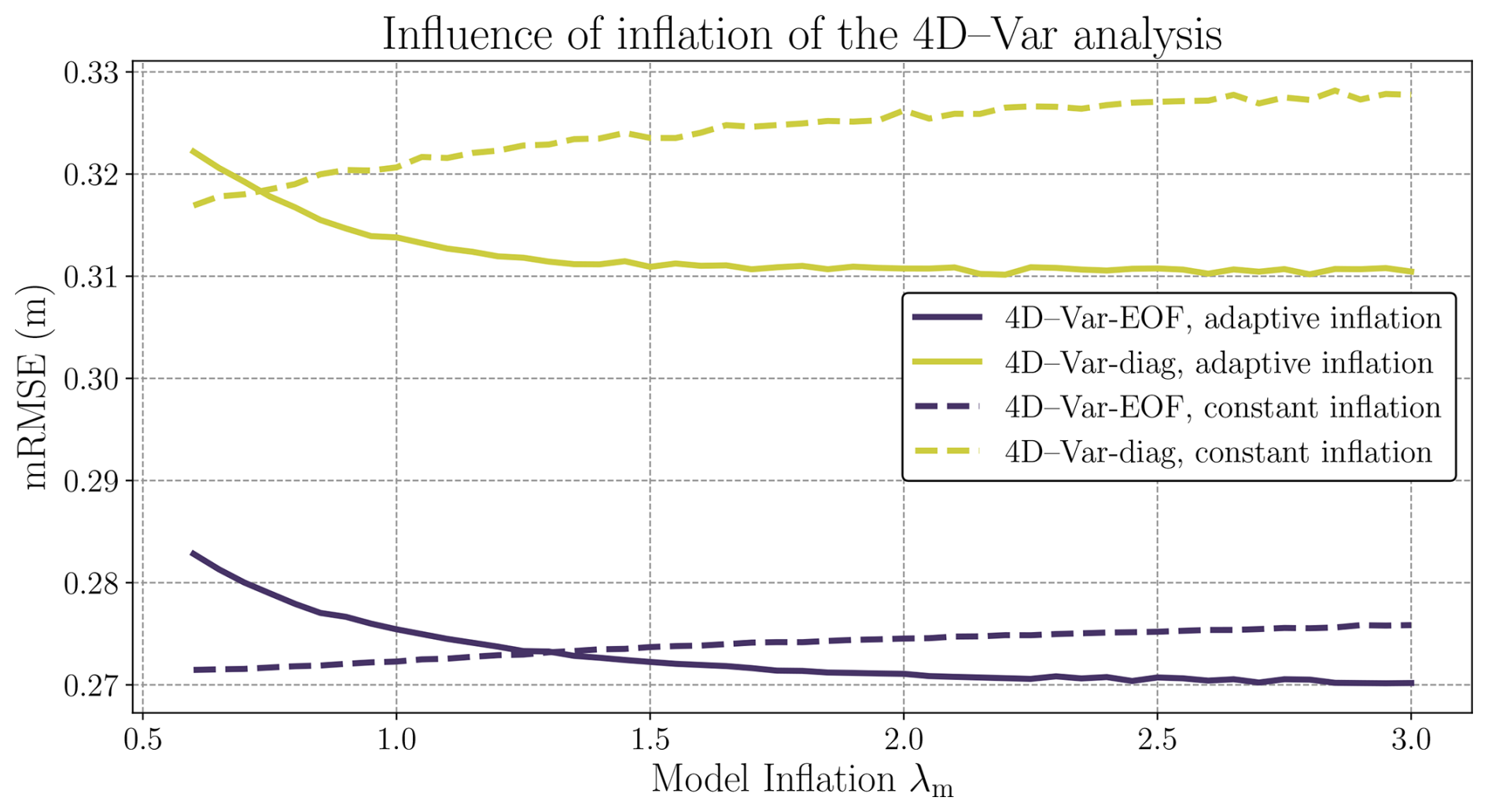
Figure E1 mRMSE of x_a for both 4D–Var-EOF (dark blue lines) and 4D–Var-diag (green lines), for the two types on background inflation proposed, the constant inflation (dashed lines) and the adaptive inflation (solid lines). The results are plotted as a function of the model inflation λ_m. In the case of the constant inflation, λ_a is automatically set to 1 whereas in the adaptive case, it is defined as per Eq. (E2).

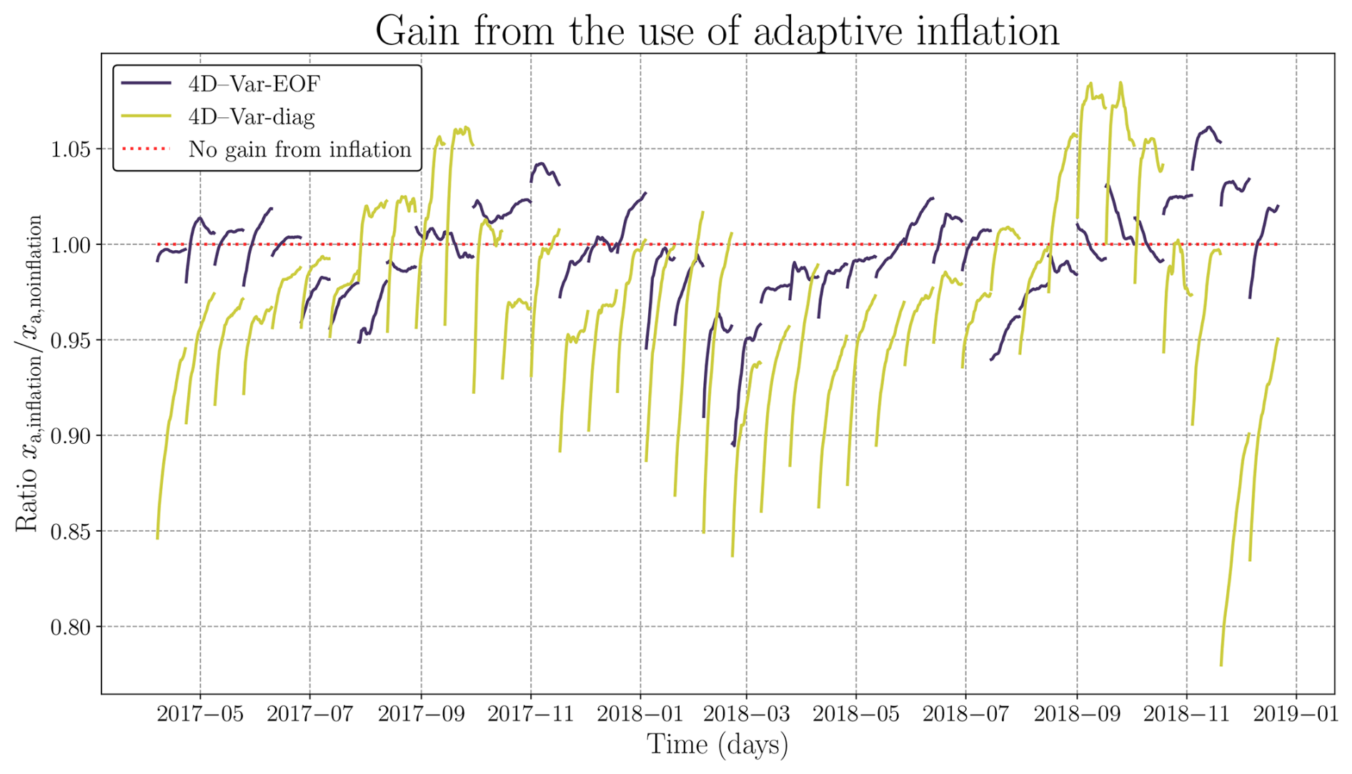
Figure E2 Evaluation of the gain from the adaptive inflation, compared to no inflation, for both 4D–Var-EOF (dark blue lines) and 4D–Var-diag (green lines). The ratio between the RMSE of x_a,inflation and x_{a,no inflation} is plotted with respect to time. The dotted red line indicates the position where there is no gain from the inflation. A value of this ratio below 1 means a gain from the adaptive scheme whereas a value above 1 corresponds to a loss in RMSEs.

In order to help the optimization of the 4D–Var, we investigate the use of inflation scheme as defined in Eq. (E2). Two schemes are evaluated, a constant inflation, only modeled by λ_m and an adaptive inflation scheme with the multiplication of λ_a based on the χ² estimation of 𝒥 and λ_m. Only Gaussian noise for the observations are considered and the value of λ_m ranges between 0.6 and 3. Results with the mRMSE are outlined in Fig. E1. As observed before we can see that 4D–Var-EOF is clearly better than 4D–Var-diag, but both inflation schemes have similar behavior in both cases. Using an inflation scheme (λ_inf≠1) yields better results in terms of mRMSE in both cases if we correctly tune λ_m. Interestingly, in the case of constant inflation, the mRMSE increases almost linearly with λ_m. This indicates that, when using constant inflation, emphasizing the 𝒥_o term tends to undermine the performance of the 4D–Var. Conversely, in the adaptive case, assigning a significant value to λ_m while still optimizing the ratio between 𝒥_b and 𝒥_o results in improved mRMSE.

As shown in Fig. E2, in which is plotted the ratio between the two analysis x_a,inflation and x_{a,no inflation}, with x_a,inflation the analysis with the adaptive inflation scheme with λ_m set to 3 and x_{a,no inflation} the analysis of the run with Gaussian noise without any inflation scheme, in 2018, we can see that the benefit from inflation is primarily observed at the start of the DAW and more prominently at the beginning of the year. On average, the gain from the adaptive inflation is mitigated, as some end of cycle ratio are above 1. By using the inflation, we favor the improvement at the beginning of the DAW to the detriment of the end of the DAW. Let us also note that the major gain from the inflation come from March to July, which corresponds to the period where the RMSE of the analysis x_a is higher.

To conclude, adaptive background inflation can be easily implemented in twin experiment scenarios. We observe a modest improvement in the total average RMSE, with most of the gains occurring at the beginning of the assimilation windows. In the case of adaptive inflation, the inflation values fluctuate around 0.5, exhibiting a seasonal pattern.