Using observations of surface fracture to address ill-posed ice softness estimation over Pine Island Glacier

Numerical models used to simulate the evolution of the Antarctic Ice Sheet require the specification of basal boundary conditions on stress and local deviations in the assumed material properties of the ice. In general, scalar fields relevant to these unknown components of the system are found by solving an inverse problem given observations of model state variables – typically ice flow speed. However, these optimisation problems are ill posed, resulting in degenerate solutions and poor conditioning. In this study, we propose the use of fracture and strain rate data to provide prior information to the inverse problem, in an effort to better constrain the inferred ice softness compared to more heuristic regularisation techniques. We use Pine Island Glacier as a case study and consider both a snapshot inverse problem in which ice softness and basal slip parameters are sought simultaneously over the glacier as a whole, and a time-dependent problem in which ice softness alone is sought over the floating ice shelf at regular intervals. In the first case, we construct a prior encoding the assumption that the ice softness will be close to our initial guess except from where we see fractures or high shear strain rates in satellite data. We investigate the solutions and conditioning of this data-informed inverse problem versus alternatives. The second proposed method makes the assumption that changes to ice softness occurring on monthly-to-annual timescales will be dominated by the fracturing of ice. We show that these methods can result in softness fields on floating ice that visually mimic fracture patterns without significantly affecting the solution misfit, perhaps leading to greater confidence in the softness fields as a representation of the true material properties of the ice shelf.

1 Introduction

Large-scale ice sheet models commonly treat ice within the paradigm of continuum mechanics – as a shear thinning viscous fluid; an approach that has been successful in modelling the behaviour of large ice masses relatively cheaply (e.g. Seroussi et al., 2020). Within this framework, the flow of the ice can be accounted for in large part by a balance between gravity, viscous stress due to internal deformation and frictional stress at ice/bedrock interfaces. To close the system and allow the model to solve for ice speed, equations relating viscous and frictional stresses to ice speed are specified, informed by laboratory data and physical arguments.

The former “constitutive relation” very often takes the form of Glen's flow law:

$$\begin{array}{}\text{(1)}& {\mathit{\tau }}_{ij}=\mathrm{2}\mathit{\eta }{\dot{\mathit{\epsilon }}}_{ij}\text{ where }\mathit{\eta }={\displaystyle \frac{\mathrm{1}}{\mathrm{2}}}A(T{)}^{-\frac{\mathrm{1}}{n}}{\mathit{ϵ}}^{\frac{\mathrm{1}}{n}-\mathrm{1}}\end{array}$$

where τ_ij is the deviatoric stress tensor, ${\dot{\mathit{\epsilon }}}_{ij}$ is the strain rate tensor, ϵ is its second invariant, η is the strain-rate-dependent effective ice viscosity and A(T) is a temperature-dependent rate factor. The value of the exponent n is dependent on the particular mechanisms by which creep occurs within the ice and various properties of the crystal grains (e.g. Haefeli, 1961), and takes a value between 1 and 4 in most cases. (Here, we take the common reference value of n=3.) It is possible to treat A(T) and/or n as free parameters that can be fitted to observations, given the uncertainties involved in both and the different physical mechanisms that distinguish them. Frequently, however, these are prescribed a priori and a stiffness field ϕ(x) is defined over the domain to account for unknown deviations in the expected ice rheology. As such, Eq. (1) becomes ${\mathit{\tau }}_{ij}=\mathrm{2}\mathit{\varphi }\mathit{\eta }{\dot{\mathit{\epsilon }}}_{ij}$. Used in this way, ϕ approximates the effect of uncertainties in the temperature and thickness fields, regional changes in the temperature dependence of Glen's flow law, deviations from the assumed isotropy of creep deformation and, of particular interest to this study, fractures in the ice at different lengthscales. Often, a softness field φ is defined in relation to the stiffness field by $\mathit{\phi }=(\mathrm{1}-\mathit{\varphi })$.

The relation between frictional stress and basal sliding speed is known as a sliding law, and has a functional form that depends on a number of often poorly constrained factors such as the expected amount of deformation of ice around topographic features in the bed, sliding over smooth bedrock, and shearing of the sub-glacial till. A single sliding law is often combined with a spatially varying basal slip parameter C(x) to approximate this stress:

$$\begin{array}{}\text{(2)}& {\mathit{\tau }}_{\mathrm{b}}=Cf\left(\mathit{u}\right).\end{array}$$

Given a constitutive relation and sliding law defined as above, the equations solved by most large-scale ice sheet models contain a component dependent on ϕ (or a related scalar field performing an equivalent role) that represents viscous stress, a component dependent on C that represents frictional stress, and a component representing gravitational driving. Therefore, for an ice sheet model to simulate real ice masses accurately, these scalar fields must be well-constrained. In practice, they are typically inferred simultaneously from observations of ice speed using inverse methods – a suite of techniques for inferring model control parameters from observed state variables (MacAyeal, 1992) – (e.g. Petra et al., 2012; Arthern et al., 2015; Cornford et al., 2015; Gudmundsson et al., 2019). Ice velocity data, rather than ice speed data, is also widely used in the community, and some methods of establishing current values for C and ϕ also incorporate rates of thickness change into the inverse problem (e.g. Larour et al., 2014; Goldberg et al., 2015) (though this relies on the model having an automatically differentiable forward solver). We don't explicitly consider these latter kinds of “transient” inverse problem here, though the arguments we present still apply.

Regardless of its precise implementation, this inverse problem is ill-posed, resulting in solutions that are degenerate and highly dependent on noise in the input data (the problem, at least in its discrete form, is ill-conditioned). To obtain reliable control fields, it is beneficial to replace this ill-posed problem with a nearby well-posed one before solving it. The problem is sometimes simplified by solving for C only on grounded ice, and ϕ on floating ice, thereby separating the two fields spatially and removing a portion of the degeneracy that arises from the mixing of these fields (e.g. Goldberg et al., 2019). However, though you would often expect C to be the dominant control on grounded ice speed, this may well not be true everywhere and an incorrect guess for ϕ could have consequences for transient simulations. Another approach is to regularise the solution by providing additional constraints on the control fields. Such a regularised inverse problem takes the general form of the following optimisation:

$$\begin{array}{}\text{(3)}& \begin{array}{rl}(C,\mathit{\varphi })& =\underset{C,\mathit{\varphi }}{argmin}\left\{{\mathcal{J}}_{\mathrm{m}}(u,u_o)+{\mathit{\alpha }}_C{\mathcal{J}}_C\left(C\right)+{\mathit{\alpha }}_{\mathit{\varphi }}{\mathcal{J}}_{\mathit{\varphi }}\left(\mathit{\varphi }\right)\right\},\\ & \text{s.t.}G(u,C,\mathit{\varphi })=\mathrm{0}\end{array}\end{array}$$

where 𝒥_m(u,u_o) is a misfit functional calculating the distance of the model output u from the observed data u_o (often ice speed), 𝒥_C and 𝒥_ϕ are regularisation terms for the C and ϕ fields, with strengths controlled by the parameters α_C and α_ϕ respectively, and $G(u,C,\mathit{\varphi })=\mathrm{0}$ are the momentum balance equations solved in the model's forward problem.

A popular approach, aimed at improving the conditioning of the problem by suppressing the amplification of high-frequency components of the input data, is to use Tikhonov regularisation in a form that favours either low spatial frequency or low amplitude components of the solution (e.g. Morlighem et al., 2013; Habermann et al., 2013; Brinkerhoff and Johnson, 2013; Cornford et al., 2015), e.g.:

$$\begin{array}{}\text{(4)}& {\mathit{\alpha }}_{\mathit{\varphi }}{\mathcal{J}}_{\mathit{\varphi }}\left(\mathit{\varphi }\right)={\mathit{\alpha }}_{\mathit{\varphi }}\underset{\mathrm{\Omega }}{\int }|\mathrm{\nabla }\mathit{\varphi }{|}^{\mathrm{2}}\mathrm{d}\mathrm{\Omega }.\end{array}$$

However, this kind of regularisation is entirely heuristic and, when it comes to distinguishing C and ϕ, relies on assumed differences in the lengthscales over which changes in the control fields can influence strain rates. Generally, in regions without significant shear, these lengthscales are not easily distinguished, and degeneracies between solutions for C and ϕ proliferate. Additional difficulties arise when a control field contains distinct contributions with different spatial frequencies. For example, uncertainty in englacial temperature can vary on the scales of long-term atmospheric or geothermal heat sources, or over the width of a shear margin. Often, an imperfect but acceptable lengthscale is found by searching parameter space informed by heuristics such as L-curve analysis (Hansen and O'Leary, 1993; Hansen, 1994).

The aim of this study is to investigate whether the introduction of genuine prior information into the inverse problem results in solutions that are more qualitatively appealing than those found using other, heuristic regularisation methods.

Previous studies have investigated instances in which softness fields found through solving inverse problems have mirrored observed fracture features (Borstad et al., 2013; Surawy-Stepney et al., 2023a) – suggesting that the presence of fractures has the potential to dominate ϕ. With recent advancements in observational methods for locating fractures in remote sensing data (Lai et al., 2020; Izeboud and Lhermitte, 2023; Zhao et al., 2022; Surawy-Stepney et al., 2023b), we are moving towards reliable data that can be used to inform us at least about this specific component of the softness field. Ranganathan et al. (2021) showed previously that the use of strain rate data to weight the regularisation of C and ϕ has the potential to reduce mixing between these control fields. The work presented here follows quite naturally from these results.

Here, we investigate two ways in which fracture and strain-rate observations can be used to inform the inverse problem to replace or complement existing heuristic methods. The first is to use maps of surface fracture along with estimates of surface strain-rates to construct a prior distribution for ϕ for use in snapshot inverse problems (single optimisations carried out for a set of geometry and speed data collected at a specific instant in time). Next, we investigate the use of timeseries of fracture maps in constraining the solutions to inverse problems carried out over multiple timesteps on floating ice. We make the assumption that softness fields should vary on long timescales except from where we see changes to the pattern of fracture. We show, with these methods, that one can generate softness fields that mimic, in certain ways, the changing fracture patterns on the Pine Island Ice Shelf between 2016 and 2021, without substantially affecting the solution misfit. This may have potential uses in constraining models that aim to evolve softness fields in response to englacial stresses.

2 Methods

The simulations presented in this article were performed using the BISICLES ice sheet model (Cornford et al., 2013). This is an adaptive mesh, finite volume model which we choose here to solve discretized versions of the two-dimensional shallow-stream equations:

$$\begin{array}{}\text{(5)}& \begin{array}{rl}\mathrm{\nabla }& \cdot \left[\mathit{\varphi }h\overline{\mathit{\eta }}\right(\mathrm{\nabla }\mathit{u}+(\mathrm{\nabla }\mathit{u}{)}^{\top }+\mathrm{2}(\mathrm{\nabla }\cdot \mathit{u}\left)\mathcal{I}\right)]\\ & -Cf\left(\mathit{u}\right)-{\mathit{\rho }}_{i}gh\mathrm{\nabla }s=\mathrm{0},\end{array}\end{array}$$

where $\mathit{u}=(u_x,u_y{)}^{\top }$ is the horizontal velocity, $\overline{\mathit{\eta }}$ is the vertically-integrated effective ice viscosity, ρ_i is the density of ice, h is the ice thickness and s is the ice surface. In this study we use a linear sliding law f(u)=u for ease of computing adjoint sensitivities during the inverse problem.

Each inverse problem we consider in this article is of the form of Eq. (3), with a misfit functional of the form ${\mathcal{J}}_{\mathrm{m}}(u,u_o)=\Vert u-u_o{\Vert }_{\mathrm{2}}^{\mathrm{2}}$. The inverse problems differ solely in the form of the regularisation terms 𝒥_ϕ. We solve each in BISICLES using a non-linear conjugate gradient method (Cornford et al., 2015).

Each simulation is carried out over Pine Island Glacier (PIG) in the Amundsen Sea Sector of West Antarctica with a domain encompassing the whole present-day drainage basin (Zwally et al., 2012). This region was chosen as it represents a potentially strong correspondence between fracturing and ice softness, given the abundant crevasses in the shear margins, upstream of the grounding line and the regular formation of rifts near the terminus, as well as the established dynamic impact of some of this fracturing (Joughin et al., 2021; Sun and Gudmundsson, 2023). Across the rest of Antarctica, we expect the link between the dynamics of ice and the extent of fracturing to be weaker in general – due to the lack of obviously coincident changes in fracture and ice dynamics. We use a form of the rate factor A(T) described in Cuffey and Paterson (2010), with an internal energy field generated using a 100 000 year calculation in which surface temperature, thickness and velocity are held at present day values and the combined ice temperature and moisture fraction field $E=CT+Lw$ evolves toward equilibrium. We used a geometry defined by BedMachine-v3 (Morlighem, 2022), with time-evolving calving front positions extracted from Sentinel-1 backscatter images. Each simulation used velocity and fracture data from within a five-year period between November 2016 and November 2021. We used 200 m resolution, monthly-averaged ice velocity observations made using feature tracking applied to Sentinel-1 image pairs (Wuite et al., 2021) as the input data to the cost function and to estimate shear strain rates.

Crevasse data were generated according to the methods described in Surawy-Stepney et al. (2023b). This involves the application of deep-learning-based and other computer vision techniques to synthetic aperture radar (SAR) backscatter images from the Sentinel-1 satellite clusters, at 50 m spatial resolution. This produces maps showing the locations at which the surface expressions of crevasses and rifts are visible in the SAR data and include crevasses on floating and grounded ice. Of particular interest to this study are rifts on the Pine Island ice shelf, fractures in its shear margins, and the large field of grounded crevasses extending ∼100 km upstream of the grounding line (Fig. 1a). We use composite fracture maps that combine data from a month of SAR backscatter images, taking into account the differing visibility of crevasses imaged from different angles. The presence of obliquely overlapping Sentinel-1 frames is another reason for the choice of PIG as the location for this study.

2.1 Fracture data assimilation in snapshot inverse problems

The snapshot problem we consider is the joint estimation of C and ϕ over Pine Island Glacier in May 2019 from mean ice speeds over the month.

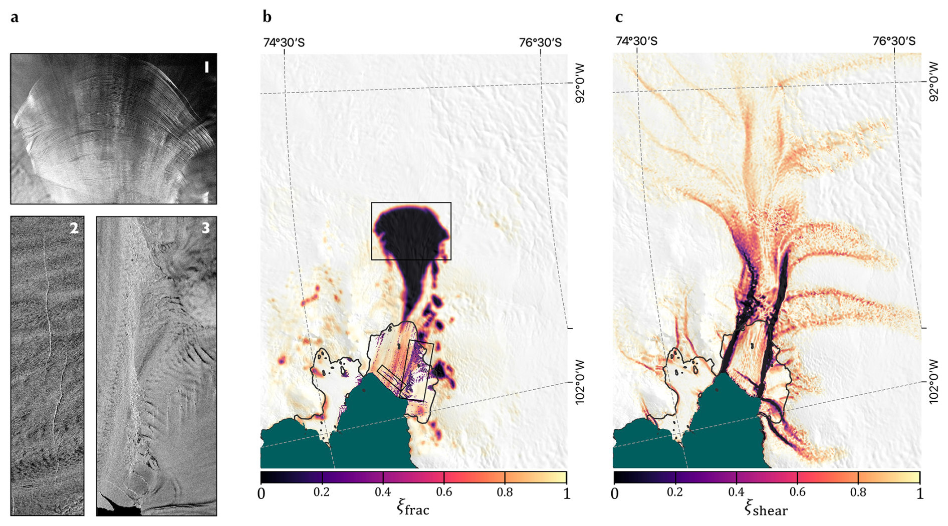
Figure 1 Contributions to the field ξ, representing, in our prior for the softness field, where we have observations of surface fracture or high shear strain rates. (a) SAR backscatter images over grounded and floating parts of Pine Island Glacier from May 2019 showing regions of visible crevassing: (1) surface crevasses on the grounded ice, (2) two almost-connected rifts near the Pine Island calving front, (3) the heavily “damaged” southern shear margin of Pine Island Ice Shelf. (b) The component of ξ due to the observation of crevasse features, made from fracture maps developed in Surawy-Stepney et al. (2023b). Black boxes anticlockwise from the top show the locations of the SAR images a1, a2 and a3 respectively. (c) The component of ξ due to the presence of high shear strain rates. Background images to b and c are the MODIS Mosaic of Antarctica (Haran et al., 2021), and grounding lines (shown in black) are according to Rignot et al. (2016).

The prior we construct for ϕ encodes the assumption that ϕ≈1 away from regions of observed fracture or where there are high shear strain rates (which can contribute the effects of enhanced anisotropy, shear heating and microfracturing to ϕ). In practise, this is equivalent to a form of Tikhonov regularisation using a diagonal Tikhonov matrix with entries weighted away from where we expect soft ice.

To construct this, we first form a field ξ which goes to 0 in regions which have high shear strain rates (defined below) or where fractures have been observed and to 1 elsewhere. In essence, this should reflect our confidence in our initial guess for the ice rheology. We construct it as:

$$\begin{array}{}\text{(6)}& \mathit{\xi }=\text{min}\mathit{\{}{\mathit{\xi }}_{\mathrm{frac}},{\mathit{\xi }}_{\mathrm{shear}}\mathit{\}}\end{array}$$

where ξ_frac is low where we see fractures in satellite imagery (Fig. 1b), and ξ_shear is low where we see high strain rates (Fig. 1c).

To construct ξ_frac, we first smooth the fracture map for May 2019, by convolving with a Gaussian kernel, to produce contiguous fracture fields on the grounded ice. We call this fracture map f. Then ${\mathit{\xi }}_{\mathrm{frac}}=\mathrm{1}-f$ (Fig. 1b). There are a few things to note in these fracture data of potential relevance to the stress-balance of the glacier. Firstly, we see a large contiguous area of surface fractures extending upstream from the grounding line and widening to cover a region in which previous studies have suggested membrane stresses are important in the stress-balance as basal stresses become small (Joughin et al., 2009) – something we see in our own solutions for basal stress. SAR images of this region show uniform coverage by closely-spaced surface fractures, almost identical in appearance (Fig. 1a1). If this is indeed an area in which membrane stresses form a significant component of the stress balance, the presence of crevasses deeper than the firn layer could have implications for the dynamics by changing the horizontal transmission of stress. Additionally, there is a rift (really, two rifts that are almost connected) near to the ice shelf terminus that led to the calving of a large tabular iceberg in February 2020 (Fig. 1a2) – part of a series of calving events regarded to have had significant consequences for the dynamics of Pine Island Glacier (Joughin et al., 2021). Finally, there are a large number of fractures on the southern shear margin of Pine Island Ice Shelf (Fig. 1a3). Viscous deformation in shear margins can account for a significant portion of the stress budget of an ice shelf, so changes to the large-scale rheology in such locations will influence the distribution of stress throughout the ice shelf.

We create ξ_shear, the strain-rate contribution to ξ, using the same velocity data that we use in our misfit functional. To estimate the derivatives ∂_iu_j, we differentiated the velocity components using a method described in Chartrand (2017), using Tikhonov regularisation to promote smoothness (regularisation parameters were chosen with some trial-and-error, where preference was given to solutions in which regions of high shear varied smoothly over lengthscales comparable to the widths of visible shear margins). Aligning the x-coordinate with local flow direction, we define regions of high shear to be those in which $\left|{\dot{\mathit{\epsilon }}}_{xy}\right|>\mathrm{0.1}$ a⁻¹. This threshold is a bit discretionary, though it corresponds to stresses within the range 90–320 kPa of tensile strength suggested in Vaughan (1993) for a wide range of englacial temperatures. Then ${\mathit{\xi }}_{\mathrm{shear}}=max\mathit{\{}\mathrm{0},\mathrm{1}$–$\mathrm{10}\left|{\dot{\mathit{\epsilon }}}_{xy}\right|\mathit{\}}$ (Fig. 1c) and $\mathit{\xi }=\text{min}\mathit{\{}{\mathit{\xi }}_{\mathrm{frac}},{\mathit{\xi }}_{\mathrm{shear}}\mathit{\}}$ (this looks like a combination of Fig. 1b and c).

In the case of the snapshot inverse problem, the assumption we wish to encode is that $\mathit{\varphi }\sim \mathcal{N}(\mathrm{1},{\mathit{\gamma }}^{\mathrm{2}})$ whenever ξ→1, where γ is a small number related to the strength of the prior. This can be written:

$$\begin{array}{}\text{(7)}& p_{\mathrm{\Phi }}\left(\mathit{\varphi }\right)\propto \text{exp}\left(-{\displaystyle \frac{\mathrm{1}}{\mathrm{2}{\mathit{\gamma }}^{\mathrm{2}}}}\underset{\mathrm{\Omega }}{\int }(\mathrm{1}-\mathit{\varphi }{)}^{\mathrm{2}}\mathit{\xi }\mathrm{d}\mathrm{\Omega }\right).\end{array}$$

Assuming the distribution of measurement errors is isotropic, with covariance σ²ℐ, this translates to a regularisation term:

$$\begin{array}{}\text{(8)}& {\mathit{\alpha }}_{\mathit{\varphi }}={\displaystyle \frac{{\mathit{\sigma }}^{\mathrm{2}}}{{\mathit{\gamma }}^{\mathrm{2}}}},{\mathcal{J}}_{\mathit{\varphi }}\left(\mathit{\varphi }\right)=\underset{\mathrm{\Omega }}{\int }(\mathrm{1}-\mathit{\varphi }{)}^{\mathrm{2}}\mathit{\xi }\mathrm{d}\mathrm{\Omega }.\end{array}$$

To understand how the introduction of prior information in the form of crevasse and strain-rate data changes the solutions to the inverse problem, we compare the solutions to those found using alternative regularisation methods. For the snapshot case, we perform three inverse problems over the full domain, starting with the same initial guesses for C and ϕ, with the same regularisation on C, with the following regularisation terms for ϕ, defined in reference to Eq. (3):

1. No regularisation: 𝒥_ϕ(ϕ)=0.

2. The widely-used heuristic regularisation: ${\mathcal{J}}_{\mathit{\varphi }}\left(\mathit{\varphi }\right)={\int }_{\mathrm{\Omega }}|\mathrm{\nabla }\mathit{\varphi }{|}^{\mathrm{2}}\mathrm{d}\mathrm{\Omega }$.

3. Our data-informed regularisation: ${\mathcal{J}}_{\mathit{\varphi }}\left(\mathit{\varphi }\right)={\int }_{\mathrm{\Omega }}(\mathrm{1}-\mathit{\varphi }{)}^{\mathrm{2}}\mathit{\xi }\mathrm{d}\mathrm{\Omega }$

The results are shown in Sect. 4.1.

We note that the initial guess for the control fields can have a large influence on the optimisation problem, as the closer it is to the desired solution, the more likely it is that the optimisation will converge close to that solution. For the ϕ field, we use an initial guess of 1 everywhere (this is likely to be within an order of magnitude of the solution). The C field can vary by orders of magnitude, so a uniform initial guess would be a poor choice. Instead, we take the view that the initial guess should be the field required to reproduce the observations on grounded ice as closely as possible with a uniform ϕ=1. This is reflective of an assumption that grounded ice speed is largely accounted for by balance between gravity and friction (though we know this to be untrue). Hence, before carrying out the full optimisation including both control fields, we solve an inverse problem for C with fixed ϕ=1, matching speeds only on grounded ice and use this as the initial guess for the joint inverse problem. This has the effect of reducing the deviation of ϕ from 1 in the solution and has the added bonus of allowing us to search independently for the regularisation parameters α_C and α_ϕ. In general, we carry out the search for regularisation parameters using L-curve analysis (Hansen and O'Leary, 1993), though we consider this a heuristic method that should be used alongside other methods where necessary (Sect. 5.3).

2.2 Fracture data assimilation through time

The use of fracture maps as a prior in the snapshot inverse problems makes an assumption about the relative contributions of different uncertainties to ϕ. For example, we have to have a certain amount of trust in the 3D temperature field we use. As previously noted, ϕ also contains contributions from sources that cannot easily be distinguished by the spatial scales on which they vary. However, it seems likely that the contribution of fracturing to ice softness varies on a shorter temporal scale than any other contribution. Hence, while attributing ice softness to the presence of fractures requires a large number of assumptions, we can reasonably attribute changes in ice softness over monthly-to-annual timescales to the fracturing or healing of ice, and the advection of fractures. With this in mind, we consider the case of imposing a regularisation that penalises changes to ϕ in successive timesteps, except where we have seen the evolution of fractures in the observational data. Concretely, given a series of timesteps with times $\mathit{\left\{}{t}_i\right|i=\mathrm{1},\mathrm{\dots },n\mathit{\}}$, separated by Δt (e.g. one month), we solve the following inverse problem for the control parameters (C_i,ϕ_i) at each timestep:

$$\begin{array}{}\text{(9)}& \begin{array}{rl}(C_i,{\mathit{\varphi }}_i)& =\underset{C_i,{\mathit{\varphi }}_i}{argmin}\mathit{\left\{}{\mathcal{J}}_{\mathrm{m}}\right(u_i,u_{o_i})+{\mathit{\alpha }}_C{\mathcal{J}}_C(C_i)\\ & +{\displaystyle \frac{{\mathit{\alpha }}_{\mathit{\varphi }}}{\mathrm{\Delta }t}}{\mathcal{J}}_{\mathit{\varphi }}({\mathit{\varphi }}_i,{\mathit{\varphi }}_{i-\mathrm{1}})\mathit{\}},\end{array}\end{array}$$

This is much the same as the snapshot inverse problem defined by Eq. (3), though our regularisation term ${\mathcal{J}}_{\mathit{\varphi }}({\mathit{\varphi }}_i,{\mathit{\varphi }}_{i-\mathrm{1}})$ now includes the softness fields in the current and previous timesteps. Though not particularly sophisticated, a method such as described by Eq. (9) is immediately amenable to the introduction of fracture data through its inclusion in the regularisation term 𝒥_ϕ. Previous studies (Hogg et al., 2017; Selley et al., 2021) have used such a method with ${\mathcal{J}}_{\mathit{\varphi }}={\int }_{\mathrm{\Omega }}|{\mathit{\varphi }}_i-{\mathit{\varphi }}_{i-\mathrm{1}}{|}^{\mathrm{2}}\mathrm{d}\mathrm{\Omega }$ and we modify this only slightly here. We propose the regularisation function:

$$\begin{array}{}\text{(10)}& {\mathcal{J}}_{\mathit{\varphi }}=\underset{\mathrm{\Omega }}{\int }(\mathrm{1}-|f_i-f_{i-\mathrm{1}}\left|\right)\times |{\mathit{\varphi }}_i-{\mathit{\varphi }}_{i-\mathrm{1}}{|}^{\mathrm{2}}\mathrm{d}\mathrm{\Omega }\end{array}$$

where f_i is the map showing the locations of fractures over the domain at time t_i. Hence, changes to the softness field are preferred in regions in which the fracture pattern has changed, with a strength that depends on the length of the timestep and the regularisation parameter α_t.

We carry out such a procedure on Pine Island Glacier with 5 years of speed and fracture observations from December 2016 to December 2021, and timesteps of one month. This captures three calving events and the major disintegration of the southern shear margin of the ice shelf, and that of the calving front of Piglet Glacier (Joughin et al., 2021; Surawy-Stepney et al., 2023b). For each month, we use the mean speeds measured over that month as our observed speeds, and median fracture map composites.

We carry out two series of inverse problems, both starting with the same initial guess (ϕ field found using heuristic regularisation). One to act as a baseline, and the other reflecting our new approach:

1. Heuristic regularisation: ${\mathcal{J}}_{\mathit{\varphi }}={\int }_{\mathrm{\Omega }}|{\mathit{\varphi }}_i-{\mathit{\varphi }}_{i-\mathrm{1}}{|}^{\mathrm{2}}\mathrm{d}\mathrm{\Omega }$.

2. Data-informed regularisation: ${\mathcal{J}}_{\mathit{\varphi }}={\int }_{\mathrm{\Omega }}(\mathrm{1}-|f_i-f_{i-\mathrm{1}}\left|\right)\times |{\mathit{\varphi }}_i-{\mathit{\varphi }}_{i-\mathrm{1}}{|}^{\mathrm{2}}\mathrm{d}\mathrm{\Omega }$

The results for these simulations are shown in Sect. 4.2.

3 A synthetic example

In order to validate the basic premise of the method and build some intuition as to where we could expect it to change the solution, we performed some preliminary synthetic experiments involving the heuristic and data-informed regularisations of the snapshot inverse problem.

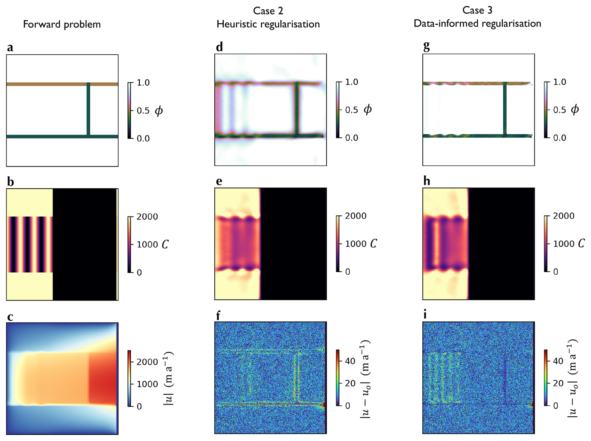
Figure 2 Synthetic experiments showing the model setup (a–c), the results of the inverse problem with heuristic Tikhonov regularisation (d–f) and data-informed regularisation (g–i). (a) prescribed stiffness, (b) prescribed basal friction coefficient, (c) the resulting flow speed, (d) inferred stiffness using heuristic regularisation, (e) inferred basal friction coefficient using heuristic regularisation, (f) misfit of the solution using heuristic regularisation, (g) inferred stiffness using data-informed regularisation, (h) inferred basal friction coefficient using data-informed regularisation, (i) misfit of the solution using data-informed regularisation.

To do this, we set up a domain (Fig. 2a–c) representing an ice stream with damaged shear margins, in which thickness linearly decreases from 512 m on the left hand boundary to 256 m at the calving front on the right. We prescribed periodic regions of low basal stickiness C in the central section to reflect the stripes of hard and soft bed that often underlie real ice streams (Fig. 2b). We defined a stiffness field ϕ of 0.25 in the lower boundary of the ice stream and 0.5 in the upper boundary, indicating asymmetrically softened shear margins, and 0.25 in a vertical stripe on the floating ice, representing a partial thickness crack (Fig. 2a). The resulting flow speed is shown in (Fig. 2c), with flow going from left to right. We considered inverse problems with heuristic regularisation and data-informed regularisation corresponding to cases 2 and 3 as described in Sect. 2.1. For both inverse problems, the input speed data was generated by adding random Gaussian noise to the output of the forward problem (Fig. 2c) with a standard deviation of 10 m a⁻¹. Regularisation strengths were chosen to be optimal according to L-curve analysis. For the data-informed regularisation, values of ξ were chosen to be 0.01 where we prescribed values of ϕ less than 1, and 1 elsewhere.

The solutions confirm that the heuristic regularisation does not prevent the mixing of the two control fields in the grounded region (Fig. 2d–f), and look like it has over-regularised – despite the optimal strength having been chosen according to the L-curve. This is to be expected because the prescribed variations in basal friction in the forward run affect the effective viscosity of the ice, and there is nothing preventing the inverse problem attributing this to stiffness variations. The the data-informed regularisation reduces this degeneracy (Fig. 2g–h), at the expense of a marginally greater misfit (Fig. 2i). The solution for ϕ is, as we would expect, better in the case of data-informed regularisation than heuristic regularisation. This emphasises the important feature of ill-posed problems, namely that there is no simple relationship between the misfit and the quality of the solution. Given the idealised nature of this set up, we take these results as more of a validation of the potential of the method rather than of its real-world efficacy, where our priors are much less well-defined. Specifically, the prior credence in where ϕ≠1 is both high and uniform across the domain in the synthetic example – given that we prescribed it in the forward problem. The next section describes the results of the methods applied to the real case of Pine Island Glacier.

4 Results

4.1 Snapshot inverse problems

We begin with the results of fracture data assimilation applied to a snapshot inverse problem on Pine Island Ice Shelf described in Sect. 2.1. As a reminder, we consider how using the data-informed regularisation alters the problem compared to a case of no regularisation, and the heuristic regularisation of Eq. (4). As in the list shown in Sect. 2.1, we refer to optimisations in which ϕ is unregularised as “case 1”, those in which we apply heuristic Tikhonov regularisation as “case 2” and those in which we apply the data-informed regularisation given by Eq. (8) as “case 3”. We look at the misfits, the output control fields and changes to the problem conditioning. To help interpret the misfits, note that the flow speeds of Pine Island Glacier at the time of these observations ranged from around 1000 m a⁻¹ over the crevasse field on the main grounded trunk of the glacier to around 5000 m a⁻¹ on the central ice shelf.

4.1.1 Softness fields

The ϕ fields in cases 1–3 differ substantively from each other on Pine Island Glacier for this set of geometry and speed data (Fig. 3). This is true for both the grounded and floating ice. Firstly, in both cases 1 and 2 there are large deviations of ϕ from 1 far upstream of the grounding line including substantial softening in the shear margins of even slow-flowing parts of the glacier (Fig. 3a, b). This is completely absent in the solution to case 3 (Fig. 3c). Given the lower misfits in these regions (Fig. 3d, e) compared to case 3 (Fig. 3f), it appears that the model finds it difficult to compensate for the velocity gradients at the margins of the tributary ice streams by enhancing gradients in C where it is encouraged not to alter ϕ. This misfit is, on average, 1.75 and 2.03 m a⁻¹ larger on grounded ice in case 3 than case 1 and 2 respectively (Fig. 4b). In the large fractured region upstream of the grounding line (Fig. 1a, b), the solution for case 3 shows higher amplitude deviations of ϕ from 1 than in cases 1 and 2.

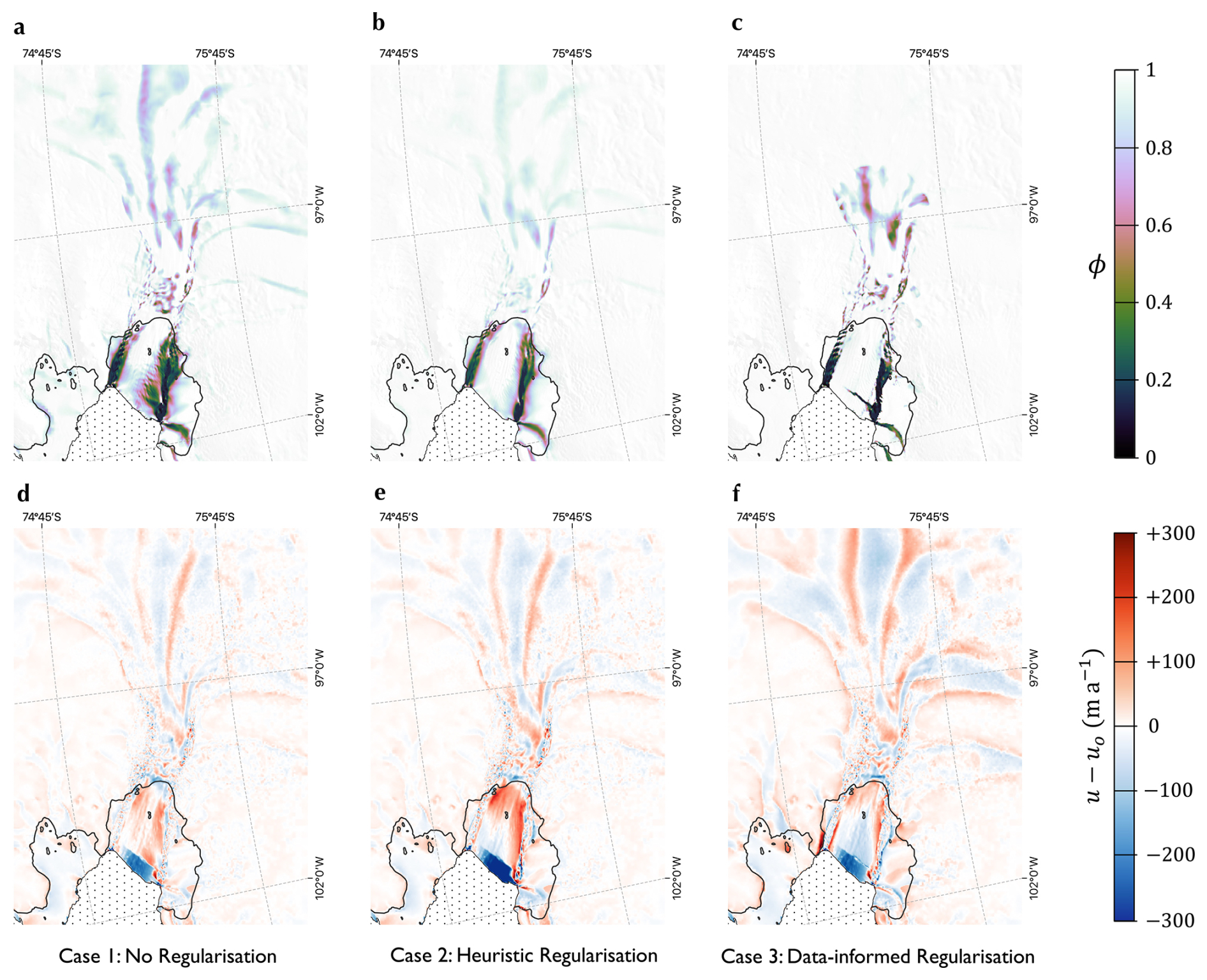
Figure 3 Solutions to the inverse problem with three methods of regularisation. (a–c) Stiffness fields for the unregularised, heuristically regularised and data-informed inverse problems respectively. (d–f) Misfits for the unregularised, heuristically regularised and data-informed inverse problems respectively. Background images are the MODIS Mosaic of Antarctica (Haran et al., 2021), and grounding lines (shown in black) are according to Rignot et al. (2016).

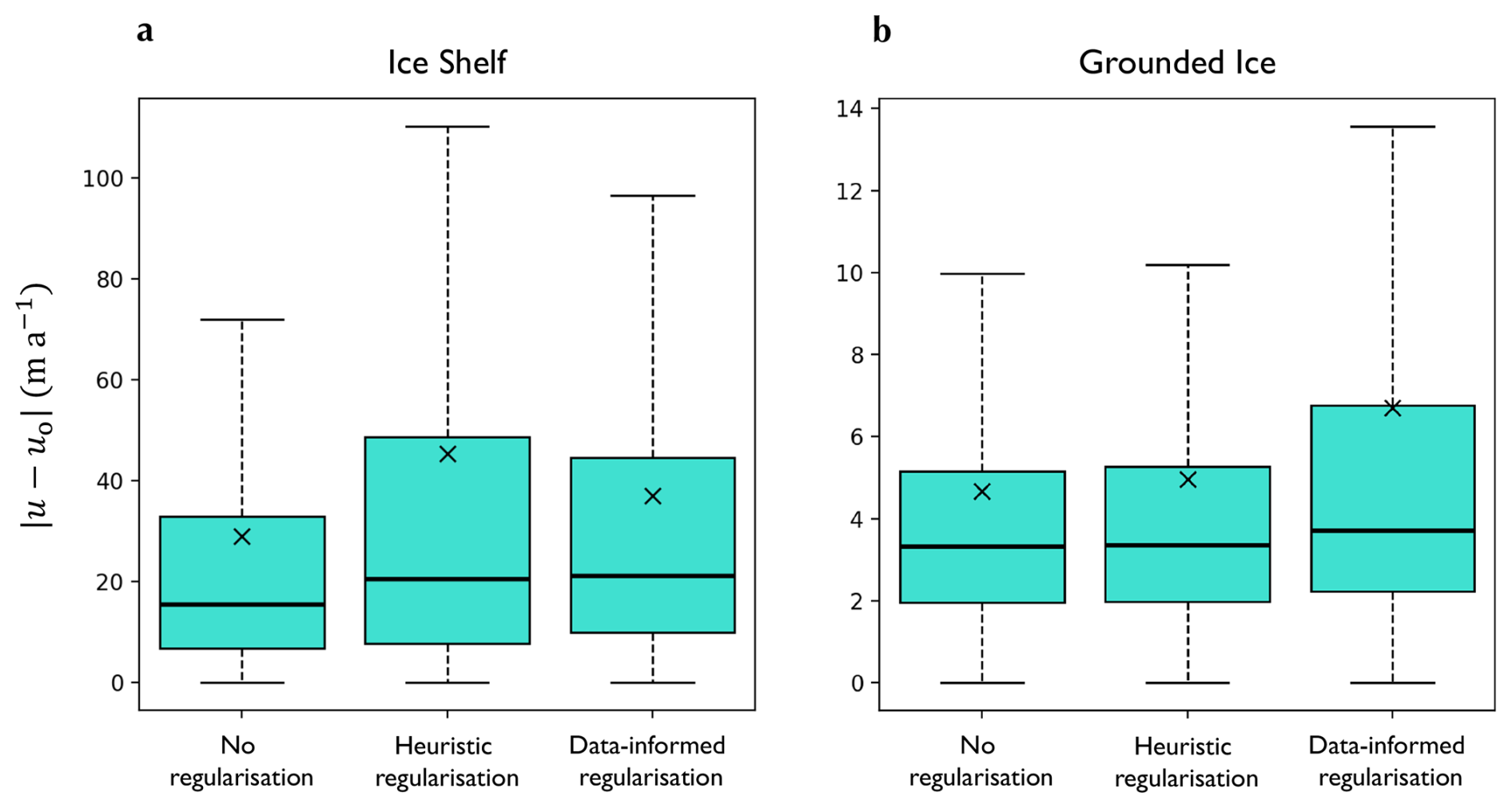
Figure 4 Distributions of misfits for the three regularisation methods for the snapshot inverse problem for floating (a) and grounded (b) ice. Boxes show median and inter-quartile range, whiskers show the 10th and 90th percentiles and crosses show mean values.

The differences in ϕ between the different forms of regularisation are just as pronounced on the floating ice shelf. In cases 1 and 2, softnesses on the ice shelf are smooth and spread to large distances either side of the shear margins. In contrast, in the solution to case 3, softness is concentrated in the shear margin with larger amplitude deviations of ϕ from 1 confined to a smaller area. A portion of the solution degeneracy for ϕ on Pine Island Glacier occurs because the central shelf moves almost entirely by pure advection. In the absence of any significant strain rates, most solutions for ϕ in this region fit the data equally well. The inclusion of an explicit prior appears to help with this by encouraging stiff ice on the central shelf.

The rift that propagated across the ice shelf at the time the speed data was collected caused a discontinuity in the data. The feature is much more clearly resolved in the solution to case 3 than case 2, and even case 1. Hence, it appears difficult for the model to assign low values of ϕ to a region very local to the rift unless encouraged to do so. This is perhaps due to the distributed influence of the ice at the terminus on the dynamics of the ice shelf as a whole (Joughin et al., 2021; Bevan et al., 2023). The idea that a good misfit indicates a good solution is true only for well-conditioned problems, however, it is interesting to note that, on the floating ice, the misfit for case 3 is, on average, 8.38 m a⁻¹ lower than in case 2 (Figs. 3e–f, 4a). The figure also shows that this is largely due to the reduction of the extremal misfits associated with the presence of fractures and associated discontinuities in the speed field.

4.1.2 The effect on problem conditioning

A well conditioned problem damps the contribution of oscillatory, high frequency components of the input data, such as uncorrelated noise in the measured speed, while an ill-conditioned problem is highly sensitive to it. Bringing prior information into the inverse problem has the potential to change the conditioning by enhancing gradients in previously flat regions of the cost landscape. In order to test this change in conditioning, we investigated the impact of perturbations in the input velocity data on the spread of resulting ϕ and u fields.

We performed 10 inverse problems with the addition of uncorrelated Gaussian noise to the input data for the case of data-informed regularisation, heuristic regularisation and no regularisation. Noise was added with a mean of zero and standard deviation of 10 % of the local speed. In each case, we measured the cell-wise standard deviation over the 10 ϕ and u output fields (Fig. 5).

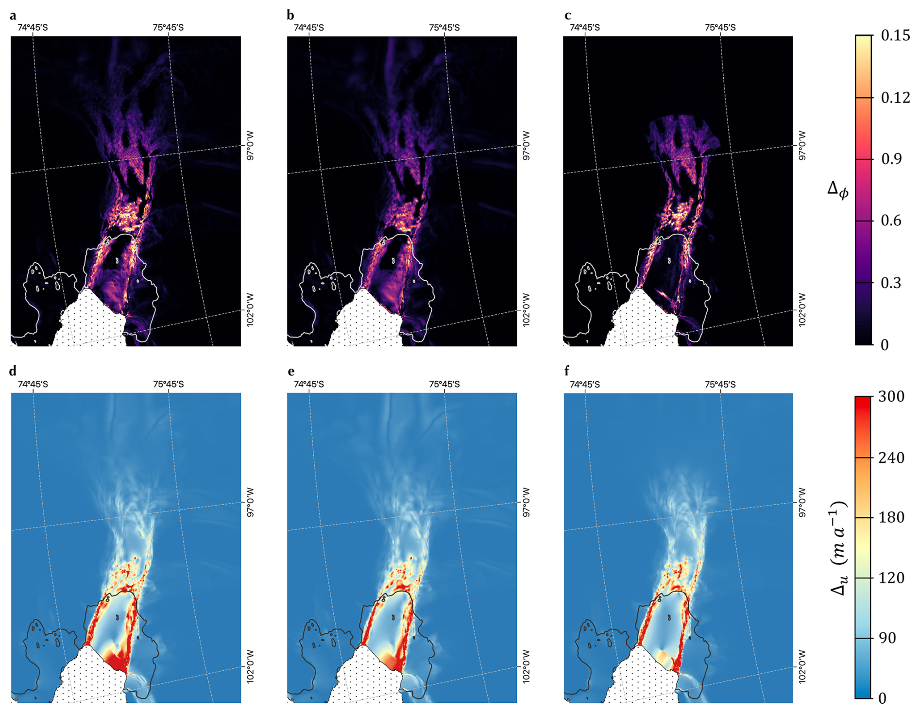
Figure 5 Variation in the solutions for the three methods of regularisation. (a–c) Standard deviation in the softness fields between 10 optimisations with Gaussian noise added to the speed data for the unregularised, heuristically regularised and data-informed inverse problems respectively. (d–f) Associated standard deviations in the modelled speed for the unregularised, heuristically regularised and data-informed inverse problems respectively.

Unsurprisingly, the regularised problems show a smaller spread in the solutions for the control fields – suggesting improved conditioning (Fig. 5a–c). The spread of solutions for ϕ is confined in the case of the data-informed regularisation to the regions of very low ξ, while in those regions, the standard deviations are of similar magnitude to the unregularised case. This is expected because in essence, the data-informed regularisation separates regions in which high-amplitude deviations of ϕ from 1 are penalised (where ξ→1) from regions that are entirely unregularised. The heuristic regularisation, case 2, that is explicitly devised to improve the problem conditioning indeed looks to result in the most well-conditioned problem on grounded ice. However, this is not the case on the central ice shelf, where the degeneracy described above leads to a larger solution variance than in the data-informed case. The spreads of speed (Fig. 5d–f) reflect the spreads of the control fields.

4.2 Inverse problems through time

As listed in Sect. 2.2, we consider two instances of temporal regularisation of the type described in Eq. (9): the “data-informed” case:

$$\begin{array}{}\text{(11)}& \begin{array}{rl}{\mathcal{J}}_{\mathit{\varphi }}& =\underset{\mathrm{\Omega }}{\int }(\mathrm{1}-|f_i-f_{i-\mathrm{1}}\left|\right)\times |{\mathit{\varphi }}_i-{\mathit{\varphi }}_{i-\mathrm{1}}{|}^{\mathrm{2}}\mathrm{d}\mathrm{\Omega }\\ & \text{and}{\mathit{\alpha }}_{\mathit{\varphi }}=\mathrm{0},{\mathit{\alpha }}_t=\mathrm{5}\times {\mathrm{10}}^{\mathrm{6}},\end{array}\end{array}$$

and the “heuristic” case:

$$\begin{array}{}\text{(12)}& \begin{array}{rl}{\mathcal{J}}_{\mathit{\varphi }}& =\underset{\mathrm{\Omega }}{\int }|{\mathit{\varphi }}_i-{\mathit{\varphi }}_{i-\mathrm{1}}{|}^{\mathrm{2}}\mathrm{d}\mathrm{\Omega }\\ & \text{and}{\mathit{\alpha }}_{\mathit{\varphi }}=\mathrm{1.5}\times {\mathrm{10}}^{\mathrm{9}},{\mathit{\alpha }}_t={\mathrm{10}}^{\mathrm{4}},\end{array}\end{array}$$

equivalent to that used in Selley et al. (2021).

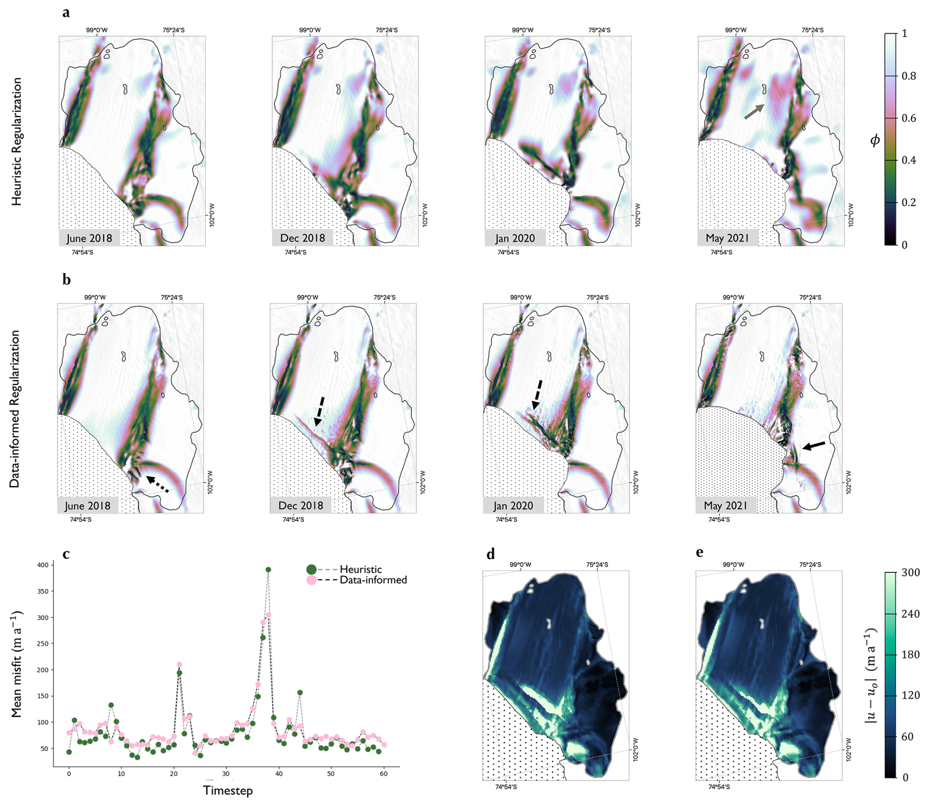
Figure 6 The evolution of the stiffness on Pine Island Ice Shelf between June 2018 and May 2021 for heuristic (a) and data-informed (b) regularisation. (c) Mean misfit over the ice shelf for the two cases through time. (d) Mean misfit over the ice shelf for the heuristically-regularised problem. (e) Timeseries of mean misfit over the ice shelf for the data-informed and heuristically-regularised problems. Background images in (a) and (b) are the MODIS Mosaic of Antarctica (Haran et al., 2021), and grounding lines (shown in black) are according to Rignot et al. (2016).

Using fracture data in successive timesteps to weight the temporal regularisation has a significant effect on the softness fields over the five years of observations compared with the simpler approach (Fig. 6a, b). The data-informed case leads to features of low ϕ which resemble crevasses starting to appear in the southern shear margins after ∼18 months (black dotted arrow Fig. 6b). Rifts that led to the calving of large icebergs in October 2018 and February 2020 are visible as highly linear features of soft ice in the solutions to the data-informed problem (black dashed arrows Fig. 6b). These features are visible in Fig. 6a, though are less easily discernible as rifts. The softness fields in the two cases appear similar by May 2021, with that of the heuristic regularisation looking essentially like a blurred out version of the data-informed case. Both show the southerly migration of the seaward end of the southern shear margin through the time period, and, by 2021, a stripe of soft ice that connects the shear margins of Pine Island and Piglet Ice Shelves. It is only clear in Fig. 6b (black solid arrow) that this stripe of soft ice corresponds to a number of long, parallel rifts. Diffuse blobs of softness can be seen on the central ice shelf in Fig. 6a (May 2021, grey arrow) which are not present in the data-informed case. As the simulation contains no thickness advection and no accumulation rate is specified, it is possible that these could be the result of localised thinning. Otherwise they could once more be the result of ill-posedness. This latter possibility is perhaps more likely given how agnostic the model is to the values of ϕ in the central trunk and that the gravitational forcing is not modified by a change in stiffness.

Throughout the simulation period, the misfits associated with each case are very similar, with generally slightly larger mean misfits over the region in the data-informed case (Fig. 6c, d). The exceptions to this are in the months in which calving events occur – where the misfit is generally elevated as the model struggles to deal with the sudden appearance of large velocity gradients near the glacier terminus. At these times, the data-informed case does slightly better as the observations of rift growth nudge the model towards the right pattern of softening near the terminus.

5 Discussion

The problem of accurately estimating ice softness and basal slip fields from observations of ice speed is dogged by the spector of ill-posedness. In an effort to improve this, we have presented two simple ways of assimilating fracture data (and in one case strain-rate data) into the inverse problem for a marine-terminating ice stream, as a way of providing the problem with prior information. In a number of ways, the effect of these methods, their success and what we learn from the experiments we have carried out differs for grounded and floating ice, so we first review these separately.

5.1 Grounded ice

As discussed above, the presence and evolution of fractures is only a contributing factor in determining ϕ, and the efficacy of the methods aimed at improving snapshot inverse problems depends on the extent to which we apportion softness to fracturing. We have seen in our example of snapshot problems over Pine Island that softness fields on grounded ice found using the data-informed regularisation vary considerably within contiguous areas of observed fracture (Fig. 3c). If fracturing in these regions were truly the main contributor to ice softness, one would expect ϕ to be uniformly less than 1 this region – visually mimicking the uniform coverage of the region by surface fractures (Fig. 1a1). This suggests that here at least, the dominant contribution to our uncertainty in the material properties of the ice softness is not the unaccounted for presence of fractures, but some combination of other factors. This is consistent with the fact that prescribing the data-informed regularisation on the grounded ice dampens the softness away from these regions of fracture but does not change the shape of the solution greatly within them. This suggests that observations of surface fracture on grounded ice have limited use in reducing the degeneracy associated with mixing between C and ϕ fields.

In addition, this constitutes evidence that this kind of grounded surface crevasse has a limited impact on ice dynamics, despite the very low basal frictions we find in this part of Pine Island Glacier (Joughin et al., 2009) and the enhanced membrane stresses required to compensate for this. This is consistent with previous assumptions that the depths of these crevasses is only a small fraction of the ice thickness (Benn and Evans, 2014).

Finally, it is worth noting that the softness fields on grounded ice (and also substantially on floating ice) found using heuristic regularisation (Fig. 3b) mimic many of the features of the strain rate map in Fig. 1c. This suggests greater potential for this data to be used to constrain the softness and that the prior we are currently using doesn't fully capture our assumption that softness should be related to shear (as that of Ranganathan et al., 2021 might, for example). A better prior might, for example, be to assume softness is linear in principal strain rate. Future work should look to investigate different priors that better utilise the strain rate data at our disposal.

5.2 Floating ice

We have shown in both snapshot inverse problems and time-dependent inverse problems that the softness fields over floating ice, resulting from use of our proposed regularisation methods, appear more like what we would expect if the softening were due to fracturing/shearing compared to more heuristic regularisation methods. When encouraged to do so, the model is happy to concentrate softness in regions of observed fracture or high shear without suffering a worse misfit with the prescribed speed data. It is tempting to think that this results in softness fields that appear more likely to accurately represent the material properties of the ice shelf at the time the ice speed data was collected. Unfortunately, the ill-posedness of the problem means that methods of evaluating whether this is true do not extend far beyond a visual assessment of whether the solutions “look right” in the context of our priors, however this is a valuable technique. Though the correlation between rheological parameters, inferred in a manner similar to that described in the heuristic regularisation case here, and crevasse data has previously been shown to be limited (Gerli et al., 2024), we have shown in both the snapshot and time-dependent cases that there are solutions to the inverse problem with at least equally good misfit in which this correlation is undoubtedly strong. Given the many qualitatively dissimilar solutions to the inverse problem, depending on choice of regularisation, e.g. Fig. 3, this seeming contradiction in results is not unexpected, but perhaps warns against over-interpretation of the solutions in both cases.

5.2.1 When would we use these methods?

The example we have chosen for the snapshot inverse problem, where a large rift can be seen on the central trunk of Pine Island Ice Shelf along with an associated discontinuity in u_o, is somewhat contrived to show the differences between the regularisation methods discussed. It is unlikely that a model-user looking to initialise a century-long simulation would choose such data, and would do better to choose data from a time more representative of a typical state of the glacier. Even if a typical state does include fractures and speed discontinuities, without a method of sensibly evolving the softness field through time, it would be reasonable to initialise a model with a smoother solution for (C,ϕ) that might be less representative of the true initial state, but also less specific to it. Hence, softness fields found with the use of fracture data and regularisation procedures we propose here are more likely to be useful in diagnostic simulations, or transient simulations with timescales on the order of years.

A major motivation for investigating these methods of constraining the inverse problem is that the time-varying solutions have potential use in evaluating models that take a continuum damage mechanics approach to parameterising the effect of fractures on large-scale ice rheology (e.g. Sun et al., 2017). In particular, the softness fields shown in Fig. 6b could be used to constrain the way in which a scalar damage field, that acts isotropically on the rheology, is evolved by such a model (Borstad et al., 2016).

5.3 A note on L-curves

Figure 7 shows, on a logarithmic scale, solution and misfit norms at convergence for a number of possible regularisation parameters α_ϕ for Eq. (8), known as an L-curve (Hansen and O'Leary, 1993). Intuition suggests that one should choose the regularisation parameter at the corner of the L-curve, which balances the regularisation and misfit components of the cost function. This can be shown in some circumstances to be the point at which contributions to the solution are balanced between errors in the data and errors in the regularisation (Hansen, 2000). In our case, for the snapshot inverse problems with data-informed regularisation, this is ${\mathit{\alpha }}_{\mathit{\varphi }}\approx \mathrm{5}\times {\mathrm{10}}^{\mathrm{8}}$. However, this choice of parameter results in solutions with fewer crevasse features than we expect to see – such as the rift near the ice shelf terminus (Fig. 6b). Hence, in practise, we choose a parameter an order of magnitude smaller, where we are satisfied with the misfit (staying on the “vertical branch” of the L-curve) but can see some of the detail we believe should be present in the softness field. Though very useful, L-curve analysis can be a blunt instrument and should always be used alongside other heuristics such as visual assessment of the control fields in deciding the regularisation parameter. Its use is based on the assertion that the preferred solution to an inverse problem is one that contains the least extraneous structure (Wolovick et al., 2023). However, for structure to be deemed extraneous, a cost function that encodes a good deal of your prior knowledge is required, which is not often available. This tendency for L-curve analysis to produce over-regularised solutions has been noted previously (e.g. Chamorro-Servent et al., 2019; Milovic et al., 2021), and notably in Recinos et al. (2023).

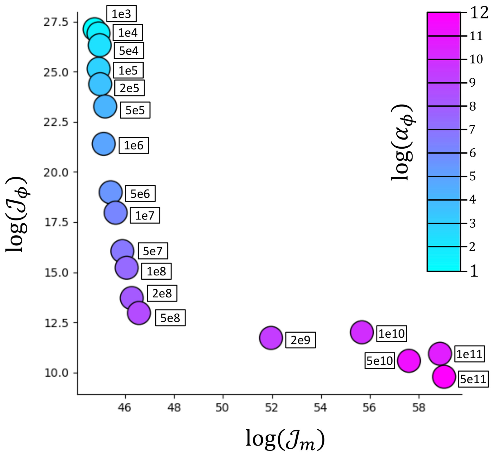
Figure 7 L-curve for the data-informed regularisation. Solution norm (y) and misfit (x) are plotted on a logarithmic scale for different choices of the regularisation parameter α_ϕ.

5.4 Next steps

This article is relatively light on quantitative metrics regarding the success of the proposed methods and future work could aim to change this. In general, the success of a method is difficult to quantify without having a set of experiments for which the right answer is know a priori. We chose to look at real-world data for which this is not the case. We have looked at some quantitative results on the stability of the solutions under noise in the input data (Sect. 4.1.2) and the misfits achieved by different approaches (Sect. 4.1.1, 4.2) but we cannot push these too far. As mentioned above, for ill-conditioned problems such as inverse problems involving viscous flow, there are no guarantees that the quality of the misfit reflects the quality of the solution, so we cannot rely on it (or similar metrics) to differentiate between methods. As such, we have opted largely for qualitative discussion about whether the solutions reflect expected patterns, which we deem more appropriate.

An approach one could take might be to expand on the kinds of methods employed in Sect. 3 and use synthetic data generated from known solutions. For example, assuming crevasse depths for a known crevasse pattern and computing speed given some assumed relationship between crevasse depth and softness. In reality, a range of cases and assumptions should be investigated. The difficulty here is in generalising the results of such experiments to the real-world case, due to the large number of assumptions of unknown validity one would have to make along the way. For example, the methods by which you generate a crevasse pattern, the crevasses you choose to have an effect on the softness, the contributions to the softness do you take to be from sources other than crevasses, the choice of an isotropic softness field in generating the synthetic speed data, etc. However, should others think of methods for quantifying the effects of these assumptions, they would also open up the possibility of properly quantifying the effect of different priors on the solutions of the inverse problem. Of course, this becomes easier the better we can model the different processes that contribute to the softness field; this should continue to be a focus of work in the ice sheet modelling community.

6 Conclusions

We have introduced two ways in which fracture location data, and in one case strain rate data, can be used as prior information to inform the estimation of basal slip and ice softness fields from observations of ice speed. Applications of these methods to snapshot and time-dependent inverse problems over Pine Island Glacier show that little is gained in their use compared to the use of popular heuristic regularisation methods when considering the solutions on grounded ice. This suggests that a failure to account for the presence of fracturing does not dominate our uncertainties in the material properties of grounded ice. This is not true, however, on floating ice, where we see the resolution of fracture features in the static and time-varying softness fields without impacting the misfit, and a reduction in solution degeneracy in regions of low strain rates. This suggests that such methods can be used to provide us with softness fields that better represent the true material properties of the ice shelf at the time of the acquisition of the ice speed data. Such softness fields have potential use in diagnostic modelling, and in constraining models seeking to evolve softness fields in time.