IceAnatomy: a benchmark dataset and methodology for automatic ice boundary extraction from radio-echo sounding data

The measurement of ice thickness is of great importance for the accurate estimation of glacier volume and the delineation of bedrock topography. In particular, this is a crucial factor in forecasting the future evolution of glaciers in the context of a changing climate. In order to derive the ice thickness, the travel time of electromagnetic waves in radargrams acquired by radio-echo sounding (RES) systems is analyzed. This can only be achieved by identifying the ice surface and underlying ice bottom in corresponding radargrams. Manually identifying these two reflection horizons in RES data is a laborious and time-consuming process. Consequently, scientists are attempting to automate this task through the use of techniques such as deep learning. Such automation can significantly reduce the time between a field campaign and the calculation of the glacier's ice thickness distribution. In this paper, we present the first benchmark dataset for delineating the ice surface and bottom boundaries in RES data to facilitate standardized comparisons of deep learning models in the future. The “IceAnatomy” dataset comprises radargrams and the corresponding manual picks, amounting to a total of over 45 000 km of observations. The RES data originate from three sources: FAU (Friedrich-Alexander-Universität Erlangen-Nürnberg, Institute of Geography), CReSIS (Center for Remote Sensing and Integrated Systems), and AWI (Alfred Wegener Institute, Helmholtz Centre for Polar and Marine Research). The dataset comprises different RES systems as well as different pre-processing methods. In addition, the data were acquired over a large range of geographical and glaciological settings, featuring different thermal regimes present in Antarctica and the Southern Patagonian Ice Field. This diversity ensures that the models' behaviors can be analyzed in different scenarios. We define a standardized train–test split for each source in the dataset. This allows us to introduce not only a baseline model trained on the entire training set (the “omni”-model), but also three source-specific baseline models. The source-specific models are trained exclusively on the subset of the training data acquired by the specified source. The baseline models provide an initial benchmark against which subsequent models can be compared. The source-specific models demonstrate more accurate results than the omni-model. For the FAU, CReSIS, and AWI test sets, the source-specific models achieve mean meter errors of 2.1, 23.1, and 4.9 m for the ice surface and 9.1, 78.2, and 29.3 m for the ice bottom. In relation to the mean measured ice thickness of the test set, these errors equate to 1.2 %, 3.1 %, and 0.3 % for the ice surface and 4.9 %, 10.4 %, and 1.5 % for the ice bottom. The dataset and implementation are available at https://doi.org/10.5281/zenodo.14036897 (Dreier et al., 2024) and https://doi.org/10.5281/zenodo.14038570 (Dreier, 2024).

1 Introduction

Glaciers and ice shelves are key indicators of global climate (Haeberli et al., 2007; IPCC, 2013). Knowing their volume and ice thickness distribution is crucial for assessing future cryospheric contributions to sea level rise. Moreover, data on the ice volume of glaciers and ice sheets are necessary for understanding their response to climate change. Ice thickness measurements enable the subsequent prediction of the rate and timing of glacier retreat or disappearance using different types of models. This enables the assessment of a glacier's contribution to regional hydrological cycles and its subsequent influence on local to regional scales with associated socioeconomic impacts (Werder et al., 2020; Ayala et al., 2020; Farinotti et al., 2017). Several techniques to determine ice thickness exist, including seismic, gravitational, and magnetic methods, as well as radio-echo sounding (RES) (Bogorodsky et al., 2012; Kohler et al., 1997). While satellite gravimetry allows for a resolution in the range of kilometers, its spatial resolution does not allow for the interpretation of detailed subglacial features (Willen et al., 2024). Seismic measurements offer a high resolution, but widespread use in the Antarctic region is limited by high exploration costs or logistical infeasibility (An et al., 2023). For this reason, RES is preferred over other methods when an accurate assessment of a subglacial topography is of interest. After pre-processing the RES data, we obtain an image commonly referred to as a radargram. It depicts the cross-section of the glacier along the flight path. Experts can then interpret the RES data by delineating the reflections of surfaces or internal glacial structures. Delineating the ice boundary, defined by the ice surface (air to ice transition) and the ice bottom (ice to ground/water transition), is necessary to obtain the glacier's thickness at each point in the radargram. However, it is a time-intensive task, especially with large datasets (Sime et al., 2011). Several automated and semiautomated approaches to delineate the layers have been developed (Fahnestock et al., 2001; Gifford et al., 2010; Freeman et al., 2010; Rahnemoonfar et al., 2017a, b; Kamangir et al., 2018; Rahnemoonfar et al., 2019; Cai et al., 2020, 2022; Liu-Schiaffini et al., 2022b; Moqadam and Eisen, 2025; Moqadam et al., 2025; Jebeli et al., 2023b). However, these approaches are not comparable as they have been evaluated on different datasets or a different train–test split of the same dataset. In this paper, we present a publicly available, standardized benchmark dataset for ice thickness extraction. It is the first of its kind to be directly designed for deep learning approaches, with a pre-defined train–test split, fully human-annotated ice bottom labels, and different recording systems. It comprises radargrams from Antarctica and Patagonia with polythermal, cold-based, or temperate thermal regimes. The dataset is intended for supervised training and evaluation of deep learning models. Therefore, the dataset includes depth labels for both the ice bottom and ice surface layer. Together with the dataset, we present a baseline model that delineates the ice boundary in a given radargram. The model is based on the U-Net architecture (Ronneberger et al., 2015) and serves as a reference and a starting point for future improvements. In the following, we highlight two potential areas where our algorithm could be further extended to impact real-world scenarios in the future. First, once trained, our algorithm can be executed on virtually any modern laptop in the field. Combined with a pre-processing chain tailored to our approach, this allows for near-real-time analysis of acquired data on-site. Since flight hours are costly and often limited by weather conditions, optimizing their use is crucial. If data can be processed in the field – e.g., between two flights – flight plans could be dynamically adjusted to focus on areas of high interest within the same campaign, e.g., a bedrock ridge beneath a glacier whose extent is greater than initially assumed or ice inflow from large tributary glaciers into the main valley, which alters the bedrock topography at points of conflux more than expected. Second, and perhaps more importantly, the presented method can be further developed to handle more specialized tasks, such as delineating intraglacial water channel systems or identifying water tables within existing datasets. This would represent a step toward a comprehensive, quantitative, and standardized approach for interpreting the ice surface and ice bottom in radagrams, ultimately leading to fully automated products that could significantly benefit the cryospheric research community. In particular, the automated mapping of internal reflection layers remains a critical knowledge gap – one that deep learning is well-positioned to address (Moqadam and Eisen, 2025).

In summary, our contributions are as follows:

1. A novel benchmark dataset, IceAnatomy, for deep-learning-based extraction of ice boundary from RES data is created.

2. A baseline deep learning model for the automatic delineation of the ice bottom and the ice surface is proposed.

3. A thorough evaluation of individual models and an omni-model is conducted on the dataset.

The work is structured as follows: Sect. 2 provides an overview of datasets and algorithms previously used for automatic ice boundary extraction. Subsequently, Sect. 3 gives insight into the recording and processing of the dataset as well as relevant geographical and glaciological factors of the study sites. The baseline models are introduced in Sect. 4. An extensive evaluation of the baseline models and the benchmark dataset is presented in Sect. 5. Lastly, we summarize our research and draw conclusions in Sect. 6.

2 Related works

Over the past decades, RES has been widely used in glaciology. A multitude of publications cover the extraction of ice boundary layers from RES data. In this section, we highlight related RES datasets and layer extraction approaches.

2.1 Datasets

Numerous RES datasets on glaciers and ice sheets are publicly available. However, most existing datasets do not meet the requirements necessary for benchmarking models. Common issues include the fact that most datasets are missing either the layer labels or radargrams or are not publicly available (Young et al., 2021; Blankenship et al., 2018; Dong et al., 2022; Corr, 2020). As a result, accurately benchmarking models to extract the ice bottom often becomes unfeasible. From the datasets, where both the labels and the radargrams are publicly available, a large portion contains labels that are generated automatically with human supervision (Corr et al., 2021; CReSIS, 2025). While this technique is sufficient for clearly visible layers like the ice surface, the ice bottom is often too ambiguous for an automatic tracker to capture accurately in its entirety. Thus, the supervising human would have to intervene in such cases. However, the level of human involvement and the methods to validate the picking process are rarely specified, creating a level of uncertainty that undermines the reliability of the benchmark dataset. Lastly, some datasets also do not satisfy the qualitative standards. While the picking process can often be subjective, errors like a negative ice thickness are an indication of a lack of accuracy, making them unsuitable for training or evaluating deep learning approaches (CReSIS, 2012, 2013). Since listing and evaluating every dataset is virtually impossible, we focus our comparison on datasets that have been used to extract the ice boundary in previously published work and for which both radargrams and human-annotated labels are publicly available. These constraints significantly limit the number of related datasets.

The one RES system that has been used extensively to collect such data is the Multichannel Coherent Radar Depth Sounder versions 1–5 (MCoRDS) (Allen et al., 2012a), which was used, for example, in NASA's Operation IceBridge (OIB) program on a McDonnell Douglas DC-8-72 jetliner (Shi et al., 2010a). The data acquired over Antarctica in 2009 are the most widely used (Crandall et al., 2012; Lee et al., 2014; Rahnemoonfar et al., 2017a, b; Berger et al., 2018; Kamangir et al., 2018). However, data from different years (Kamangir et al., 2018; Mitchell et al., 2013; Cai et al., 2020; García et al., 2021a, b; Cai et al., 2022, 2019; Ghosh and Bovolo, 2022; García et al., 2023; Donini et al., 2022; Ilisei and Bruzzone, 2014, 2015) and other locations like Greenland (Donini et al., 2022) and the Canadian Arctic Archipelago (Xu et al., 2017, 2018) were also analyzed.

Only very few publications included data from RES systems other than MCoRDS. Gifford et al. (2010) extracted the ice boundary from data acquired by a predecessor RES system (Lohoefener, 2006) during 2006 and 2007 in Greenland. Dong et al. (2022) featured data from the Chinese Academy of Sciences' Deep Ice Radar acquired during the 29th Chinese Antarctic Scientific Expedition. Lastly, Liu-Schiaffini et al. (2022a) used algorithm-assisted human-labeled data acquired in the Canadian Arctic and Antarctica by the University of Texas Institute for Geophysics' high-capability radar sounder (HiCARS). A major downside of these datasets is that they do not provide standardized training and evaluation splits, making inter-model comparison challenging. Furthermore, datasets usually only focus on a single area, e.g., Greenland or Antarctica, which makes generalization to other areas or glaciological settings difficult to verify. IceAnatomy addresses this issue by including data from multiple study sites, radar systems, and glaciological settings. It also provides standardized splits for training and evaluation to allow for an accurate and fair comparison between models. In conclusion, to the best of our knowledge, there is no comparable benchmark dataset for ice boundary extraction from radio-echo sounding data.

2.2 Algorithms

RES has been employed to detect crevasses (Liu et al., 2020; Walker and Ray, 2019; Williams et al., 2012, 2014) and the ice boundary (Crandall et al., 2012; Lee et al., 2014; Rahnemoonfar et al., 2017a, b; Berger et al., 2018; Kamangir et al., 2018; Mitchell et al., 2013; Xu et al., 2017, 2018; Cai et al., 2022; Gifford et al., 2010; Dong et al., 2022; Liu-Schiaffini et al., 2022a), to segment subsurface structures (Cai et al., 2020, 2019; García et al., 2021a, b; Ghosh and Bovolo, 2022; García et al., 2023; Donini et al., 2022; Ilisei and Bruzzone, 2014, 2015), and to track internal ice and snow layers (Crandall et al., 2012; Karlsson et al., 2013; Ibikunle et al., 2020; Rahnemoonfar et al., 2021; Varshney et al., 2020, 2021; Yari et al., 2019, 2020; Dong et al., 2022). Moqadam and Eisen (Moqadam and Eisen, 2025) provide an overview of the methods used in this domain.

To obtain the ice boundary, one can either directly delineate the ice surface and bottom or first segment different regions such as ice, bedrock, and air and then extract the two layers during post-processing. Most existing studies (Crandall et al., 2012; Lee et al., 2014; Rahnemoonfar et al., 2017a, b; Berger et al., 2018; Kamangir et al., 2018; Mitchell et al., 2013; Xu et al., 2017, 2018; Cai et al., 2022; Gifford et al., 2010; Dong et al., 2022; Liu-Schiaffini et al., 2022a) prefer direct extraction. Fewer studies (Cai et al., 2020, 2019; García et al., 2021a, b; Ghosh and Bovolo, 2022; García et al., 2023; Donini et al., 2022; Ilisei and Bruzzone, 2014, 2015) use the segmentation approach. The segmentation approach assigns a semantic class to each pixel in the radargram, from which the ice boundaries can be derived directly or after post-processing.

In terms of methodology, early studies mainly used classical image processing and machine learning techniques such as hidden Markov models (Crandall et al., 2012; Berger et al., 2018), Markov chain Monte Carlo (Lee et al., 2014), contour detection (Rahnemoonfar et al., 2017a), the level set approach (Rahnemoonfar et al., 2017b; Mitchell et al., 2013), Markov random fields (Xu et al., 2017), edge-based and active contour methods (Gifford et al., 2010), Kullback–Leibler maps (Ilisei and Bruzzone, 2014), and support vector machines (Ilisei and Bruzzone, 2015). After 2017, studies turned to convolutional neural networks (CNNs) (Kamangir et al., 2018; Cai et al., 2020, 2019; García et al., 2021a; Cai et al., 2022; Donini et al., 2022; Dong et al., 2022; Liu-Schiaffini et al., 2022a; García et al., 2021b, 2023; Jebeli et al., 2023a, b; Matsuoka et al., 2021; Moqadam et al., 2025), combinations of CNNs and recurrent neural networks (RNNs) (Xu et al., 2018), and combinations of CNNs and transformers (Ghosh and Bovolo, 2022).

In comparison, we rely on the U-Net architecture from (Ronneberger et al., 2015) to evaluate our newly created dataset. Furthermore, we integrate Atrous Spatial Pyramid Pooling from Chen et al. (2018) and the ResBlock design from Esser et al. (2020) to improve the performance.

3 Dataset

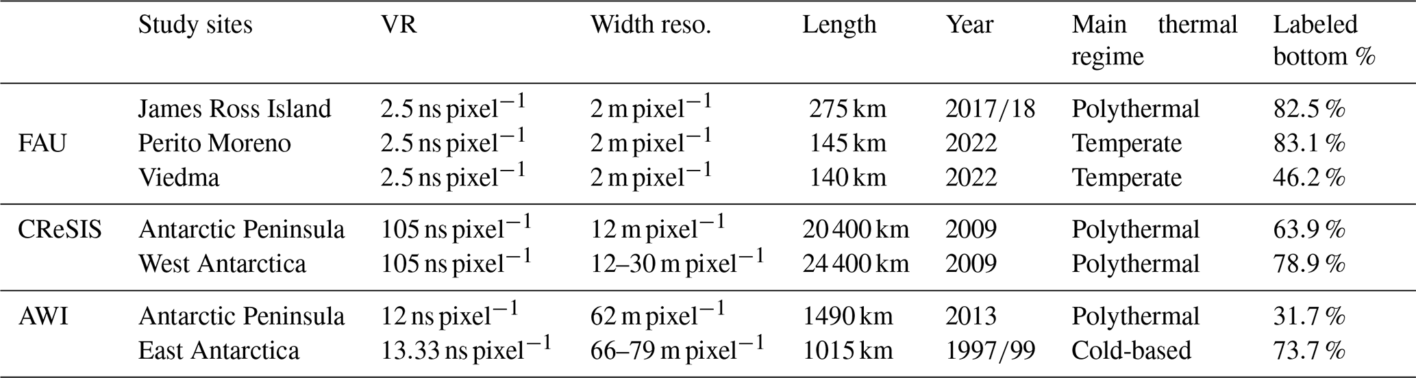
In this section, we introduce the benchmark dataset “IceAnatomy”, which covers several different geolocations and was acquired by multiple radar systems. We divide the dataset into three subsets based on the sources of the data: the AWI (Alfred Wegener Institute, Helmholtz Centre for Polar and Marine Research), CReSIS (Center for Remote Sensing and Integrated Systems), and FAU (Friedrich-Alexander-Universität Erlangen-Nürnberg, Institute of Geography) subsets. A summary of the most important information about the dataset is given in Table 1.

Table 1 A summary of details about the IceAnatomy benchmark dataset (Lippl et al., 2019; Shi et al., 2010b; Rückamp and Blindow, 2012; CReSIS, 2024a; Allen et al., 2012b; Steinhage, 2001, 2015). VR stands for the vertical resolution of the two-way travel.

3.1 Study sites

3.1.1 Southern Patagonian Ice Field

The Southern Patagonian Ice Field (SPI) is the largest temperate ice body in the Southern Hemisphere. It is characterized by one of the highest mass loss rates in the world (Zemp et al., 2019; Marzeion et al., 2018; Hugonnet et al., 2021) and by its large outlet glaciers that drain into lakes or the ocean (Aniya, 1999). Two of the largest eastward-flowing outlet glaciers in the region are the Perito Moreno and Viedma glaciers. The only way to obtain information over large areas about their bedrock topography is by helicopter-borne RES measurements. This is particularly applicable to the lower parts of the glaciers, which are surrounded by steep mountain flanks and have heavily crevassed surfaces. As the glaciers are temperate, i.e., most of the ice is close to or at the pressure melting point, they contain a relatively high proportion of water (Aristarain and Delmas, 1993; Millan et al., 2019; Strelin et al., 2014; Schaefer et al., 2015). This characteristic, combined with the steep and deep glacier troughs, often makes analyzing radargrams challenging. Hence, we hypothesize that they pose a significant challenge to machine learning systems. Figure 1 shows the location of both glaciers on the east of the SPI.

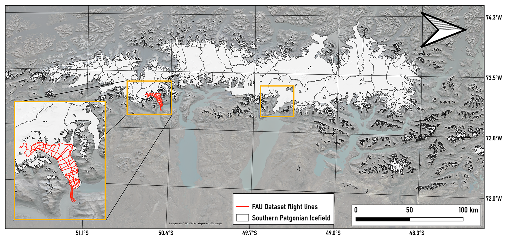
Figure 1 Overview of the Southern Patagonian Ice Field (inland). Orange boxes indicate surveyed areas of Perito Moreno Glacier and Viedma Glacier. Black lines indicate flight paths over the Perito Moreno Glacier. The background is a hillshaded SRTM; © 2025 NASA, map data © 2025 Google Earth optical imagery (RGI 7.0 Consortium, 2017). Maps are rotated by 90°.

3.1.2 Antarctica

As depicted in Fig. 2, the IceAnatomy dataset offers three major study sites in Antarctica: the Antarctic Peninsula (including James Ross Island, JRI), West Antarctica, and East Antarctica.

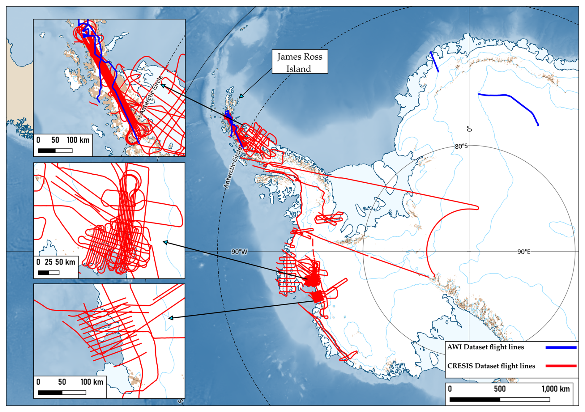
Figure 2 Flight paths of the AWI and CReSIS campaigns in Antarctica. The background is assembled with help from the Quantarctica QGIS project (Matsuoka et al., 2021).

The Antarctic Peninsula is the most represented region in the benchmark dataset, as it is present in all three RES subsets. It exhibits one of the milder climates in Antarctica, with an annual average temperature of −3.2 °C (Morris and Vaughan, 1994). This is also reflected in the thermal regimes present in the region, as it contains temperate, cold-based, and polythermal ice. The temperate portions of the Antarctic Peninsula are frequently near the margins and at lower elevations, while the cold-based ice regions are generally found at higher elevations. The transition zones between higher and lower elevations commonly contain polythermal ice (Van Liefferinge and Pattyn, 2013; Macelloni et al., 2019). However, elevation alone is often not sufficient to determine the thermal regime. A comparison with the ice velocity maps of Rignot et al. (2011) and Gardner et al. (2022) reveals that fast-moving ice is present even in higher-elevation areas, which is atypical for cold-based areas (Park et al., 2024; Dawson et al., 2022). This suggests that there is a significant amount of polythermal ice at higher elevations and that the main thermal regime is polythermal. Another significant characteristic of the Antarctic Peninsula is its relatively shallow ice sheet compared to the rest of Antarctica. On average, the ice sheet is estimated to be 610 m thick inland and 300 m in the ice shelves (Drewry et al., 1982). This results in a generally clearer signal because the signal has to travel through less ice and is less likely to be distorted by impurities in the glacier.

West Antarctica is significantly colder than the Antarctic Peninsula, with an annual average temperature of approximately −28.1 °C and a primarily polythermal thermal regime (Morris and Vaughan, 1994). Polythermal regions only commonly occur at the margins and the coastline, while cold-based zones are mainly present at higher elevations (Macelloni et al., 2019; Van Liefferinge and Pattyn, 2013; Rignot et al., 2011). West Antarctica also contains relatively thick ice with inland ice sheets estimated to be 1780 m thick and ice shelves around 375 m (Drewry et al., 1982).

The last subregion in Antarctica is East Antarctica. It exhibits the coldest climate of the three areas, with an annual average temperature of around −59.8 °C and a primarily cold-based thermal regime (Morris and Vaughan, 1994). Temperate areas are commonly found near the margins, while polythermal zones act as a transitional zone between the cold-based and temperate areas (Macelloni et al., 2019; Van Liefferinge and Pattyn, 2013; Rignot et al., 2011). East Antarctica is also the region with the generally thickest ice. On average, its ice sheets are approximately 2630 m thick inland and 400 m in its ice shelves (Drewry et al., 1982).

3.2 Dataset generation

3.2.1 FAU data

The RES system of FAU is a broadband 25 MHz bistatic monopulse sounder designed as a sling load for helicopter use. It is a functional replica of the BGR-P30 system (Blindow et al., 2012). The antenna weighs roughly 280 kg and can be attached to any helicopter type that allows for the attachment of a sling load and has the required take-off capacity. The system is typically operated 20 m above ground at a nominal airspeed of 60 km h⁻¹.

The radar time series are collected at a 2.5 ns sampling rate using 256-fold stacking to improve sensitivity and signal-to-noise ratio. The traces are collected at a rate of 10 Hz, corresponding to approximately a 2 m spatial sampling rate. The data are georeferenced by two Leica GS16 multifrequency Global Navigation Satellite System (GNSS) systems. The rover antenna is mounted on the radar antenna in a central position, while the base station is installed in proximity to the landing and starting area. After differential processing of the GNSS data, the positions are matched to the radar traces before further processing is applied. Then, the RES data are processed in REFLEX v8.5 software, developed by Sandmeier Geophysical Research. The processing flow comprises the following steps and is applied to subsections of each flight: equidistant trace interpolation, shift for time zero, subtracting special average, bandpass filter, amplitude regulation by gain function (cold ice) or energy decay (temperate ice), 2D migration, and static correction. To apply the 2D migration, it is necessary to derive a velocity model comprising an air and an ice layer. For the air layer, the wave travels at the speed of light, while for the ice layer, we assumed a speed of 0.168 m ns⁻¹ (Johari and Charette, 1975). Especially in temperate ice, the migration helps to focus the scattered energy to enhance the ice bottom reflections.

The RES data for JRI were acquired during two different airborne ground-penetrating radar campaigns in 2017 and 2018 (Lippl et al., 2019). Since Gourdon Glacier consists mainly of bare ice, no firn correction was applied for the outer parts of the profile. For the data on the plateau, a standard correction for firn and snow (+10 m, AWI/BAS Bedmap 1 mission summary) as used in the British–Argentinian survey was assumed (Lythe and Vaughan, 2001). The RES data for Perito Moreno Glacier and Viedma Glacier were acquired in March and April 2022. For these study sites in the FAU subset, the ice is thicker than the radar's maximum penetration depth of estimated 700 m (Blindow et al., 2011). The original depth of the radargrams is over 6000 pixels, which equates to over 1300 m on average – the total depth in meters is not constant due to fluctuations in the flight height of the helicopter. We cut the radargrams to 4096 pixels, which corresponds to an average of about 800 m. This saves computing power while keeping all the essential information. To restore the full flight traces in the FAU dataset from their subsampled parts, we reassembled the radargrams according to their trace numbers. Any conflicting depths for the ice surface and bottom in overlapping parts were smoothened with Gaussian importance weighting. Furthermore, in rare cases, the initially labeled ice surface and bottom had small gaps. To avoid such inconsistencies, we filled gaps of 11 pixels or fewer in the ice surface and bottom via bicubic interpolation using the two nearest manually labeled points as a reference.

The initial layer labels were fully manually annotated by a single interpreter to ensure consistency throughout the dataset. Surface reflections were generally straightforward to identify; however, in heavily crevassed areas, we increased the resolution to delineate the air–ice interface as accurately as possible across these features. Bedrock picks were conducted using the same approach. In regions with ambiguous reflections, ReflexW (Sandmeier, 2024) software enabled zooming into specific subsets of the radargrams, thereby enhancing the clarity of features of interest. Additionally, several intersecting profile lines provided cross-points for internal validation. These intersections were annotated independently by the same interpreter and subsequently compared. All cross-profile values fell within the expected margin of error, even in areas with steep slopes or greater depths (i.e., deviations < 10 %). At Perito Moreno Glacier, two control points from previous studies were available for comparison (Sugiyama et al., 2011; Stuefer et al., 2007). The first, along the “Buscaini” profile, corresponds to a seismic survey conducted in 1996, which reported a maximum ice thickness of 720 m. The second, located nearer to the glacier terminus, corresponds to a borehole drilled in 2010, revealing an ice thickness of 515±5 m. Both control points were in close agreement with our ice thickness estimates.

3.2.2 CReSIS data

The CReSIS data were recorded during the 2009 campaign of Operation Ice Bridge in Antarctica, which comprised 21 missions. Three were sea ice surveys and thus are not included in the CReSIS dataset. The remaining 18 missions can be split into two groups: six missions focusing on the Antarctic Peninsula (PEN1, PEN2, PEN3, PEN4, PEN5, and LVISPEN) and 12 missions exploring West Antarctica (PIG1, PIG2, PIG3, PIG4, LVISPIG, LVIS86, GETZ1, ABBOTT1, TSK1, TSK2, TSK3, and TSK4) (Allen et al., 2012b). All 18 missions employed the Multichannel Coherent Radar Depth Sounder (MCoRDS) flown on a McDonnell Douglas DC-8-72. It has a center frequency of 195 MHz and an eight-channel chirp signal to accurately assess the ice (Rodriguez-Morales et al., 2014; Shi et al., 2010b).

To process the recorded data, the standard CReSIS L1B CSARP-mvdr (minimum variance distortionless response) processing steps were applied. These include pulse compression via a Tukey and Hanning window, beam forming, motion compensation, synthetic aperture radar processing in combination with f–k migration, channel combination, and waveform combination (CReSIS, 2024b). After the processing, the radargrams had a vertical resolution of the two-way travel time (vertical resolution, VR) of 105 ns pixel⁻¹ and a width resolution of 12–30 m pixel⁻¹ depending on the mission.

We obtained the fully processed CReSIS subset by downloading the CSARP-mvdr processed L1B product from the CReSIS website and taking the square root of the amplitudes. Likewise, CReSIS also provides downloads for the annotated ice bottom and surface layers on their website (CReSIS, 2024a). According to Lee et al. (2014) and Crandall et al. (2012), the ice bottom surface is human-annotated but noisy. Although the noise might pose a problem for certain approaches, we chose not to alter the labels. The reason for this is that the dataset has been used previously in other publications, and in order to remain comparable, we use the same labels. However, to provide additional context regarding the quality, CReSIS provides a quality label for every pick. The label indicates the annotator's confidence, ranging from 1 (high) to 3 (low). We include these labels in the benchmark dataset for future research. The general picking procedure for CReSIS data is outlined in CReSIS (2024b).

3.2.3 AWI data

The AWI subset was recorded during campaigns in Dronning Maud Land in 1997 and 1999 (Steinhage et al., 2023b, a) and in the Antarctic Peninsula in November 2013 (Steinhage, 2015). All three campaigns employed a version of the electromagnetic reflection system (EMR) radar system with a center frequency of 150 MHz and the toggle mode enabled. The toggle mode alternates the radar's pulse length between 60 and 600 ns periodically. Thus, the system can achieve a decent VR while capturing deep internal layers of the ice. The processing of the recorded data was similar for all three campaigns. The data were differentiated, rescaled, high-pass-filtered, and bandpass-filtered. To reduce the amount of noise in a radargram, multiple traces were combined into a single trace. In detail, 10 traces were combined for the 1997 and 1999 flights, and seven traces were combined for the 2013 flight (Steinhage, 2001; Nixdorf et al., 1999; Steinhage et al., 2001). Automatic gain control was used to normalize the amplitude values. After the processing, the radargrams had a VR of 12–13.33 ns pixel⁻¹ and a width resolution of 66–79 m pixel⁻¹ depending on the campaign.

The ice surface and ice bottom were annotated by one person. To ensure consistency, plausibility checks were performed at crossing points with other profiles from the same or related campaigns. No systematic biases were observed. In the picks, gaps of 11 pixels or fewer were filled using bicubic interpolation. Finally, for the radargrams from 1997 and 1999, all data below 3600 pixels, which is about 4 km, were discarded because only noise was visible at these depths. The gathered data were processed with FOCUS, DISCO, LANDMARK, and Python.

4 Baseline method

To demonstrate the usability of the dataset, we present a baseline method in this section. The method's pipeline consists of pre-processing steps and a deep learning model, elaborated in the following subsections.

4.1 Pre-processing

The radargrams are given in relative power p to the recorded amplitudes, which we first convert to decibels using the following formula:

$$\begin{array}{}\text{(1)}& \mathrm{dB}=\mathrm{10}\cdot {\log }_{\mathrm{10}}\left(p\right).\end{array}$$

Next, we apply a z-score normalization; i.e., we subtract the mean and divide by the standard deviation. However, the mean and standard deviation are not formed over the entire IceAnatomy dataset because there is a strong divergence in the recorded spectrum values between the different subsets. This divergence is caused by the large difference in radar systems and data processing, which represents a domain shift. Therefore, normalization is performed separately for the AWI and CReSIS data and for the three study sites in the FAU subset.

Then, the normalized radargrams of the entire IceAnatomy dataset are resized to a standard height of 1024 pixels to limit the computational cost and simplify processing. Finally, each radargram is cut into patches with a width of 512 pixels and a total height of 1024 pixels. For trajectories whose width is not divisible by 512, we apply symmetric padding at the end.

4.2 Deep learning model

We apply a deep learning model to extract the ice boundary from the radargram. The model's architecture is depicted in Fig. 3 and is based on the U-Net (Ronneberger et al., 2015), a widely adopted approach for tasks such as ice boundary extraction and comparable tasks (He et al., 2019; Jebeli et al., 2023b, a; Donini et al., 2022; Dong et al., 2022; Ghosh and Bovolo, 2022; Moqadam et al., 2025). While more recent architectures, such as the transformer (Vaswani et al., 2017), may offer better performance, they also come with increased computational costs, larger models, and other practical limitations. The U-Net consists of three components: an encoder, a decoder, and a bottleneck.

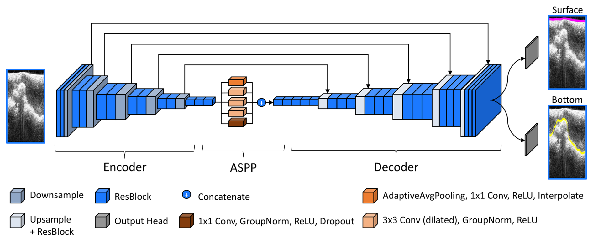
Figure 3 The architecture of the proposed deep learning model. It receives the normalized amplitudes of a radargram as input and predicts the ice surface and the ice bottom as two separate outputs. The Atrous Spatial Pyramid Pooling contains three dilated convolutional layers, one convolutional layer with adaptive average pooling, and a 1×1 convolutional layer. It utilizes the rectified linear unit (ReLU) activation function, which is defined as $\mathrm{ReLU}\left(x\right)=max(x,\mathrm{0})$.

The encoder extracts features from the radargram into a feature map, the decoder utilizes the feature map to make a prediction, and the bottleneck connects these two components. As the model has to handle large input sizes, the encoder contains five down-sampling steps to process the input, while the decoder has five up-sampling steps to reconstruct the original size. In the encoder, each down-sampling step consists of two residual blocks (ResBlocks), while in the decoder, each up-sampling step consists of three ResBlocks (Esser et al., 2020) (see Appendix B for a detailed summary of its structure). In the bottleneck, we inserted an Atrous Spatial Pyramid Pooling (ASPP) (Chen et al., 2018) layer. ASPP processes the same feature map in parallel with differently dilated convolutional layers. In contrast to typical convolutional layers, dilated convolutional layers do not utilize a set of adjacent pixels. Instead, they sample a set of pixels from a grid around a center point, thereby achieving differently sized fields of view. The sampling is uniform and based on a dilation rate. The chosen dilation rates in this model are 1, 4, and 6. Since the model is based on the U-Net architecture, it also includes skip connections. Skip connections directly forward the output of each down-sample step in the encoder to the corresponding parts in the decoder via concatenation. The increased channel dimensions in the decoder are solved by including an additional ResBlock for channel reduction after each up-sampling step in the decoder.

To calculate the final prediction of the model, we first forward the feature map computed by the U-Net into two separate output heads, each consisting of a single ResBlock. Each output head then creates one probability map, resulting in two final probability maps. The first one represents the probabilistic prediction of the ice surface, while the second one represents the probabilistic prediction of the ice bottom. The final prediction of the model is then the highest probable prediction of each column, which we compute by applying a column-wise argmax operation.

To train the network, we employ a custom loss, a cost function that gives feedback to the network by measuring the difference between the prediction and the corresponding labeled ice boundary. The custom loss consists of two parts: a distance-based (L_dist) loss and a classification (L_class) loss,

$$\begin{array}{}\text{(2)}& L=L_{\text{dist}}+L_{\text{class}}.\end{array}$$

For both the classification and distance-based losses, the probability maps of the ice surface (${\widehat{Y}}_{\text{s}}$) and ice bottom (${\widehat{Y}}_{\text{b}}$) are treated column-wise, i.e., per trace. The classification loss is a smoothed cross-entropy loss (L_CE) where each pixel in a column is treated as a separate class, and the pixel closest to the ground-truth boundary is considered the correct class. The distance-based loss (L_Dist) sums up the probabilities in the column, which are weighted with a distance map. The distance map contains the distance to the correct pick for each pixel. Hence, the further away the predicted pick is from the annotated layer, the greater the loss. Appendix C provides a more in-depth overview of the loss function.

The annotations in the dataset have discontinuities in the labeled layers where the ice bottom dropped below the radar's penetration depth, the receiver flew over the edge of the glacier, or the signal was too ambiguous for experts to interpret. Tracks for which no pick is available for a layer are not included in the loss calculation and the evaluation.

5 Evaluation

5.1 Evaluation metrics

Previous work either directly extracted the ice boundaries or deduced them from an intermediate segmentation, where they predicted a semantic class for every pixel in the radargram. Depending on the chosen method, the metrics used to assess the quality of the predictions differ. For segmentation approaches, most of these metrics are based on a confusion matrix that measures how accurately the model distinguishes between a chosen positive class and all the other classes, dubbed the negative class. A confusion matrix contains four measurements: true positives (TPs) (the number of correctly predicted pixels for the positive class), true negatives (TNs) (the number of correctly predicted pixels for the negative class), false positives (FPs) (the number of wrongly predicted pixels for the positive class), and false negatives (FNs) (the number of wrongly predicted pixels for the negative class). Based on these four measurements, more sophisticated metrics are defined for the segmentation approaches. The most commonly employed one is the accuracy $\left(\frac{\mathrm{TP}+\mathrm{TN}}{\mathrm{TP}+\mathrm{FP}+\mathrm{FN}+\mathrm{TN}}\right)$ (García et al., 2021a, b, 2023; Ghosh and Bovolo, 2022; Donini et al., 2022; Ilisei and Bruzzone, 2015). Less commonly used metrics include the intersection over union (IoU) $\left(\frac{\mathrm{TP}}{\mathrm{TP}+\mathrm{FP}+\mathrm{FN}}\right)$ (Cai et al., 2019), precision $\left(\frac{\mathrm{TP}}{\mathrm{TP}+\mathrm{FP}}\right)$ (Ghosh and Bovolo, 2022), recall $\left(\frac{\mathrm{TP}}{\mathrm{TP}+\mathrm{FN}}\right)$ (Ghosh and Bovolo, 2022), the F₁ score $\left(\mathrm{2}\frac{\mathrm{Precision}\cdot \mathrm{Recall}}{\mathrm{Precision}+\mathrm{Recall}}\right)$ (Cai et al., 2020; Ghosh and Bovolo, 2022), sensitivity $\left(\frac{\mathrm{TP}}{\mathrm{TP}+\mathrm{FN}}\right)$ (García et al., 2023; Donini et al., 2022), specificity $\left(\frac{\mathrm{TN}}{\mathrm{TN}+\mathrm{FP}}\right)$ (García et al., 2023; Donini et al., 2022), and the error rate $\left(\frac{\mathrm{FP}+\mathrm{FN}}{\mathrm{TN}+\mathrm{TP}+\mathrm{FP}+\mathrm{FN}}\right)$ (Ilisei and Bruzzone, 2014).

For direct extraction approaches, the mean column-wise absolute error, also called the mean absolute error (MAE) (Crandall et al., 2012; Lee et al., 2014; Rahnemoonfar et al., 2017a; Berger et al., 2018; Mitchell et al., 2013; Xu et al., 2017, 2018; Gifford et al., 2010; Dong et al., 2022; Liu-Schiaffini et al., 2022a), is the most common metric. It measures the average pixel-wise distance between the annotated layer and the prediction. Other distance-based metrics include the median of the column-wise mean absolute error (Lee et al., 2014; Rahnemoonfar et al., 2017a; Berger et al., 2018; Xu et al., 2017), the mean squared error (MSE) (Crandall et al., 2012; Mitchell et al., 2013; Dong et al., 2022), the root mean square error (RMSE) (Liu-Schiaffini et al., 2022a), and the largest underestimation and overestimation (Gifford et al., 2010). We can also define confusion-matrix-based metrics on the layer extraction task. In that case, we define each height pixel of the radargram as a separate class and the closest pixel in each column to the corresponding layer as the correct class. However, a limitation of confusion-matrix-based metrics, such as precision, is that they do not account for distance weighting. For example, if a prediction is always 1 pixel next to the annotated layer, also known as ground truth (GT), the confusion-matrix-based metrics will have the worst possible value, even though it is a near-perfect prediction. Therefore, some studies (Xu et al., 2017; Gifford et al., 2010; Liu-Schiaffini et al., 2022a) have relaxed these confusion-matrix-based metrics by considering predictions a few pixels from the ground truth to still be correct.

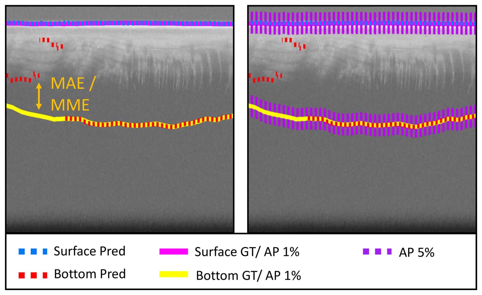
Figure 4 A visual representation of the four metrics used in this work. The left side of the figure depicts the MAE and MME as the difference between prediction and ground truth (GT), respectively. Meanwhile, the right side of the figure features the AP-1 % and AP-5 %, respectively, as an interval around the ground truth. Note that the ground truth and the predictions are technically float numbers. However, we thickened the ground truth by 20 pixels to improve visibility.

As metrics for our benchmark framework, we have chosen the MAE, two relaxed average precision (AP) metrics, and the mean meter error (MME). The MAE is calculated as the column-wise difference in pixels between the ground-truth depth of a layer and the predicted depth. Resizing the radargram will change the value of this metric. Therefore, we also introduce the MME, which approximates the real-world error. We calculate the MME by multiplying the MAE with the product of the wave velocity in the medium and the VR of the radargram. The wave velocity describes the speed of the electromagnetic wave of the radar through a medium. We assume it to be constant with the speed of light (c_air=0.299792458 m ns⁻¹) in air and with c_ice=0.168 m ns⁻¹ in ice (Johari and Charette, 1975). The VR is the time it takes for the wave to pass through the physical equivalent of a pixel in the radargram. Since the VR is indirectly proportional to the y dimension of the radargram, the MME stays consistent across different heights. Table 1 records the different VRs for radargrams in the IceAnatomy dataset in their original height and Eqs. (3) and (4) summarize the formula for the MME. Note that the MME is still highly dependent on the original VR of the radargram. The MME will be naturally higher for a radargram where every pixel constitutes a 40 m change in height rather than a 4 m change, as even small mistakes lead to a drastic increase. Thus, we also record the MAE as it is more consistent over radargrams of the same image height but with different study sites and radar systems. For more details on the VR, see Appendix E.

$$\begin{array}{}\text{(3)}& {\displaystyle }{\text{MME}}_{\text{s}}({\widehat{y}}_{\text{s}},y_{\text{s}})={\displaystyle \frac{c_{\text{air}}}{\mathrm{2}\left|{\widehat{Y}}_{\text{s}}\right|}}\sum _{{\widehat{y}}_{\text{s}}\in {\widehat{Y}}_{\text{s}}}\text{VR}\cdot {\text{MAE}}_{\text{s}}({\widehat{y}}_{\text{s}},y_{\text{s}})\text{(4)}& {\displaystyle }{\text{MME}}_{\text{b}}({\widehat{y}}_{\text{b}},y_{\text{b}})={\displaystyle \frac{c_{\text{ice}}}{\mathrm{2}\left|{\widehat{Y}}_{\text{b}}\right|}}\sum _{{\widehat{y}}_{\text{b}}\in {\widehat{Y}}_{\text{b}}}\text{VR}\cdot {\text{MAE}}_{\text{b}}({\widehat{y}}_{\text{b}},y_{\text{b}})\end{array}$$

MME and MAE both describe the distance between two lines. A disadvantage is that they are not robust to outliers. As an outlier-robust alternative, we also use a relaxed average precision (AP). To standardize the relaxation, we count everything below a 1 % or 5 % error of the total height in pixels of the radargram as a hit (AP-1 % and AP-5 %). For our chosen height of 1024 pixels, this would mean the AP-1 % allows for an error of 10.24 pixels, and the AP-5 % allows for an error of 51.2 pixels. Tying the average precision to the height of the radargram prevents the metric from drastically changing if future studies resize the radargrams differently. In addition, relaxing the metric alleviates the problem of uncertainties in the labels. Figure 4 shows a visualization of the employed metrics.

5.2 Experimental protocol

Since there are large differences between the subsets of the IceAnatomy dataset, we train one model for each subset, i.e., the FAU, CReSIS, and AWI subsets. The model for the AWI data is a special case, as the subset is very small. This would make the model prone to overfitting. To mitigate this issue, the AWI model is first pre-trained on all three subsets of the IceAnatomy dataset and then fine-tuned on the AWI subset. In addition to the specialized models, we train one model on the full IceAnatomy training dataset and evaluate it on the test subsets separately to contrast it to the subset models.

For the FAU subset, we select one flight from each of the study sites as part of the test set: the third flight over Perito Moreno, the second flight over Viedma, and the flights from 2017 for JRI. The remaining flights are used for training and validation, where the validation set includes the second half of the first flight over Perito Moreno, the third section of the first flight over JRI, and the traces 5023 to 8077 for the flight over Viedma. For the CReSIS subset, we choose the TSK2, PIG4, PEN4, and PEN5 missions as the test set. This results in seven flights in the test set, containing three over the Antarctic Peninsula and four over West Antarctica. From the remaining 25 flights, the flights from PEN3, PIG3, and GETZ1 missions are taken for the validation set. For the AWI subset, we decided not to pick an exclusive flight for testing as the differences between the collected radargrams are too big. Instead, we utilized the last 20 % of the 2014 flight over the Antarctic Peninsula and the 1999 flight over East Antarctica as our test set. For training, we picked the entirety of the 1997 flight over East Antarctica, the first 70 % of the flight over the Antarctic Peninsula, and the first 70 % of the 1999 flight over East Antarctica. The remaining 10 % of the 1999 and 2014 flights were used for validation.

We assess the model on the validation set after every iteration over the full training set and stop training when the AP-1 % does not improve for 25 subsequent evaluations. We save the model with the highest AP-1 % value on the validation set. The learning rate, a parameter that determines the strength of every network update, is set to $\mathrm{5}\times {\mathrm{10}}^{-\mathrm{4}}$. As the optimizer, an algorithm that updates the network weights based on the loss function, we use AdamW (Loshchilov and Hutter, 2019) with a weight decay of 0.05 and reduce the learning rate by a factor of 0.5 when AP-1 % plateaus for 10 subsequent iterations of the entire validation set. The batch size, a parameter that determines how many samples are used for every weight update, is 32 for all models. To increase variety in the data, we randomly modify the training data via data augmentations. In particular, we employ an additive Poisson noise scaled with Gaussian noise, brightness, contrast, gamma correction, and flipping horizontally.

5.3 Results

Table 2 provides quantitative results on all three subsets for the dataset-specific models and the omni-model trained on the full dataset.

Table 2 Overview of the performance of our presented deep learning model on the different subsets in our benchmark dataset. We distinguish the layer prediction into two classes: the ice surface (S) and the ice bottom (B). Furthermore, we split our experiments into two parts: the dataset-specific models, which were trained only on a specific subset of the data, and the omni-model, which was trained on the entire dataset. Note that for the AWI subset-specific model, we utilized the weights of the omni-model as a starting point to stabilize training. We compare the model's performance on the MME, MAE, AP-1 %, and AP-5 % as defined in Sect. 5.1. To contextualize the MME, we annotate the relative error to the mean measured ice thickness of the specified test set study site behind the MME. We conducted the evaluation on the test set and averaged the results over five runs to minimize statistical errors.

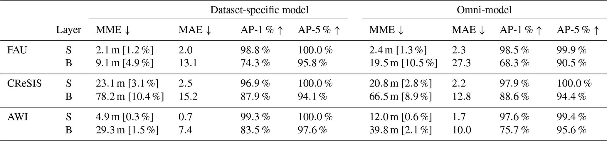
Overall, the results are promising, with high AP-1 % and AP-5 % values and low MME and MAE values for most combinations. Still, dataset- and model-specific discrepancies exist.

5.3.1 Ice surface predictions

The predictions for the ice surfaces are nearly perfect for all subsets and all models. The three subset models even achieve 100 % accuracy for the AP-5 %. Hence, the remaining discrepancies are likely significantly influenced by measurement inaccuracies, noise, and general model variance. Therefore, we will only consider the task of ice bottom delineation to assess model performance.

5.3.2 Ice bottom predictions

For the ice bottom predictions, the differences in the MME between the three subsets are more pronounced than for the MAE, which can be attributed to the different VRs. The MAE difference between the FAU and CReSIS subsets is small, while the MAE on the AWI subset is substantially lower than both. The AP-1 % is lower for the FAU subset than for the AWI and CReSIS subsets. Interestingly, this difference between subsets is relativized for AP-5 %. This means that most incorrect predictions for FAU are in the 1 % to 5 % error range. The same is true for the AWI subset. For the CReSIS data, this effect is not as strong. Here, the AP only increases from 87.9 % for the 1 % error rate to 94.1 % for the 5 % error rate.

5.3.3 Omni-model

The omni-model shows persistently higher MME and MAE values and lower AP-1 % and AP-5 % values for the FAU and AWI subsets than the dataset-specific models. In detail, it only achieves an MME of 19.5 m and 39.8 m and an AP-1 % of 68.3 % and 75.7 %, respectively. We attribute the lower performance of the omni-model to the substantial domain shift between the three subsets and the fact that the FAU and AWI subsets are significantly smaller than the CReSIS subset. For the CReSIS subset, the omni-model outperforms the dataset-specific model. In particular, it achieves an MME of 66.5 m and an AP-1 % of 88.6 %. These results suggest that there can be a benefit from more training data even with the domain shift. However, the domain shift makes the generalization to underrepresented or new domains difficult.

5.3.4 Influence of study sites

Table 3 divides the results of the subset-specific models by study site and thermal regime.

Table 3 Overview of the influence of geographical and glaciological factors on the performance in detecting the ice bottom. We differentiate between the subset, the study site, and the general thermal regime. For the performance analysis, we compare the MME, MAE, AP-1 %, and AP-5 % as defined in Sect. 5.1. To contextualize the MME, we annotate the relative error to the mean measured ice thickness of the specified test set study site behind the MME. Note that for the AWI subset-specific model, we utilized the weights of the omni-model as a starting point to stabilize training. We conducted the evaluation on the test set and averaged the results over five runs to minimize statistical errors. The analyzed models were the subset-specific models.

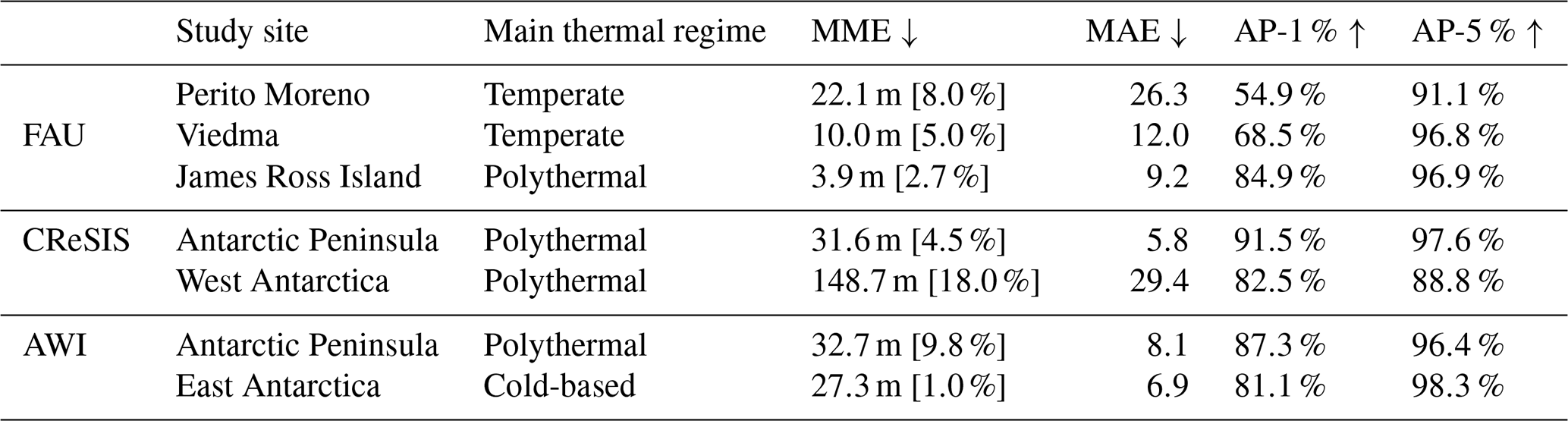
For the FAU subset, the Perito Moreno and Viedma predictions are quantitatively worse than the ones from JRI. A key difference between Perito Moreno, Viedma, and JRI is the thermal regime. The first two are temperate glaciers, while JRI contains polythermal ice. Besides the higher water content in Perito Moreno and Viedma, both are also substantially deeper than JRI in most areas. They even have areas with ice thicker than the 700 m maximum penetration depth of the employed radar system. Viedma and JRI also feature moraine material several meters thick on the glacier surface. These rock and debris deposits are not penetrable by the wavelets and thus create radar shadows below them or substantially decrease the amount of reflected energy.

If we look at the associated radargrams, we can mostly see a relatively stable and clear prediction for JRI. On the other hand, Viedma and Perito Moreno have much stronger differences from the ground truth. Especially in deep and noisy regions, the models struggle. Figure 5 shows example traces for the three study sites of the FAU subset.

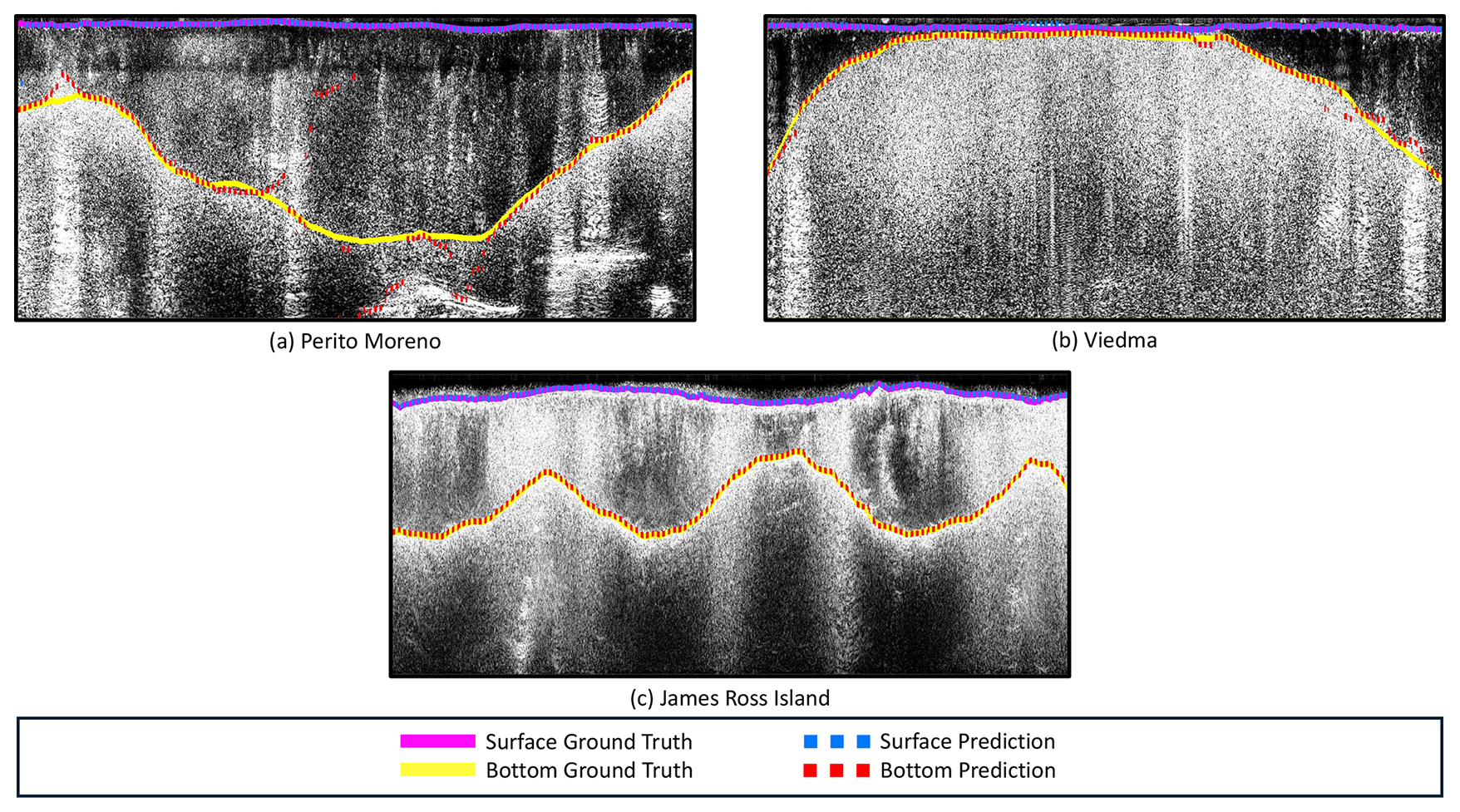
Figure 5 Visualization of the subset-specific model's performance on the FAU subset. Panel (a) shows trace 3000–5500 of the third flight over Perito Moreno, panel (b) depicts traces 5000–7500 of the second flight over Viedma, and panel (c) presents traces 5000–7500 from the first section of the 2017 flights over James Ross Island.

Between the Antarctic Peninsula and West Antarctica study sites of the CReSIS subset, there are strong differences in the quantitative analysis. The MME and MAE values exhibit a difference of approximately a factor of 5, while the AP-1 % and AP-5 % are approximately 9 % apart. In the qualitative analysis, we can see that the predictions in both regions actually follow the ground truth closely. However, sometimes the predicted ice bottom layer makes a jump and the actual ice surface is predicted to be the ice bottom. We call this “ice boundary collapse”. Examples of this phenomenon can be seen in Fig. 6.

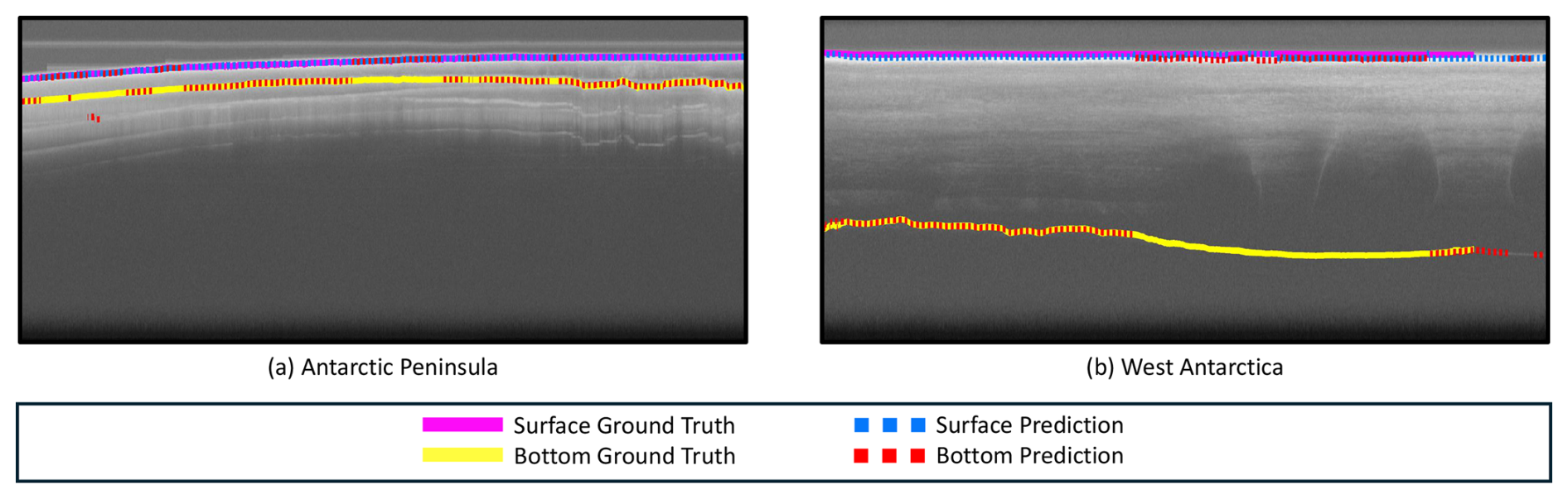
Figure 6 Visualization of the subset-specific model's performance on the CReSIS subset. Panel (a) presents traces 2000–4500 from mission PEN4 in the Antarctic Peninsula (PEN4_01_001). Panel (b) presents traces 2000–4500 from mission TSK2 in West Antarctica (TSK2_07_003).

For the AWI subset, the results for East Antarctica are generally more favorable than those for the Antarctic Peninsula. This result is consistent with the observation on the FAU subset that the algorithm performs better for colder ice than for warmer ice. The only exception is the AP-1 %, where the Antarctic Peninsula slightly outperformed East Antarctica. This result suggests that a large majority of the wrong predictions in East Antarctica are between the 1 % and 5 % interval and that our algorithm struggles to pinpoint the exact location of the ice bottom. We can confirm this behavior in the qualitative analysis, where the prediction is sometimes slightly above or below the ground-truth line but follows it closely overall. Similarly, the predictions for the Antarctic Peninsula also appear to be very accurate but contain more occasional outliers. Figure 7 depicts the predictions for both East Antarctica and the Antarctic Peninsula.

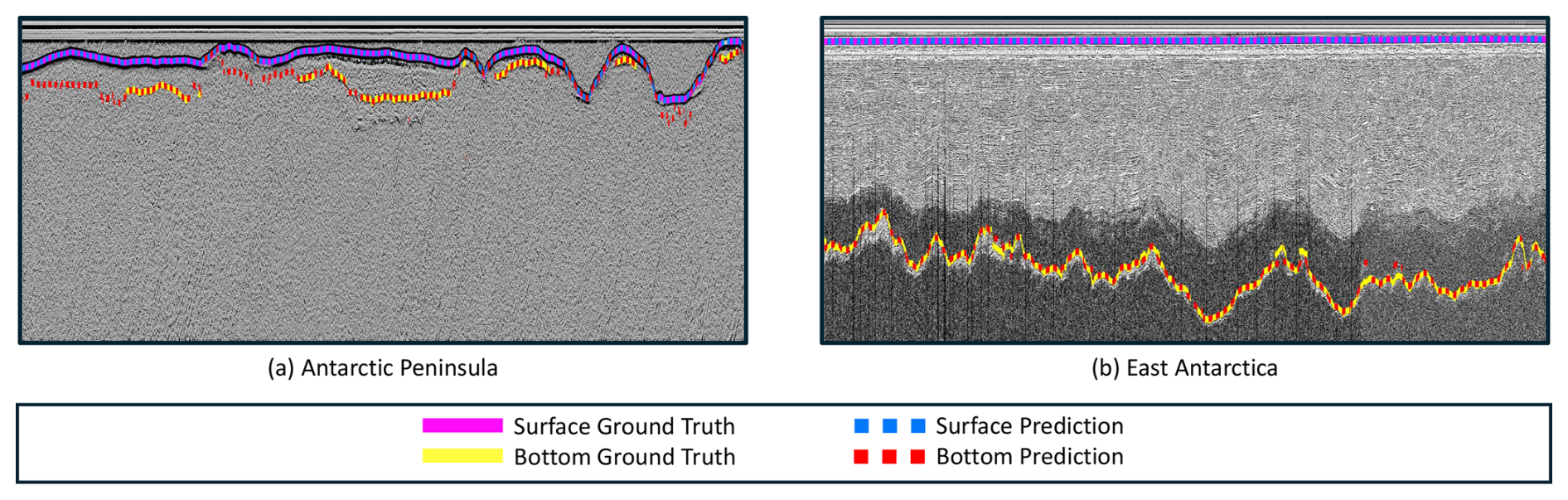
Figure 7 Visualization of the subset-specific model's performance on the AWI subset. Panel (a) depicts traces 21 000–23 500 from the 2014 flight in the Antarctic Peninsula. Panel (b) presents traces 7837–9787 from the 1999 flight in East Antarctica.

5.3.5 Loss function

To assess the performance of our combined loss function, we conducted a small ablation study. Specifically, we evaluated two additional experiments in which we replaced the combined loss with each of its individual components: in the first setup, we trained the model with the cross-entropy loss, and in the second setup, we trained it only with the distance loss. We compare the results of these two configurations with the combined loss in Table 4.

Table 4 Summary of our ablation study regarding the proposed modifications to the loss function. For every variation of the loss function, we trained a subset-specific model and compared the performance based on the MME and AP-1 % of the ice bottom layer. We conducted the evaluation on the test set and averaged the results over five runs to minimize statistical errors. To contextualize the MME, we annotate the relative error to the mean measured ice thickness of the specified test set study site behind the MME. Note that for the AWI subset-specific model, we utilized the weights of the omni-model as a starting point to stabilize training, which was also trained with the specified loss function.

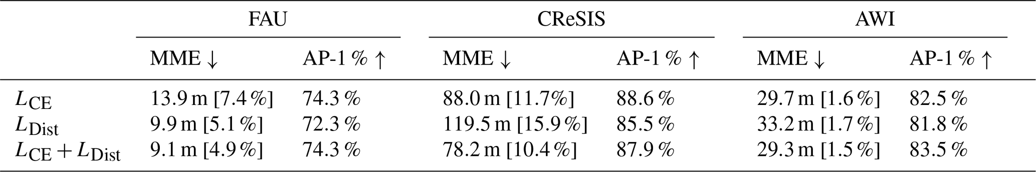
For the FAU subset model, the distance loss improves the MME but not the AP-1 %. In contrast, the cross-entropy is better for the AP-1 % but not for the MME. The combination of both losses results in an improved MME, while AP-1 % remains the same. The results for the CReSIS subset are less clear. It is evident that the distance loss alone does not enhance the MME or AP-1 %. However, the combined loss demonstrates the most optimal outcome in relation to the MME, while the AP-1 % is only slightly worse in comparison to CE alone. Similar to the CReSIS results, the distance loss alone does not improve the MME compared to the cross-entropy for the AWI subset. However, the combined loss provides the best results with a higher AP-1 % value.

5.4 Discussion and outlook

One apparent influence on the quality of the ice bottom prediction is the primary thermal regime of the region. In general, the warmer the ice, the less reliable the prediction. The reason behind this is probably the influence of water on the signal, as well as the higher likelihood of a heavily crevassed surface. Temperate ice generally contains water, as most of the ice is close to or at the pressure melting point. Water absorbs the recorded signal, leading to higher noise with increased depth and strong attenuation. Hence, the model's performance naturally decreases as the associated radargrams are more challenging to interpret. Polythermal glaciers, contrary to temperate glaciers, do not exhibit ice at the pressure melting point everywhere. Instead, elevated temperatures are usually confined to zones of fast flow driven by frictional heating or to marginal areas of the glacier. Hence, the effects are not as detrimental as for entirely temperate glaciers.

Another interesting observation is the difference between temperate and polythermal ice regarding the AP-1 % and AP-5 %. The AP-1 % of temperate ice is significantly lower than for polythermal ice. However, the AP-5 % is relatively similar for both types of ice. While it is natural for the difference to decrease at higher error intervals, the change in this case is still very drastic. To put this into perspective, Viedma and James Ross Island were 16.4 percentage points apart on the AP-1 % but on the AP-5 % only 0.1 percentage points. A possible explanation for this could lie in the meltwater at the base of the ice. Temperate ice more commonly collects meltwater at its base than polythermal ice. Since water absorbs the signal, the exact position (AP-1 %) becomes difficult to identify. However, the general position (AP-5 %) is still clear because the water is only at the base. Besides the thermal regime and average depth, the presence of debris usually plays a significant role in radio-echo sounding. Interestingly, the quantitative results of JRI and Viedma indicate that the presence of debris did not play a major role in the model's performance compared to depth and thermal regime. However, we suspect that the numbers do not capture the effect of debris very well since the debris likely absorbed the signal entirely. Thus, the expert could not create ground-truth labels for these parts, which makes the effect of debris on the model's performance not accurately measurable with numerical methods.

One of the more prominent and recurring phenomena in the CReSIS model's predictions is the collapse of ice boundaries. In ambiguous cases, the model shows a bias toward predicting the ice bottom close to the ice surface or as the ice surface. One explanation could be that the CReSIS data are differentiated and thus represent only the change in amplitude. That makes it challenging to distinguish whether the peak of the ice surface and ice bottom overlap or the ice bottom is not visible. The problem gets further amplified by noise and artifacts, such as multiples. They can exhibit similar patterns as the ice bottom, making the model biased toward predicting the ice bottom as the ice surface when in doubt.

Furthermore, we believe that the influence of the ice boundary collapse is also reflected by the quantitative analysis of the different CReSIS study sites. As West Antarctica generally contains thicker ice sheets than the Antarctic Peninsula, the average distance between the ice boundaries significantly increases. Thus, a wrong prediction of the ice bottom as ice surface leads to a considerably higher MAE and MME for West Antarctica than the Antarctic Peninsula. However, the ice boundary collapse is likely not the only reason for this effect as the AP-1 % and AP-5 % are also lower for West Antarctica than the Antarctic Peninsula. Hence, thicker ice sheets might be naturally more challenging.

Nonetheless, future research should address ice boundary collapses as they tremendously affect performance. Larger contexts, additional post-processing steps, or recurrent neural networks could help stabilize the predictions as they incorporate more information. Another interesting problem to explore is the performance drop from subset-specific models to the omni-model. Our results indicate that the domain shift between the subsets is too prominent for a simple omni-model to catch up on all subset characteristic features. Hence, models cannot utilize the full benefits of a larger dataset when they are recorded and processed differently. In particular, domain shift techniques could help with this challenge, but also more advanced regularization techniques, e.g., spatial dropout, could prevent the model from focusing too much on a single domain (Tompson et al., 2015). In Appendix D, we show that a uniform sampling strategy can also help mitigate the domain shift.

We believe that our framework is a step towards a potential fully automated generation of ice thickness maps based on RES data and that our work represents an advancement toward validating survey data in the field.

6 Conclusions

This paper presents the first benchmark framework for delineating the ice boundary in RES data. The included dataset “IceAnatomy” contains hundreds of kilometers of processed, labeled, and georeferenced RES data from three different sources (FAU, CReSIS, AWI). Since all sources employ a different radar system and processing methods, “IceAnatomy” offers a wide range of varying amplitude spectrums, vertical resolution of the two-way travel time, and width resolutions, making it applicable to a multitude of settings. Furthermore, it also features different geographical factors, such as study sites and thermal regimes, allowing for in-depth analysis of the models and their behavior in different geographical scenarios.

To fairly compare different models in the future, we provide an official train and test split for each source of the dataset. This enables the development of not only an omni-model trained on the entire dataset but also specialized subset-specific models trained on one of the three sources. We trained and evaluated a baseline model for each of these scenarios. In our experiments, the subset-specific models provide the most promising results with MMEs of 2.1 m [1.2 %], 23.1 m [3.1 %], and 4.9 m [0.3 %] for the ice surface and 9.1 m [4.9 %], 78.2 m [10.4 %], and 29.3 m [1.5 %] for the ice bottom depending on the source.

Previous work has already demonstrated the effectiveness of automatic approaches for ice boundary extraction but lacked a common method for accurately comparing models. With this benchmark framework, we hope to address this issue by unifying and standardizing both training and evaluation schemes. We hope that this benchmark dataset will encourage more scientists to engage in this challenging and important research area. Deep learning models that extract the ice boundary can greatly speed up the processing of RES data. As a result, the ice thickness and, consequently, the subglacial topography can be determined more quickly after a field survey.

Appendix A: Additional hyperparameters

This section gives an overview of the hyperparameters in our employed U-Net from Sect. 4.2. The input dimension of our U-net is ($\mathrm{1024},\mathrm{512},\mathrm{1}$) ($H,W,\mathrm{1}$), which then gets scaled according to the depth level of the encoder or decoder. Inside the network, we down- and up-sample our feature map five times each while scaling the feature dimension according to the depth-level-dependent value of $[\mathrm{8},\mathrm{16},\mathrm{32},\mathrm{64},\mathrm{64},\mathrm{128}]$. To reduce the risk of overfitting, we also utilize dropout layers inside the ResBlocks with a probability of 10 %. For the loss function, we employed our proposed combined loss function. Since the numerical value of the distance loss is significantly higher than that of the classification loss, we had to weigh the individual components. In detail, we chose the weights w_{s_class}=0.5, w_{b_class}=1.0, w_{s_dist}=0.05, and w_{b_dist}=0.1 as they performed the best in preliminary experiments.

Appendix B: ResBlock design

To provide a better understanding of the network architecture, this section examines one of its core components: the ResBlock from Esser et al. (2020). Its structure, shown in Fig. B1, comprises several components. First, it starts with a group normalization layer (Wu and He, 2018) that normalizes the data in groups of channels to increase stability during training. Next, a swish activation (Ramachandran et al., 2017) function adds nonlinearity to the ResBlock so the network can learn more complex patterns. The activation is followed by a two-dimensional convolution layer that processes and combines the visual features by applying convolutional operations. This is followed by another group normalization and swish activation function before a regular dropout layer (Hinton et al., 2012) is applied. The dropout layer randomly withholds information during training to improve generalization and prevent the model from overfitting – a process in which the model develops a strong bias towards the training data. After the dropout layer, another two-dimensional convolutional layer is applied. Finally, a residual connection (He et al., 2016), a shortcut from the start of the ResBlock to the end through a convolution layer, is added to the output of this sequence of layers to improve the gradient flow in the network.

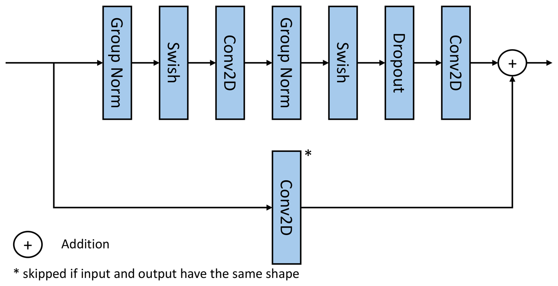
Figure B1 Structure of the residual block employed in our deep learning model. The arrangement is based on the design of Esser et al. (2020).

Appendix C: Loss function details

The formulas of the classification and distance-based loss are as follows.

$$\begin{array}{}\text{(C1)}& {\displaystyle }\begin{array}{rl}{L}_{\text{CE}}& =-\sum _{c\in C}{x}_c(\mathrm{1}-{\mathit{ϵ}}_c)\log \left(p\right(x_c\left)\right)\\ & +{\displaystyle \frac{{\mathit{ϵ}}_c(\mathrm{1}-x_c)\log \left(p\right(x_c\left)\right)}{\left|C\right|}}\end{array}\text{(C2)}& {\displaystyle }\begin{array}{rl}{L}_{\text{class}}& ={\displaystyle \frac{w_{\text{s\_class}}}{\left|{\widehat{Y}}_{\text{s}}\right|}}\sum _{{\widehat{y}}_{\text{s}}\in {\widehat{Y}}_{\text{s}}}{L}_{\text{CE}}\left({\widehat{y}}_{\text{s}}\right)\\ & +{\displaystyle \frac{w_{\text{b\_class}}}{\left|{\widehat{Y}}_{\text{b}}\right|}}\sum _{{\widehat{y}}_{\text{b}}\in {\widehat{Y}}_{\text{b}}}{L}_{\text{CE}}\left({\widehat{y}}_{\text{b}}\right)\end{array}\text{(C3)}& {\displaystyle }\begin{array}{rl}{L}_{\text{dist}}& ={\displaystyle \frac{w_{\text{s\_dist}}}{\left|{\widehat{Y}}_{\text{s}}\right|}}\sum _{{\widehat{y}}_{\text{s}}\in {\widehat{Y}}_{\text{s}}}\langle d\left(y_{\text{s}}\right),\mathit{\sigma }\left({\widehat{y}}_{\text{s}}\right)\rangle \\ & +{\displaystyle \frac{w_{\text{b\_dist}}}{\left|{\widehat{Y}}_{\text{b}}\right|}}\sum _{{\widehat{y}}_{\text{b}}\in {\widehat{Y}}_{\text{b}}}\langle d\left(y_{\text{b}}\right),\mathit{\sigma }\left({\widehat{y}}_{\text{b}}\right)\rangle \end{array}\end{array}$$

w_{s_class}, w_{b_class}, w_{s_dist}, and w_{b_dist} are the respective weights for a weighted combination of the single loss parts, ϵ_c is the smoothing factor, C specifies the column, 〈〉 is the dot product, σ is the softmax function that converts the model's outputs into probabilities, $|.|$ is the cardinality of a set, and d is the function that creates a vector filled with the column-wise distance map given the respective column of the label.

Appendix D: Additional experiments

Since the three subsets of IceAnatomy differ in size, we also investigate whether a uniform sampling strategy, where samples are drawn equally from each subset, could help the omni-model achieve the performance of the domain-specific models on the AWI and FAU subsets. From our results in Table D1, we can see that a uniform sampling strategy does lead to improvement for the AWI and FAU subsets. In the case of the AWI subset, the omni-model even outperforms the domain-specific model. However, in the case of the FAU subset, we are still below the domain-specific model. We reason that the domains of the AWI and CReSIS subsets are significantly closer than the FAU subset as these two subsets contain differentiated radargrams. We, therefore, believe that domain shift remains an important area for future research.

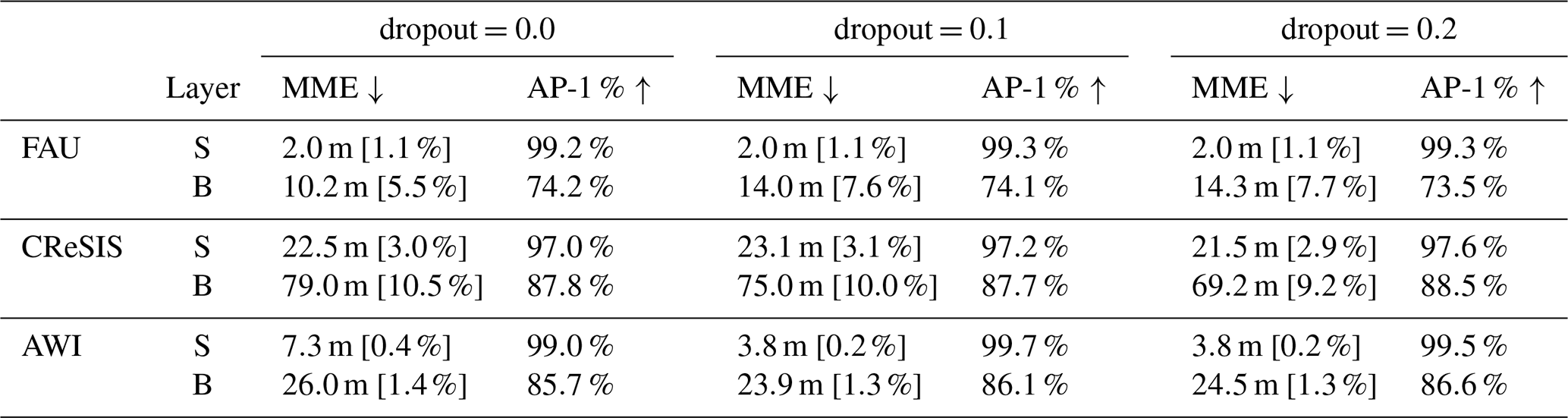
In addition to the uniform sampling, we also investigated how different hyperparameter setups regarding learning rate and regularization would affect the benchmark model. From the results in Tables D2 and D3, we can see that different hyperparameter setups favor different subsets of IceAnatomy. However, there seems to be no universal optimal setup.

Table D1 Overview of the performance of our omni-model with uniform sampling. We distinguish the layer prediction into two classes: the ice surface (S) and the ice bottom (B). We compare the model's performance on the MME, MAE, AP-1 %, and AP-5 % as defined in Sect. 5.1. To contextualize the MME, we annotate the relative error to the mean measured ice thickness of the specified test set study site behind the MME. We conducted the evaluation on the test set and averaged the results over five runs to minimize statistical errors.

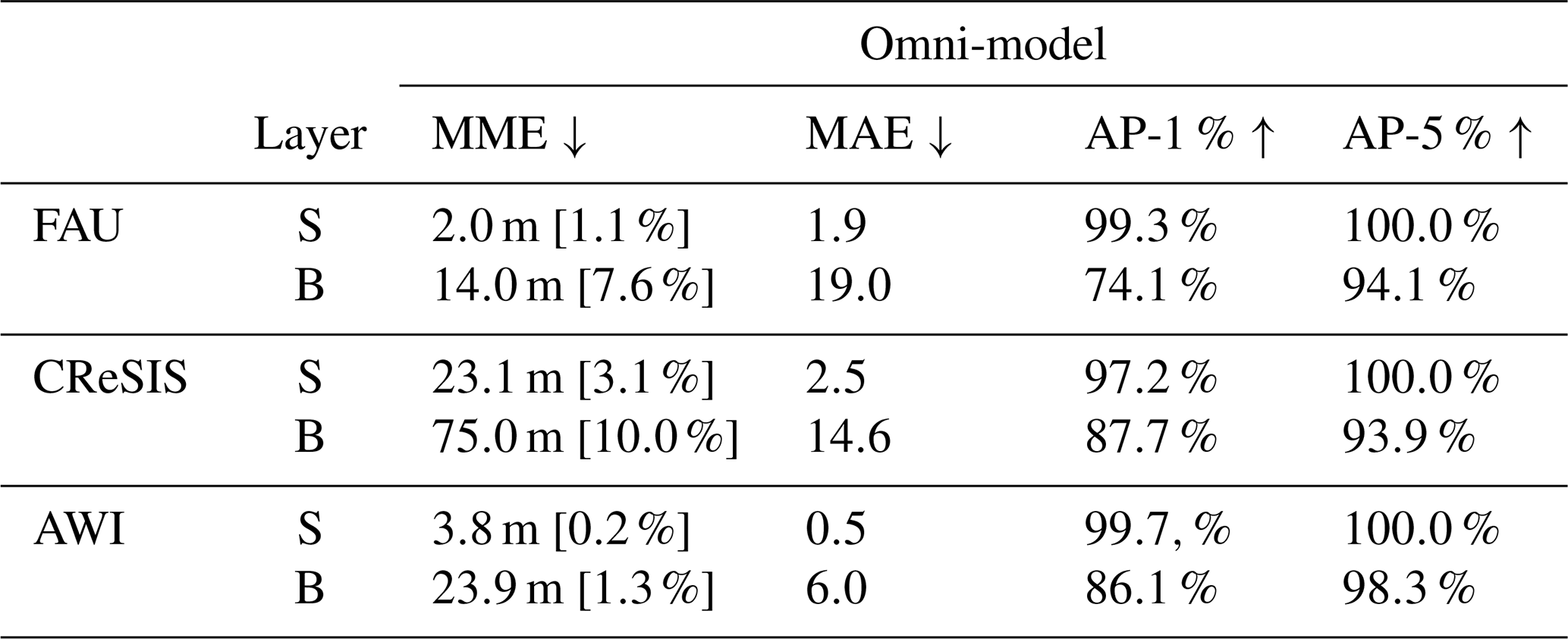
Table D2 Overview of the performance of our omni-model with different learning rates and uniform sampling. We distinguish the layer prediction into two classes: the ice surface (S) and the ice bottom (B). We compare the model's performance on the MME and AP-1 % as defined in Sect. 5.1. To contextualize the MME, we annotate the relative error to the mean measured ice thickness of the specified test set study site behind the MME. We conducted the evaluation on the test set and averaged the results over three runs to minimize statistical errors. Note that for lr =0.005 we averaged over five runs, as we had those values from previous experiments.

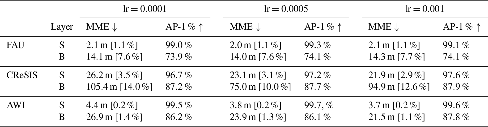
Table D3 Overview of the performance of our omni-model with different learning rates and uniform sampling. We distinguish the layer prediction into two classes: the ice surface (S) and the ice bottom (B). We compare the model's performance on the MME and AP-1 % as defined in Sect. 5.1. To contextualize the MME, we annotate the relative error to the mean measured ice thickness of the specified test set study site behind the MME. We conducted the evaluation on the test set and averaged the results over three runs to minimize statistical errors. Note that for dropout =0.1 we averaged over five runs, as we had those values from previous experiments.

Appendix E: Translations of the vertical resolutions

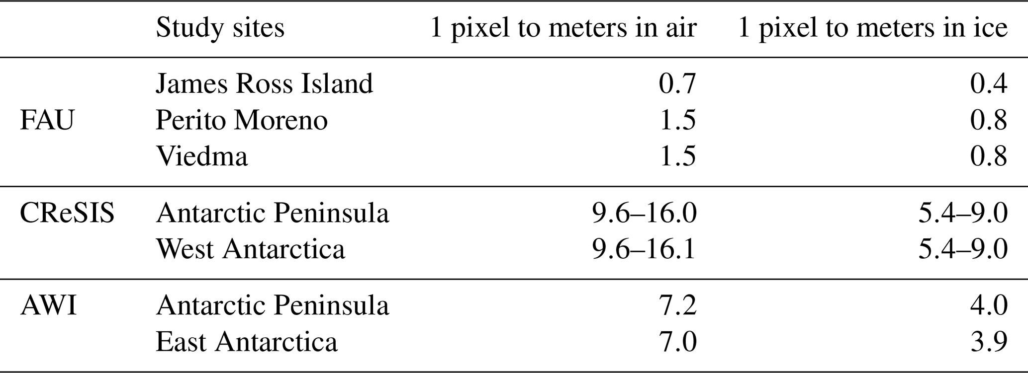
While the vertical resolution of the two-way travel time approximates the granularity of the specific radargrams, it is challenging to interpret for a real-world scenario. To simplify interpretation, we provide a simple conversion in Table E1 given a fixed radargram height of 1024 pixels. Although the vertical resolution was fixed for each data source, the ratio of pixels to meters varies depending on the flight, the original height of the radargram, and the chosen radargram height, as well as between the air and ice layers. Interestingly, this table also offers an estimate of the lower error bound introduced by discretizing the continuous height values into pixels. Since the introduced model does not interpolate between pixels, decimal pixel heights cannot be represented accurately. The problem gets further amplified by downscaling the images to a lower resolution, as the pixel-to-meter ratio rises proportionally.

Table E1 A conversion table that translates pixels to meters given a fixed height of 1024 pixels.