the Creative Commons Attribution 4.0 License.
the Creative Commons Attribution 4.0 License.
 | 24 Oct 2025
Comprehensive assessment of stress calculations for crevasse depths and testing with crevasse penetration as damage
Sophie Nowicki
Kristin Poinar
Crevasse depth calculations with the zero stress approximation or linear elastic fracture mechanics are used in many applications, including calving laws, determination of stable cliff heights, shelf vulnerability to collapse via hydrofracture, and damage evolution in ice. The importance of improving the representation of these processes for reducing sea level rise uncertainty makes careful calculation of stresses for crevasse depths critical. The resistive stress calculations used as input for these crevasse predictions have varied across studies, including differences such as the use of flow direction stress versus maximum principal stress, the inclusion of crevasse-parallel deviatoric stress, and calculation of effective strain rate. We provide a systematic review of how resistive stress calculations found in the literature result in differing crevasse depth predictions and where these differences are most pronounced. First, we study differences in crevasse depths calculated from idealized representative strain rate states and then from velocity observations of several Antarctic ice shelves. To test whether the patterns of crevasse depths predicted from these stresses have a strong connection to bulk rheology, we use crevasse penetration as damage and compare predicted velocities from an ice sheet model against observed velocity. We find that the selection of stress calculation frequently changes crevasse depth predictions by a factor of 2 or more and that differences are pronounced in shear margins and regions of unconfined, spreading flow. The most physically consistent calculation uses the maximum principal stress direction, includes the vertical strain rate from continuity in the effective strain rate calculation, and uses three-dimensional resistive stress (). However, this calculation has rarely been used to date in studies requiring crevasse depth predictions. We find that this most physically consistent stress calculation produces a damage pattern that qualitatively matches surface features and quantitatively reproduces observed velocities better than other stress calculations; we therefore recommend the use of this stress calculation. This result also suggests that other stress calculations likely overpredict shear margin vulnerability to hydrofracture and would overpredict calving in shear margins and spreading fronts when implemented in the crevasse depth calving law.
- Article
(14971 KB) - Full-text XML
-
Supplement
(2786 KB) - BibTeX
- EndNote


Ice damage evolution, ice shelf collapse, and calving are three related processes that lead to increased ice flow rates into the ocean, increasing sea level rise rates. High uncertainty in modeling these processes propagates into uncertainty in the future sea level rise contributions of the Greenland and Antarctic ice sheets (van de Wal et al., 2022). Ice shelves restrain upstream ice flow via buttressing, which is back stress from shear load transmitted to embayment walls or compressive loading caused by pinning points (Fürst et al., 2016; Gudmundsson, 2013; Schoof, 2007). Damage evolution can reduce the amount of buttressing provided by the shelf to the upstream ice. This causes an increase in speed of the upstream ice and thus a higher rate of sea level contribution (e.g., Khazendar et al., 2015; Lhermitte et al., 2020). This damage evolution, sometimes aided by high surface meltwater availability, can also lead to collapse of entire ice shelves. Shelf collapse fully removes buttressing, so the corresponding change in speed of upstream ice can be large, as seen for the inlet glaciers into the former Larsen B shelf (e.g., Rignot et al., 2004; Rott et al., 2011). While retreat from increased calving is less dramatic than a sudden ice shelf collapse, both can result in increased in glacier velocities because of termini in locations that provide less back stress. This effect was demonstrated via ice sheet modeling of Sermeq Kujalleq (Jakobshavn Isbrae) that found terminus position change caused the majority of the doubling of the glacier's velocity (Bondzio et al., 2017). Finally, in the case of ice shelf collapse, initialization of retreat through the rapid, brittle mechanism of marine ice cliff instability (MICI) has been proposed if cliffs are exposed that ice strength cannot support (Bassis and Walker, 2011; Pollard et al., 2015).
A commonality between these processes is the importance of the presence and size of crevasses. For damage evolution, Sun et al. (2017) used crevasse penetration directly as damage. Albrecht and Levermann (2014) and Borstad et al. (2016) proposed damage laws that do not directly consider crevasse depth but use threshold stresses for damage initiation that can be linked to crevasse initiation by linear elastic fracture mechanics (LEFM). For ice shelf vulnerability to hydrofracture, Lai et al. (2020) demonstrated that crevasse presence predictions with LEFM align with locations where crevasses are observed. They then identify regions that both provide buttressing and are expected to be crevassed to assess where hydrofracture could cause shelf collapse that will yield increased upstream velocity. Calving has been modeled directly based on the predicted crevasse depths from local stresses in the crevasse depth calving law (Benn et al., 2007; Nick et al., 2010), which has been used by many subsequent studies (Amaral et al., 2020; Benn et al., 2023; Choi et al., 2018; Todd et al., 2018). Berg and Bassis (2022) also showed the importance of crevasse advection from upstream for modeling calving. Finally, the limit on cliff height for stability under the MICI theory used crevasse penetration with the zero stress approximation (Bassis and Walker, 2011). With this need for crevasse depths in modeling these processes, researchers have proposed several physical theories for making crevasse depth predictions.
The three primary theories for crevasse depth predictions vary in their assumptions about ice's strength and the effect of a crevasse on the surrounding stress field. First, the zero stress approximation (Nye, 1955) assumes ice has no tensile strength and that the presence of a crevasse does not modify the surrounding stress field. Second, the horizontal force balance method (Buck, 2023) maintains the assumption that ice has no tensile strength but considers the impact of reduced ice thickness from surface and basal crevasses, air or water pressure in surface crevasses, and water pressure in basal crevasses on force balance. Finally, linear elastic fracture mechanics (LEFM), applied to crevasses by Weertman (1973) and many subsequent researchers, considers the stress-amplifying effect of crevasse geometry and allows laboratory measurements of a material's resistance to fracture to be used for predicting fracture in more complex stress states. LEFM tends to increase predicted crevasse depths relative to the zero stress approximation for isolated crevasses and allows for the determination of threshold stress for crevasse formation based on ice's fracture toughness and the size of the initial flaw (a small defect in the ice surface) (e.g., Lai et al., 2020; van der Veen, 1999). Studies have assessed the differences in crevasse depth predictions between these calculations and compared them to observations (Mottram and Benn, 2009; Enderlin and Bartholomaus, 2020). A key input to these calculations is the full stress as a function of ice depth, although not all studies have used the full stress.
The crux of the problem is what component or components of ice stress control the propagation of a crevasse. The calculation steps to go from observed strain rate and temperature to the full stress have varied significantly across crevasse depth studies. For example, five different stress calculations can be found in six studies that use crevasse depths for damage evolution, shelf collapse vulnerability, calving, and comparison to observed crevasses (Amaral et al., 2020; Choi et al., 2018; Enderlin and Bartholomaus, 2020; Lai et al., 2020; Mottram and Benn, 2009; Sun et al., 2017). The differences in stress calculations come from the stress orientation (flow direction or maximum principal), use and calculation of effective strain rate, and inclusion of the deviatoric stress running parallel to the crevasse in the resistive stress calculation. Two studies (Choi et al., 2018; Lai et al., 2020) have tested their methods across two different stress calculations, but to date no study has comprehensively surveyed the range of stress calculations used for crevasse depths.
We seek to determine more broadly whether and where selection of stress calculation is significant in determining crevasse depths. In the background, we will present the differences in stress calculations across studies in more detail. Then, in the Methods section, we show crevasse sizes for simple idealized strain rate states with each calculation before plotting crevasse penetration on real ice shelves. We compare predicted crevasse penetration against observed surface features and velocity to assess whether the results with each stress calculation are realistic. With stress calculation versions that seem plausible, we then study the connection between calculated crevasse depths and bulk ice rheology. We do this by testing the ability of crevasse penetration as damage to yield observed velocity fields with an ice sheet model. We find that common assumptions made when calculating resistive stress from strain rates frequently lead to differing crevasse depths by a factor of 2 or more and that the most physically based calculation creates crevasse penetration that best reproduces observed velocities when used as damage in an ice sheet model (Borstad et al., 2012; Larour et al., 2012).
2.1 Stress contributions for crevasse calculations
The viscous flow of ice is driven by deviatoric stress, the component of the Cauchy stress that does not cause volume change during deformation. Brittle failure is driven by the Cauchy stress itself. If ice is pulled on in equi-triaxial tension, it will not flow but it may fracture. For this reason, the lithostatic pressure that increases with depth does not affect viscous deformation but does suppress crevasse extension. (Change in lithostatic pressure with distance causes flow, but pressure itself does not.) The Cauchy or full stress as a function of depth in the ice column used to determine crevasse sizes comes from the combination of resistive stress, lithostatic pressure, and water pressure (Fig. 1).
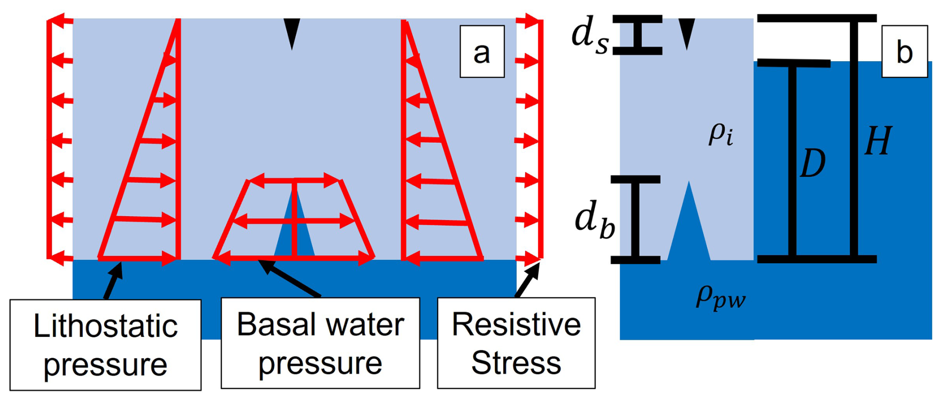
Figure 1Diagrams of (a) stress and pressures that control crevasse sizes and (b) variables used in crevasse size calculations. Physical property values and variable descriptions are provided in Tables A1 and A2 in Appendix A.
The resistive stress is the stress pulling a crevasse open because of local ice extension. In remote-sensing- or field-measurement-based workflows, deviatoric stresses are calculated from strain rates using Glen's flow law, from which resistive stress may then be calculated. Within Glen's flow law, the selection of depth-averaged temperature, depth-averaged rigidity, a vertical temperature profile, or surface and basal temperatures will have large impacts (Coffey et al., 2024) but is not considered here. Change in ice rigidity with firn density is also important in specific settings (Clayton et al., 2024; Gao et al., 2023) but also not considered here. The differences in stress calculations we consider are in the stress direction selected, the calculation of effective strain rate, and the consideration of deviatoric stress in the crevasse-parallel direction when calculating resistive stress.
Lithostatic pressure comes from the weight of ice above the vertical position in the ice column and counters the resistive stress to prevent crevasse extension. For surface crevasses, firn properties are again critical, with density changing the increase in lithostatic pressure with depth (Clayton et al., 2024; Gao et al., 2023; van der Veen, 1998a). In the case of meltwater in a surface crevasse, water pressure acts against the lithostatic pressure, allowing for more crevasse extension. Water in crevasses has been included as fixed depth (e.g., Benn et al., 2007) or as maintaining a water table height (e.g., van der Veen, 1998a). The water table height approach leads to hydrofracture once a crevasse reaches the water table (or potentially a little beyond for LEFM) due to water's density exceeding that of ice. Firn porosity can reduce the pressure loading transmitted into the ice itself (Meng et al., 2024). Water in basal crevasses again acts against lithostatic pressure. In floating ice in hydrostatic equilibrium, the lithostatic pressure and water pressure at the bottom surface of the shelf are equal. With vertical position, water pressure decreases more than lithostatic pressure according to their densities. This adds net compression with rising crevasse height, but at a much slower rate than lithostatic pressure alone for surface crevasses, resulting in the prediction of much taller basal crevasses. This remains so even when the relative softness of basal ice near melting temperature is considered in the calculation, as shown later in the Results section (Table 3).
2.2 Zero stress approximation
The zero stress approximation (Nye, 1955) assumes that ice has no tensile strength such that a crevasse extends as far into ice as tension is present. When the resistive stress is tensile, then, surface crevasses will extend down until the lithostatic pressure of ice equals the resistive stress. Weertman (1980) and Jezek (1984) used this criterion to calculate basal crevasse heights on ice shelves by including the pressure from ocean water. The crevasse depth calving law (Benn et al., 2007; Nick et al., 2010) applies the zero stress approximation for prediction of calving by limiting the terminus position to where surface crevasses do not reach the waterline and the combined surface and basal crevasse sizes do not penetrate the full thickness of ice. The water level in surface crevasses can thus be used as a tuning variable (e.g., Choi et al., 2018; Amaral et al., 2020). Subsequent studies based on the zero stress approximation (Bassis and Walker, 2011; Sun et al., 2017) have applied the equations in Nick et al. (2010) for surface and basal crevasses, which we reprint here for easy reference. Surface crevasse depth, ds, is given by
where Rxx is the resistive stress perpendicular to the crevasse, ρi is ice density, ρmw is meltwater density, dmw is the depth of meltwater in the crevasse, and g is gravitational acceleration (Fig. 1). Basal crevasse height, db, is given by
where ρpw is the density of the proglacial water (lake or ocean) and Hab is the height above buoyancy, defined as
where H is ice thickness and D is the depth of ocean or lake water in contact with the ice cliff. Height above buoyancy is zero for ice shelves assumed to be in hydrostatic equilibrium. The resistive stress, Rxx, in Nick et al. (2010) is the one-dimensional form and is given as
where is the crevasse-perpendicular strain rate, A is the rate parameter in Glen's flow law, and n is the flow law exponent. This is the crevasse-perpendicular deviatoric stress multiplied by a factor of 2. More generally, the resistive stress is defined as the full stress minus the lithostatic pressure (van der Veen, 2013). Assessing three-dimensional implementations of Eq. (4) that consider effective strain rate (ice softening from multiple directions of deformation) and crevasse-parallel stress is the primary focus of our work. We will work with the zero stress approximation because it is simple and will represent the same general pattern of change in crevasse depth predictions with stress calculation as would result in the other methods for predicting crevasse depths presented next.
2.3 Horizontal force balance
The horizontal force balance method (Buck, 2023) maintains the zero stress criterion for ice failure but includes the self-amplifying effect of crevasses themselves on the force balance of the region of ice. As surface crevasse depth and basal crevasse height increase, force is carried by a smaller cross section of ice (here termed the ligament), and basal water pressure, as well as air or meltwater pressure in surface crevasses, adds force that must be counteracted by additional force from ice deformation. These effects mean that, with increasing resistive stress and thus crevasse sizes, there will be an increasing additional crevasse size relative to those predicted by the zero stress approximation. The ratio of the increased stress in the remaining ligament (Rxx,1) relative to the original resistive stress (Rxx,0) for isothermal ice is
where Kb is the buttressing number, which normalizes the depth-averaged stress relative to a floating ice cliff and can be calculated as in Fürst et al. (2016), and dw and dpw are the distances between the ice surface and zero water pressure for water in the crevasse and proglacial water, respectively. The ratio between them can be calculated as
where ρw is the density of water filling the basal crevasses. If proglacial water density (ρpw) and water in crevasses (ρw) are saltwater of equal density, this ratio will be 1. If freshwater fills a crevasse in an ice shelf floating in saltwater, this ratio would be around 0.8, increasing the stress in the remaining ligament. Surface (basal) crevasse depths (heights) with force balance are larger than those of the zero stress approximation by the ratio of the original resistive stress to the new resistive stress in the ligament (). For isothermal ice with saltwater filling the crevasse, this ratio extends from 1.0 to 2.0 as buttressing number decreases from 1.0 to 0.0.
2.4 Linear elastic fracture mechanics
Linear elastic fracture mechanics (LEFM) addresses the stress singularity that would be predicted for a sharp crack tip and provides a parameter, the stress intensity factor (Ki), that describes the state at the crack tip. LEFM allows crack size predictions in complex geometries and stress fields using laboratory measurements of fracture toughness (KIC) from comparatively simple test samples (Anderson, 2005, Sect. 2.6.1). LEFM was first applied to crevasses by Weertman (1973); later, consideration of factors like finite ice thickness, crevasse spacing, basal crevasses, and boundary conditions was added by Smith (1976), Rist et al. (1996), van der Veen (1998a, b), and Jiménez and Duddu (2018). There are three modes of loading, each with their own stress intensity factor and fracture toughness. Mode I involves opening of the crevasse walls wide apart, Mode II involves sliding of the crevasse walls, as in a strike-slip fault, and Mode III involves tearing, for example, due to the rising of the surface on one side of the crevasse while the other side's surface lowers (van der Veen, 1999). Functions for mixed-mode fracture have been applied to crevasses (van der Veen, 1999); however, crevasses typically form nearly perpendicular to maximum principal stress such that Mode I drives most crevasse opening (Colgan et al., 2016; Van Wyk de Vries et al., 2023; van der Veen, 1999). This tendency holds in shear margins, where crevasses form approximately 45° from flow as Mode I crevasses, whereas Mode II fractures would strike parallel to the flow direction. As these crevasses reorient with flow, accounting for mixed-mode fracture may be more critical.
Like the zero stress approximation, LEFM requires the Cauchy stress as a function of depth. A crevasse will extend to the depth where the stress intensity factor becomes smaller than the fracture toughness of ice. For a single basal crevasse for example, the Mode I stress intensity factor, KI, as a function of the crevasse height, h, is given as
where σn is the far-field Cauchy stress normal to the crevasse, z is the vertical distance from the shelf base, and G(γ,λ) is a function that accounts for geometry and stress distribution (van der Veen, 1998b). When resistive stress is used to reconstruct Cauchy stress through the ice thickness, our findings about resistive stress calculation methods for the zero stress approximation will also be applicable to LEFM, with the recognition that differences in crevasse sizes from stress calculations may be amplified with LEFM. An additional caveat regarding LEFM is that the stress intensity factor functions frequently assume a two-dimensional, plane strain state. For an elastic material in plane strain, the formation of a fracture causes a stress running parallel to the crack tip due to the Poisson ratio. The additional plasticity from this stress increases the tendency to fracture (Anderson, 2005, Sect. 2.10). This state may be represented in glacial ice if crevasse formation is rapid and there is no far-field crevasse-parallel stress. The latter assumption will be violated in some regions when applying LEFM to all strain rate states across ice sheet surfaces. Impacts of crevasse formation timescales are considered in Jiménez and Duddu (2018), Lipovsky (2020), and Clayton et al. (2024).
2.5 Stress calculations
2.5.1 Cauchy, deviatoric, and resistive stress
The Cauchy (or full) stress, σ, is the true infinitesimal force over area and has the tensor
where the first index refers to the face of the stress element a stress component is applied to, and the second index is the direction of that stress component. Cauchy stress is symmetric (Cuffey and Paterson, 2010, p. 676) and the shear components in the top right are used. The deviatoric stress, τ, is the part of the Cauchy stress that does not cause volume change during deformation and is used in the flow law. It can be calculated by subtracting mean normal stress from the normal stresses on the diagonal:
The mean normal stress is
The resistive stress, applied to glaciology by van der Veen and Whillans (1989), is defined as the Cauchy stress minus the lithostatic pressure. It is primarily applied in two-dimensional, plan-view approximations of flow and can be written in terms of deviatoric stress components as
(van der Veen, 2013, p. 56). Rzz is zero when the bed fully supports the full weight of ice above, which is usually the case (van der Veen, 2013, p. 57).
While studies using ice sheet models can directly calculate the Cauchy stress, studies using strain rates from field measurements or from remote sensing velocity products must recover the Cauchy stress by calculating deviatoric stress from strain rate, resistive stress from deviatoric stress, and then the Cauchy stress from resistive stress, lithostatic pressure, and water pressure (Fig. 2). The calculations for each of the steps have varied across studies. We assess the impacts of variations in the calculation of effective strain rate, choice of stress direction, and inclusion of the crevasse-parallel deviatoric stress (τyy) in the calculation of the resistive stress (Rxx). We will consider six combinations of these options to explore where each choice is significant.
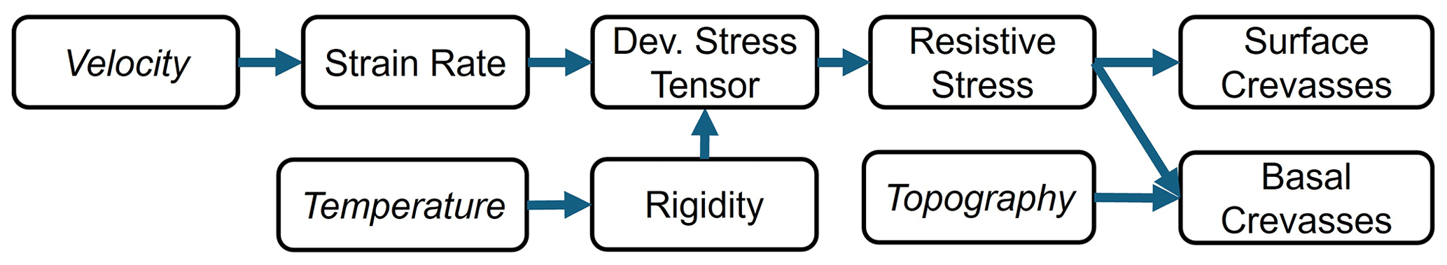
Figure 2Flowchart showing the steps to calculate surface crevasse depths and basal crevasse heights from remote sensing velocity products. Italicized text indicates inputs from remote sensing products.
As satellite-derived or stake-derived measurements of strain rate yield only the surface value, we will be making the assumption that velocity and thus strain rate are constant with depth, making the vertical shear stress terms (σxz, σyz) zero. This is the assumption of the shallow shelf approximation (MacAyeal, 1989), which holds for ice shelves but is also a good approximation for grounded ice with high amounts of basal slip including at tidewater glaciers near the terminus (e.g., Cuffey and Paterson, 2010, p. 495; Lüthi et al., 2002; van der Veen et al., 2011), in ice streams (e.g., Echelmeyer et al., 1994; MacAyeal, 1989), and even at some of Greenland's slower-moving margins (Maier et al., 2019).
In the subsequent sections considering these calculation choices and the rest of this study, we use the following notation throughout except when noted otherwise. Capital X, Y, and Z subscripts indicate directions aligned with a global, arbitrary coordinate system with X and Y being the surface planar directions. Lower case x, y, and z subscripts indicate the local crevasse-perpendicular, crevasse-parallel, and vertical directions, respectively. The local x and y will usually differ from the global X and Y, as shown in Fig. 3, whereas Z and z will be equivalent. The flow direction is indicated by the subscript “flow dir”. Figure 3 shows these coordinate systems. Also, maximum and minimum principal stresses or strain rates from the surface terms receive subscripts of 1 and 2, respectively. (The true minimum principal term would sometimes be the vertical direction.) τij and σij are used to denote components of the deviatoric stress tensor and Cauchy stress tensor, respectively. Finally, Rxx is the resistive stress perpendicular to the crevasse, which is the only direction of resistive stress needed.
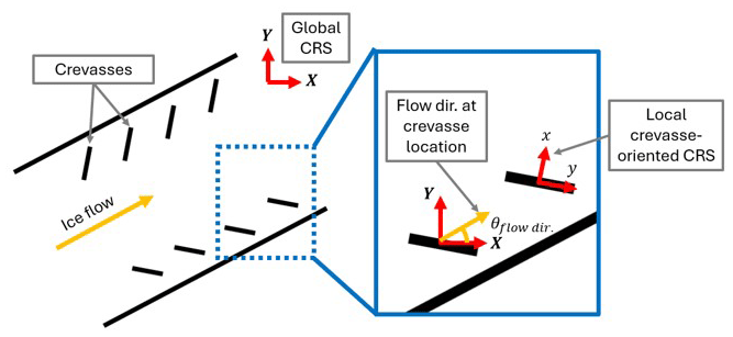
Figure 3Diagram showing the global coordinate reference system (CRS), local crevasse-aligned CRS, and local flow direction angle relative to the global CRS.
2.5.2 Effective strain rate
The first determination in calculating stresses we consider is the calculation of the effective strain rate. Some implementations of crevasse depth calculations neglect effective strain rate and apply Glen's flow law (Glen, 1952) in a single dimension to determine the deviatoric stress in the crevasse-perpendicular direction, τxx, as
where B is ice rigidity (. Other studies use Nye's generalization of Glen's flow law (Nye, 1953), which accounts for the softening of ice from flow in multiple directions and gives each deviatoric stress component, τij, from the corresponding strain rate component, , as
where is the effective strain rate,
Given the shallow shelf approximation, the and terms will both be zero. Most remote sensing velocity products include only horizontal (or planar) velocities, so studies using these products are only able to directly calculate the planar strain rate components (). From incompressibility, the divergence of velocity is zero. This means that the vertical strain rate is given by
In the testing of the crevasse depth calving law by Amaral et al. (2020), the effective strain rate is calculated without the vertical strain rate. The same resulting value in our notation with the global coordinate systems comes from
which we define as the planar effective strain rate, . The implication of assuming no vertical strain rate is a change of ice density for a moving parcel of ice of rate
Neglecting the vertical strain rate is incorrect when considering stress prior to crevasse formation, but it could be argued that incompressibility no longer applies once crevasses exist. We will refer to the effective strain that includes the vertical strain from continuity as the full effective strain rate and consider crevasse depths calculated without the effective strain rate, with the planar effective strain rate, and with the full effective strain rate.
2.5.3 Stress direction
Studies including crevasse depth calculations in three dimensions must select a stress direction. In their tests of the crevasse depth calving law, Amaral et al. (2020) used the maximum principal stress direction, while Choi et al. (2018) and Lai et al. (2020) tested with both the maximum principal and flow direction stresses. Van der Veen (1999) found that crevasses generally open nearly perpendicular to the maximum principal stress direction. We will show representative calculations and crevasse depth maps with each direction. The flow direction, θflow dir., is given by
where VY and VX are the y and x components of velocity in the global coordinate system. The normal, deviatoric stress in the flow direction can be calculated as
The maximum and minimum principal deviatoric stresses are given by
which is the equation for the eigenvalues of the surface terms (a two-by-two matrix). Note that the vertical deviatoric stress will often be the true maximum or minimum principal deviatoric stress. If the surface terms are compressive, the vertical stress will be the true maximum principal stress and horizontal plane fracturing would be predicted. When the surface terms are tensile, the vertical term will be compressive and would be the minimum principal deviatoric stress. Throughout this study, maximum and minimum principal deviatoric stresses, τ1 and τ2, will always refer to surface components. The principal stresses are invariants with coordinate transformation, while the flow direction stress is not. There is no difference between rotating to a direction before or after calculating effective strain rate and deviatoric stress components, assuming that ice rheology is isotropic (the effective strain rate is an invariant).
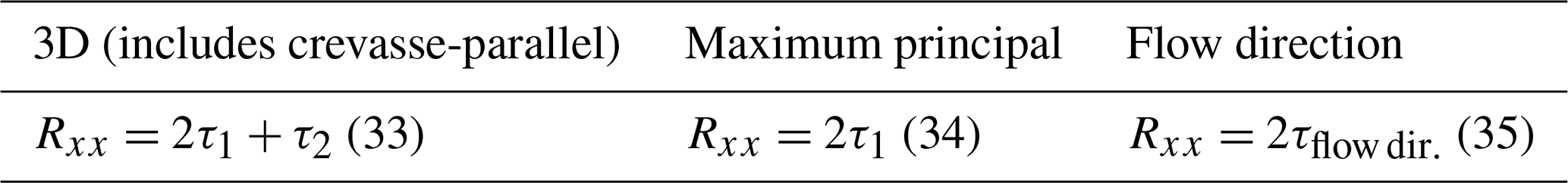
Table 1Equations for resistive stress assuming crevasse formation in the maximum principal and flow directions with and without the crevasse-parallel deviatoric stress.
2.5.4 Crevasse-parallel stress term in the resistive stress
From van der Veen (2013), the resistive stress, Rxx, is defined as the full stress minus the lithostatic pressure and is given by
when bridging stress is neglected in accordance with the shallow shelf approximation (MacAyeal, 1989). For the zero stress approximation, a derivation that yields the use of the resistive stress is as follows. The definitions of the normal, planar, deviatoric stress terms, τxx and τyy, are
where σ terms are Cauchy stress components. These equations combine to give
The vertical full stress component is assumed to come only from ice lithostatic pressure and water pressure. For vertical stress at the crack tip for surface and basal crevasses, respectively, this gives
where (as before) ρi is ice density, ρmw is meltwater density, ρpw is proglacial water density, H is ice thickness, D is proglacial water depth, g is the gravitational acceleration, ds is surface crevasse depth, dmw is the height of meltwater in surface crevasses, and db is basal crevasse height. Equations (29) and (30) can be substituted into Eq. (28) to find the full stress at the crack tip as a function of surface crevasse depth and basal crevasse height. The zero stress approximation predicts crevasse tips where σxx=0, which will give the transition point between tension and compression. This yields the following equations for surface and basal crevasse sizes, respectively:
Note that when aligned such that τxx is the maximum principal deviatoric stress (τ1), τyy will be the minimum principal deviatoric stress (τ2) again considering only the surface terms. The physical explanation for the lateral term is that the full stress in the longitudinal direction must be higher to create the same longitudinal deviatoric stress if there is also a tensile lateral stress.
Studies using two-dimensional flowline models like Nick et al. (2010) inherently do not use the crevasse-parallel, τyy, term. However, for studies working with plan-view ice sheet models or remote sensing products, this term has been included (Amaral et al., 2020) or neglected (Choi et al., 2018; Lai et al., 2020; Sun et al., 2017). The resulting resistive stress, Rxx, terms are shown in Table 1. We only consider the crevasse-parallel stress term when using the maximum principal direction stress, as we found no examples in the literature that considered it with flow direction stress.
Finally, several studies have used a deviatoric stress component (either maximum principal stress or flow direction) rather than the resistive stress in implementations of both the zero stress approximation and LEFM (Sun et al., 2017; Choi et al., 2018; Enderlin and Bartholomaus, 2020). Use of deviatoric stress is not consistent with underlying ice failure assumptions in these crevasse depth theories and will underpredict crevasse sizes by a factor of 2 for the zero stress approximation (with constant density and temperature) and around 2 for LEFM compared to correctly using resistive stresses. The results for such calculations will not be shown.
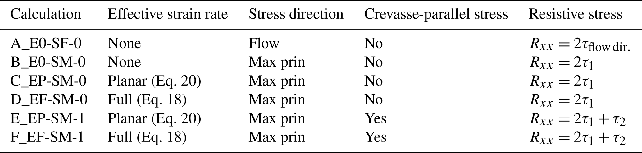
We calculate crevasse depths with a subset of all possible combinations of effective strain rate, stress direction, and resistive stress calculations discussed above. The stress calculation versions being tested are given in Table 2 and will be referred to by the names listed there throughout the rest of this study. Only one flow direction stress calculation is included, as the studies where the selection is significant (plan view) tend to use the maximum principal stress direction. Also, as noted, van der Veen (1999) showed that crevasses tend to align (with some variation) with the maximum principal stress direction. Table 2 does not contain all possible permutations but instead only several that occur in the literature. For example, there are no cases where the crevasse-parallel stress is considered (low simplification) but the effective strain rate is neglected (high simplification). The impact of the selection will be shown through idealized deformation state test cases, plots of predicted crevasse penetration on real ice shelves, and modeling ice shelf velocities with crevasse penetration as damage.
Table 2Summary of effective strain rate, stress direction, and crevasse-parallel deviatoric stress used for each calculation considered as well as the corresponding resistive stress equations. The calculation names indicate the versions of individual calculation steps used. Effective strain rate may be (E0) not used, (EP) taken as planar effective strain rate, or (EF) taken as full effective strain rate. The stress direction may be (SM) maximum principal or (SF) flow. Crevasse-parallel stress may be (0) not used or (1) used.
3.1 Idealized deformation state test cases
Before calculating crevasse depths on real shelves, it is useful to review the expected differences between calculations for idealized strain rate states of biaxially spreading flow, uniaxial extension, and pure shear. Biaxial spreading occurs for unconfined ice tongues and, to a lower extent, areas of spreading flow via non-parallel shear margins, such as on the Scar Inlet ice shelf. Uniaxial extension occurs in the center of glaciers in fjords or shelves with parallel shear margins such as the Pine Island Glacier shelf. Pure shear is approached in shear margins.
3.2 Ice shelf crevasse penetration maps
3.2.1 Crevasse penetration workflow
We calculate crevasse penetration maps for several Antarctic ice shelves. Crevasse penetration is the ratio of crevassed ice thickness to the total thickness:
To do this, we use a workflow described by the flowchart in Fig. 2. The calculation of the deviatoric stress tensor from strain rates and the calculation of the resistive stress from the deviatoric components are varied for each version being tested. The surface topography comes from the reference elevation map of Antarctica (REMA) mosaic product (Howat et al., 2019) as included in BedMachine (Morlighem et al., 2020; Morlighem, 2022). Velocity comes from the ITS_LIVE annual mosaic products (Gardner et al., 2018, 2022) and MEaSUREs multiyear averaged products (Rignot et al., 2022). As the REMA mean year is 2015, velocities from 2015 are used except where a different time period gives better matching ice extents between the topography and velocity data.
Strain rates are calculated from velocity with second-order accurate central differences and no filtering. Strain rate maps are available in the Supplement (Fig. S1). Surface crevasse depths are calculated with constant rigidity corresponding to the surface temperature from Comiso (2000), and basal crevasse heights are calculated with constant rigidity corresponding to the saltwater freezing temperature, −2 °C. This may be a reasonable assumption in areas with marine ice or if crevasses change in size slowly as they advect to locations with different stresses, allowing warming. If stress increases suddenly, however, such that the crevasse grows immediately to a larger size without its tip reaching −2 °C, the actual crevasse penetration will be larger than what is modeled. Ice rigidity, B, as a function of temperature comes from the Cuffey and Paterson (2010) rheology.
An important note for working from remote sensing velocity products on ice shelves is that the calculated stress will be impacted by the presence of crevasses themselves (Surawy-Stepney et al., 2023), particularly as basal crevasses may penetrate a large fraction of the total thickness (Luckman et al., 2012; McGrath et al., 2012). Rifts are the extreme case where complete failure has occurred and a calculation of complete crevasse penetration would be virtually guaranteed by the high strain rate and low thickness present because of the rift itself, even though the calculated stress does not exist in the discontinuous material making up the rift. Using a term from plasticity, the stress calculated is a trial stress: the stress that would exist if the material had the strength to sustain it without failure. (In plasticity, the trial stress is the elastic stress that would exist if the yield strength of the material were not exceeded; Shabana, 2018, p. 287). Where ice is at least partially continuous (crevasses exist but do not penetrate full thickness), the crevasse is predicted through the fraction of ice that, if it were continuous, has tensile (>0) Cauchy stress assuming, for the basal crevasse, the presence of ocean water pressure. Considering the effect of horizontal force balance (Buck, 2023), it is also possible that the stress being measured is nearer to the updated ligament stress because of crevasses (Rxx,1) than the stress that would have existed in the thicker cross section (assumed to be unchanged by the zero stress approximation) to maintain the same force (Rxx,0). In any case, to avoid drawing attention to trivial results in rifts, we mask out regions with thickness below 150 m in the subsequent plots of crevasse penetration. We also produce crevasse penetration maps with an n=4 rheology (Goldsby and Kohlstedt, 2001; Millstein et al., 2022) as well as with horizontal force balance in the Supplement.
3.2.2 Ice shelf selection
We compare the predicted crevasse penetration from each calculation on two ice shelves: the Scar Inlet shelf and the Pine Island Glacier shelf. We study shelves in particular because, in the subsequent modeling component of the study, floating ice removes the confounding effect of basal drag and may have bulk rheology that is strongly impacted by the presence of large basal crevasses. The Scar Inlet ice shelf was the southern portion of the larger Larsen B shelf that collapsed in 2002 and is also sometimes referred to as the Remnant Larsen B (e.g., Khazendar et al., 2015). The Scar Inlet was selected as it has both shear margins and spreading flow. These features highlight the difference between calculations in different strain rate states. Shear margins became a focus after finding larger differences in predicted crevasse penetration in those of the Scar Inlet. This led to studying the Pine Island Glacier ice shelf as it also has well-defined shear margins, one of which broke up around 2018 (Lhermitte et al., 2020).
3.3 Testing with velocity prediction using crevasse penetration as damage
Some checking of crevasse depth calculations can be done by assessing whether the results are realistic. For example, some calculations will predict shear margins that have basal crevasses alone penetrating full thickness, which is physically inconsistent with an observation of an intact shear margin. For calculations that yield plausible results (E_EP-SM-1 and F_EF-SM-1), validation would require measurement of crevasse depths and detailed knowledge of ice temperature, which are rarely (if ever) available. In an attempt to get around this problem, we use crevasse penetration (Eq. 36) as damage, as proposed in Sun et al. (2017). The damage field is used to model velocity in the Ice-sheet and Sea-level System Model (ISSM) (Larour et al., 2012), allowing for comparison to the observed velocity field. ISSM is run with the shallow shelf approximation (MacAyeal, 1989), which cannot represent individual fractures but can be used to study the bulk rheology impact of crevasses.
We take crevasse penetration calculated with constant surface temperature for surface crevasses and constant −2 °C temperature for basal crevasses as damage. We assume that the depth-averaged rigidity that damage is applied to is constant across the shelf and iteratively tune this value for the lowest mean absolute velocity misfit across the nodes. This method decouples the temperature for crevasses from the temperature profile for depth-averaged rigidity, which is likely not physically consistent. Despite this, the method allows for a pattern of damage based on crevasse penetration for the various stress calculations to be tested for its ability to recreate the observed velocity pattern. To have reference points, we also calculate velocities with no damage and with inverted damage. For the undamaged velocity predictions, temperature again must be assumed. Without damage, a falsely cold temperature will yield higher misfit than the real temperature. We intentionally select a temperature profile that is likely warmer than the fast-flowing portions of the shelves, which is shown as Fig. S5 in the Supplement. This is a conservative choice to ensure that the crevasse-based damage is not made to look more successful than it really is by overly high error from the undamaged predictions. Inversions were initialized with 40 % damage, as done in Borstad et al. (2016). Like noted in Borstad et al. (2016), we found that the success of the inversion in matching velocity was not very sensitive to this selection of 40 % (we tested 30 % to 70 %). Inversions used only velocity misfit (mean squared error) as the cost function except when including small coefficients for log velocity misfit, and regularization terms helped find a solution with lower velocity misfit. The inversion cost function is provided in Sect. S9. The depth-averaged rigidity assumed for the initial rheology in the inversion was set to a tuned value from calculation F_EF-SM-1 to have the same bounds on the resulting rigidity; maximum damage was set to 90 % as rigidity nearing zero causes model instability (Borstad et al., 2016).
This analysis requires imperfect assumptions including the noted temperature assumptions regarding both the crevasse depth and depth-averaged rigidity, which will impact predicted crevasse penetration (Coffey et al., 2024). We analyze the impact of the flow law exponent by considering an n=4 flow law (Goldsby and Kohlstedt, 2001; Millstein et al., 2022) in the Supplement; our findings are insensitive to the selection. Rifts are included in the domain and therefore treated as continuous features. Finally, damage, calculated both from crevasse penetration and with inversion, is implemented assuming isotropy due to model capability. The reduction in load-bearing area from crevasses would be expected to be directional and anisotropic damage laws have been shown to better capture tabular iceberg calving (Huth et al., 2021). Despite these assumptions, this workflow allows us to test velocity fields produced by damage from each calculation's crevasse penetrations, giving a method of testing predicted crevasse fields' connection to bulk rheology. We also test crevasse penetration calculated with horizontal force balance using this workflow, which yielded mixed results across the two shelves considered (Sect. S7 in the Supplement).
The ice shelves selected for our analysis are small shelves that show high amounts of crevasse penetration, which makes it more likely that damage, not temperature, drives the pattern of rheology so that the error in the total rigidity field from assuming constant temperature is lessened. The shelves used to compare predicted crevasse penetration (Scar Inlet and Pine Island) meet these criteria, as do the Brunt/Stancomb–Wills, Larsen C, and Fimbul ice shelves.
4.1 Crevasse depths for representative strain states
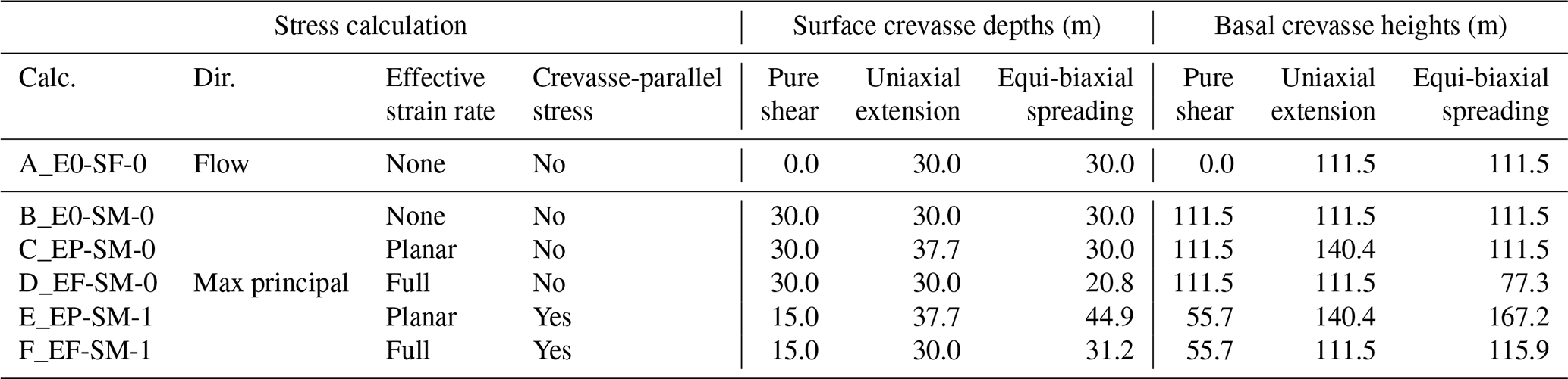
As noted in Sect. 3.1, pure shear, uniaxial extension, and biaxial spreading are simplified strain rate states that are representative of shear margins, centerlines of confined glaciers, and unconfined ice fronts, respectively. To compare the stress calculations in these idealized flow types, the same magnitude is used for each strain rate component (, ), which are assumed to be constant through thickness. The strain rate component magnitude, 0.012 yr−1, corresponds approximately to the center of flow near the terminus of the Scar Inlet ice shelf, which has high and spreading strain rates. Table 3 shows surface and basal crevasse sizes for these three representative strain rate states. For pure shear, the flow direction stress (calculation A_E0-SF-0) predicts no crevasse depth as the flow direction normal stress is zero. The differences from effective strain rate and crevasse-parallel stress are better shown graphically and are discussed with Fig. 4 next. The remaining takeaway from this table is that, even with the warmer ice temperature assumed, basal crevasses are nearly 4 times larger than surface crevasses and will make up most of the total crevasse penetration.
Table 3Surface and basal crevasses with each stress calculation for representative strain rates for equi-biaxial spreading ( yr−1, yr−1, yr−1), uniaxial extension ( yr−1, yr−1, yr−1), and pure shear ( yr−1, yr−1, yr−1). The flow direction is in this example (breaking notation). Ice rigidity corresponds to −18 °C for surface crevasses and −2 °C for basal crevasses. Strain rate is assumed to be constant through thickness.
For all crevasse depth calculations that assume the crevasse forms perpendicular to the maximum principal stress direction (calculations B_E0-SM-0 to F_EF-SM-1), the difference in crevasse depths can be shown as a function of the ratio of minimum principal strain (of the surface terms) to maximum principal strain rate, , with a constant maximum principal strain rate, . When this ratio is −2.0, all longitudinal extension comes from compressive lateral stress such that the longitudinal resistive stress (when three-dimensional) is zero. A ratio of −1.0 occurs when the surface principal strain rates are equal and opposite, as is the case for a pure-shear shear margin when a stress rotation 45° from flow is performed. is 0.0 for longitudinal extension as in the center of flow where shear margins are parallel. is +1.0 for a fully unconfined ice tongue spreading equally in both surface directions. Figure 4 a to d show velocity magnitude and the value of across the Scar Inlet and Pine Island Glacier ice shelves. Values of near −2 occur where the glacier inlets into the Scar Inlet shelf merge (Fig. 4c). As expected, values of around −1 can be seen in the shearing zones of both shelves. Pine Island has near zero in the center of flow (with increasing local variation near the front), while the Scar Inlet has higher values toward the front as lateral spreading occurs from the opening shear margins. Predicted basal crevasse depth for a constant maximum principal strain rate as a function of is shown in Fig. 4e. The values for a basal crevasse are presented, but the ratios of depths between calculations will be identical to those of dry surface crevasse calculations so long as depth-variable temperature and density are neglected. For example, surface crevasse depth predictions for a strain rate state corresponding to −1 on the x axis with calculations B_E0-SM-1, C_EP-SM-0, and D_EF-SM-0 will still yield a depth twice that of calculations E_EP-SM-1 and F_EF-SM-1.
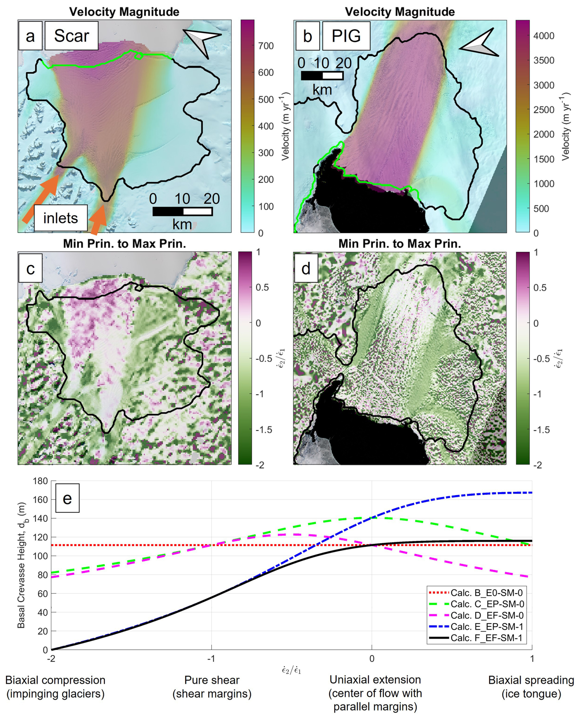
Figure 4(a) Surface velocity (MEaSUREs 2014–2017 – Gardner et al., 2022, 2018) of the Scar Inlet ice shelf, (b) surface velocity (ITS_LIVE 2015 – Rignot et al., 2022) of the Pine Island Glacier ice shelf, (c) ratio of minimum to maximum principal surface strain rates at Scar Inlet, (d) the same at Pine Island, and (e) basal crevasse heights for each stress calculation using maximum principal direction stresses (all except calculation A_E0-SF-0) as a function of the ratio of minimum to maximum principal strain rate. The maximum principal strain rate, , is held constant as 0.0117 yr−1 and the minimum principal strain rate, , ranges from −0.0234 to 0.0117 yr−1. On the x axis, −2 occurs when all longitudinal extension is caused by lateral compression, −1 is a state of pure shear, 0 is longitudinal extension, and +1 is equi-biaxial spreading. These points are labeled as descriptions (example location). The black line in (a), (b), (c), and (d) is shelf extent, and the green line in (a) and (b) is the calving front.
The maximum principal stress direction with no effective strain rate calculation (calculation B_E0-SM-0) predicts the same crevasse height regardless of minimum principal strain rate. The calculations including crevasse-parallel deviatoric stress (calculation E_EP-SM-1 and F_EF-SM-1) reduce the crevasse depth when is negative because there will be a negative minimum principal deviatoric stress, τ2, counteracting the maximum principal (τ1) in the resistive stress (). Because the pure shear state () has surface strain rates that are equal in magnitude but opposite in sign, mass conservation is met with no vertical strain rate. This causes the pure-shear crevasse depths to be independent of the selection of planar or full effective strain rate, explaining the equivalency of calculations E_EP-SM-1 and F_EF-SM-1 as well as calculations C_EP-SM-0 and D_EF-SM-0. As the minimum principal strain rate becomes more positive, the vertical strain rate magnitude grows, increasing the effective strain rate when continuity is respected. This reduces the stress from the same value of maximum principal strain rate, explaining the smaller crevasse depths from the full effective strain rate calculations (D_EF-SM-0 and F_EF-SM-1) compared to their planar effective strain rate counterparts (C_EP-SM-0 and E_EP-SM-1) when moving towards the right side of the plot. For positive values of minimum principal strain rate, the simple calculation without effective strain rate (calculation B_E0-SM-0) is nearly equivalent to the most physically based calculation that includes effective strain rate and crevasse-parallel deviatoric stress (calculation F_EF-SM-1). For calculation F_EF-SM-1, as the minimum principal strain rate increases, the increase in effective strain rate reduces stress in the maximum principal direction. This effect is apparently canceled by the growing minimum principal stress term to explain the nearly constant value of calculation F_EF-SM-1 from 0.0 to 1.0 on the x axis.
4.2 Crevasse penetration on the Scar Inlet ice shelf
Figure 5 provides the crevasse penetration () for the Scar Inlet ice shelf with each stress calculation listed in Table 2. The Scar Inlet was selected as it includes both shear margins (approximately pure shear) and spreading flow, which, as our idealized test case shows, will highlight where differences between calculations occur (Table 3 and Fig. 4e). Results over rifts have been masked out using a 150 m thickness threshold to avoid highlighting the trivial result of full crevasse penetration. The calculations using the maximum principal direction but neglecting crevasse-parallel deviatoric stress (calculations B_E0-SM-0, C_EP-SM-0, and D_EF-SM-0) appear similar and are characterized by wide zones of full crevasse penetration in the shear margins. The flow direction calculation (A_E0-SF-0) and the two maximum principal direction calculations that use the full resistive stress (calculations E_EP-SM-1 and F_EF-SM-1) show similar results to one another. Calculation A_E0-SF-0, however, does predict more zones of no damage where the flow direction stress components are not tensile.
Next, we compare crevasse penetration predicted by each calculation against that of calculation F_EF-SM-1. These differences in crevasse penetration are shown in Fig. 6. In the fast-flowing center, particularly near the terminus, calculation E_EP-SM-1 predicts higher crevasse penetration than calculation F_EF-SM-1. This is likely because of increased lateral spread between the diverging, non-parallel shear margins causing the crevasse-parallel deviatoric stress to increase relative to the maximum principal (crevasse-perpendicular) stress. This corresponds to moving toward the right side of the Fig. 4e plot. There is also a large difference in crevasse penetration between calculation F_EF-SM-1 and the calculations in the max principal direction that do not include crevasse-parallel stress (calculations B_E0-SM-0, C_EP-SM-0, and D_EF-SM-0) in the region between the two inlets. As noted, calculations B_E0-SM-0, C_EP-SM-0, and D_EF-SM-0 predict higher crevasse penetrations because they neglect the compressive lateral stress in this region, which results from the converging flow. This causes a negative minimum principal stress term and corresponds to the left side of Fig. 4e. Calculation A_E0-SF-0 predicts lower crevasse penetration in the glacier inlets themselves. This is because lateral spreading is occurring faster than longitudinal spreading such that the maximum principal stress direction is rotated approximately 90° from the flow direction. In the rest of the fast-flowing center region closer to the front, the flow direction and maximum principal directions more closely align such that calculation A_E0-SF-0 is nearer to calculation F_EF-SM-1.
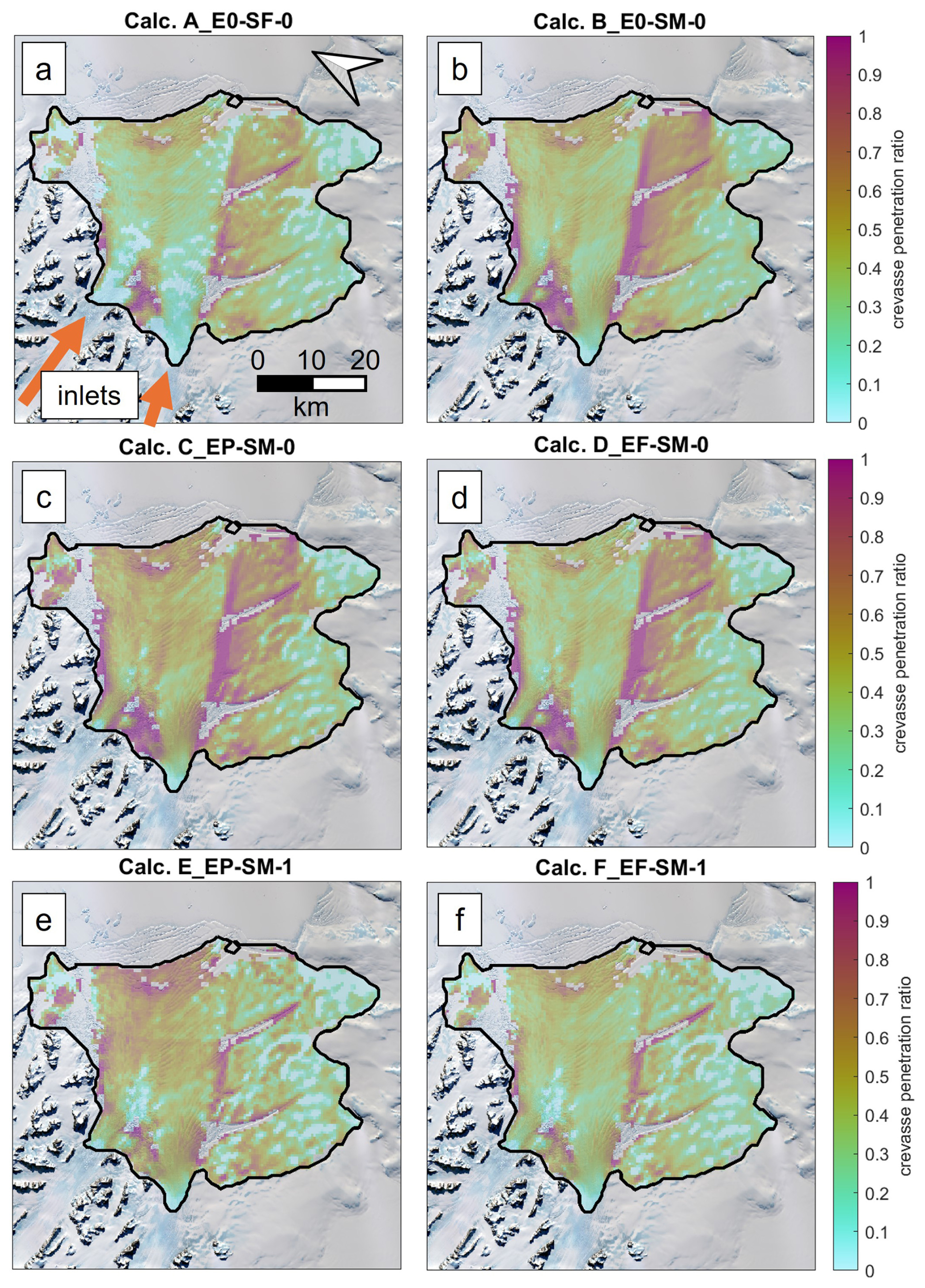
Figure 5Crevasse penetration at the Scar Inlet ice shelf with (a) calculation A_E0-SF-0, (b) calculation B_E0-SM-0, (c) calculation C_EP-SM-0, (d) calculation D_EF-SM-0, (e) calculation E_EP-SM-1, and (f) calculation F_EF-SM-1 resistive stress versions overlaid on satellite imagery from October 2014 (Landsat-8 image courtesy of the US Geological Survey). The glacier inlets into the Scar Inlet shelf (Flask and Lepperd glaciers) are shown in (a). Crevasse penetration is not shown for ice less than 150 m thick to mask out rifts. Ice flow direction is approximately from image bottom to top, as shown with orange arrows in panel (a).
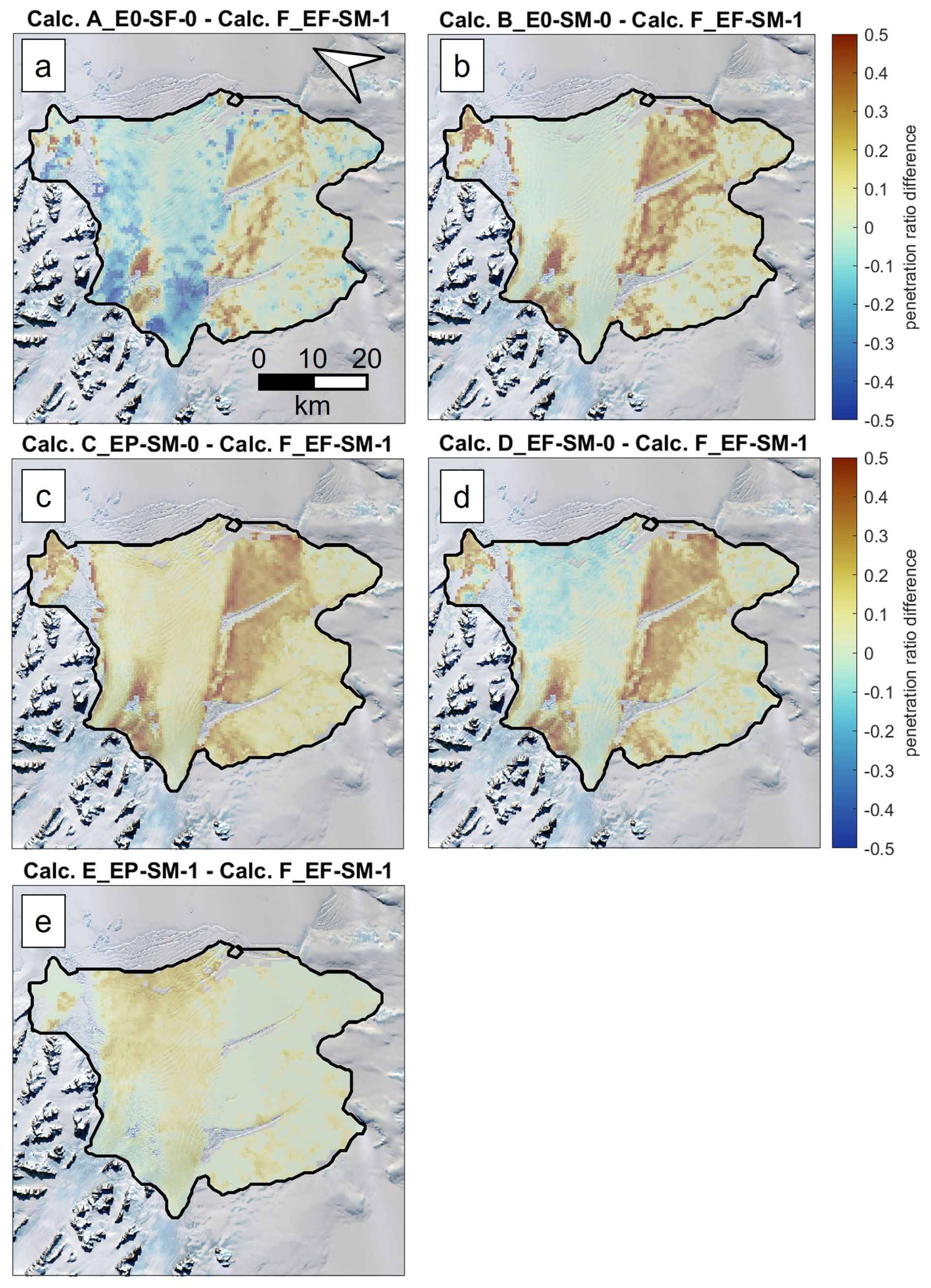
Figure 6Difference from calculation F_EF-SM-1 crevasse penetration for (a) calculation A_E0-SF-0, (b) calculation B_E0-SM-0, (c) calculation C_EP-SM-0, (d) calculation D_EF-SM-0, and (e) calculation E_EP-SM-1 at the Scar Inlet ice shelf.
4.3 Crevasse penetration in ice shelf shear margins
Next, we use cross-section plots to examine differences in crevasse penetration across shear margins. Figure 7 shows the observed surface velocity, thickness, minimum to maximum principal strain rate ratio, and crevasse penetration on a transect across the fast-flowing portion of the Scar Inlet shelf. The crevasse penetration plot (Fig. 7e) again shows a large difference between the maximum principal stress calculations that do and do not include the crevasse-parallel deviatoric stress in the resistive stress when is less than −0.5. The calculations including crevasse-parallel stress (E_EP-SM-1 and F_EF-SM-1) predict high but not total crevasse penetration in both shear margins, whereas all maximum principal direction calculations neglecting the crevasse-parallel deviatoric stress (B_E0-SM-0, C_EP-SM-0, D_EF-SM-0) predict complete penetration. Interestingly, the flow direction calculation (A_E0-SF-0) predicts less crevasse penetration in the northwestern shear margin but more in the southeastern shear margin relative to calculations E_EP-SM-1 and F_EF-SM-1. Misalignment between the flow and principal direction would reduce calculation A_E0-SF-0's crevasse penetration, while the lack of crevasse-parallel stress may add penetration should the flow direction not fully misalign. The smooth velocity profile (Fig. 7c) through the shear margins and appearance of continuous ice in the shear margins away from the rifts (Fig. 7b) suggest that full crevasse penetration should not be predicted. (The Brunt/Stancomb–Wills shelf has examples of fully failed (rift) shear margins with a discontinuous velocity profile, and a figure equivalent to Fig. 7 for the Brunt is available as Fig. S2 in the Supplement.) This suggests the calculations that use the maximum principal direction but do not include the crevasse-parallel deviatoric stress (calculations B_E0-SM-0, C_EP-SM-0, and D_EF-SM-0) overpredict crevasse depths. The surface elevation (Fig. 7b) of the southeastern shear margin shows visible features oriented 45° from flow, which may suggest crevasses forming approximately perpendicular to the maximum principal stress.
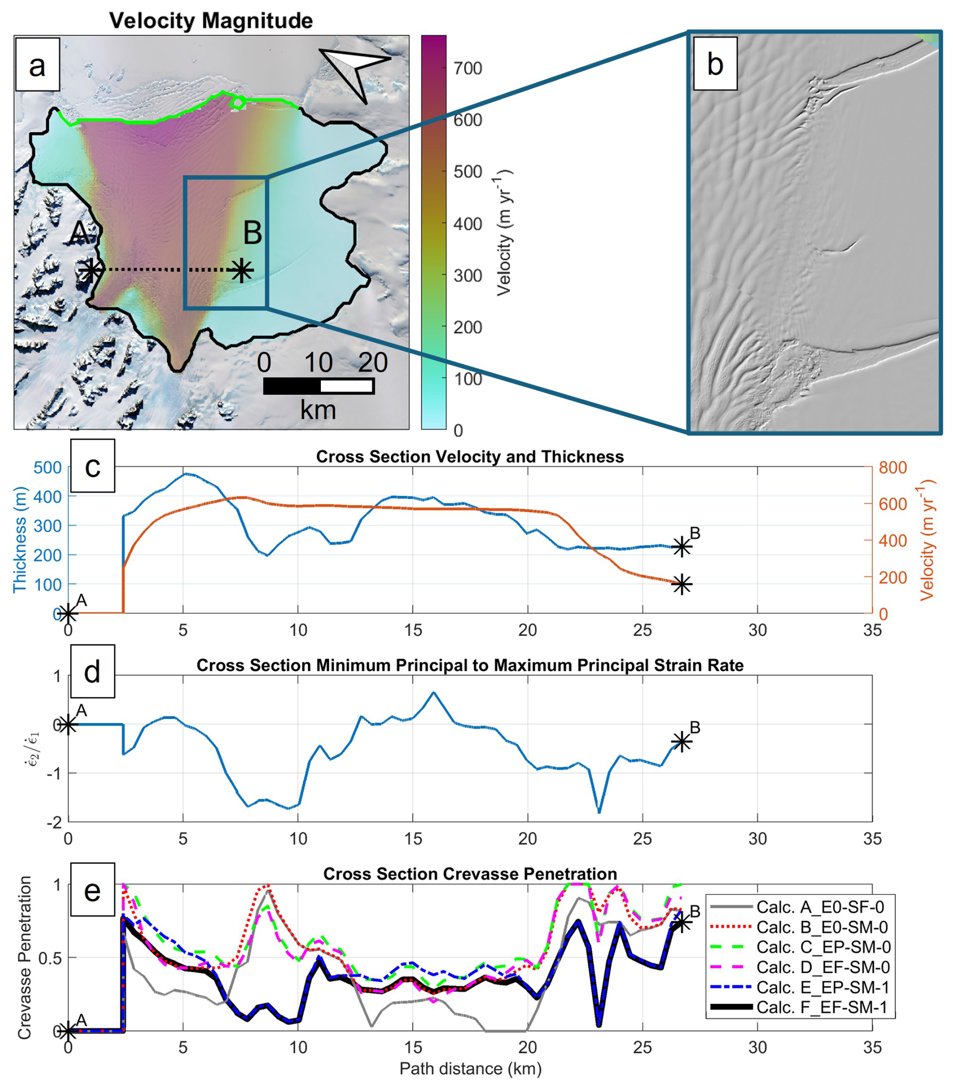
Figure 7(a) Observed velocity map (MEaSUREs 2014–2017 – Gardner et al., 2022, 2018) with cross-section location, (b) 2015 hillshade REMA (Howat et al., 2019) snapshot of the shear margin between rifts, (c) cross-section velocity and thickness, (d) cross-section minimum to maximum principal strain rate ratio, and (e) cross-section crevasse penetration at the Scar Inlet ice shelf.
With the focus on differing crevasse penetration predictions in shear margins, we next consider the Pine Island Glacier shelf. It again shows full penetration in its shear margins with all versions of crevasse depth calculations that do not include the effect of the crevasse-parallel deviatoric stress. Figure 8 shows this for calculation C_EP-SM-0, which yields similar results to the other calculations without the minimum principal deviatoric stress, τyy. Calculation F_EF-SM-1 again predicts significant but not complete crevasse penetration throughout the shear margins (Figs. 8b and 9e).
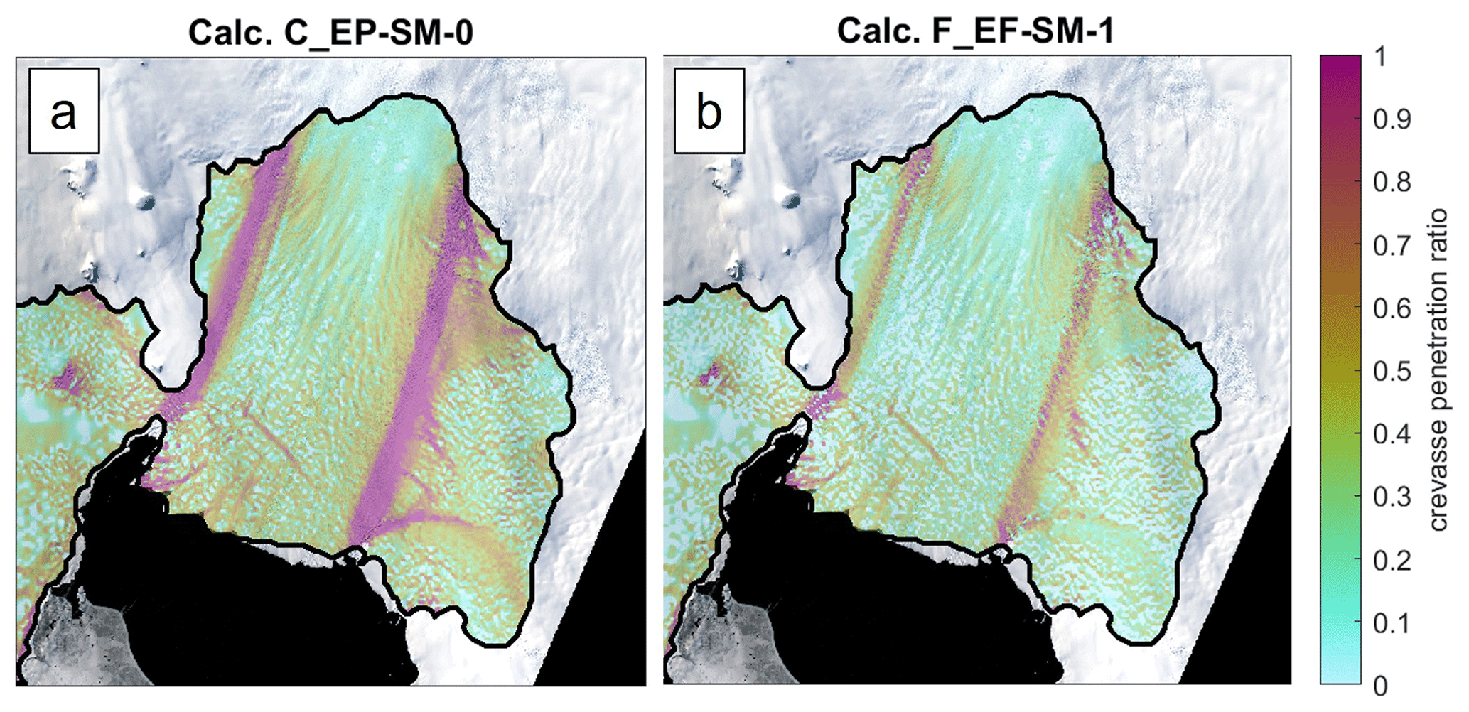
Figure 8Crevasse penetration ratio on Pine Island Glacier ice shelf with (a) calculation C_EP-SM-0 and (b) calculation F_EF-SM-1. Crevasse penetration is overlaid on satellite imagery from November 2014 (Landsat-8 image courtesy of the US Geological Survey). Ice flow direction is approximately from the image top right to bottom left.
Pine Island's south shear margin failed in some regions in 2018, which can be seen in the 2014 and 2018 surface elevation views provided in Fig. 9b. This later collapse suggests that partial crevasse penetration rather than total crevasse penetration prior to 2018 should be predicted, again favoring the use of the crevasse-parallel deviatoric stress term. The flow direction calculation (A_E0-SF-0) predicts no crevasse penetration in the northern shear margin. In the center of flow, differences between the different stress calculations are small (Figs. S2 and S3). This is because, unlike the Scar Inlet, Pine Island has parallel shear margins and thus little lateral spreading in the center of flow. Therefore, the strain rate state in the center of flow corresponds to the center portion of Fig. 4e, where there is less range across the calculations.
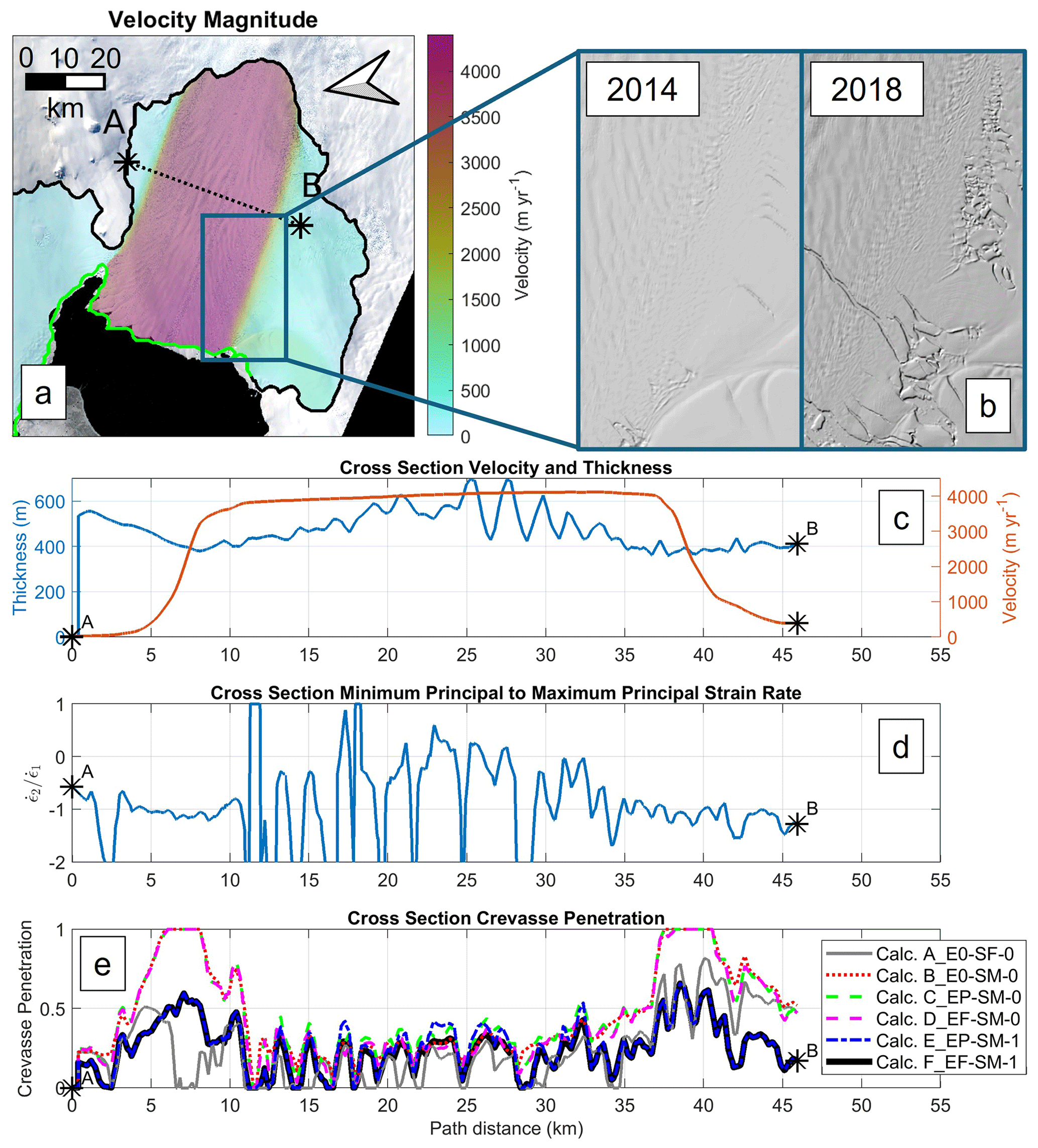
Figure 9(a) Observed velocity (ITS_LIVE 2015 – Rignot et al., 2022) map with cross-section location, (b) hillshade REMA (Howat et al., 2019) views from 2014 and 2018 of the south shear margin, (c) cross-section velocity and thickness, (d) cross-section minimum to maximum principal strain rate ratio, and (e) cross-section crevasse penetration at the Pine Island Glacier ice shelf.
4.4 Velocity comparison results
Velocity predictions were made with crevasse penetration as damage from the two stress calculations that include crevasse-parallel stresses (calculations E_EP-SM-1 and F_EF-SM-1). The maximum principal stress calculations that do not use the crevasse-parallel stress (calculations B_E0-SM-0, C_EP-SM-0, and D_EF-SM-0) are not included, as they all yield fully failed shear margins for Pine Island Glacier's shelf and the Scar Inlet. In these locations, the modeled velocity would fully depend on the selection of the maximum allowable damage, which is a user-defined parameter that protects against an element having full damage and therefore zero rigidity. The flow direction stress calculation (A_E0-SF-0) is also not used for similar reasons and because it is not consistent with the observed orientations of crevasses (Sect. 4.3).
The mean average nodal velocity misfits for damage calculated with calculations E_EP-SM-1 and F_EF-SM-1 as well as with no damage and inverted damage are shown in Fig. 10a. As noted in Sect. 3.3, a spatially constant temperature and thus undamaged rigidity are tuned for the best velocity match averaged across the entire model domain. Damage from crevasse penetration will control the relative rigidity between regions of the ice shelves. The assumption is that the stress calculation that gives the best modeled velocity performs best in predicting relative crevasse depths between regions of the ice shelf (e.g., center of flow, shear margins, unconfined front). Velocity misfits with no damage and from an inversion are included to contextualize the crevasse-penetration-based velocity misfit values.
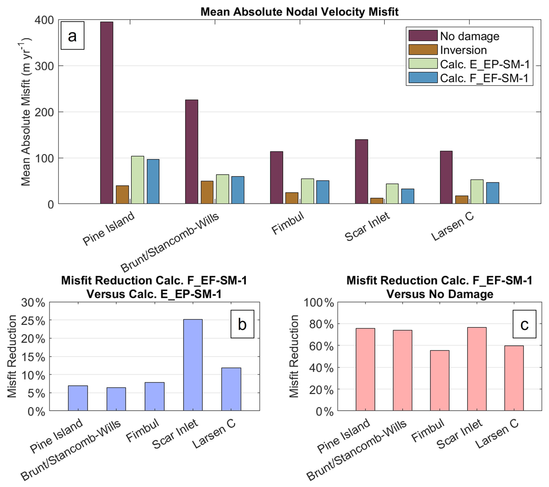
Figure 10(a) Average nodal velocity misfit with no damage, inverted damage, damage from calculation E_EP-SM-1 crevasse penetration, and damage from calculation F_EF-SM-1 crevasse penetration. (b) Misfit reduction percentages with calculation F_EF-SM-1 relative to calculation E_EP-SM-1. (c) Misfit reduction percentages with calculation F_EF-SM-1 relative to no damage.
The primary finding is that calculation F_EF-SM-1 outperforms calculation E_EP-SM-1 at all ice shelves tested by 5 % to 25 % (Fig. 10b), suggesting that including vertical strain rate from continuity yields a damage field more connected to physical crevasse depths. Inversions performed best at all shelves, likely due to their ability to adjust the rigidity field to account for all drivers of bulk rigidity variation (spatial temperature variation, flow law error, and crevasses) rather than just crevasses and bulk temperature. Despite this, setting damage from crevasse penetration and tuning bulk temperature removed most of the misfit relative to no damage and approached the misfit of inversions for some shelves. Bulk temperature is a strong tuning factor because of ice rheology's high sensitivity to temperature; however, we did not need to tune bulk temperature outside of reasonable values. The tuned depth-averaged temperatures are close to the surface temperatures, which is not unreasonable because of the advection of cold ice as can be seen from borehole measurements at the Fimbul and Amery ice shelves (Humbert, 2010; Wang et al., 2022). The tuned temperatures for the Scar Inlet and Pine Island Glacier ice shelves are discussed in Sect. 4.4.1 and 4.4.2. The inversion for the Brunt/Stancomb–Wills only performed better when initialized with the crevasse penetration damage field. Calculation F_EF-SM-1 makes the largest improvements relative to no damage at small shelves with high crevasse penetration (Pine Island, Brunt/Stancomb–Wills, Scar Inlet) as opposed to shelves that are larger (Larsen C) or have less crevasse penetration (Fimbul) as shown by the error reduction percentages in Fig. 10c. Larger shelves may also have more temperature variability that is not being captured, while crevasse penetration may make temperature error more significant in predicting the net bulk rheology.
4.4.1 Scar Inlet velocity predictions
Figure 11 shows the modeled velocity correlation and mapped misfit for calculations E_EP-SM-1 and F_EF-SM-1 at the Scar Inlet ice shelf. The modeled velocity correlation plot for damage from calculation E_EP-SM-1 (Fig. 11a) shows that it predicts excess velocity for the fastest-moving ice near the terminus. This likely stems from the background rigidity tuning, which balanced excess velocity at the terminus with overly slow velocities upstream to minimize the overall misfit. This may indicate that the damage in the spreading flow region approaching the terminus is being overpredicted relative to the shear margins and more confined flow upstream. The full effective strain rate calculation (F_EF-SM-1) predicts smaller crevasses in regions of spreading flow due to increased ice softening from the vertical strain rate term, as seen in Fig. 6e. This fixes the problem of the fast front and slow upstream seen in the planar effective strain rate calculation (E_EP-SM-1) and reduces the average nodal velocity misfit by 25 %, from 43.9 m yr−1 (calculation E_EP-SM-1) to 32.9 m yr−1 (calculation F_EF-SM-1). While local regions with substantial misfit remain, misfit is distributed across observed velocities rather than being concentrated. This provides some evidence that mass conservation should be included in the effective strain calculation even when crevasses are present (calculation F_EF-SM-1 rather than E_EP-SM-1). The modeled velocity maps themselves are available as Fig. S6.
The dense line of points where modeled velocity is slower than observed velocity (below the lower black line in Fig. 11c) corresponds to the blue zones (Fig. 11d) in the slow-moving ice adjacent to shear margins. That the fast-flowing ice is not imparting adequate speed to these areas may suggest the shear margins have been made overly soft. The tuned ice rigidity for calculation F_EF-SM-1 damage corresponds to −19 °C if temperature is constant through thickness ( °). This agrees well with the average surface temperature over the shelf of −17.7 °C from Comiso (2000); the cold bias (being close to the surface rather than basal temperature) likely stems from advection of colder ice from upstream. However, the tuned temperature is colder than thermal-model-derived temperatures in Borstad et al. (2012), which were no colder than approximately −12 °C. This does not significantly alter our findings, however, as we are not testing the ability of crevasse depth to predict the absolute magnitude of damage, only the pattern of damage.
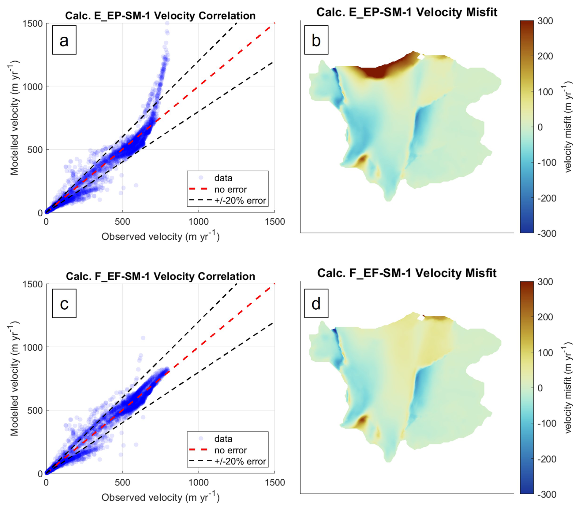
Figure 11Plots of (a) velocity correlation and (b) velocity misfit with calculation E_EP-SM-1 as well as (c) velocity correlation and (d) velocity misfit with calculation F_EF-SM-1 for the Scar Inlet ice shelf. The velocity product used for crevasse penetration calculation and correlation plots is the MEaSUREs 2014–2017 averaged product (Gardner et al., 2018, 2022).
4.4.2 Pine Island Glacier ice shelf velocity predictions
The effect of the full effective strain rate based on mass conservation versus the planar effective strain rate is less significant at the Pine Island Glacier ice shelf, as can be seen in Fig. 12. This is likely due to the parallel shear margins and thus lack of spreading flow that would cause increased stress when the vertical strain rate term is not included in the effective strain rate calculation. Including the full effective strain rate reduces absolute mean nodal misfit by 7 % from 103.5 m yr−1 (calculation E_EP-SM-1) to 96.4 m yr−1 (calculation F_EF-SM-1). Unlike at the Scar Inlet, there is no region or clear spatial pattern in the difference between calculation E_EP-SM-1 and F; the 7 % appears to come from small improvements spread over the whole domain. The tuned background rigidity corresponds to a temperature of −18 °C, which compares well to the average surface temperature from Comiso (2000) of −17.8 °C. The crevasse penetration plots used as damage and their differences are provided in Figs. S3 and S4, and the modeled velocity plots themselves are in Fig. S7.
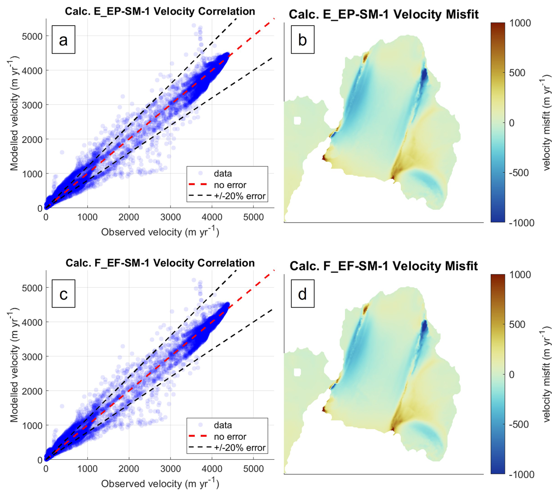
Figure 12Plots of (a) velocity correlation and (b) velocity misfit with calculation E_EP-SM-1 as well as (c) velocity correlation and (d) velocity misfit with calculation F_EF-SM-1 for the Pine Island Glacier ice shelf. The velocity product used for crevasse penetration calculation and correlation is the ITS_LIVE 2015 annual map (Rignot et al., 2022).
5.1 Recommended resistive stress calculation
Our findings support resistive stress calculation F_EF-SM-1 for use in crevasse depth predictions. This recommendation follows analyzing predicted crevasse penetration from six calculations that varied in stress direction, calculation of effective strain rate, and inclusion of crevasse-parallel deviatoric stress in the calculation of resistive stress. Flow direction calculations (e.g. calculation A_E0-SF-0) will not predict crevasses in shear margins in pure shear (Table 3), which was found in some parts of the Pine Island Glacier ice shelf (Fig. 9e). Flow direction stress is also inconsistent with the observation of crevasses forming perpendicular to maximum principal stress in van der Veen (1999) and Colgan et al. (2016) as well as Fig. 7b. Calculations B_E0-SM-0, C_EP-SM-0, and D_EF-SM-0, which use the maximum principal stress direction but neglect the crevasse-parallel deviatoric stress in the three-dimensional resistive stress equation, likely overpredict crevasse penetration in shear margins (Sect. 4.2 and 4.3). These calculations predict complete crevasse penetration throughout most of the shear margins of the Scar Inlet and Pine Island Glacier ice shelves. This result appears inconsistent with the surfaces of these shear margins (Figs. 7b and 9b) and the subsequent failure of one of Pine Island Glacier ice shelf's shear margins (Fig. 9b). The calculations that consider the three-dimensional form of resistive stress (included the crevasse-parallel deviatoric stress), E_EP-SM-1 and F_EF-SM-1, predict crevasses half the size of the calculations using the two-dimensional form (Fig. 4e) in pure shear, fixing the overprediction of crevasse depth in shear margins (Figs. 5 and 8). These calculations (E_EP-SM-1 and F_EF-SM-1) yield identical results in shear margins and similar results in uniaxial extension, but calculation E_EP-SM-1 predicts larger crevasses in biaxial spreading through neglecting the ice softening effect of vertical strain rate (Sect. 4.1). Applying crevasse penetration as damage from these two calculations supports calculation F_EF-SM-1. Calculation F_EF-SM-1 outperforms calculation E_EP-SM-1 in reducing modeled velocity misfit for all shelves, with large improvements at the Scar Inlet and Larsen C (Sect. 4.4). At the Scar Inlet, the improved modeled velocity field of calculation F_EF-SM-1 can be explained by its lower crevasse penetration prediction in biaxially spreading flow. This finding held when implemented with n=4 rheology (Sect. S6). Finally, calculation F_EF-SM-1 is the most physically consistent stress calculation. It can be derived from deviatoric stress equations with the assumptions of continuity, crevasse formation in the maximum principal stress direction, and vertical stress (σzz) coming from only lithostatic pressure and water pressure (Sect. 2.4.3). We would maintain this stress calculation recommendation for crevasse depths calculated with horizontal force balance and LEFM, noting that applying LEFM where the crevasse-parallel stress may take any value violates the plane strain assumption and that our recommendation is based on results using the zero stress approximation. Despite these caveats, applying other stress calculations for LEFM may find high tensile resistive stresses where none exist (Figs. 4e and 7e).
5.2 Classification of stress calculation by study type
As noted throughout the introduction and background, the stress calculation used as input for crevasse depth calculations has varied widely across studies. In some cases, the differences are zero or trivial. For example, the maximum principal stress and flow direction stress in the center of a two-dimensional flowline domain will be equivalent. The calculation may also be limited by measurement method: field studies using stakes or GPS units to directly measure the strain rate across a crevasse may not yield crevasse-parallel strain rates. However, for studies that use planar remote sensing data (Amaral et al., 2020; Lai et al., 2020) or plan-view ice sheet models (Choi et al., 2018; Huth et al., 2021; Sun et al., 2017; Todd et al., 2018), all surface strain terms are available and the selections of effective strain rate, stress direction, and resistive stress equation still differ significantly.
Table 4 shows the stress calculations used by some past studies. It was not always possible to tell with complete certainty which stress calculation was used from the study text; we made a best effort in some cases by working backwards from reported resistive stresses or crevasse depths. Secondly, not all studies fit a category perfectly. Mottram and Benn (2009), for example, directly used the direction perpendicular to the crevasse by measuring strain rate with stakes on either side and therefore did not need to assume that crevasses form perpendicular to flow or maximum principal stress. Studies that used multiple stress calculations are listed in each corresponding cell. Choi et al. (2018) and Lai et al. (2020) both evaluated their results with a flow direction and maximum principal direction calculation. Enderlin and Bartholomaus (2020) used different stress versions for the zero stress approximation and LEFM components of their workflow.
There is a distinction to be made between studies that apply the zero stress approximation for crevasses in ice sheet models. For studies that use full Stokes flow or three-dimensional viscoelastic modeling approaches, the Cauchy stress through thickness is calculated across the domain so the crevasse depth can be determined directly. Studies using the shallow shelf approximation solve for the depth-averaged resistive stress and could bypass these calculations as well. Some modeling-based studies (Choi et al., 2018; Pollard et al., 2015; Sun et al., 2017; Wilner et al., 2023), however, apply the zero stress approximation as a parameterization rather than a physical failure criterion and still calculate a stress for use in crevasse depth equations starting with strain rates or deviatoric stresses. We distinguish studies that apply the zero stress approximation using the modeled stress directly with double asterisks in Table 4.
The 14 studies tabulated use seven distinct stress calculations, with multiple studies selecting calculations A_E0-SF-0, B_E0-SM-0, D_EF-SM-0, and F_EF-SM-1. Four studies (Choi et al., 2018; Enderlin and Bartholomaus, 2020; Hulbe et al., 2016; Sun et al., 2017) use deviatoric rather than resistive stress terms. Only one study that calculates stress from observed strain rates (Scott et al., 2010) uses the most physically consistent calculation (F_EF-SM-1).
Table 4Classification of studies using crevasse depth calculations by the stress calculation method.
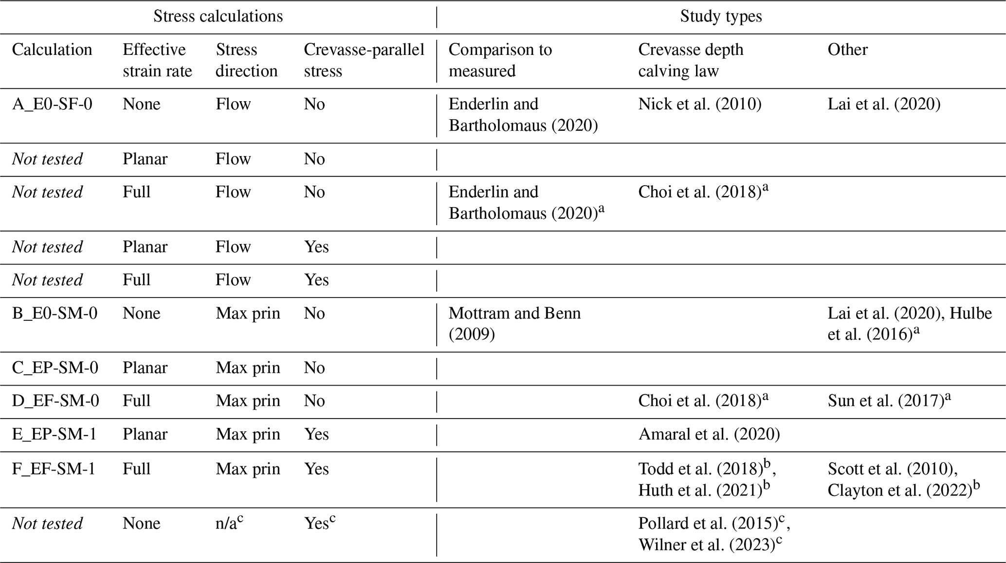
a These studies used (for at least one calculation included in the study) a deviatoric stress term rather than the resistive stress. The predicted crevasse depths would correspond to one-half the values yielded by the calculation classification. The calculation is direction-independent. b These studies use the physical meaning of the zero stress approximation (crevasse extends to where the maximum principal Cauchy stress is zero) in ice sheet models. Where flow is fully viscous and the shallow shelf approximation is a perfect assumption, they would predict identical crevasse sizes to those of calculation F_EF-SM-1. c The calculation developed in Pollard et al. (2015) and tested along with other calving laws in Wilner et al. (2023) uses the divergence of the surface velocity terms as the strain rate and would be equivalent to using with the deviatoric stress terms calculated without effective strain rate. n/a: not applicable.
Many more studies we reviewed used crevasse depth calculations but did not provide adequate details for classification. As we have shown, these factors can change crevasse size significantly even when a resistive stress version is used, so future studies should be more diligent in describing which stresses and what equations were used. For studies calculating crevasse depths from observed strain rates, we recommend calculation F_EF-SM-1 based on its mathematical consistency and success in recreating ice sheet velocity patterns when implemented as damage. For studies implementing the crevasse depth calving law or damage laws based on the zero stress approximation in models, we recommend following the physical meaning of the zero stress approximation (crevasse tips reach where the maximum principal stress from the Cauchy tensor reaches zero), which calculation F_EF-SM-1 reproduces for the assumption of shallow shelf approximation flow.
5.3 Effect on studies comparing observed crevasse depths to predictions
Mottram and Benn (2009), using calculation B_E0-SM-0, neglected effective strain rate and crevasse-parallel stress in their testing of the zero stress approximation and van der Veen (1998a) LEFM. This selection is likely a result of measuring the strain rate at the crevasse directly with stakes, which provide only the crevasse-perpendicular strain rate. So long as the crevasse-parallel stress (minimum principal surface deviatoric stress) is positive, the effect of this would be negligible (Fig. 4e). Future studies evaluating crevasse depths against observations could avoid potential error by confirming this to be the case or by using calculation F_EF-SM-1 if the crevasse-parallel stress is available.
Enderlin and Bartholomaus (2020) used different stress calculations for the zero stress approximation and LEFM components of their analysis. Their zero stress approximation neglects effective strain rate and crevasse-parallel stress but does use resistive stress (calculation A_E0-SF-0). The LEFM calculation uses effective strain rate but takes the flow direction deviatoric stress as the resistive stress. The zero stress approximation and LEFM have different assumptions about ice's failure criterion and the local effects of a crevasse on far-field stress but do not call for differing calculations of that far-field stress. We encourage the use of calculation F_EF-SM-1 for resistive stress regardless, noting that applying LEFM where crevasse-parallel stress is large violates the assumed elastic plane strain state. This limitation always applies, and other calculations may predict high values of tension where little is present.
Both these studies were of grounded ice, which may necessitate considering non-constant strain rate with depth (Jiménez and Duddu, 2018). As the analysis in Enderlin and Bartholomaus (2020) was performed on Greenland tidewater glaciers near the terminus, assuming constant vertical velocity is likely appropriate (Cuffey and Paterson, 2010, p. 495). The field measurements in Mottram and Benn (2009) were taken near the terminus of an ice cap outlet glacier. While modeling would be needed to assess the validity of the assuming shallow shelf approximation flow, crevasses were measured and modeled to be mostly less than 30 m in ice approximately 200 to 600 m thick (Guðmundsson et al., 2017), and the glacier has a soft, temperate bed (Baurley et al., 2020; Björnsson et al., 2001), indicating significant sliding is likely. Even where driving stress is primarily balanced by vertical shear stress, longitudinal stress from changes in thickness and surface slope may vary slowly with depth near the surface (Dahl-Jensen, 1989), suggesting that crevasse depth calculations for dry crevasses that penetrate a small fraction of thickness may not be highly impacted.
5.4 Effect on the crevasse depth calving law
An ideal calving law will capture retreat across the terminus and across different glaciers accurately with minimal difference in tuning, and the stress calculation used affects both criteria. In their testing of the crevasse depth law, Choi et al. (2018) use deviatoric stress. We have shown that neglecting the crevasse-parallel stress causes an overprediction of shear margin crevasse depth. This may cause a single tuning of the crevasse depth law to balance over-retreat of the shear margins with under-retreat of the glacier center. This would correspond to an overly convex shape in the modeled glacier front. Also, using a deviatoric stress term rather than resistive stress will underpredict crevasse depths and require a higher tuned meltwater height. This will lead to calving law that is less sensitive to changes in stress.
We have also shown that neglecting vertical strain in the effective strain rate calculation predicts large crevasse depths in regions of unconfined spreading flow. If the calculation including vertical strain rate best corresponds to crevasse depths, then crevasse depth law implementations that neglect this term will artificially require different tunings between glaciers based on the confinement of their termini. This bias may be present in the calving law testing by Amaral et al. (2020), who used calculation E_EP-SM-1 in their crevasse depth law implementation.
5.5 Effect on damage laws
Complex damage laws that are consistent with continuum mechanics, capture water pressure effects, consider both ductile and brittle failure, and avoid overly general use of LEFM's stress intensity factor functions are in development (e.g., Duddu et al., 2020). Some of the associated challenges and opportunities with these models are discussed by Mobasher et al. (2024). However, where simpler damage implementations tied to crevasse depths are used (e.g., Sun et al., 2017), our results encourage the use of the physical meaning of the zero stress approximation, which calculation F_EF-SM-1 reproduces for incompressible ice, for crevasse depths. The calculation selection will control the ratio of damage applied to shear margins versus the extensional center of glacier and ice shelves. A mechanism of shelf retreat observed at Pine Island and Petermann is thinning of shear margins via melting in basal channels, increased damage in shear margins from the thinning, and frontal retreat (calving) from reduced buttressing from weakened shear margins (Alley et al., 2019; Lhermitte et al., 2020). The presence of polynyas indicating basal melt channels under other shelves' shear margins suggests widespread vulnerability to this retreat mechanism (Alley et al., 2019). This observed process of retreat highlights the importance of capturing damage in shear margins accurately, which includes using a resistive stress calculation where the crevasse-parallel stress impacts the resistive stress.
5.6 Effect on ice shelf vulnerability to hydrofracture
Lai et al. (2020) considered the impacts of including or neglecting effective strain rate, firn density and rigidity effects, and stress direction in their analysis of where ice shelves are simultaneously vulnerable to hydrofracture and provide significant buttressing. For each of these choices, they showed either mathematically or empirically that their findings are minimally affected. The vulnerability of shear margins with calculation F_EF-SM-1 would fall between their maximum principal direction and flow direction calculations and is thus enveloped. However, if future ice sheet modeling efforts use their criterion to locally fail regions of ice shelves, the calculation choice may control whether some shear margins are vulnerable or not. As discussed above (Sect. 5.5), shear margins are critical to ice shelf integrity, so overprediction of shear margin vulnerability to hydrofracture may be significant in controlling which and how much of ice shelves are predicted to collapse under increased surface melt. Based on our results showing that the flow direction calculation can miss crevasse penetration in shear margins while neglecting crevasse-parallel stress overpredicts crevasse penetration, we suggest that calculation F_EF-SM-1 provides the most accurate mapping of vulnerability in shear zones. We note, however, that the assumption of plane strain is violated in shear margins, adding uncertainty to LEFM's application following stress calculation.
We reviewed the differences in resistive stress calculations found in the literature and calculated the corresponding differences in crevasse depths for representative strain rate states. Next, we showed the spatial patterns of crevasse penetration with each calculation using the zero stress approximation on two real ice shelves. Finally, we tested the ability of damage patterns from crevasse penetration to yield velocity fields that match observations. We found that, among six variations of resistive stress calculation commonly found in the literature, the predicted crevasse depths will frequently vary by a factor of 2 or more (and even more if a deviatoric stress component is used). This difference is most pronounced in converging flow, shear margins, and unconfined spreading flow (Fig. 4). The best results, where predicted damage patterns were consistent with observed velocity patterns, came from the most physically based calculation, which uses effective strain rate respecting continuity and maximum principal direction stress and includes the crevasse-parallel deviatoric stress term in the resistive stress equation. This method (calculation F_EF-SM-1) outperformed a slightly simpler formulation (calculation E_EP-SM-1), which uses the planar effective strain rate instead, on all ice shelves tested, especially on the Scar Inlet and Larsen C shelves. All other stress calculations yielded either unrealistic crevasse penetration that is too deep or no crevasse penetration in some parts of shear margins.
From these findings, we encourage future studies needing crevasse sizes to carefully choose their resistive stress calculation methodology and explicitly state the equations. Due to the significant changes the stress calculation method makes, this clarity is necessary to ensure comparisons can be made across studies. We also encourage studies to use the resistive stress rather than a deviatoric stress term to avoid underpredicting crevasse depths relative to the depths that correspond to the physical bases of the zero stress approximation and LEFM. Finally, we encourage studies to use calculation F_EF-SM-1 for resistive stress based on its performance in recreating observed velocity as damage and its physical consistency. This selection is particularly important for applications where any strain rate state from lateral compression to shear to unconfined spreading is possible (e.g., plan-view remote-sensing-based or modeling studies). This includes crevasse depth calving law implementations, where modeled calving front convexity changes with stress calculation as in Choi et al. (2018). Crucially, our findings also affect calculations of ice shelf vulnerability, which may be overpredicted in shear margins when less physically based stress calculations are used.
Table A1Values of all physical properties used with justification and comments. n/a: not applicable
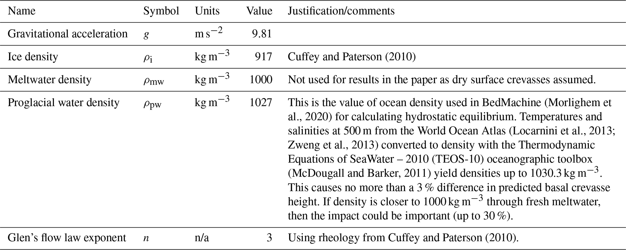
Table A2All variables used with their symbols, units, and comments.
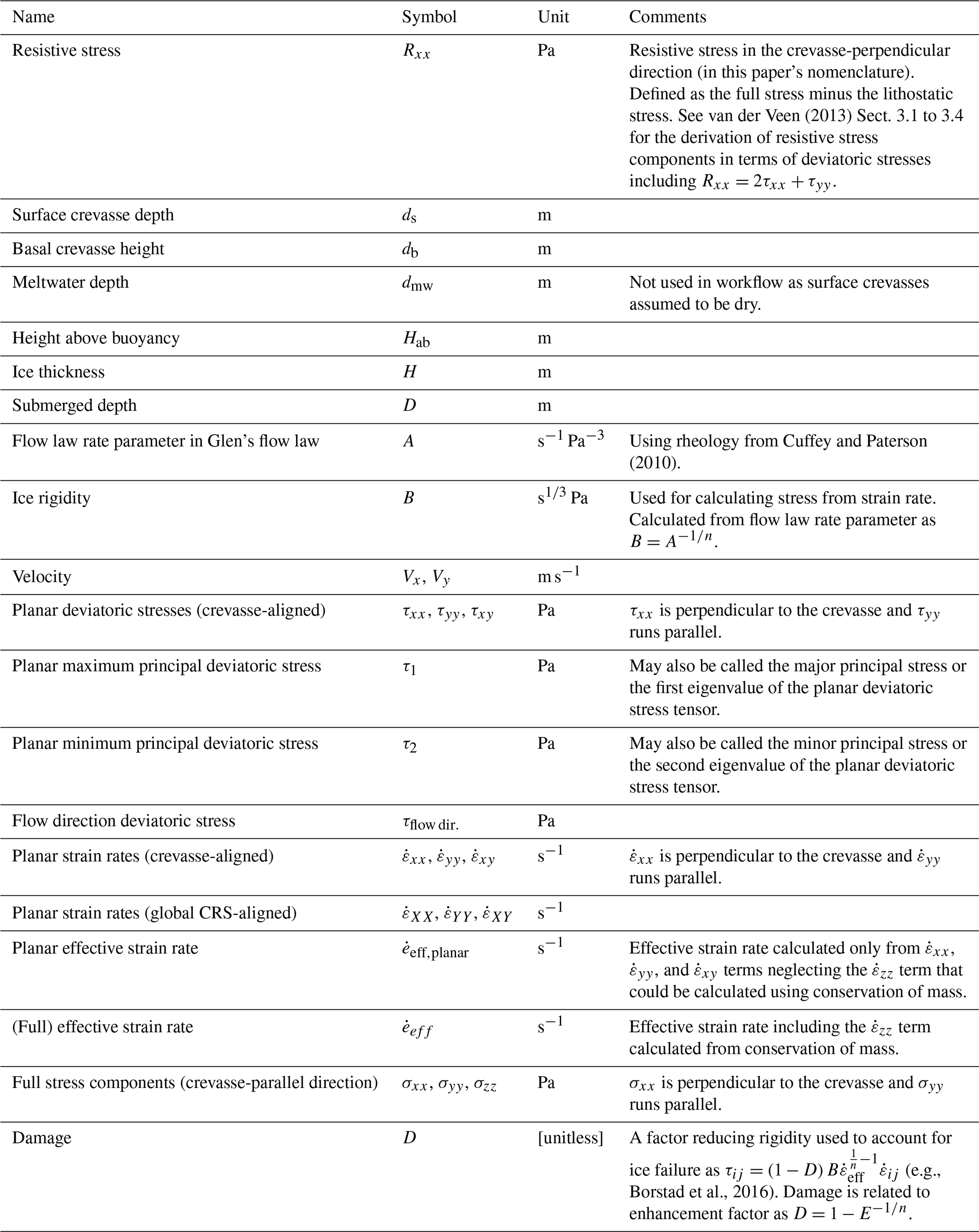
A Python function that calculates resistive stress and then surface crevasse depths and basal crevasse heights with the zero stress approximation is available at https://doi.org/10.5281/zenodo.15420465 (Reynolds et al., 2025). The repository also includes a Jupyter notebook and downsampled data files to reproduce the minimum to maximum principal strain rate ratio plots (Fig. 4c and d) as well as crevasse penetration (Fig. 5) and crevasse penetration difference between calculation plots (Fig. 6). ISSM is available at https://issm.jpl.nasa.gov/ (last access: 12 October 2025).
The fields used to create any of the figures are available by request. The data used in this work are publicly available. NASA ITS_LIVE annual velocity mosaics can be found at https://doi.org/10.5067/6II6VW8LLWJ7 (Gardner et al., 2022). The MEaSUREs 2014–2017 velocity mosaics (and other multiyear mosaics) are available here: https://doi.org/10.5067/FB851ZIZYX5O (Rignot et al., 2022). The temperature data from Comiso (2000) can be found in the example datasets for ISSM here: https://issm.jpl.nasa.gov/documentation/tutorials/datasets/ (last access: 12 October 2025). The BedMachine product including the REMA surface elevation mosaic can be found here: https://doi.org/10.5067/FPSU0V1MWUB6 (Morlighem, 2022).
The supplement related to this article is available online at https://doi.org/10.5194/tc-19-5045-2025-supplement.
BR did conceptualization, methodology, software, visualization, and original draft writing. SN did conceptualization, manuscript review and editing, funding acquisition, and supervision. KP did conceptualization and manuscript review and editing.
At least one of the (co-)authors is a member of the editorial board of The Cryosphere. The peer-review process was guided by an independent editor, and the authors also have no other competing interests to declare.
Publisher's note: Copernicus Publications remains neutral with regard to jurisdictional claims made in the text, published maps, institutional affiliations, or any other geographical representation in this paper. While Copernicus Publications makes every effort to include appropriate place names, the final responsibility lies with the authors. Views expressed in the text are those of the authors and do not necessarily reflect the views of the publisher.
DEMs were provided by the Byrd Polar and Climate Research Center and the Polar Geospatial Center under NSF-OPP awards 1043681, 1542736, 1543501, 1559691, 1810976, and 2129685. The scientific color maps used in all plan-view plots come from Crameri et al. (2020). Benjamin Reynolds and Sophie Nowicki were supported by the NASA Modeling, Analysis, and Prediction Program, the NASA Sea Level Change Team and the National Science Foundation. We also thank the editor, Ruth Mottram, as well Ravindra Duddu and an anonymous reviewer for their suggestions that have improved this paper.
This research has been supported by the National Science Foundation, Directorate for Geosciences (grant no. 2004826), the National Aeronautics Space Administration Sea Level Change Team (grant no. 80NSSC24K1545), and Modeling Analysis and Prediction Program (grant no. 80NSSC25K7094).
This paper was edited by Ruth Mottram and reviewed by Ravindra Duddu and one anonymous referee.
Albrecht, T. and Levermann, A.: Fracture-induced softening for large-scale ice dynamics, The Cryosphere, 8, 587–605, https://doi.org/10.5194/tc-8-587-2014, 2014.
Alley, K. E., Scambos, T. A., Alley, R. B., and Holschuh, N.: Troughs developed in ice-stream shear margins precondition ice shelves for ocean-driven breakup, Sci. Adv., 5, eaax2215, https://doi.org/10.1126/sciadv.aax2215, 2019.
Amaral, T., Bartholomaus, T. C., and Enderlin, E. M.: Evaluation of Iceberg Calving Models Against Observations From Greenland Outlet Glaciers, J. Geophys. Res.-Earth Surf., 125, e2019JF005444, https://doi.org/10.1029/2019JF005444, 2020.
Anderson, T. L.: Fracture mechanics: fundamentals and applications, 3rd edn., Taylor & Francis, Boca Raton, FL, ISBN 9780429125676, https://doi.org/10.1201/9781420058215, 2005.
Bassis, J. N. and Walker, C. C.: Upper and lower limits on the stability of calving glaciers from the yield strength envelope of ice, P. Roy. Soc. A, 468, 913–931, https://doi.org/10.1098/rspa.2011.0422, 2011.
Baurley, N. R., Robson, B. A., and Hart, J. K.: Long-term impact of the proglacial lake Jökulsárlón on the flow velocity and stability of Breiðamerkurjökull glacier, Iceland, Earth Surface Processes and Landforms, 45, 2647–2663, https://doi.org/10.1002/esp.4920, 2020.
Benn, D. I., Hulton, N. R. J., and Mottram, R. H.: `Calving laws', `sliding laws' and the stability of tidewater glaciers, Ann. Glaciol., 46, 123–130, https://doi.org/10.3189/172756407782871161, 2007.
Benn, D. I., Todd, J., Luckman, A., Bevan, S., Chudley, T. R., Astroem, J., Zwinger, T., Cook, S., and Christoffersen, P.: Controls on calving at a large Greenland tidewater glacier: stress regime, self-organised criticality and the crevasse-depth calving law, J. Glaciol., https://doi.org/10.1017/jog.2023.81, 2023.
Berg, B. and Bassis, J.: Crevasse advection increases glacier calving, J. Glaciol., 68, 977–986, https://doi.org/10.1017/jog.2022.10, 2022.
Björnsson, H., Pálsson, F., and Guðmundsson, S.: Jökulsárlón at Breiðamerkursandur, Vatnajökull, Iceland: 20th century changes and future outlook, Jökull, 50, 1–18, https://doi.org/10.33799/jokull2001.50.001, 2001.
Bondzio, J. H., Morlighem, M., Seroussi, H., Kleiner, T., Rückamp, M., Mouginot, J., Moon, T., Larour, E. Y., and Humbert, A.: The mechanisms behind Jakobshavn Isbræ's acceleration and mass loss: A 3-D thermomechanical model study, Geophys. Res. Lett., 44, 6252–6260, https://doi.org/10.1002/2017GL073309, 2017.
Buck, W. R.: The role of fresh water in driving ice shelf crevassing, rifting and calving, Earth and Planetary Science Letters, 624, 118444, https://doi.org/10.1016/j.epsl.2023.118444, 2023.
Borstad, C., Khazendar, A., Scheuchl, B., Morlighem, M., Larour, E., and Rignot, E.: A constitutive framework for predicting weakening and reduced buttressing of ice shelves based on observations of the progressive deterioration of the remnant Larsen B Ice Shelf, Geophys. Res. Lett., 43, 2027–2035, https://doi.org/10.1002/2015GL067365, 2016.
Borstad, C. P., Khazendar, A., Larour, E., Morlighem, M., Rignot, E., Schodlok, M. P., and Seroussi, H.: A damage mechanics assessment of the Larsen B ice shelf prior to collapse: Toward a physically-based calving law, Geophys. Res. Lett., 39, https://doi.org/10.1029/2012GL053317, 2012.
Choi, Y., Morlighem, M., Wood, M., and Bondzio, J. H.: Comparison of four calving laws to model Greenland outlet glaciers, The Cryosphere, 12, 3735–3746, https://doi.org/10.5194/tc-12-3735-2018, 2018.
Clayton, T., Duddu, R., Siegert, M., and Martínez-Pañeda, E.: A stress-based poro-damage phase field model for hydrofracturing of creeping glaciers and ice shelves, Engineering Fracture Mechanics, 272, 108693, https://doi.org/10.1016/j.engfracmech.2022.108693, 2022.
Clayton, T., Duddu, R., Hageman, T., and Martínez-Pañeda, E.: The influence of firn layer material properties on surface crevasse propagation in glaciers and ice shelves, The Cryosphere, 18, 5573–5593, https://doi.org/10.5194/tc-18-5573-2024, 2024.
Coffey, N. B., Lai, C.-Y., Wang, Y., Buck, W. R., Surawy-Stepney, T., and Hogg, A. E.: Theoretical stability of ice shelf basal crevasses with a vertical temperature profile, J. Glaciol., 70, e64, https://doi.org/10.1017/jog.2024.52, 2024.
Colgan, W., Rajaram, H., Abdalati, W., McCutchan, C., Mottram, R., Moussavi, M. S., and Grigsby, S.: Glacier crevasses; observations, models, and mass balance implications, Rev. Geophys., 54, 119–161, https://doi.org/10.1002/2015RG000504, 2016.
Comiso, J. C.: Variability and Trends in Antarctic Surface Temperatures from In Situ and Satellite Infrared Measurements, J. Climate, 13, 1674–1696, https://doi.org/10.1175/1520-0442(2000)013<1674:VATIAS>2.0.CO;2, 2000.
Crameri, F., Shephard, G. E., and Heron, P. J.: The misuse of colour in science communication, Nat. Commun., 11, 5444, https://doi.org/10.1038/s41467-020-19160-7, 2020.
Cuffey, K. M. and Paterson, W. S. B.: The Physics of Glaciers, 4th edn., Elsevier, Burlington, MA, ISBN 9780123694614, 2010.
Dahl-Jensen, D.: Steady thermomechanical flow along two-dimensional flow lines in large grounded ice sheets, J. Geophys. Res.-Sol. Ea., 94, 10355–10362, https://doi.org/10.1029/JB094iB08p10355, 1989.
Duddu, R., Jiménez, S., and Bassis, J.: A non-local continuum poro-damage mechanics model for hydrofracturing of surface crevasses in grounded glaciers, J. Glaciol., 66, 415–429, https://doi.org/10.1017/jog.2020.16, 2020.
Echelmeyer, K. A., Harrison, W. D., Larsen, C., and Mitchell, J. E.: The role of the margins in the dynamics of an active ice stream, J. Glaciol., 40, 527–538, https://doi.org/10.3189/S0022143000012417, 1994.
Enderlin, E. M. and Bartholomaus, T. C.: Sharp contrasts in observed and modeled crevasse patterns at Greenland's marine terminating glaciers, The Cryosphere, 14, 4121–4133, https://doi.org/10.5194/tc-14-4121-2020, 2020.
Fürst, J. J., Durand, G., Gillet-Chaulet, F., Tavard, L., Rankl, M., Braun, M., and Gagliardini, O.: The safety band of Antarctic ice shelves, Nat. Clim. Change, 6, 479–482, https://doi.org/10.1038/nclimate2912, 2016.
Gao, Y., Ghosh, G., Jiménez, S., and Duddu, R.: A Finite-Element-Based Cohesive Zone Model of Water-Filled Surface Crevasse Propagation in Floating Ice Tongues, Comput. Sci. Eng., 25, 8–16, https://doi.org/10.1109/MCSE.2023.3315661, 2023.
Gardner, A. S., Moholdt, G., Scambos, T., Fahnstock, M., Ligtenberg, S., van den Broeke, M., and Nilsson, J.: Increased West Antarctic and unchanged East Antarctic ice discharge over the last 7 years, The Cryosphere, 12, 521–547, https://doi.org/10.5194/tc-12-521-2018, 2018.
Gardner, A. S., Fahnestock, M., and Scambos, T.: MEaSUREs ITS_LIVE Regional Glacier and Ice Sheet Surface Velocities. (NSIDC-0776, Version 1), Boulder, Colorado USA, NASA National Snow and Ice Data Center Distributed Active Archive Center [data set], https://doi.org/10.5067/6II6VW8LLWJ7, 2022.
Glen, J. W.: Experiments on the Deformation of Ice, J. Glaciol., 2, 111–114, https://doi.org/10.3189/S0022143000034067, 1952.
Goldsby, D. L. and Kohlstedt, D. L.: Superplastic deformation of ice: Experimental observations, J. Geophys. Res.-Sol. Ea., 106, 11017–11030, https://doi.org/10.1029/2000JB900336, 2001.
Gudmundsson, G. H.: Ice-shelf buttressing and the stability of marine ice sheets, The Cryosphere, 7, 647–655, https://doi.org/10.5194/tc-7-647-2013, 2013.
Guðmundsson, S., Björnsson, H., and Pálsson, F.: Changes of Breiðamerkurjökull glacier, SE-Iceland, from its late nineteenth century maximum to the present, Geografiska Annaler: Series A, Physical Geography, 99, 338–352, https://doi.org/10.1080/04353676.2017.1355216, 2017.
Howat, I. M., Porter, C., Smith, B. E., Noh, M.-J., and Morin, P.: The Reference Elevation Model of Antarctica, The Cryosphere, 13, 665–674, https://doi.org/10.5194/tc-13-665-2019, 2019.
Hulbe, C. L., Klinger, M., Masterson, M., Catania, G., Cruikshank, K., and Bugni, A.: Tidal bending and strand cracks at the Kamb Ice Stream grounding line, West Antarctica, J. Glaciol., 62, 816–824, https://doi.org/10.1017/jog.2016.74, 2016.
Humbert, A.: The temperature regime of Fimbulisen, Antarctica, Ann. Glaciol., 51, 56–64, https://doi.org/10.3189/172756410791392673, 2010.
Huth, A., Duddu, R., and Smith, B.: A Generalized Interpolation Material Point Method for Shallow Ice Shelves. 2: Anisotropic Nonlocal Damage Mechanics and Rift Propagation, J. Adv. Model. Earth Sy., 13, e2020MS002292, https://doi.org/10.1029/2020MS002292, 2021.
Jezek, K. C.: A modified theory of bottom crevasses used as a means for measuring the buttressing effect of ice shelves on inland ice sheets, J. Geophys. Res.-Sol. Ea., 89, 1925–1931, https://doi.org/10.1029/JB089iB03p01925, 1984.
Jiménez, S. and Duddu, R.: On the evaluation of the stress intensity factor in calving models using linear elastic fracture mechanics, J. Glaciol., 64, 759–770, https://doi.org/10.1017/jog.2018.64, 2018.
Khazendar, A., Borstad, C. P., Scheuchl, B., Rignot, E., and Seroussi, H.: The evolving instability of the remnant Larsen B Ice Shelf and its tributary glaciers, Earth Planet. Sc. Lett., 419, 199–210, https://doi.org/10.1016/j.epsl.2015.03.014, 2015.
Lai, C.-Y., Kingslake, J., Wearing, M. G., Chen, P.-H. C., Gentine, P., Li, H., Spergel, J. J., and van Wessem, J. M.: Vulnerability of Antarctica's ice shelves to meltwater-driven fracture, Nature, 584, 574, https://doi.org/10.1038/s41586-020-2627-8, 2020.
Larour, E., Seroussi, H., Morlighem, M., and Rignot, E.: Continental scale, high order, high spatial resolution, ice sheet modeling using the Ice Sheet System Model (ISSM), J. Geophys. Res.-Earth Surf., 117, https://doi.org/10.1029/2011JF002140, 2012.
Lhermitte, S., Sun, S., Shuman, C., Wouters, B., Pattyn, F., Wuite, J., Berthier, E., and Nagler, T.: Damage accelerates ice shelf instability and mass loss in Amundsen Sea Embayment, P. Natl. Acad. Sci. USA, 117, 24735–24741, https://doi.org/10.1073/pnas.1912890117, 2020.
Lipovsky, B. P.: Ice shelf rift propagation: stability, three-dimensional effects, and the role of marginal weakening, The Cryosphere, 14, 1673–1683, https://doi.org/10.5194/tc-14-1673-2020, 2020.
Locarnini, R. A., Mishonov, A. V., Antonov, J. I., Boyer, T. P., Garcia, H. E., Baranova, O. K., Zweng, M. M., Paver, C. R., Reagan, J. R., Johnson, D. R., Hamilton, M., and Seidov, D.: World Ocean Atlas 2013, Volume 1: Temperature. S. Levitus, Ed.; A. Mishonov, Technical Ed.; NOAA Atlas NESDIS 73, 40 pp., https://doi.org/10.7289/V55X26VD, https://doi.org/10.7289/V5F769GT, 2013.
Luckman, A., Jansen, D., Kulessa, B., King, E. C., Sammonds, P., and Benn, D. I.: Basal crevasses in Larsen C Ice Shelf and implications for their global abundance, The Cryosphere, 6, 113–123, https://doi.org/10.5194/tc-6-113-2012, 2012.
Lüthi, M., Funk, M., Iken, A., Gogineni, S., and Truffer, M.: Mechanisms of fast flow in Jakobshavn Isbræ, West Greenland: Part III. Measurements of ice deformation, temperature and cross-borehole conductivity in boreholes to the bedrock, J. Glaciol., 48, 369–385, https://doi.org/10.3189/172756502781831322, 2002.
MacAyeal, D. R.: Large-scale ice flow over a viscous basal sediment: Theory and application to ice stream B, Antarctica, J. Geophys. Res.-Sol. Ea., 94, 4071–4087, https://doi.org/10.1029/JB094iB04p04071, 1989.
Maier, N., Humphrey, N., Harper, J., and Meierbachtol, T.: Sliding dominates slow-flowing margin regions, Greenland Ice Sheet, Sci. Adv., 5, eaaw5406, https://doi.org/10.1126/sciadv.aaw5406, 2019.
McDougall, T. and Barker, P. M.: Getting started with TEOS-10 and the Gibbs Seawater (GSW) Oceanographic Toolbox, SCOR/IAPSO WG, 127, 1–28, 2011.
McGrath, D., Steffen, K., Rajaram, H., Scambos, T. A., Abdalati, W., and Rignot, E.: Basal crevasses on the Larsen C Ice Shelf, Antarctica; implications for meltwater ponding and hydrofracture, Geophys. Res. Lett., 39, https://doi.org/10.1029/2012GL052413, 2012.
Meng, Y., Culberg, R., and Lai, C.-Y.: Vulnerability of firn to hydrofracture: poromechanics modeling, J. Glaciol., 70, e45, https://doi.org/10.1017/jog.2024.47, 2024.
Millstein, J. D., Minchew, B. M., and Pegler, S. S.: Ice viscosity is more sensitive to stress than commonly assumed, Commun. Earth Environ., 3, 1–7, https://doi.org/10.1038/s43247-022-00385-x, 2022.
Mobasher, M. E., Duddu, R., and Waisman, H.: Computational Modeling of Ice Mechanics: A Review of Challenges and Approaches in Engineering and Glaciology, in: Reference Module in Materials Science and Materials Engineering, Elsevier, https://doi.org/10.1016/B978-0-323-90646-3.00025-3, 2024.
Morlighem, M.: MEaSUREs BedMachine Antarctica (NSIDC-0756, Version 3), Boulder, Colorado USA, NASA National Snow and Ice Data Center Distributed Active Archive Center [data set], https://doi.org/10.5067/FPSU0V1MWUB6, 2022.
Morlighem, M., Rignot, E., Binder, T., Blankenship, D., Drews, R., Eagles, G., Eisen, O., Ferraccioli, F., Forsberg, R., Fretwell, P., Goel, V., Greenbaum, J. S., Gudmundsson, H., Guo, J., Helm, V., Hofstede, C., Howat, I., Humbert, A., Jokat, W., Karlsson, N. B., Lee, W. S., Matsuoka, K., Millan, R., Mouginot, J., Paden, J., Pattyn, F., Roberts, J., Rosier, S., Ruppel, A., Seroussi, H., Smith, E. C., Steinhage, D., Sun, B., Broeke, M. R. van den, Ommen, T. D. van, Wessem, M. van, and Young, D. A.: Deep glacial troughs and stabilizing ridges unveiled beneath the margins of the Antarctic ice sheet, Nat. Geosci., 13, 132–137, https://doi.org/10.1038/s41561-019-0510-8, 2020.
Mottram, R. H. and Benn, D. I.: Testing crevasse-depth models: a field study at Breiðamerkurjökull, Iceland, J. Glaciol., 55, 746–752, https://doi.org/10.3189/002214309789470905, 2009.
Nick, F., Veen, C. J., Vieli, A., and Benn, D.: A physically based calving model applied to marine outlet glaciers and implications for the glacier dynamics, J. Glaciol., 56, 781–794, https://doi.org/10.3189/002214310794457344, 2010.
Nye, J. F.: The Flow Law of Ice from Measurements in Glacier Tunnels, Laboratory Experiments and the Jungfraufirn Borehole Experiment, P. Roy. Soc. Lond. A, 219, 477–489, 1953.
Nye, J. F.: Comments on Dr. Loewe's Letter and Notes on Crevasses, J. Glaciol., 2, 512–514, https://doi.org/10.3189/S0022143000032652, 1955.
Pollard, D., DeConto, R. M., and Alley, R. B.: Potential Antarctic Ice Sheet retreat driven by hydrofracturing and ice cliff failure, Earth Planet. Sc. Lett., 412, 112–121, https://doi.org/10.1016/j.epsl.2014.12.035, 2015.
Reynolds, B., Nowicki, S., and Poinar, K.: Resistive stress / Nye crevasse formulation demo code for “Comprehensive Assessment of Stress Calculations for Crevasse Depths and Testing with Crevasse Penetration as Damage”, Zenodo [code], https://doi.org/10.5281/zenodo.15420465, 2025.
Rignot, E., Casassa, G., Gogineni, P., Krabill, W., Rivera, A., and Thomas, R.: Accelerated ice discharge from the Antarctic Peninsula following the collapse of Larsen B ice shelf, Geophys. Res. Lett., 31, https://doi.org/10.1029/2004GL020697, 2004.
Rignot, E., Scheuchl, B., Mouginot, J., and Jeong, S.: MEaSUREs Multi-year Reference Velocity Maps of the Antarctic Ice Sheet (NSIDC-0761, Version 1), Boulder, Colorado USA, NASA National Snow and Ice Data Center Distributed Active Archive Center [data set], https://doi.org/10.5067/FB851ZIZYX5O, 2022.
Rist, M. A., Sammonds, P. R., Murrell, S. a. F., Meredith, P. G., Oerter, H., and Doake, C. S. M.: Experimental fracture and mechanical properties of Antarctic ice: preliminary results, Ann. Glaciol., 23, 284–292, https://doi.org/10.3189/S0260305500013550, 1996.
Rott, H., Müller, F., Nagler, T., and Floricioiu, D.: The imbalance of glaciers after disintegration of Larsen-B ice shelf, Antarctic Peninsula, The Cryosphere, 5, 125–134, https://doi.org/10.5194/tc-5-125-2011, 2011.
Schoof, C.: Ice sheet grounding line dynamics: Steady states, stability, and hysteresis, J. Geophys. Res.-Earth Surf., 112, https://doi.org/10.1029/2006JF000664, 2007.
Scott, J. B. T., Smith, A. M., Bingham, R. G., and Vaughan, D. G.: Crevasses triggered on Pine Island Glacier, West Antarctica, by drilling through an exceptional melt layer, Ann. Glaciol., 51, 65–70, https://doi.org/10.3189/172756410791392763, 2010.
Shabana, A. A.: Computational continuum mechanics, 3rd edn., Wiley, Hoboken, New Jersey, ISBN 9781119293248, https://doi.org/10.1002/9781119293248, 2018.
Smith, R. A.: The Application of Fracture Mechanics to the Problem of Crevasse Penetration, J. Glaciol., 17, 223–228, https://doi.org/10.3189/S0022143000013563, 1976.
Sun, S., Cornford, S. L., Moore, J. C., Gladstone, R., and Zhao, L.: Ice shelf fracture parameterization in an ice sheet model, The Cryosphere, 11, 2543–2554, https://doi.org/10.5194/tc-11-2543-2017, 2017.
Surawy-Stepney, T., Hogg, A. E., Cornford, S. L., and Davison, B. J.: Episodic dynamic change linked to damage on the Thwaites Glacier Ice Tongue, Nat. Geosci., 16, 37–43, https://doi.org/10.1038/s41561-022-01097-9, 2023.
Todd, J., Christoffersen, P., Zwinger, T., Råback, P., Chauché, N., Benn, D., Luckman, A., Ryan, J., Toberg, N., Slater, D., and Hubbard, A.: A Full-Stokes 3-D Calving Model Applied to a Large Greenlandic Glacier, J. Geophys. Res.-Earth Surf., 123, 410–432, https://doi.org/10.1002/2017JF004349, 2018.
van der Veen, C. J.: Fracture mechanics approach to penetration of surface crevasses on glaciers, Cold Reg. Sci. Technol., 27, 31–47, https://doi.org/10.1016/S0165-232X(97)00022-0, 1998a.
van der Veen, C. J.: Fracture mechanics approach to penetration of bottom crevasses on glaciers, Cold Reg. Sci. Technol., 27, 213–223, https://doi.org/10.1016/S0165-232X(98)00006-8, 1998b.
van der Veen, C. J.: Crevasses on glaciers 1, Polar Geography, 23, 213–245, https://doi.org/10.1080/10889379909377677, 1999.
van der Veen, C. J., Plummer, J. C., and Stearns, L. A.: Controls on the recent speed-up of Jakobshavn Isbræ, West Greenland, J. Glaciol., 57, 770–782, https://doi.org/10.3189/002214311797409776, 2011.
van der Veen, C. J.: Fundamentals of glacier dynamics, 2nd edn., CRC Press, Boca Raton, FL, https://doi.org/10.1201/b14059, 2013.
van der Veen, C. J. and Whillans, I. M.: Force Budget: I. Theory and Numerical Methods, J. Glaciol., 35, 53–60, https://doi.org/10.3189/002214389793701581, 1989.
van de Wal, R. S. W., Nicholls, R. J., Behar, D., McInnes, K., Stammer, D., Lowe, J. A., Church, J. A., DeConto, R., Fettweis, X., Goelzer, H., Haasnoot, M., Haigh, I. D., Hinkel, J., Horton, B. P., James, T. S., Jenkins, A., LeCozannet, G., Levermann, A., Lipscomb, W. H., Marzeion, B., Pattyn, F., Payne, A. J., Pfeffer, W. T., Price, S. F., Seroussi, H., Sun, S., Veatch, W., and White, K.: A High-End Estimate of Sea Level Rise for Practitioners, Earth's Future, 10, e2022EF002751, https://doi.org/10.1029/2022EF002751, 2022.
Van Wyk de Vries, M., Lea, J. M., and Ashmore, D. W.: Crevasse density, orientation and temporal variability at Narsap Sermia, Greenland, J. Glaciol., 69, 1125–1137, https://doi.org/10.1017/jog.2023.3, 2023.
Wang, Y., Zhao, C., Gladstone, R., Galton-Fenzi, B., and Warner, R.: Thermal structure of the Amery Ice Shelf from borehole observations and simulations, The Cryosphere, 16, 1221–1245, https://doi.org/10.5194/tc-16-1221-2022, 2022.
Weertman, J.: Can a water-filled crevasse reach the bottom surface of a glacier?, International Association of Scientific Hydrology–Association Internationale d'Hydrologie Scientifique (International Union of Geodesy and Geophysics–Union de Geodesie et de Geophysique Internationale), Publication, Louvain, 95, 139–145, 1973.
Weertman, J.: Bottom Crevasses, J. Glaciol., 25, 185–188, https://doi.org/10.3189/S0022143000010418, 1980.
Wilner, J. A., Morlighem, M., and Cheng, G.: Evaluation of four calving laws for Antarctic ice shelves, The Cryosphere, 17, 4889–4901, https://doi.org/10.5194/tc-17-4889-2023, 2023.
Zweng, M. M., Reagan, J. R., Antonov, J. I., Locarnini, R. A., Mishonov, A. V., Boyer, T. P., Garcia, H. E., Baranova, O. K., Johnson, D. R., Seidov, D., and Biddle, M. M.: World Ocean Atlas 2013, Volume 2: Salinity, S. Levitus, Ed.; A. Mishonov, Technical Ed.; NOAA Atlas NESDIS 74, 39 pp., https://doi.org/10.7289/V5251G4D, 2013