Sea ice in the Baltic Sea during 1993/94–2020/21 ice seasons from satellite observations and model reanalysis

This study investigates the sea ice characteristics of the Baltic Sea using Copernicus satellite and model reanalysis data products from 1993 onward. Our primary focus is on assessing the performance of the latest Copernicus model reanalysis product in estimating the ice season evolution compared to the satellite dataset. The model estimates an earlier start to the ice season; it generally matches satellite data regarding the season's end. In addition, the model ice thickness is compared with the ice chart-based data. Across the Baltic Sea, declining trends for sea ice are observed. The sea ice characteristics during the recent period (2007/08–2020/21) show decreased sea ice fraction and thickness compared to the preceding period (1993/94–2006/07) of the study. The decrease in sea ice thickness is greater than 50 % in some areas during the spring season. The trend analysis in the study reveals a uniform pattern toward shorter ice seasons (the most prominent being in Bothnian Bay with a range of approximately 1–3 d yr⁻¹ of decline in ice season), reduced sea ice extent (SIE) and reduced mean ice thickness (reaching up to −0.7 cm yr⁻¹).

1 Introduction

The Baltic Sea is a semi-enclosed sea located in Northern Europe, recognized as a shelf sea and a marginal sea of the Atlantic. It stands as one of the most extensive brackish water bodies globally (Voipio, 1981). The sea undergoes seasonal fluctuations in ice coverage (Leppäranta and Myrberg, 2009). It is a crucial economic zone, hosting one of the densest shipping networks in the world and significant economic interests (International Maritime Organization (IMO)). Operations in this region are greatly influenced by the presence of sea ice. Hence, the precise modeling and forecasting of the sea ice season in the Baltic Sea hold significant importance for ensuring secure navigation, particularly for maritime transport, fishing fleets, and various commercial ventures like the construction of offshore wind farms. Accurate spatio–temporal observations and predictions also offer important insights into climate patterns, fluctuations in ice coverage, and the broader shifts in the region's environment. During severe winters, Finland and Estonia stand out as the only countries worldwide where all harbors undergo complete freezing (Jevrejeva and Leppäranta, 2002), an important occurrence that amplifies the priority placed on sea ice studies in the region.

The state of sea ice is important for many stakeholders (Wagner et al., 2020). Monitoring the extent and thickness of the Baltic ice cover, as well as the duration of the ice season, has been crucial for navigation and travel for centuries. Severe sea ice conditions have the potential to substantially disrupt the flow of busy Baltic maritime traffic (Löptien and Axell, 2014). The duration of ice cover in the Baltic Sea significantly impacts spring biota activity, altering the timing of spring blooms and the composition of phytoplankton species (Klais et al., 2017a, b; Pärn et al., 2021), thereby affecting nutrient cycles and ecosystem dynamics (Klais et al., 2013), which may have significant implications for fisheries industries. To address these needs of various user groups, Digital Twins and their applications for European waters (including the Baltic Sea) are being developed under the Destination Earth and EDITO (European Digital Twin of the Ocean) initiatives. Thus, accurate information and analysis of sea ice conditions/processes in the Baltic Sea, provided in the current study over different spatio-temporal scales (from operational monitoring to climate analysis), are also relevant for the development of Digital Twins and related impact models (Åström et al., 2024). The improved sea ice information that can be ingested into the Digital Twins applications and tools enables what-if scenario analyses and improves the planning of offshore activities.

The exploration of sea ice dynamics and climatology has been a focal point in numerous studies (Leppäranta, 1981; Haapala and Leppäranta, 1997; Granskog et al., 2006; Siitam et al., 2017; Raudsepp et al., 2020). Haapala and Leppäranta (1996) studied the climatology of the Baltic Sea ice season, using three particular winters (normal, severe, and mild winters) and concluded that a moderate resolution ice-ocean model could reproduce the main characteristics of the ice season. The typical duration of the ice season spans up to seven months (Vihma and Haapala, 2009), peaking in late February and early March (BACC Author Team, 2008), when on average the ice covered area is 45 % of the total area of the Baltic Sea (Leppäranta and Myrberg, 2009). While March usually marks the onset of melting, observations in the northernmost Bothnian Bay have recorded ice persisting until June (Leppäranta and Myrberg, 2009). The duration of the ice season varies from some 20 to 30 d in the northern Baltic Proper to more than 6 months in the northern Bothnian Bay (Jevrejeva et al., 2004). In the Gulf of Riga sub-basin, the length of the ice season observed from remote sensing data is in the range of 3–4.5 months (Siitam et al., 2017). Due to thicker ice and colder climate, ice persists longer in the Bothnian Bay compared to other sub-basins in the Baltic Sea (Pemberton et al., 2017). However, the sub-basins Bothnian Bay, Bothnian Sea, Gulf of Finland, and the Gulf of Riga show a coherent pattern of interannual variability in the timing and length of the ice season (Raudsepp et al., 2020). Long-term time series data suggest a shift towards milder winters: for example, a decreasing trend of 14 to 44 d in ice season length was observed during the 20th century (Jevrejeva et al., 2004). A shift in the ice season regime from 2008 was reported, which resulted in reduced ice cover and season length (Pärn et al., 2022). Recent years have shown a continued decrease in the duration of the ice season and a rapid warming during spring across all sub-basins (Pärn et al., 2022).

Remote sensing techniques have evolved to enhance the efficacy of ice information services (Karvonen, 2013, 2017, 2021; Leppäranta and Lewis, 2007; Mäkynen and Hallikainen, 2005). The studies regarding sea ice in the Baltic Sea have utilized different datasets. In the 2004 study, Jevrejeva et al. (2004) used the station data, whereas in a recent study by Pärn et al. (2022), datasets from Copernicus Marine Environment Monitoring Service (von Schuckmann et al., 2018) and ERA5 (Hersbach et al., 2020) of European Centre for Medium–range Weather forecast (ECMWF) were used. Nevertheless, remote sensing techniques offer restricted insights into sea ice thickness. Hence model reanalysis data have been utilized for the sea ice thickness analysis.

The Copernicus Marine Service (or Copernicus Marine Environment Monitoring Service) is the marine component of the Copernicus Programme of the European Union. It provides free, regular, and systematic authoritative information on the state of the Blue (physical), White (sea ice), and Green (biogeochemical) ocean, on a global and regional scale. The analysis has utilized the latest model reanalysis Baltic physics product and satellite based products (all described in the upcoming section) from the service for the Baltic Sea. With the recent updates in the regional reanalysis of the Baltic Sea, the new model product has improved spatial resolution and updated sea ice model (Kärnä et al., 2021), which provides an improved description of the ice state over previous model products (Panteleit et al., 2019).

Objectives

An integral objective of this study was to examine the spatial and temporal disparities between sea ice characteristics from the new release of Copernicus Marine Service Baltic Sea Physics reanalysis product (BALTICSEA_MULTIYEAR_PHY_003_011) to the satellite and ice chart–based datasets. This comparison aims to assess the accuracy of the model–simulated data in reproducing the observed characteristics of the Baltic Sea ice. The specific objectives are (a) finding the sea ice fraction threshold (TH_SIF) to bias correct (minimize bias) the model reanalysis dataset for sea ice extent (SIE) and comparing ice thickness statistics between the model and SAR & ice charts–based datasets; (b) comparing Baltic Sea Physics reanalysis product's sea ice season evolution characteristics with satellite dataset; (c) analyzing the characteristics and changes of ice extent and thickness during 1993/94–2020/21; (d) providing trend analysis of the sea ice season parameters and sea ice thickness.

2 Datasets

The study utilized the Copernicus Marine Sea Surface Temperature (SST) dataset from the reprocessed L4 product which contains Sea Ice Fraction (SIF) data. The Copernicus Marine SST reprocessed L4 product, known as SST_BAL_SST_L4_REP_OBSERVATIONS_010_016 (Høyer and Karagali, 2016) has been developed at the Danish Meteorological Institute (DMI) and offers comprehensive, gap–free maps of sea surface temperature (SST) for the Baltic Sea region. The L4 product is made at a high resolution of 2.4×1.44 km (0.02° × 0.02°) using satellite data from ESA's SST CCI and Copernicus C3S projects, incorporating an array of different sensors on satellites like NOAA AVHRRs Metop, ATSR1, ATSR2, AATSR, and SLSTR. It also combines this data with in situ measurements from the HadIOD dataset and high-resolution sea ice information from Swedish Meteorological and Hydrological Institute (SMHI) and Finnish Meteorological Institute (FMI). The sea ice fraction data in the product is taken from the sea ice charts from the national ice services at FMI and SMHI, based on manual interpretation by the operator. The product data is available daily from 1 January 1982 to 31 December 2023. The derived L4 sea surface temperature (SST) used in the product has been compared with different sources of in situ observations by Nielsen-Englyst et al. (2023). Hereafter in the study, this dataset is referred to as the satellite dataset.

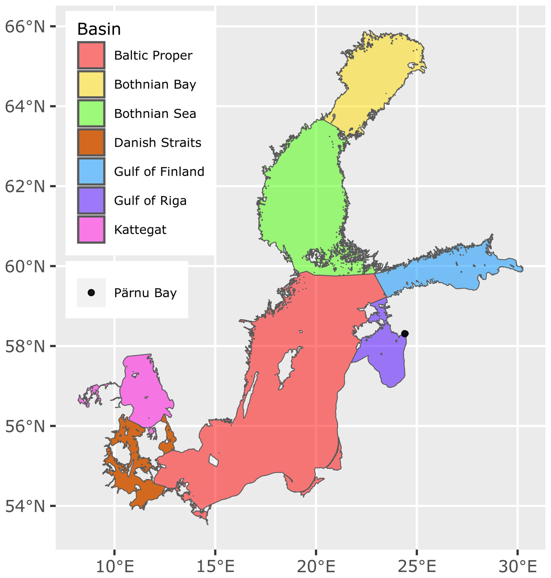
Figure 1 Spatial Distribution of Baltic Sea sub-basins. Figure illustrates the distinct geographical boundaries of Baltic Sea sub-basins–Bothnian Bay (BB), Bothnian Sea (BS), Gulf of Finland (GoF), Gulf of Riga (GoR), Baltic Proper (BP), Danish Straits (DS) and Kattegat–represented in unique colors for differentiation. The sub-basins are based on the PLC–6 project, and are obtained from the Helsinki Commission (HELCOM, 2018).

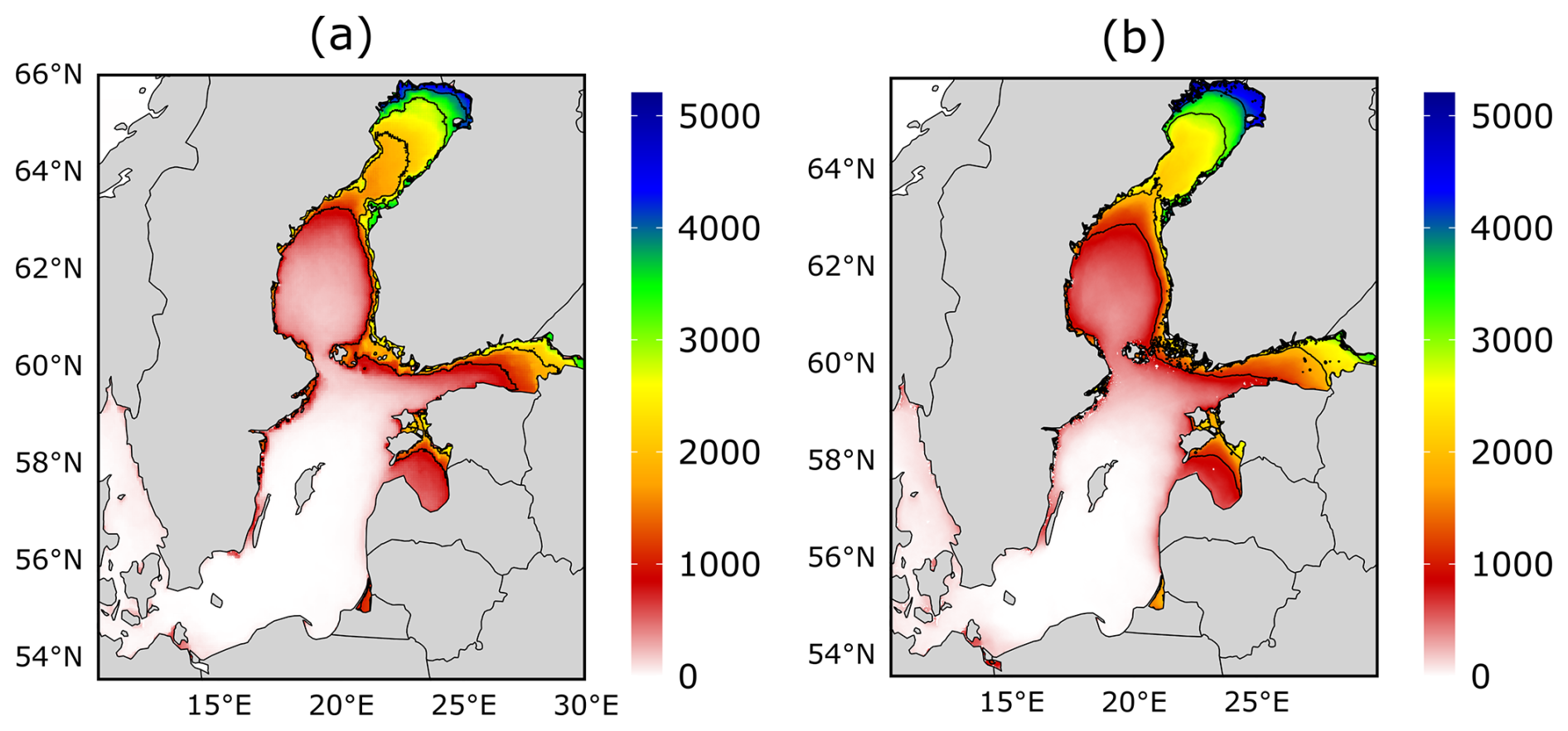
Figure 2 The sample size of the datasets used in the calculations, panels (a) and (b) illustrate the aggregated days factored into the calculations at individual grid point (solid thin black contour lines are at value of 1000, 2000, 3000, and 4000 d) from satellite and model data respectively.

The latest reprocessing product (released in March 2023), Copernicus Marine Baltic Sea Physics Reanalysis (BALTICSEA_MULTIYEAR_PHY_003_011) have been used in the study. The study utilizes Sea Ice Fraction (SIF) and Sea Ice Thickness (SIT) parameters from this new dataset. The product is based on simulations using the 3D ocean–ice model NEMO (Nucleus for European Modelling of the Ocean) regional Nemo–Nordic 2.0 configuration (Kärnä et al., 2021). It offers a comprehensive reanalysis of physical conditions in the Baltic Sea available daily from 1 January 1993 to 31 December 2021, providing a 2×2 km (0.0277° × 0.0166°) grid resolution. The physical system assimilates satellite sea surface temperature, in situ temperature and salinity profiles. The system is forced by ECMWF ERA5 meteorology (Hersbach et al., 2020). The fully coupled sea ice model SI3 addresses various aspects of sea ice dynamics, including thermodynamics, advection, rheology, and the processes of ridging and rafting. The land fast ice parametrization utilized in this model follows the approach outlined by Lemieux et al. (2016). The model comprises five ice categories and one snow category, with specified thickness bounds set at 0.45, 1.13, 2.14, and 3.67 m. In this work, the standard settings within the sea ice model, without ice assimilation, originally developed for the global ocean for defining the ice thickness categories, are used. Subsequently in the study, this dataset is referred to as the model dataset.

The level ice thickness data from the Copernicus Marine Baltic Sea–Sea Ice Concentration and Thickness Charts product dataset with product id SEAICE_BAL_SEAICE_L4_NRT_OBSERVATIONS_011_ 004 (Karvonen et al., 2007) has been used in the study to compare the ice thickness statistics with the model dataset. This dataset has 1×1 km spatial resolution and is available daily from 1 January 2018 to 5 June 2024. The ice parameters in the product are based on SAR image and ice chart produced on a daily basis during the Baltic Sea ice season provided by FMI and SMHI. The product is validated against icebreaker ice thickness data (Berglund and Molinier, 2014) in the Quality Information Document file (CMEMS-SEAICE-QUID-004_011_019, issue 1.1). This is referred to as the SAR & ice charts–based product in the study.

Although ice chart-based sea ice data may have some uncertainties, these datasets have been reliably used in numerous studies to validate other products such as model products (Mäkynen et al., 2020; Karvonen, 2021; Pärn et al., 2021; Leppäranta, 2023) and are available over an extended period. Due to the lack of a better automated tool for interpreting high-resolution sea ice imagery and the limited field observations, ice charts are considered the most accurate datasets for representing the true state of sea ice, and thus other sea ice data sets use them as reference (CMEMS-SI-QUID-011-001to007-009to014, issue 2.10).

The geographical boundaries of the sub-basins used in current study are based on the PLC–6 project, obtained from Helsinki Commision (https://maps.helcom.fi/website/mapservice/?datasetID=1456f8a5-72a2-4327-8894-31287086ebb5, last access: 15 January 2025), shown in Fig. 1. The satellite dataset spans from 1993/94 to 2020/21, the 2012/13 season was excluded (due to the absence of satellite data for the entire season), resulting in a study period covering 27 ice seasons. However, due to the absence of sea ice (absence here refers to sea ice below TH_SIF, explained in the subsequent section) at specific grid points in the Baltic Sea during different years, the data sample size varies across locations. Figure 2 shows this variation, where (a) and (b) represent the sample count of days used in the study. So the calculations of the ice season parameters were based on the data sample size shown in Fig. 2. The procedure employed in the study for calculation of these parameters is given in the subsequent methodology section.

3 Methodology

The analysis of sea ice statistics in the Baltic Sea region relied on satellite and model datasets, which were used for the calculation of the annual ice season parameters for the study period. For the satellite dataset, a sea ice fraction threshold (TH_SIF) of 0.15 was applied, while the model dataset utilized a TH_SIF of 0.20. The reasoning for choosing these thresholds is given in the subsequent section.

Identification of the onset date of sea ice formation at each grid point (i, j) was established when the daily mean SIF (i, j, d, y) equaled or surpassed the designated TH_SIF from October 1st to 31 March. The first day (FD) is defined for each year y as the lowest Julian day index (JDI) d meeting the TH_SIF criteria within this time range (Eq. 1). Conversely, the conclusion date of the sea ice period occurred at grid points where the TH_SIF criteria were last met from 1 January to 30 September. The last day (LD) is calculated as the highest value of d meeting the criteria within this time range (Eq. 2). At each grid, the FD and LD of sea ice are only calculated when there was sea ice observed at those grids (here the occurrence of sea ice for each grid is defined using TH_SIF), hence each grid has a different number of sample sizes (Fig. 2a, b) for the calculations of the FD and LD of sea ice. The total days (TD) of sea ice is the duration between the FD and LD of sea ice occurrence, broadly representing the sea ice season (Eq. 3). Conversely, the number of days (ND) of sea ice specifically accounts for instances within this season that meet the TH_SIF criteria (Eq. 4).

$$\begin{array}{}\text{(1)}& \text{FD}(i,j)={\displaystyle \frac{\mathrm{1}}{n}}\sum _{y=\mathrm{1}}^{n}min\left(\text{JDI}\right(i,j,y\left)\right)\end{array}$$

Where JDI = {d|d in Range(1 October, 31 March), $\text{SIF}(i,j,d,y)\ge \text{TH\_SIF in year }y\mathit{\}}$

$$\begin{array}{}\text{(2)}& \text{LD}(i,j)={\displaystyle \frac{\mathrm{1}}{n}}\sum _{y=\mathrm{1}}^{n}max\left({\text{JDI}}^{\prime }\right(i,j,y+\mathrm{1}\left)\right)\end{array}$$

Where JDI${}^{\prime }=\mathit{\left\{}d\right|d\text{ in Range(1 January, 30 September)}$, $\text{SIF}(i,j,d,y)\ge \text{TH\_SIF in next year }y+\mathrm{1}\mathit{\}}$

$$\begin{array}{}\text{(3)}& {\displaystyle }\mathrm{\text{TD}}(i,j)={\displaystyle \frac{\mathrm{1}}{n}}\sum _{y=\mathrm{1}}^n\left(max\left({\text{JDI}}^{\prime }\right(i,j,y+\mathrm{1}\left)\right)-min\left(\text{JDI}\right(i,j,y\left)\right)+\mathrm{1}\right)\text{(4)}& {\displaystyle }{\displaystyle }\text{ND}(i,j)={\displaystyle \frac{\mathrm{1}}{n}}{\sum }_{y=\mathrm{1}}^n\text{count}\left({\text{JDI}}^{\prime \prime }\right(i,j,y\left)\right)\end{array}$$

Where JDI${}^{\prime \prime }=\mathit{\left\{}\text{d}\right|d\text{ in Range(1 October, 30 September)}$, $\text{SIF}(i,j,d,y)\ge \text{TH\_SIF in year }y\mathit{\}}$.

Comparison between two distinct periods, 1993/1994–2006/2007 and 2007/2008–2020/2021 (hereafter referred to as the preceding period, and recent period respectively), was conducted using 2D histograms. This approach aimed to study the changes in sea ice statistics over the recent 14 year period compared to the preceding 14 year span. Analytical methods included the application of linear regression techniques to discern trends between sea ice parameters within the dataset. Additionally, the determination of the maximum extent involved computing the integral over the area of the grids where the ice fraction exceeded the designated TH_SIF, serving as an indicator of peak ice coverage during the analyzed periods. A linear trend analysis of the sea ice season parameters and ice thickness has been performed across all the grid points on the Baltic Sea. The products are resampled to a common grid system using bilinear interpolation for comparison. The data sample size is notably higher in the model dataset than in the satellite dataset across the Baltic Sea (Fig. 2). This suggests a more frequent occurrence of sea ice fraction exceeding the threshold (TH_SIF) in the model data compared to the satellite data.

4 Results

This section is divided into several subsections, including a comparison of the model with satellite sea ice data for ice extent and thickness; an analysis of sea ice season parameters; a statistical examination of sea ice fraction versus sea ice thickness; and a trend analysis of sea ice characteristics.

4.1 Comparison of the model and the satellite dataset

The quality information document CMEMS-BAL-QUID-003-011 (Panteleit et al., 2019) for the Baltic Sea reanalysis product BALTICSEA_MULTIYEAR_PHY_003_011 (https://doi.org/10.48670/moi-00013; Copernicus Marine Service, 1993–2023) validates simulated sea ice statistics against the reference product SEAICE_BAL_SEAICE_L4_NRT_OBSERVATIONS_011_ 004 (https://doi.org/10.48670/moi-00132; Copernicus Marine Service, 2024) & SMHI ice charts for sea ice concentration and thickness. In the QUID file, the ice extent (mean over all daily values) had a correlation coefficient of 0.94, and the coefficient for ice volume was 0.64. Furthermore, the maximum ice volume estimated from the modeled ice thickness would be around two times greater than the ice volume derived from ice chart data. Concerning our study, a further relevant comparison has been done in the Sect. 4.1.1 and 4.1.2, to minimize the bias for subsequent analysis in the study.

4.1.1 Sea Ice Extent

The sea ice extent (SIE) is calculated by taking an integral over an area of each grid that satisfies the ice fraction threshold criteria. The analysis was aimed at finding out the differences in the SIE between the model reanalysis and the satellite dataset. A threshold value of 0.15 sea ice fraction (SIF) has traditionally been used when computing the sea ice extent (Parkinson, 1987). Hence, in satellite observations, the key TH_SIF was set at 0.15 to calculate SIE. It serves as a crucial point of reference for the study, as the study aimed to determine the appropriate TH_SIF within the model dataset that corresponded accurately to the 0.15 TH_SIF utilized in satellite observations. The comparative analysis of temporal evolution during the ice season for both of these datasets is done for that purpose.

Table 1 Comparison of sea ice extent calculated using different threshold values of SIF for the model dataset is shown by means of statistical methods such as correlation coefficients (CC), root mean square error (RMSE), and mean bias.

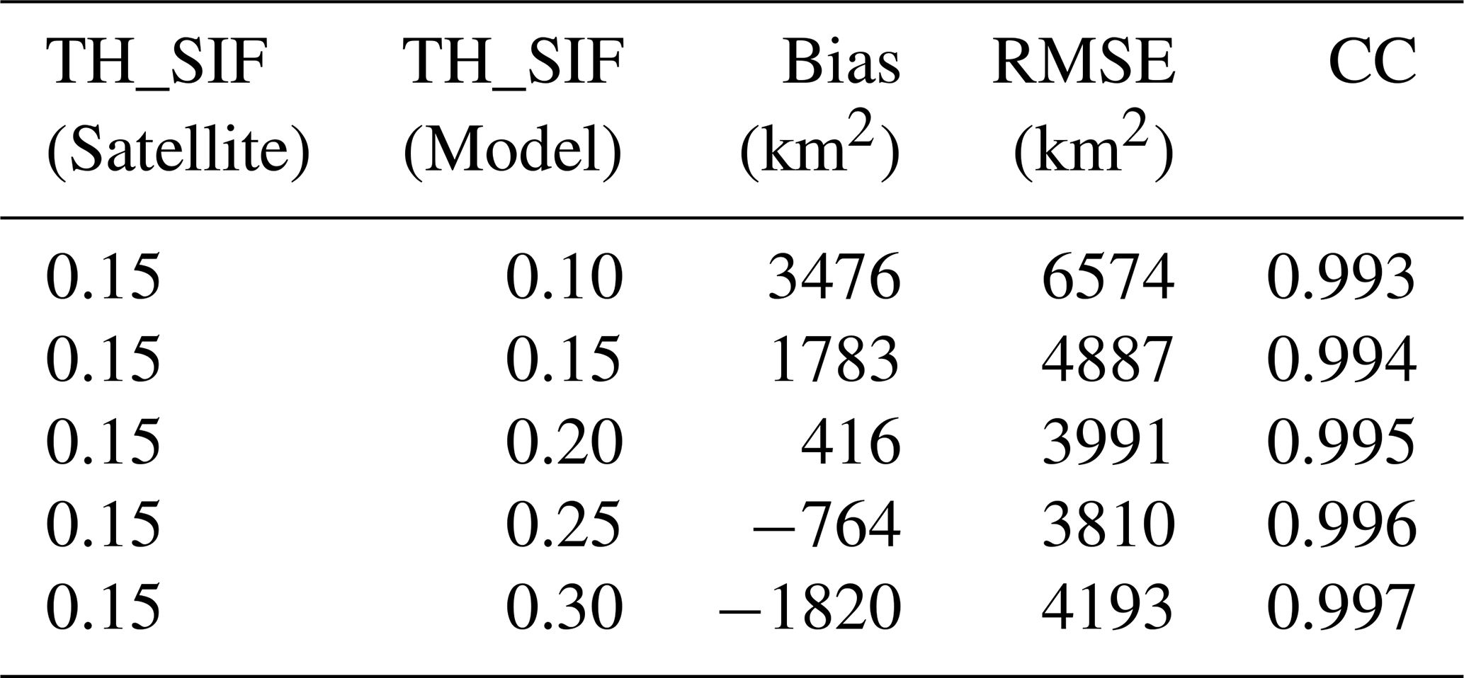
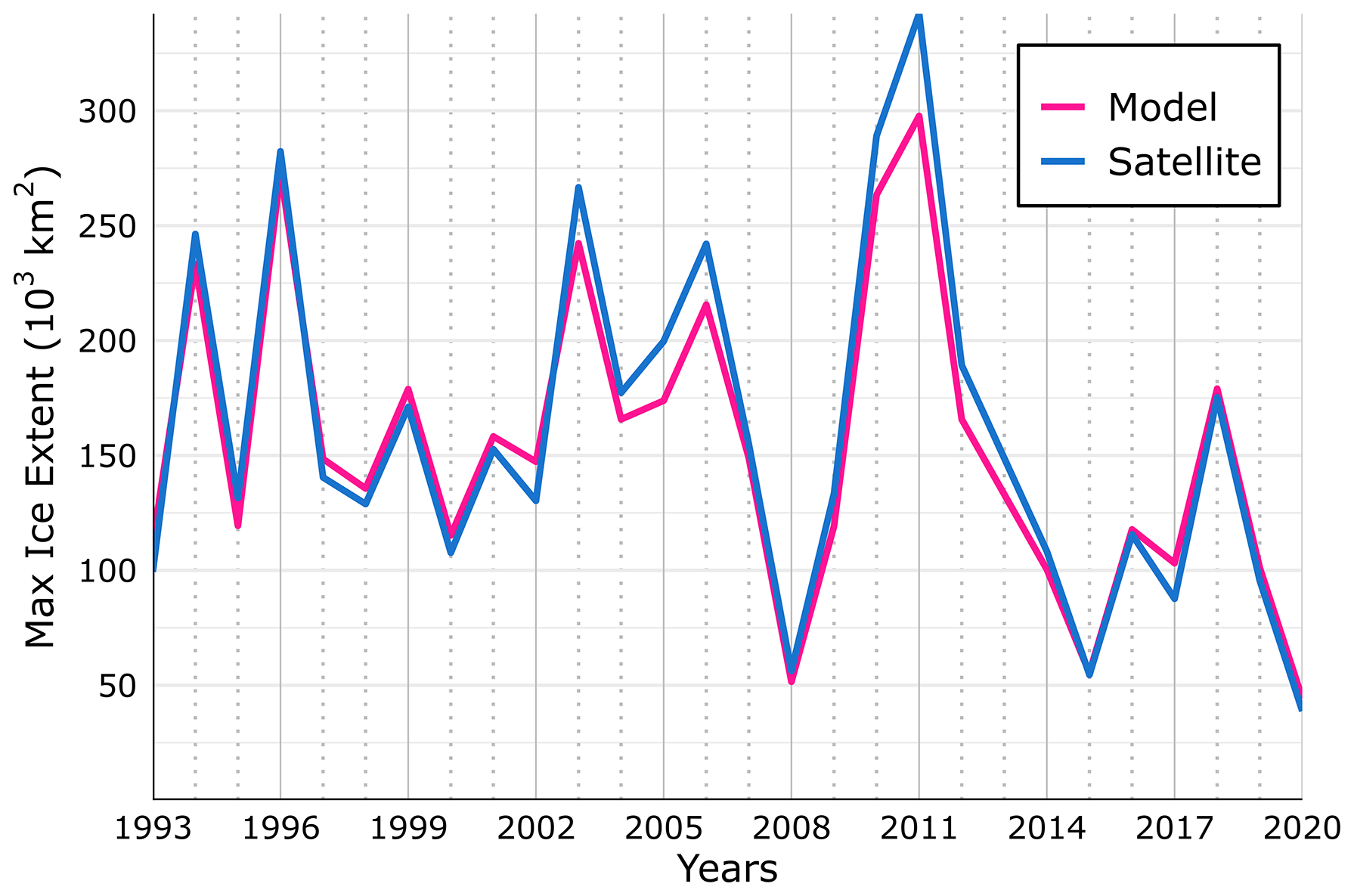
Figure 3 Time series of maximum sea ice cover extent (in 10³ km²) in the Baltic Sea across years (1993 to 2020): A comparison between Model (TH_SIF 0.20) and Satellite (TH_SIF 0.15) datasets.

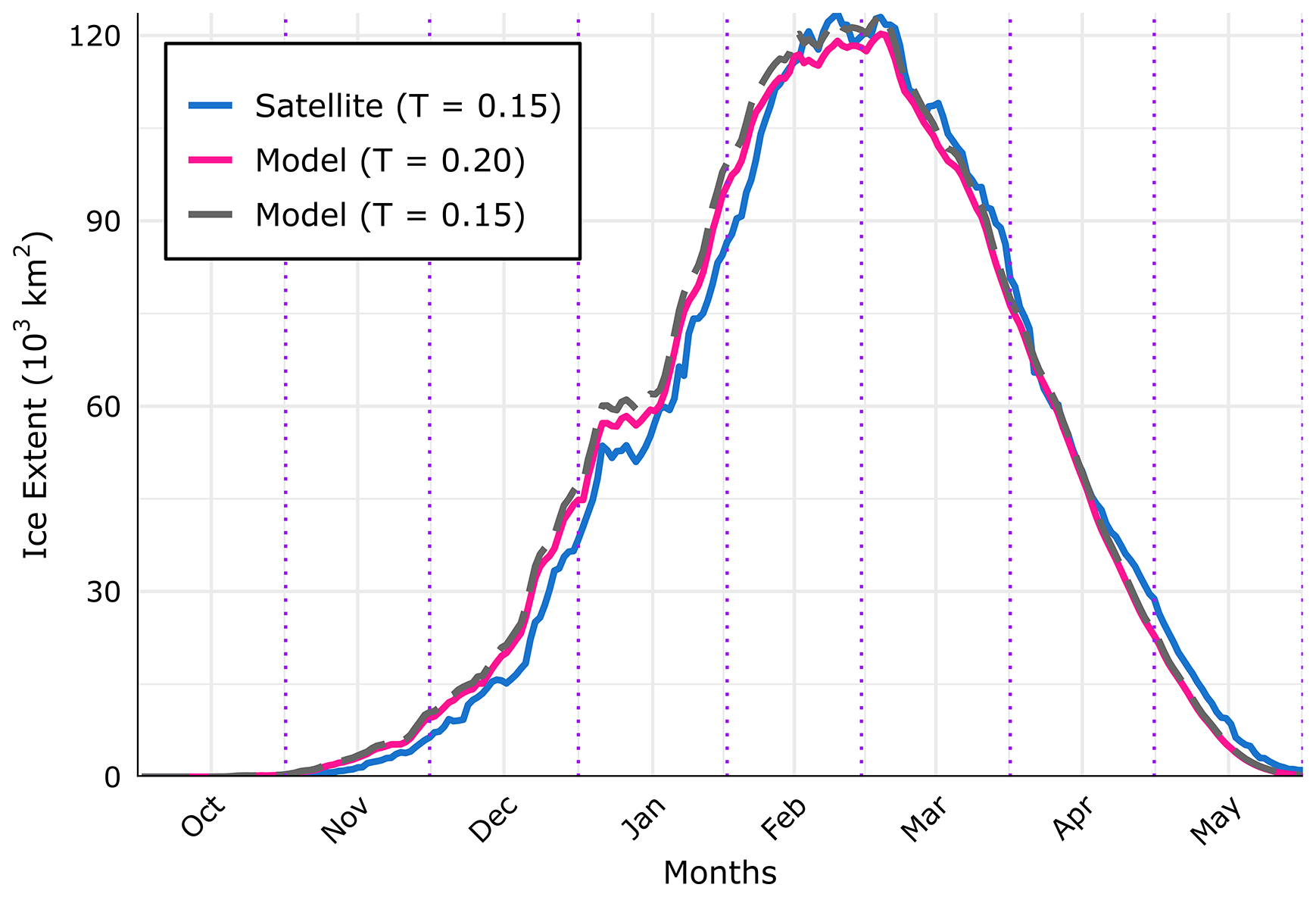
Figure 4 Sea ice season evolution of daily mean sea ice extent (in 10³ km²) in the Baltic Sea (1993/94 to 2020/21): A comparison of Model (TH_SIF 0.20) and Satellite (TH_SIF 0.15) datasets.

The set of SIE estimations was calculated from the model dataset using different SIF_TH and compared to the satellite dataset by means of robust statistics (Table 1). Bias is used as the primary criteria to select optimal threshold, RMSE and CC are calculated to confirm the results. The correlation coefficient values for all the estimations are very high, hence, we focus on the combination that shows the lowest Bias, which happens to be the combination with a sea ice fraction TH_SIF value of 0.20 for the model dataset and 0.15 for satellite observations. This combination of TH_SIF for the datasets shows the minimum bias of 416 km² and the second–lowest RMSE value at 3991 km², in close affinity to the lowest RMSE value (Table 1). The selection is based on traditionally used ice fraction thresholds, typically in increments of 0.05, such as 0.15 and 0.20, especially considering 0.20 gives reasonably low bias.

Using TH_SIF of 0.20 may not serve as the optimal approximation for the maximum extent, but we sought to assess its effectiveness in approximating the maximum extent on an interannual scale. This analysis involved plotting the annual maximum ice extent for each year within the study period (Fig. 3). When comparing maximum SIE time series, the bias between the satellite TH_SIF of 0.15 and the model TH_SIF of 0.15 is -1165 km² while the bias between the satellite TH_SIF of 0.15 and the model TH_SIF of 0.20 is −5552 km². Hence TH_SIF of 0.15 for the model dataset, provides more accurate estimates of maximum SIE, while TH_SIF of 0.20 is more suitable for temporal characteristics of the ice season, which is the primary focus of the study, and hence TH_SIF of 0.20 is used for further analysis in the subsequent sections. Despite its shortcomings, this specific combination still exhibits relative consistency in approximating the maximum extent values across the inter-annual scale (Fig. 3). We have used some sea ice season parameters in the subsequent Sect. 4.2 (these parameters have already been defined in the methodology section) to further strengthen our understanding between the two datasets and find out the disparities after using the more suitable TH_SIF for model reanalysis dataset to better depict the satellite observed sea ice season characteristics in the Baltic Sea.

4.1.2 Sea Ice Thickness

The ice thickness data from the model have been compared against SAR image & ice chart based level ice thickness for three available ice seasons (2018/19, 2019/20 and 2020/21). The comparison (Fig. 5) shows that the model total ice thickness is 1.814 times of the SAR image & ice chart based level ice thickness (with a high correlation value 0.936), which is consistent with the earlier studies (Ronkainen et al., 2018) and the product QUID file. This factor is uniform across different thickness ranges. The model has higher ice thickness more offshore than near the coasts (Fig. 5 subplot) where there is level landfast ice. The agreement between the model's total ice thickness and SAR & ice charts based level ice thickness is good and in line with earlier studies, hence the model ice thickness data (which is consistent and available for the whole study duration) has been used for further analysis.

One of the drawbacks of this analysis is the limitation in data availability, which restricts the comparison of ice thickness to only three winters. It's worth noting that the model reanalysis sea ice thickness data for these three years exhibits considerable variations, with the probability distribution plot (not shown) indicating a similar thickness distribution when compared to the complete 27-year reanalysis dataset.

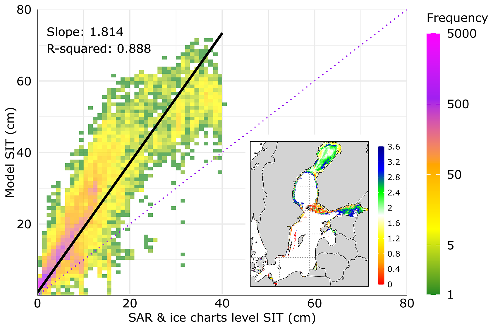
Figure 5 Time averaged sea ice thickness (in cm): SAR & ice charts based level SIT vs model based total SIT. The subplot shows the ratio of time averaged total ice thickness from model to the level ice thickness from SAR & ice charts.

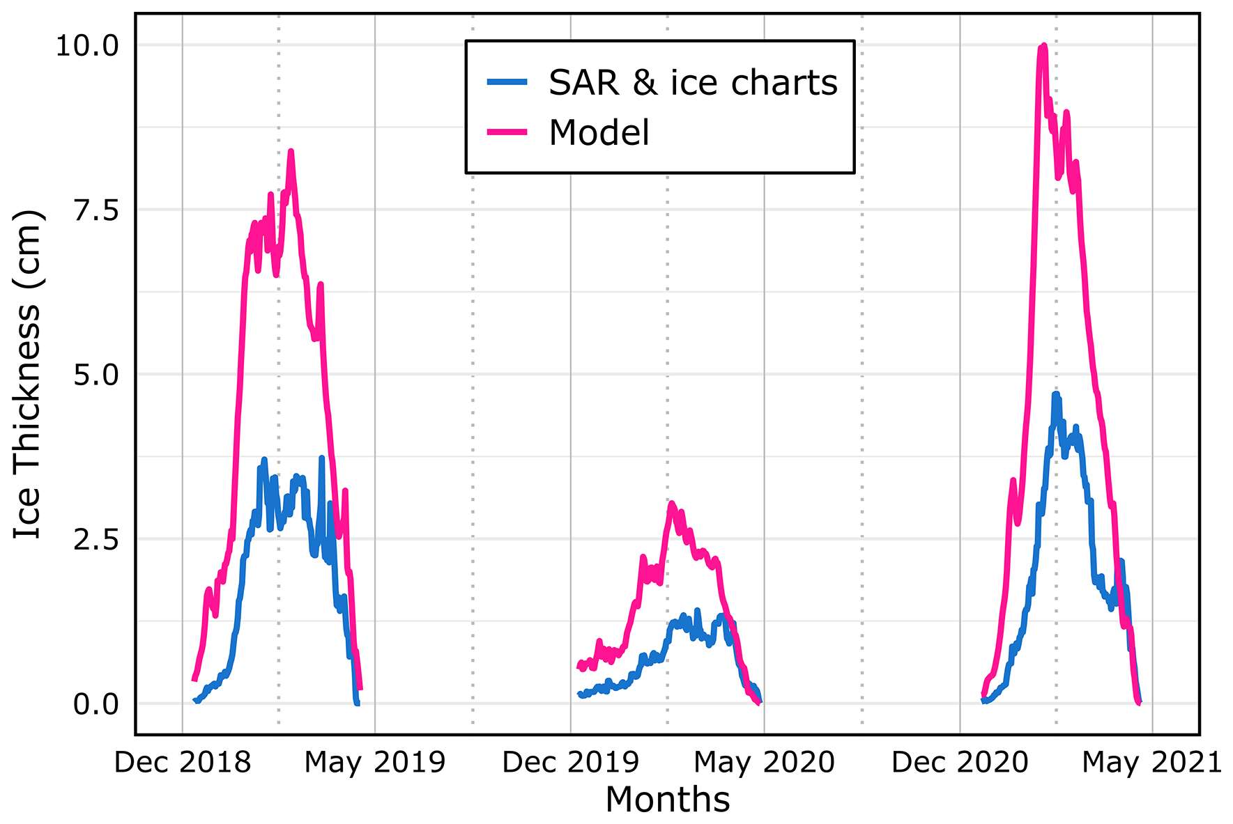
Figure 6 Time series of spatially averaged model SIT and SAR & ice charts based level ice thickness over the Baltic Sea.

4.2 Sea Ice Days Characteristics: Satellite vs Model Dataset

The spatial distribution of temporal characteristics of the Baltic Sea ice climatology are shown in Fig. 7 and a summary of each sub-basin in Table 2. Until the end of December, sea ice is predominantly observed in the northern BB sub-basin (Fig. 7a), and it persists up to May in the northernmost parts (Fig. 7d), resulting in an ice season that lasts approximately 5–6 months in that region (Fig. 7g). Hence, these parts have the largest sample size of the sea ice data for the analysis (Fig. 2a). The sea ice was observed during nearly all the years of the study period for the BB and the eastern GoF sub-basin (Fig. A1). The Bias correction is helpful in correcting or minimizing these errors. For the sea ice, bias correction has been mostly focused on correcting the total sea ice area or extent (Fučkar et al., 2014; Krikken et al., 2016). Bias correcting the models to improve their predictive capabilities of the Baltic Sea ice becomes important for all the winter activities (mentioned in Introduction) in the region. For example, Pärnu Bay and the region between Estonia and its two major islands, have a longer sea ice season compared to the nearby areas (Fig. 7g). Except for a few years, the sea ice has also been consistently present (more than 80 % of the years) in these parts (Fig. A1).

The differences between model and satellite show high spatial variability, specifically in the FD estimates. The model consistently estimates that sea ice starts to form earlier in most parts of the Baltic Sea compared to satellite data (Fig. 7c). This discrepancy is particularly pronounced in the BB, GoF, and GoR sub-basins. On the other hand, the model dataset is more accurate in estimating the end of the sea ice season (Fig. 7f). Modeled LD align better with satellite observations when compared to the FD estimates (Fig. 7f, Table 2). Therefore, earlier FD estimates are causing the overestimation in the modeled TD. The largest discrepancies in TD, similar to the FD between model and satellite, are in the BB and GoF sub-basins (Fig. 7i).

Table 2 Comparative Analysis of Satellite and Model Parameters in Baltic Sea sub-basins. The table compares parameters–FD, LD, TD, and ND–across distinct sub-basins in the Baltic Sea region.

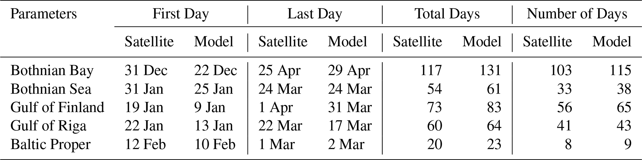
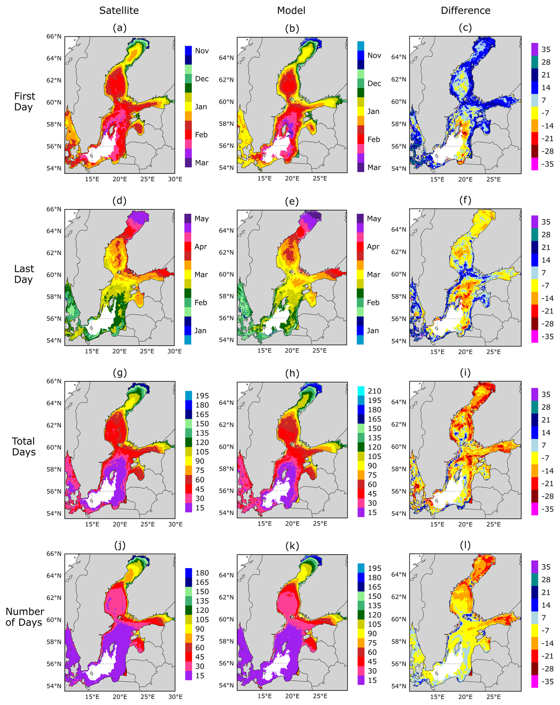
Figure 7 Map distribution of the ice season parameters, the FD of sea ice (a, b, c), the LD of sea ice (d, e, f), the TD of sea ice (g, h, i) and the ND of sea ice (j, k, l). The panels on the left column (a, d, g, j) are from the satellite dataset, the panels in the center column (b, e, h, k) are from the model dataset, and the panels on right column (c, f, i, l) are the differences of the model values from the satellite.

The ND of the sea ice differs the most from TD in the BS and BP sub-basins (Fig. 7g, j), as it depends on the sea ice dynamics within the ice season, such as sea ice drift. The ND disparities between datasets (Fig. 7l) show that the BB and GoF sub-basins exhibit the largest differences. The basin specific ice temporal characteristics (Table 2) are calculated by horizontally averaging sea ice day parameters over the regions shown in Fig. 1. The FD average has a consistent 9–10 d offset towards the early onset date in the model within the BB, GoF, and GoR sub-basins compared to satellite FD. When considering the LD across datasets, a somewhat consistent pattern of ±5 d difference is evident. Consequently, the TD exhibits the most pronounced differences in the BB and GoF sub-basins reaching 14 and 10 d respectively, meanwhile, the BS sub-basin exhibits a noticeable 7 d difference. The ND of sea ice has the largest differences of 12 and 9 d in the BB and GoF sub-basins as well. Therefore, the model consistently overestimates the ice season, mostly due to its tendency to estimate an earlier onset of the ice season.

Contrary to other sub-basins, GoR sub-basin does not display significant discrepancies in ice season length between the two datasets, owing to the model's estimates indicating a forward shift in both the FD and LD of the sea ice season. In line with trends observed in other parameters, the ND of the sea ice value exhibits the highest differences in BB and GoF sub-basins of 12 and 9 d respectively, while the other sub-basins indicate a closer resemblance between the model dataset and satellite observations for the parameter.

4.3 Sea Ice Fraction and Sea Ice Thickness Changes: Model Dataset

Based on the regime shift detected by Pärn et al. (2022) we split our study period into two parts: 1993/94–2006/07 (preceding period) and 2007/08–2020/21 (recent period), which allows us to analyze how the sea ice characteristics had changed in these periods. The average max extent has been less in the recent period, and the length of the ice season has also been shorter compared to the preceding period in the Baltic Sea (Fig. 8). The max SIE has decreased from approx. 141×10³ km² during the preceding period to 109×10³ km² in the recent period (Fig. 8).

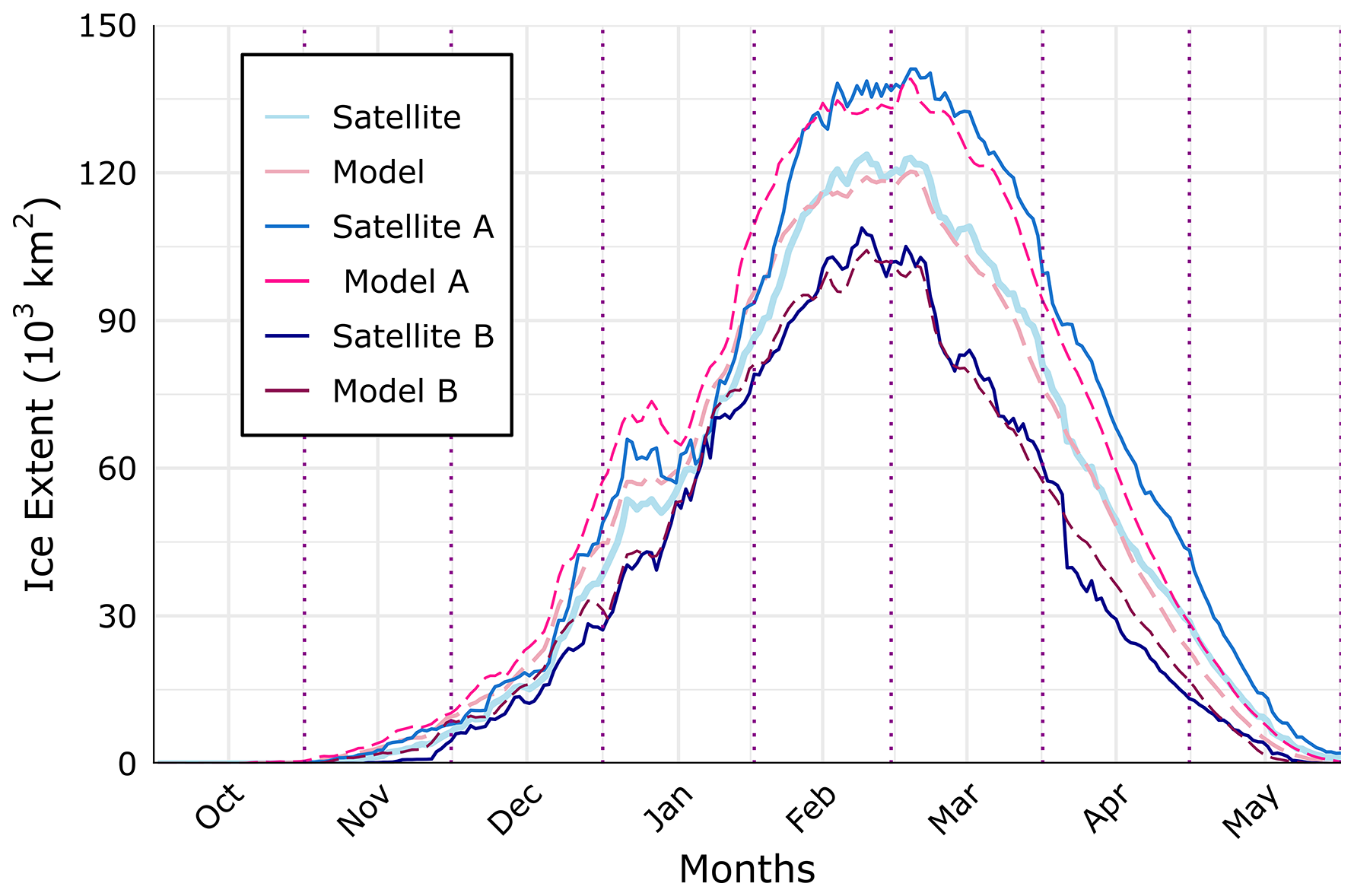
Figure 8 Sea ice season evolution of daily average Baltic Sea ice extent (in 10³ km²) from 1993/94 to 2020/21: Model (dashed) versus Satellite (solid) datasets, Assessing three periods 1993/94–2006/07, 2007/08–2020/21 (referred as A and B respectively), and the complete 1993/94–2020/21 period.

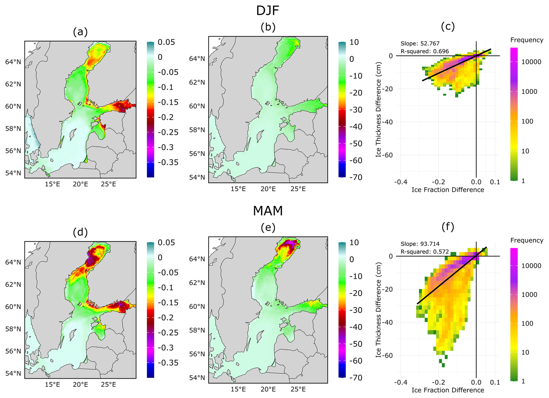
Figure 9 The changes of the SIF and SIT during the recent period 2007/08–2020/21 compared to preceding period 1993/94–2006/07, Panels (a) and (d) show the sea ice fraction (SIF) differences; (b) and (e) the sea ice thickness differences (SIT, in cm); while (c) and (f) shows the 2D histograms plotted for the fraction vs. thickness differences, shaded according to their frequency. Linear regression lines are plotted along with their respective slope and R-squared values. Upper panels are for the winter season (DJF), and lower panels are for spring season (MAM).

Table 3 sub-basin averaged values of Ice Fraction and Ice thickness for both the periods (A & B) during the winter season (DJF) and the spring season (MAM). Within the table context, A refers to the preceding period (1993/94–2006/07), while B represents the recent period (2007/08–2020/21).

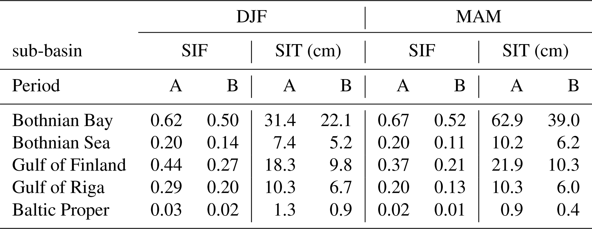
Table 4 Changes in sub-basin averaged values of Ice Fraction and Ice thickness in the recent half compared to the preceding during the winter season (DJF) and the spring season (MAM).

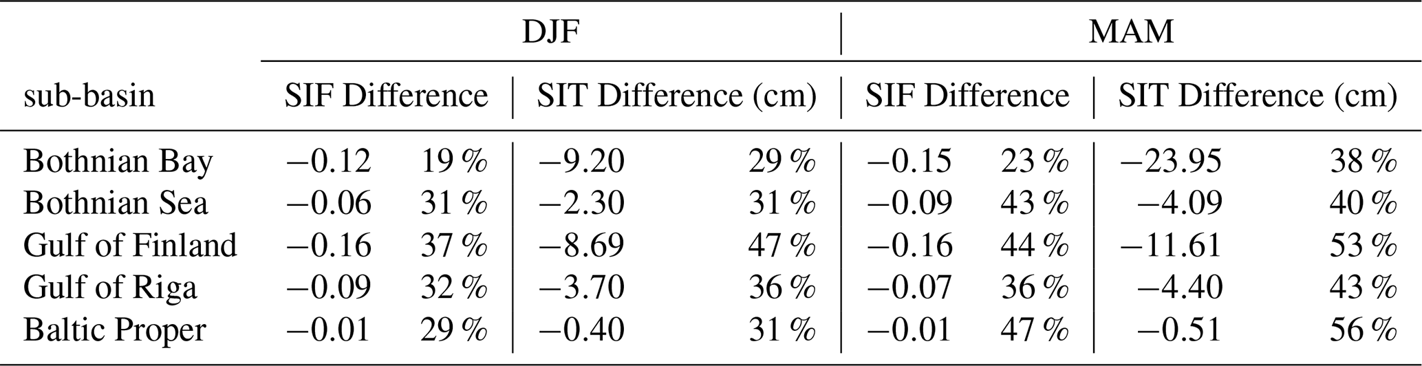
The decrease in SIE is more prominent during the spring season (after the peak SIE), as compared to the winter season (before the peak SIE) (Fig. 8). Hence we have studied the ice season characteristics during the winter season (DJF) and the spring season (MAM) separately. The date of maximum SIE day varies from year to year, however, its date fluctuates around the end of February to the beginning of March (Fig. 4). Ice fraction and thickness decreases are higher in the recent period during the spring season compared to the winter season, specifically in the BB sub-basin (Fig. 9d, e).

The coherence of the SIF and SIT changes has been shown for the winter and spring seasons in Fig. 9c and f. Although the R-squared value for both regression lines (which shows how well the data points fit the regression line) is not significant, it still provides us with some surface level information on the sea ice characteristics of the Baltic Sea. The slopes of regression lines suggest that ice thickness has generally decreased more rapidly with a decrease in ice fraction during the spring season as compared to the winter season. From the approximated slopes of regression lines (cm per % of fraction), mean ice thickness decrease during the spring season is approximately 0.94 cm as opposed to a decrease of 0.53 cm for winter season per % change of fraction (Fig. 9c, f).

The sea ice fraction values and their decline in recent period show similar trends for both of the ice season phases (Table 3). Concerning sea ice thickness, the spring season displays higher ice thickness in the BB sub-basin during the preceding period and notably the most substantial decrease in the sub-basin (Fig. 9e). This occurrence could be attributed to the presence of thicker ice in the BB sub-basin during the spring season, which could explain the pronounced reduction in ice thickness observed in that area. In percentage terms, even though the spring season exhibits thicker ice during the preceding period (making it a larger reference value for percentage change), a higher thickness decrease of 38 % during the spring season compared to a 29 % decrease during the winter season in the BB sub-basin is observed. The spring season has seen a larger decrease of ice fraction and ice thickness compared to the winter season across all the sub-basins, with the most significant being in the GoF sub-basin, where during the spring season, the ice thickness has reduced to less than half of its value (Table 4). Although our study has not focused on the underlying reasons for these changes, it is evident that recent research has detected rapid warming during the spring season (Pärn et al., 2022). Given that the GoF is a shallow basin, this warming could have contributed to the significant reduction in sea ice observed during the spring season. The BP and GoR sub-basins changes reflect the changes in a limited number of winters (Fig. A1) and consequently, particularly in the BP sub-basin, there is a significant reduction in sea ice percentage-wise, but in absolute terms, the decrease is relatively insignificant (Table 4).

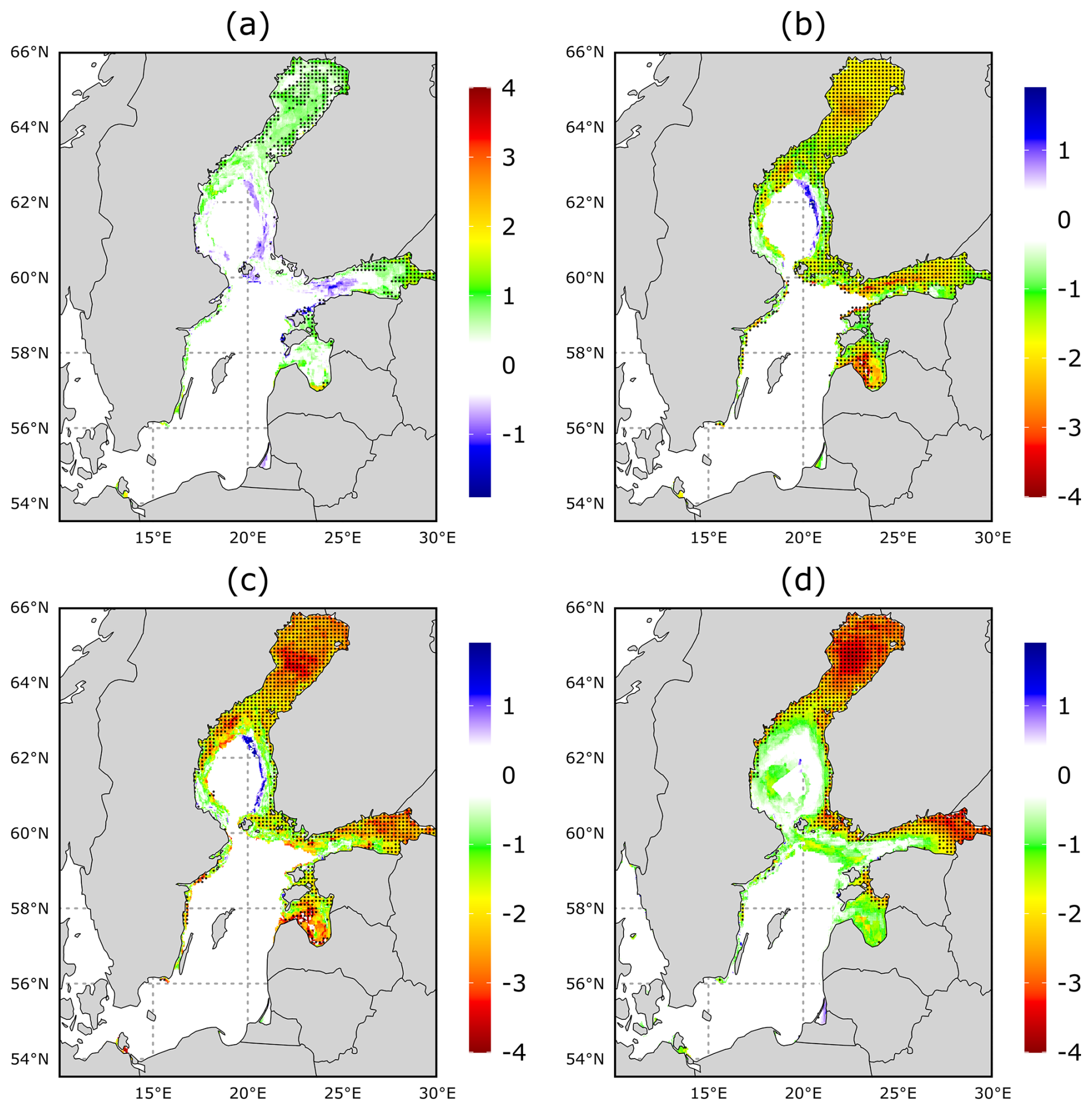
Figure 10 Linear trend for (a) FD, (b) LD, (c) TD and (d) ND of sea ice (in d yr⁻¹) during 1993/94 to 2020/21 ice seasons. Black dots mark the areas with 95 % significance level.

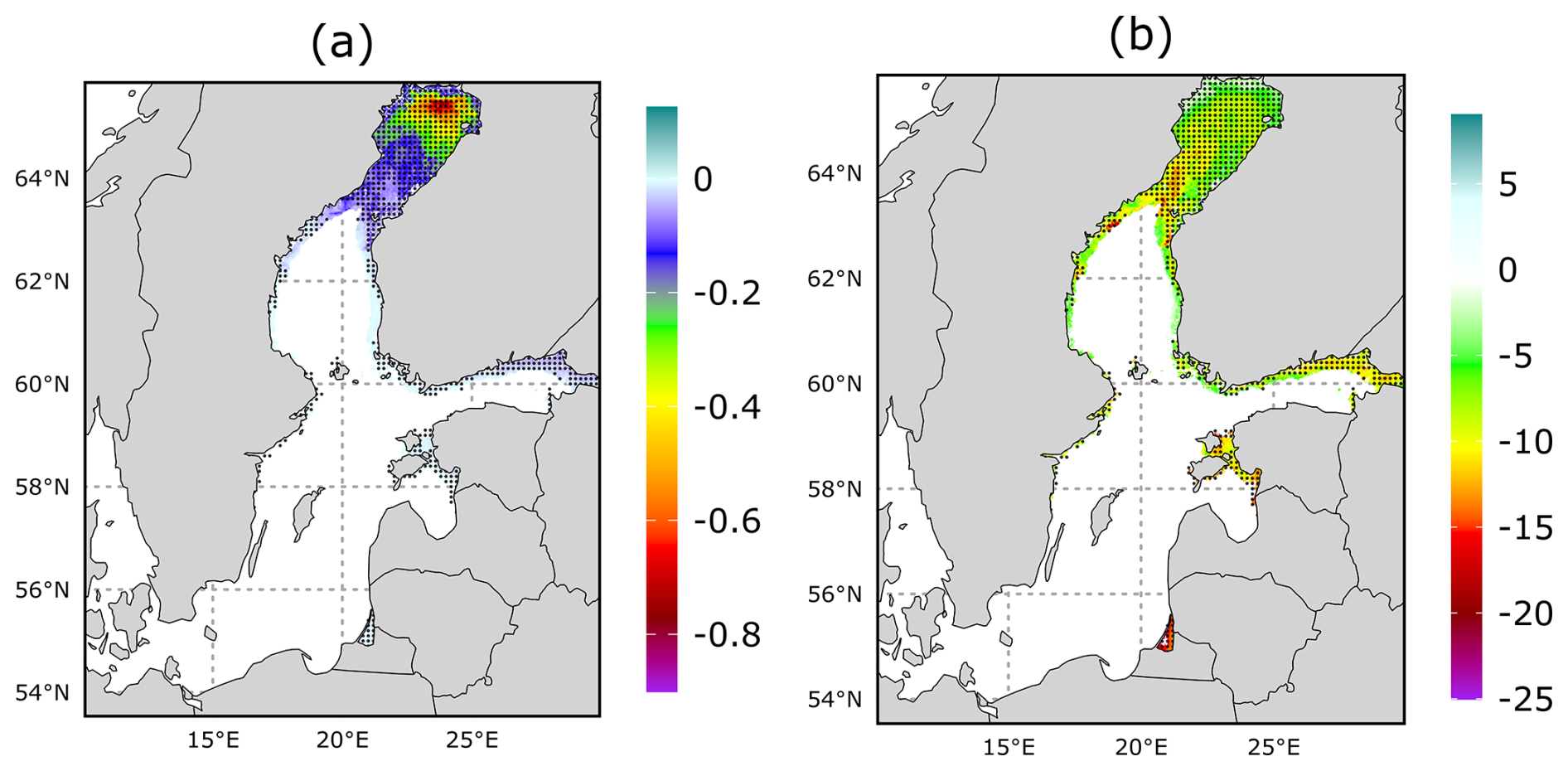
Figure 11 Linear trend for (a) ice thickness (in cm yr⁻¹) (b) ice thickness (in %) for mean of November–May ice thickness from 1993/94 to 2020/21. Black dots mark the areas with 95 % significance level.

4.4 Trend analysis of sea ice characteristics

A linear trend analysis has been performed on each grid cell of the Baltic Sea over the study period for the parameters FD, LD, TD, ND of sea ice and the ice thickness. The resulting spatial distributions of the linear trend across the Baltic Sea are shown in Figs. 10 and 11. The FD of sea ice in the Baltic Sea shows an increasing trend, which is statistically insignificant at 95 % significance level for the most parts of the Baltic Sea (Fig. 10a). However, in the case of the LD of sea ice, a decrease of approximately 1–2 d yr⁻¹ above 95 % significance level is observed in almost all parts of BB sub-basin area and in some parts of the GoF sub-basin as well (Fig. 10b). Hence, a decrease of approx. 1–3 d yr⁻¹ in TD and ND of sea ice parameters is observed in roughly the same areas. The linear trends of the annual mean ice thicknesses averaged over ice season (November to May) show that the areas of the northern BB sub-basin have the highest and most significant (over 95 % significance level) decreasing trend of order up to approx. 0.7 cm yr⁻¹ (Fig. 11a). The BB has the highest thickness of sea ice across all the sub-basins (Table 3). The linear trends that are normalized with their respective mean ice thickness show the ice thickness trend in terms of average percentage decrease. The normalized trend values have been uniform over the BB sub-basin standing at approximately −5 %.

5 Discussion

Bias correcting the models to improve their predictive capabilities of the Baltic Sea ice becomes important for all the winter activities in the region. For the sea ice, bias correction has been mostly focused on correcting the total sea ice area or extent (Fučkar et al., 2014; Krikken et al., 2016). In our study the latest Copernicus Baltic Sea Physics reanalysis product is bias corrected (using a different SIF threshold value) for the mean season evolution of the sea ice extent. For sea ice thickness, satellite product also has uncertainties, and the ice maps only take into account the visible ice thickness from ships when estimating offshore ice thickness. Moreover, they do not contain the additional volume of deformed ice (Raudsepp et al., 2019). Using the SAR imagery & ice charts based Copernicus product for ice thickness could be more suitable, however, it is only available from 2018 onwards. Hence, the model ice thickness was used for the analysis.

In the study by Jevrejeva et al. (2004), the long-term time series of date of freezing, breakup, number of days with ice, and maximum annual ice thickness of landfast ice in the Baltic Sea were examined using the station data, and the results provided insights into complicated variability in ice conditions. Their 100 year time series showed a general trend toward reduced ice conditions, with the largest change being the length of the ice season, which has decreased by 14–44 d during the 20th century. Instead of station data (which are mostly onshore), the satellite data provide coverage over the whole Baltic Sea, where we observe a reduced ice season length (on average approx. 1–3 d yr⁻¹) and decreased maximum SIE (by approx. 32×10³ km²) in the recent period (2007/08–2020/21) of our study. As compared to the Jevrejeva et al. (2004) where most of ice season length analysis was done for coastal locations, the current study extends that knowledge to offshore areas as well, for the period 1993/94–2020/2021. The highest reduction in the ice season is also observed at the offshore areas.

Our analysis confirms that the maximum sea ice extent (SIE) in the Baltic Sea typically occurs in late February to early March, consistent with previous findings (BACC II Author Team, 2015). Given that the most significant reductions in SIE occur after this peak, we performed a seasonal comparison by analyzing changes separately for the winter (DJF) and spring (MAM) periods.

A common trend observed is that both the sea ice fraction (correspondingly sea ice extent) and sea ice thickness have decreased in the recent period during both of the ice season phases, specifically, the changes are larger during the spring season, which is in line with the study by Pärn et al. (2022), where they have observed a regime shift during spring time beginning in 2008 in all the basins of the Baltic Sea. For the BB sub-basin, the reduction in sea ice thickness during the spring season is more pronounced in absolute terms compared to the decrease in sea ice fraction in the study. The possible causes could be partly attributed to higher sea ice thickness values in the BB during the spring season in the preceding period of the study. There was no general conclusion concerning maximum annual ice thickness from Jevrejeva et al. (2004), while some sites (Kemi and Kihnu) showed an increase, most time series were characterized by a decreasing trend. During our study period, we observed a significant uniform decreasing trend (about 5 %) in the mean SIT on the northern BB sub-basin, reaching up to 0.7 cm yr⁻¹ in some parts. The value is dependent on the months selected for the annual ice thickness mean.

5.1 Physical Mechanisms of Observed Sea Ice Decline

Climatic conditions during the winter months (December–February) largely control the development of the ice cover in the Baltic Sea (Omstedt and Chen, 2001). The reduced ice conditions trends in the Baltic Sea during the 20th century were also related to a warming trend in winter air temperatures over Europe (Jevrejeva et al., 2004). The warming from the present climate leads to a decrease in ice extent by 35–40×10³ km² °C⁻¹ air temperature change (Leppäranta, 2023). The average air temperature during the study duration has decreased approx. 0.6–0.7 °C (Source: NASA/GISS; https://climate.nasa.gov/vital-signs/global-temperature/, last access: 15 January 2025), and the average max extent has decreased from approx. 141×10³ km² (33.6 % of the total Baltic Sea) during the preceding period to 109×10³ km² (25.9 %) during the recent period.

During spring, when incoming solar radiation rapidly increases, the pronounced decline in sea ice extent and thickness across the Baltic Sea reflects a complex interplay of regional warming, feedback mechanisms, and atmospheric circulation. One key driver is the albedo feedback, where reduced spring snow and ice cover lowers surface reflectivity, increases solar absorption, and accelerates ice melt (Granskog et al., 2006; Vihma and Haapala, 2009). The earlier melt onset observed in the latter half of the study period – evident in the shift of peak sea ice extent to earlier dates (from approx. 3 March in 1993–2007 to 22 February in 2008–2021) – supports this mechanism and suggests a shortening of the effective ice season. This pattern aligns with findings by Perovich et al. (2007), they demonstrated that the amount of solar radiation absorbed at the ice surface is strongly correlated with the timing of melt onset, reinforcing the role of albedo feedback in amplifying early spring melting.

Sub-basin differences further indicate the role of regional oceanographic and climatic variability: the Bothnian Bay, with typically thicker and longer-lasting ice, shows larger absolute reductions in sea ice thickness, while the Gulf of Finland – being shallower and more influenced by atmospheric forcing – exhibits more pronounced relative declines (Leppäranta and Myrberg, 2009; Omstedt and Chen, 2001).

Importantly, interannual variability in winter ice conditions is strongly modulated by large-scale atmospheric circulation. The winter (DJF) North Atlantic Oscillation (NAO) and Arctic Oscillation (AO) indices (obtained from NOAA's Climate Prediction Center, https://www.cpc.ncep.noaa.gov/products/precip/CWlink/daily_ao_index/history/method.shtml, last access: 15 January 2025) exhibit significant negative correlations with maximum sea ice extent over the study period (r=−0.62 and −0.71 respectively, excluding 2013). This confirms that positive NAO and AO phases, which enhance westerly winds and heat transport over northern Europe, are associated with milder winters and suppressed sea ice growth in the Baltic Sea (Jevrejeva, 2001; Jevrejeva et al., 2004; Vihma and Haapala, 2009; Leppäranta and Myrberg, 2009).

5.2 Implications for Sea Ice Modeling and Improvements

Parametrization of sea-ice processes is critical for accurately simulating ice evolution, especially in marginal seas like the Baltic Sea. A sensitivity study by Nie et al. (2023) using the NEMO4.0–SI³ model showed that sea ice concentration and volume are strongly influenced by snow-related thermodynamic processes and the number of ice thickness categories, while albedo-related parameters had comparatively minor impact in the Southern Ocean. In the Baltic Sea, however, our results highlight that springtime thinning is disproportionately stronger than wintertime changes, suggesting that snow–ice thermodynamics and thin-ice growth regimes may be particularly relevant here. In fact, sea-ice variability in the Baltic Sea is more closely tied to local seasonal ice thickness, particularly in thin-ice growth regimes influenced by both thermodynamic and dynamic processes (Pemberton et al., 2017). Although often underrepresented in large-scale models, regionally and seasonally variable sea-ice and snow albedo can be important, especially in transitional zones, as shown by observational studies in the Arctic (Light et al., 2022) and the Baltic Sea (Pirazzini et al., 2006). This aligns with our finding of earlier melt onset and enhanced spring albedo feedback, underscoring the need to better capture snow and thin-ice processes in regional models.

Discrepancies in sea-ice model performance can arise from both inaccuracies in atmospheric forcing and uncertainties in the parameterization of ocean–ice–atmosphere interactions (Vihma and Haapala, 2009). Most state-of-the-art models still lack a fully coupled atmosphere–wave–ice–ocean framework, relying instead on simplified approximations and corrections introduced via data assimilation. For example, in the Nemo–Nordic 2.0 model, assimilation of satellite sea surface temperature (SST) reduces SST bias but fails to fully correct the timing of ice onset, which remains delayed by approximately a week (Fig. 8c). This may indicate unresolved errors in ocean surface cooling or deficiencies in early ice formation processes. Given that Baltic Sea ice dynamics differ significantly from polar regions – most notably due to the absence of multi-year ice – bulk parameterizations for thermodynamics and rheology should be revised for regional conditions, and models calibrated against high-quality observational datasets (Pemberton et al., 2017). As fine-resolution models are increasingly applied to dynamically active regions, implementing more advanced rheology schemes, such as brittle-ice formulations, may also become necessary (Brodeau et al., 2024; Olason et al., 2022).

Accurately representing wave–ice interactions has likewise become increasingly important, particularly in the marginal ice zone (MIZ), where waves influence ice breakup, drift, and thermodynamic processes (Sutherland and Dumont, 2018). Studies across global and regional Arctic and Baltic domains have shown that coupling sea-ice or ocean models with wave dynamics –especially with prognostic floe-size or floe-size/thickness distributions – substantially enhances simulations of ice–ocean interactions. Wave-induced fracturing increases exposed ice perimeter and lateral melt (Roach et al., 2018), while floe-size distribution amplifies ice–ocean heat fluxes despite counteracting atmospheric and oceanic feedbacks (Yang et al., 2024). Additional observational and modeling work highlights the role of wave penetration and storm-driven upper-ocean mixing in driving rapid ice loss (Kohout et al., 2014; Blanchard-Wrigglesworth et al., 2022), along with secondary effects such as wave-enhanced surface warming, altered stratification, and upwelling via Stokes–Coriolis forcing in the Baltic Sea (Alari et al., 2016). For our study region, where thinner and more fragile spring ice has been increasingly observed, the influence of waves on breakup and lateral melt may become more pronounced in future conditions and should be considered in model development.

Despite these advances, fully integrated ocean–ice–wave–atmosphere coupling remains uncommon and under development. Most models continue to couple only subsets of the system – such as atmosphere–wave–ocean (Grayek et al., 2023), wave–sea ice (Boutin et al., 2020), ocean–wave (Couvelard et al., 2020), or atmosphere–ocean–wave–sea ice with floe-size dynamics (Yang et al., 2024) – while gradually advancing toward more comprehensive frameworks. In recognition of this, the CMIP7 Data Request: Ocean and Sea Ice Priorities and Opportunities identifies wind waves as a priority science use case, aiming to improve understanding of how wave-driven processes affect sea ice and ocean variability (Li et al., 2025). This underscores the need for fully coupled sea-ice–wave models in next-generation Earth system simulations.

Remaining uncertainties in such coupled models can be significantly reduced through multivariate data assimilation. For the Baltic Sea, Axell and Liu (2016) demonstrated that assimilating sea ice concentration, thickness, and drift into a coupled ice–ocean model notably improved the representation of ice conditions, particularly when multivariate corrections were used to propagate observational information across model variables. More broadly, sea ice assimilation methods such as nudging, optimal interpolation, and ensemble-based techniques (e.g., Ensemble Kalman Filter) are increasingly used to integrate sea ice concentration, thickness, drift, and in some cases snow depth (Zhang et al., 2018; Blockley and Peterson, 2018; Koldunov et al., 2017). Assimilation of snow depth can further improve snow state estimation, though effects on long-term sea-ice forecasts remain mixed (Fritzner et al., 2019). Additionally, assimilating indirect ice parameters, such as ice-edge position or ridged area, has been shown to enhance the representation of dynamic and volumetric ice properties (Prasad et al., 2021). Overall, these studies suggest that using assimilation of both direct sea-ice properties (extent, thickness, drift) and indirect parameters (e.g., ice edge, ridging) could help reduce the biases we observed in our analysis.

6 Conclusion

The study focused on analyzing the Baltic Sea's ice characteristics, utilizing satellite and model datasets. The main findings from the study are given below.

• The sea ice statistics (sea ice extent, season length, and mean thickness) from the Copernicus Marine Baltic Sea Physics Reanalysis product (BALTICSEA_MULTIYEAR_PHY_003_011) have been compared with satellite and SAR & Ice charts based datasets. A sea ice fraction threshold of 0.20 for the model dataset provides the most optimal match against the satellite's 0.15 threshold, minimizing bias and root mean square error for the temporal evolution of sea ice extent over the study period.

• During the study period, the model dataset consistently predicts an earlier onset of sea ice but aligns better with satellite data regarding the end of the ice season. Notable disparities exist in the Bothnian Bay and Gulf of Finland sub-basins, where the model forecasts longer ice seasons and more sea ice days than the satellite data.

• Recent trends showcase decreasing sea ice fraction and thickness in almost every part of the Baltic Sea. Specifically in the Bothnian Bay, the spring season exhibits a more rapid decrease in ice thickness per percentage decrease in ice fraction, compared to the winter season. In the Gulf of Finland sub-basin the mean ice thickness has become less than half of its value during the spring season in the recent half (2007/08–2020/21) of the study.

• The annual mean ice thickness has been decreasing at the highest rate (in absolute terms) in the Bothnian Bay sub-basin with some northern areas reaching up to approx. 0.7 cm yr⁻¹, but relative trends of ice thickness thinning have been nearly uniform (approx. 5 %) across all of the Baltic Sea sub-basins.

Appendix A

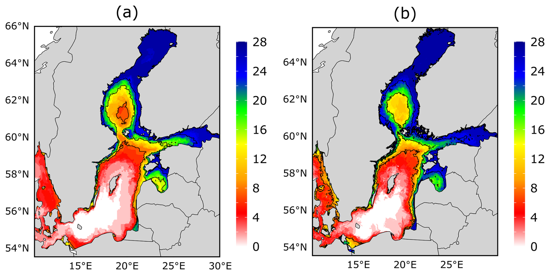
Figure A1 The sample size of the datasets used in the calculations, panels (a) and (b) illustrate the count of years factored into the calculations (solid thin black contour lines are at value of 8, 16, and 24 years) from satellite and model data respectively.