Benchmarking passive-microwave-satellite-derived freeze–thaw datasets

Satellite-derived soil surface state has been identified to be of added value for a wide range of applications. Frozen versus unfrozen conditions are operationally mostly derived using passive microwave (PMW) measurements from various sensors and different frequencies. Products differ thematically, as well as in terms of spatial and temporal characteristics. All of them offer only comparably coarse spatial resolutions on the order of several kilometers to tens of kilometers, which limits their applicability. Quality assessment is usually limited to comparisons with in situ point records, but a regional benchmarking dataset is, thus far, missing. Synthetic aperture radar (SAR) offers high spatial detail and, thus, is potentially suitable for assessment of the operational products. Specifically, dual-polarized C-band data acquired by Sentinel-1, operating in interferometric wide (IW) swath mode with a ground resolution of 5 m×20 m in range and azimuth, provide dense time series in some regions and are therefore a suitable basis for benchmarking. We developed a robust freeze–thaw (FT) detection approach that is suitable for tundra regions, applying a constant threshold to the combined C-band VV (vertically sent and received) and VH (vertically sent and horizontally received) polarization ratios. The achieved performance (91.8 %) is similar to previous methods which apply an empirical local threshold to single-polarized VV backscatter data.

All global products, tested with the resulting benchmarking dataset, are of value for freeze–thaw retrieval, although differences were found depending on the season, particularly during the spring and autumn transition.

Fusion can improve the representation of thaw and freeze-up, but a multi-purpose applicability cannot be obtained since the transition periods are not fully captured by any of the operational coarse-resolution products.

1 Introduction

Soil surface state (frozen or unfrozen) can be obtained from space using active microwave and passive microwave (PMW) data. Using spaceborne passive microwave data, 42 % of the Northern Hemisphere land surface has been identified to be affected by seasonal freezing and thawing (Kim et al., 2012). This includes permafrost regions, where it is a characteristic of the so-called active layer, the upper soil on top of permafrost. Satellite-derived freeze–thaw (FT) information is, hence, suitable as a proxy for permafrost characteristics (e.g., extent – Park et al., 2016b; ground temperature – Kroisleitner et al., 2018). The performance of passive microwave retrieval algorithms depends on the wavelength, the acquisition timing, and the algorithm used to derive the surface state (Johnston et al., 2020). Land cover at the subgrid scale also needs to be considered (Bergstedt and Bartsch, 2017; Bergstedt et al., 2020b).

A traditional application area of FT products is the masking of satellite-derived soil moisture, targeting a separation of the periods with and without the presence of liquid water in the upper soil. The requirements are, in such cases, usually aligned with the soil moisture product (spatial and temporal resolution). However, some of the available products lack consistent FT flagging (Trofaier et al., 2017). Further potential of soil FT products includes, for example, the assessment of the vegetation growing season (Kim et al., 2014, 2020; Park et al., 2016b; Böttcher et al., 2018), evapotranspiration (Zhang et al., 2021; Kim et al., 2018), and fluxes of greenhouse gases (Tenkanen et al., 2021; Erkkilä et al., 2023). The latter includes confining the activity period of soil microbes (Bartsch et al., 2007; Kim et al., 2014) and the combination with greenhouse gas concentrations derived from satellites and permafrost (Park et al., 2016a; Kroisleitner et al., 2018).

Different applications have different needs regarding FT detection. For example, for the climate modeling community, a frozen-fraction approach is required rather than a frozen–unfrozen classification (Bergstedt et al., 2020b). Subgrid information regarding snowmelt patterns is also of interest in the context of long-term ecosystem monitoring in the Arctic (Rixen et al., 2022). Surface state products derived by satellites represent the surface condition of either snow and ice or soils. In case of snow, the terms “wet” and “dry” or “frozen” and “melting” are used, while, for soil, the terms “frozen” and “unfrozen” are used to describe the states. Dedicated FT products mostly address soils and, thus, acquisitions under snow-free conditions, but wet-snow information is of added value for such observations due to associated changes in soil temperature beneath the snowpack (e.g., Bartsch et al., 2007; Kroisleitner et al., 2018). Climate change impact can be documented through the length of the unfrozen or snow-free season, but spring snow thaw timing and the length of the snowmelt period also need to be monitored (e.g., Kouki et al., 2019).

The production of an FT climate data record (CDR) may require the combination of products from different satellites. Differences between records using different wavelengths have been identified (e.g., Johnston et al., 2020). A range of strategies for the fusion of different records have been proposed, specifically L-band passive microwave and C-band scatterometers (Chen et al., 2019; Zhong et al., 2022). Inconsistencies and systematic differences due to acquisition timing and differences regarding the wavelength and system (active–passive; static in the beginning, varying towards the end; Trofaier et al., 2017) need further investigation. The utility of the products varies based on not only different user needs but also the retrieval approach and calibration data. Reanalysis data are commonly used to define a threshold for surface state classification; 0 °C is applied as a threshold for passive records representing the brightness temperature and reanalysis value relationship through a cosine function (Kim et al., 2014). Naeimi et al. (2012) fit a logistic function to describe the relationship between temperature and C-VV (vertically sent and received) backscatter. The turning point of the function is considered to be the threshold. Kroisleitner et al. (2018) found that the PMW-derived frozen period length differs considerably from that of Naeimi et al. (2012). Possible reasons are the acquisition time, wavelength, and calibration approach. These approaches differ from snowmelt products where, for example, in the case of sea ice, a temperature above −1 °C for 3 consecutive days is considered (Smith et al., 2022). Alternatively, over land, the condition of diurnal thawing and refreezing for the start of spring melt has been suggested, but this requires higher repeat measurement intervals than what is usually available (Bartsch et al., 2007). Most products target 80 % detection accuracy. A commonly agreed upon benchmark for this assessment is lacking so far, relating partially to the lack of representation of spatial variations by the available in situ data within the footprints.

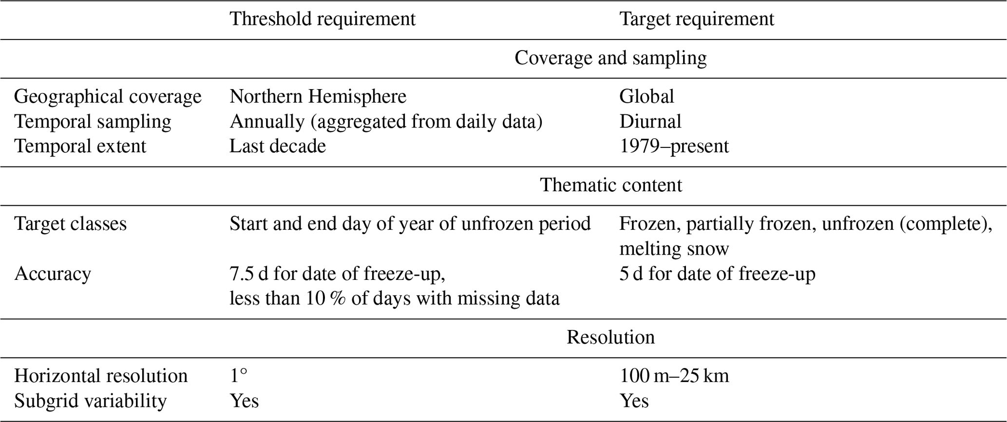
Consolidated requirements for an FT product aimed at permafrost research have, so far, only been stated in Bartsch et al. (2022). A product of 100 m spatial resolution with 10 d intervals has been requested. Kroisleitner et al. (2018), with a focus on MetOp ASCAT and SSMI, show that a daily resolution is required for ground temperature estimation. General requirements for a ground temperature product have been collected as part of the Permafrost_cci baseline project (Bartsch et al., 2023d) and need to be considered in this context. As a threshold requirement for temporal and spatial coverage, at least the last decade needs to be addressed, as well as the whole Arctic. The target should be a global product including not only the Northern Hemisphere but also mountain ranges and polar ice-free regions in the Southern Hemisphere. A threshold of 10 km resolution and a target of 1 km resolution will eventually be required to serve the needs of permafrost modeling at a global scale (Bartsch et al., 2023d).

A major challenge with coarse-resolution satellite products based on PMW data across the Arctic is the quality assessment with in situ data due to the scarce availability of ground stations and the loss of representativeness because of high landscape heterogeneity. Available FT products have a nominal spatial resolution on the order of several tens of kilometers. Bergstedt et al. (2020b) demonstrated that considerable variations can occur within a footprint due to topography and/or variability in land surface types. Another option for evaluating the quality of coarse-resolution products is using C-band-based data, which have a higher spatial resolution. So far, such investigations have been limited to C-band scatterometers, specifically the MetOp Advanced Scatterometer (ASCAT).

A strategy for SAR (synthetic aperture radar)-based benchmark dataset creation which relies on calibration with reanalysis data is described in Bergstedt et al. (2020b). This calibration approach follows the methodology proposed for scatterometers by Naeimi et al. (2012). It needs to be carried out for each footprint or pixel individually since various factors, such as surface roughness and volume scattering in the surface layer, may impact the absolute backscatter intensity values. Naeimi et al. (2012) compared gridded temperature data (ERA-Interim reanalysis data) and MetOp ASCAT C-Band VV backscatter data (grid spacing of approximately 12.5 km) and fitted a logistic curve. The lower flat part of the function represents frozen conditions, while the upper flat part relates to the unfrozen conditions. The inflection point provides the location-specific threshold. This method requires suitable temperature data for each grid point. As these data are not available at a high spatial resolution, as provided by Sentinel-1 (5 m×20 m; 10 m nominal resolution), a method independent from such parameterization needs to be developed for regional applications. An algorithm which, for example, makes use of a universal threshold is required. The study by Bergstedt et al. (2020b) was, in addition, limited to VV polarization matching ASCAT properties. Backscatter intensity, expressed as σ₀, was used, and incidence angle normalization to 40° was applied using the approach by Widhalm et al. (2018) in order to match ASCAT specifications. An overall accuracy of 94 % was obtained in comparison to soil temperature data from a tundra area. Missions such as Copernicus Sentinel-1 operate in dual-polarization mode, providing co- and cross-polarization over most land areas (commonly VV and VH – vertically sent and horizontally received). The use of both for FT has been investigated only in very few cases so far. Cohen et al. (2021) calculate the backscatter difference (for each date to be classified) with respect to a frozen and unfrozen reference (pre-selected representative scenes). The study was eventually also limited to VV as the focus was on forested environments, where VH is expected to be influenced by the canopy. σ₀ was used, and the ground and canopy contributions were separated (including consideration of incidence angle). A static but regionally specific threshold applied to the difference between the deviation from the frozen and thawed references is suggested. Similarities compared to air temperature were between 64 % and 99 % depending on the region. A further approach which has been regionally tested for Sentinel-1 is the use of a convolutional neural network (CNN) algorithm also trained using backscatter from a frozen and unfrozen reference period, using both VV and VH, as well as incidence angle and land cover information (Chen et al., 2024). A classification accuracy of 88 % was obtained in comparison to soil temperature data across an area north of the treeline where the CNN was trained.

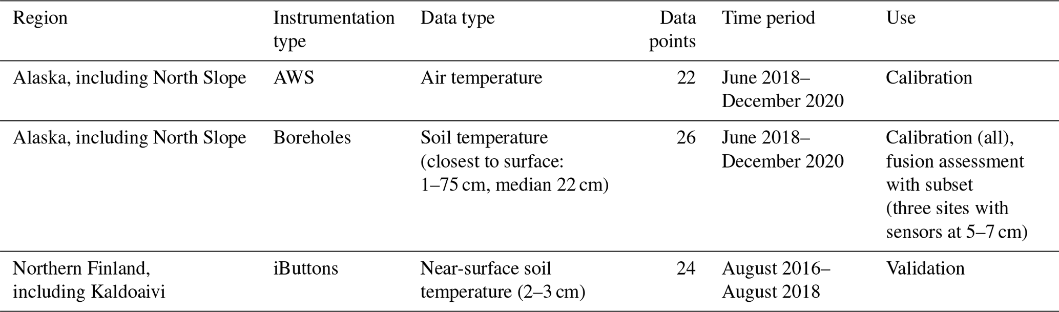
Algorithms which use backscatter ratios for wet or dry-snow detection based on Sentinel-1 exist. This allows the application of a global threshold value to distinguish between states without a location-specific parameterization, also avoiding the need to directly consider the incidence angle (Nagler and Rott, 2000). So far, the scheme has not been tested for soil FT. Previous calibration and validation activities have found that a global threshold of −2 dB (ratio between acquisition and reference image) is suitable to discriminate between wet and dry snow. It is hypothesized that a similar strategy is suitable for frozen versus unfrozen soil classification. This requires sites with good in situ data availability, which are scarce in permafrost regions. A comparably high number of borehole records are, however, available over the Alaska North Slope (Biskaborn et al., 2019). Also, measurements from an FT-dedicated sensor network are available from northern Finland (Bergstedt et al., 2020b).

The purpose of this study is to evaluate the utility of C-band SAR data available at VV and VH polarizations for the benchmarking of passive-microwave-satellite-derived freeze–thaw products which have a coarse resolution but global coverage. In situ air and soil temperature data from different locations across the Alaska North Slope are used to identify a suitable ratio threshold for the benchmark dataset creation. Validation includes near-surface soil temperature records from northern Finland. The focus is on tundra areas and the evolution of thaw and freeze-up within the footprint of the coarse-resolution products, along with a discussion of the implications of differences between the datasets for a range of potential applications.

2 Data and analysis regions

2.1 Sentinel-1

The Copernicus Sentinel-1 C-band SAR mission consisted of two satellites for the analysis period of 2014 to 2020. Sentinel-1A was launched in April 2014, and Sentinel-1B followed in April 2016. In order to provide global coverage, the Sentinel-1 mission operates in a 12 d repeat cycle over most land surfaces.

The capability of Copernicus Sentinel-1 for FT products has been demonstrated by, e.g., Bergstedt et al. (2020b) and Cohen et al. (2021). The primary data source for the benchmarking is therefore Sentinel-1 C-band SAR data acquired in IW (interferometric wide swath) terrain observation with progressive scan (TOPS) mode at VV and VH polarization. Acquisition types and coverage vary considerably across the Arctic (Bartsch et al., 2021a). The required data are unavailable for Greenland and the Canadian High Arctic (Bartsch et al., 2021b). Comparably good coverage is available for Alaska, as well as for Scandinavia. These areas overlap with in situ measurement sites relevant to this study. All scenes starting from 30 July 2017 to 31 December 2020 have been processed for northern Alaska (covering all automatic weather stations and borehole locations; see Fig. 1), and all scenes for August 2016 to August 2018 cover the Kaldoaivi area in northern Finland (Fig. 2).

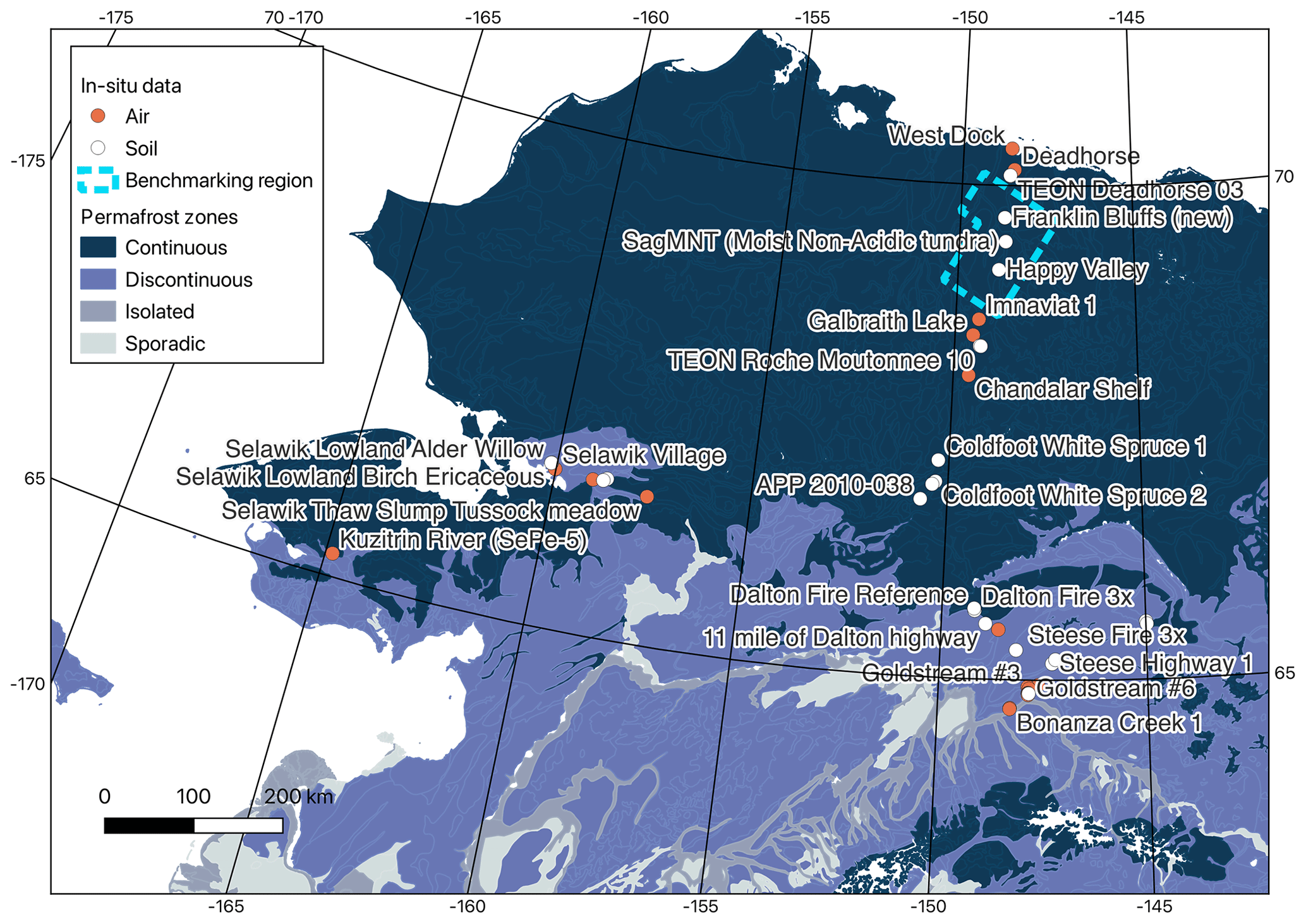
Figure 1 Location of in situ data sites with air (red) and soil (white) temperature for 2018 to 2020 (sources: Romanovsky et al., 2020, 2021, 2022). Background: permafrost zones from Jorgenson et al. (2008); shown with dark blue to light blue are continuous, discontinuous, sporadic, and isolated permafrost zones. The dashed outline indicates the region for benchmarking and fusion.

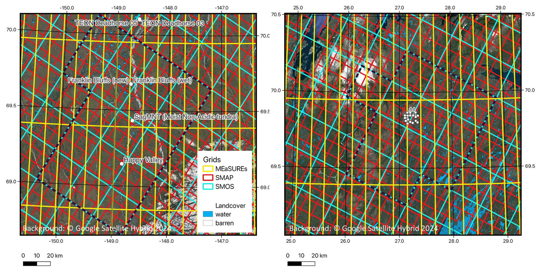
Figure 2 Examples of satellite product grids (see Table 1) for sites with in situ borehole data on the Alaska North Slope (left) and iButton data at Kaldoaivi, northern Finland (right). Background: Google Hybrid overlain by selected land cover classes relevant for masking (source: Bartsch et al., 2023d). In situ sites shown as filled white circles. Dashed black lines indicate the boundary of SMOS cell extent used for assessment and fusion. Grids of the passive microwave products (MEaSUREs, SMAP, and SMOS) differ in projection and extent. For details, see Table 1.

2.2 Global and Northern Hemisphere products

Three FT datasets based on relatively coarse-spatial-resolution PMW information are considered for benchmarking (Table 1). The currently listed FT Fundamental Climate Data Record (FCDR) in the catalog of CEOS (Committee on Earth Observation Satellites) Working Group on Climate is the MEaSUREs (Making Earth System Data Records for Use in Research Environments) Global Record of Daily Landscape Freeze/Thaw Status, Version 3 (Kim et al., 2014), which is associated with the ECV (Essential Climate Variable) soil moisture. It is based on various passive microwave missions (SMMR, SSM/I, and AMSR-E/AMSR2 (referred to as AMSR in the following)) and goes back to 1979. It is provided with 25 km gridding, separation of AM and PM, and >80 % mean annual spatial classification accuracy. FT information is supplied as a binary (either frozen or unfrozen). Vegetation-related use of the product is suggested apart from soil moisture masking (https://climatemonitoring.info/ecvinventory/, last access: 16 September 2024). An updated version (version 5), which is available through the National Snow and Ice Data Center (NSIDC; Kim et al., 2017, 2021), was used for this study. Version 5 is also considered for directly deriving land surface temperature for the production of climate records within the European Space Agency CCI LST project (Climate Change Initiative Land Surface Temperature, Dodd et al., 2021). The AMSR time series of the MEaSUREs dataset is available as a 6 km resolution record in addition to the 25 km record which includes time series from all sensors. The 6 km dataset covers the Northern Hemisphere and the Southern Hemisphere, currently spanning the period 2002–2021 (Kim et al., 2021). However, only the 25 km product (consistently with SSM/I) was used for this study. AM data were chosen where available since most available SAR data for the Alaskan benchmarking site (97 %) were acquired at AM times.

Table 1 Freeze–thaw datasets with Northern Hemisphere coverage considered for benchmarking with Sentinel-1 retrievals. V denotes vertical, H denotes horizontal, NPR denotes normalized polarization ratio, and SCV denotes single-channel vertical polarization.

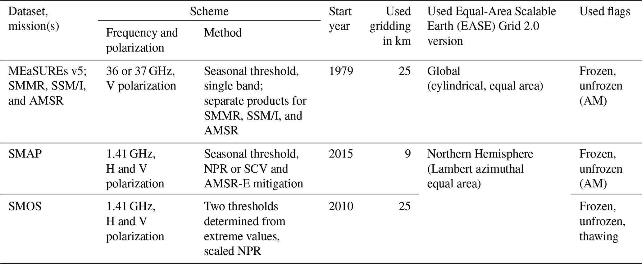
Further products exist from SMAP (2015 to present) and SMOS (2010 to present) and are available on an operational basis (Kraatz et al., 2018; Rautiainen et al., 2016). Both are L-band PMW missions and therefore provide information on the upper centimeters of the soil. The SMAP mission specifically targets freeze–thaw, complementing soil moisture, and requirements have been defined for the mission (Dunbar, 2018; Entekhabi et al., 2014). They have been phrased for the radar instrument (which is currently not in operation). The surface binary freeze–thaw state in the region north of 45° N latitude, which includes the boreal forest zone, was targeted with a classification accuracy of 80 % at 3 km spatial resolution and 2 d average intervals. A 2 d precision at the spatial scale of landscape variability (≈3 km) was originally targeted. The available SMAP PMW product considers four stages: frozen, thawed, transitional, and inverse transitional (Derksen et al., 2017). The two transitional categories refer to days with differences between AM and PM acquisitions. The SMAP product shows >70 % accuracy for the 36 km grid version according to Kraatz et al. (2018). Accuracies of 78 % and 90 % were determined for descending (AM) and ascending (PM) orbit observations, respectively, in relation to independent surface-air-temperature-based FT estimates from ∼5000 global weather stations (Kim et al., 2019). The SMOS mission FT product addresses three stages, namely thawed, partially frozen, and frozen, covering the Northern Hemisphere (daily, 25 km; Rautiainen et al., 2016).

The different sensors represent different frequencies (see Table 1), and different strategies were followed for the FT retrieval. The MEaSUREs algorithm is based on a seasonal-threshold approach. The threshold was derived annually on a grid-cell-wise basis (Kim et al., 2017) using an empirical relationship between brightness temperature and daily surface air temperature records from global model reanalysis. The SMMR-SSM/I-SSMIS record was developed by merging the Scanning Multichannel Microwave Radiometer (SMMR), Special Sensor Microwave Imager (SSM/I), and Special Sensor Microwave Imager/Sounder (SSMIS) 37 GHz frequency (vertical polarization) brightness temperature records (Kim et al., 2014). The AMSR records represent 36 GHz. The global 25 km datasets are provided as a cylindrical, equal-area projection, which translates to 10 km×62.5 km at the latitude of the benchmarking sites (Fig. 2).

SMAP FT state was determined using a seasonal-threshold approach (Derksen et al., 2017). A normalized polarization ratio (using V and H brightness temperature; 1.41 GHz) is assessed. Winter and summer references are derived from frozen and thawed soil conditions. These are calculated for each year and averaged over the entire SMAP period (according to the documentation of Xu et al., 2023). These values are used for the derivation of a threshold and a seasonal scale factor. In cases of low SCV (single-channel vertical polarization) correlation with physical surface temperature, SCV retrieval is used, and, in some cases, an AMSR-E mitigation scheme is applied (Xu et al., 2023). The dataset is provided in Lambert azimuthal equal-area projection and is available at 36 and 9 km (enhanced level 3) gridding. Only the latter was used.

Thaw and freeze references are also used in the case of SMOS FT retrieval (Rautiainen et al., 2016; Rautiainen and Holmberg, 2023). For FT state estimation, the normalized polarization ratio (NPR, 1.400–1.427 GHz) values are scaled using the reference NPR values from frozen and thawed soil conditions. All potential observations from the frozen and thawed soil conditions are collected from the winter and summer periods when reanalysis air temperature data indicated $<-\mathrm{3}$ and $>+\mathrm{3}$ °C, respectively. From these collected potential values, the 50 most extreme ones are stored, and their median is used as a reference value. These are pixel-wise values. Then two thresholds are used to differentiate between three FT states from the scaled NPR. The dataset is provided in Lambert azimuthal equal-area projection, with 25 km gridding.

Several active microwave products have been published previously but are limited temporally and spatially and are thus not considered for benchmarking. These include an experimental product from MetOp ASCAT (C-band scatterometer, 12.5 km gridding, Paulik et al., 2012), starting in 2007 and aimed at permafrost and flux applications (Naeimi et al., 2012). It is available at 12.5 km nominal resolution and considers three states: frozen, unfrozen, and melting. In addition, a C-band SAR product at 1 km was developed based on ENVISAT ASAR GM (Park et al., 2011) and was used to assess the ASCAT product (Bergstedt and Bartsch, 2017).

Benchmarking of the PMW datasets has been carried out over 17 SMOS grid cells (and overlapping SMAP and MEaSUREs cells) for Alaska and 12 cells for northern Finland (Fig. 2).

2.3 Temperature records

Temperature records from in situ observations include long-term measurement sites such as boreholes and automatic weather stations (AWSs), as well as short-term and spatially distributed observations using iButton data loggers. The latter network was established for validating surface conditions derived from C-band satellite data (for details, see Bergstedt et al., 2020b). These data have been used for inter-comparing Sentinel-1 with a coarser regional dataset based on MetOp ASCAT, covering the region of Kaldoaivi in northern Finland. This site is located within a palsa mire and represents a zone of sporadic permafrost. The temperature sensors have been distributed in the proximity of a permafrost borehole site. The majority of the iButtons are located outside of permafrost-affected landscape elements. The snow water equivalent (SWE) varies across the sites in winter, but at most sites, snow depth is sufficient for insulation, and temperatures remain close to 0 °C below the snowpack. The available record includes 24 sites, spanning a period of 2 years (August 2016 to August 2018). The iButton loggers were placed approximately 2–3 cm below the surface to avoid direct warming influence by the sun.

Records from boreholes and automatic weather stations (AWSs) across Alaska (Romanovsky et al., 2020, 2021, 2022), including the North Slope and representing continuous to discontinuous permafrost, have been used for calibration (Fig. 1). Data are available from 26 boreholes, with depths varying between 1–75 cm, and from 22 AWSs providing air temperature. A total of 3 years of data (2018 to 2020) have been used. ERA5 reanalysis air temperature data for the same time period were also used for the evaluation of the fused dataset to allow comparability with previous studies.

3 Methods

3.1 General workflow

First, the benchmarking dataset was created using Sentinel-1. The implementation of surface state classification, building on intermediate products of the wet-snow retrieval, as proposed in Nagler and Rott (2000), requires a threshold determination as a first step. For calibration, in situ data from Alaska limited to the upper few centimeters of the soil have been used. The target land cover type (as determined by the potential applications of an FT product) are soils. Water surfaces, bare areas, and glaciers therefore need to be masked with a dataset of similar spatial resolution (Bergstedt et al., 2020b). The circumpolar land cover units by Bartsch et al. (2024) fulfill this requirement and have therefore been used for masking.

Eventually, the frozen fraction is derived individually (spatial subsetting) from the masked data for each cell of the PMW FT products listed in Table 1. The resulting time series are used for the evaluation and the development of the fusion scheme. Fused records are assessed with the benchmark dataset in a similar way to the input records and the in situ records. The fused-record examples are combined with a dataset providing mid-winter thaw and refreeze of snow (Bartsch et al., 2023a), where such events occur, to facilitate the discussion.

3.2 Preprocessing of SAR data

The original wet- and dry-snow detection utilizes repeat pass dual-polarization Copernicus Sentinel-1 SAR data (acquired in IW swath mode) from different tracks. The method includes the generation of reference images, applying a statistical pixel-wise analysis of tens of co-registered repeat pass Sentinel-1 images (Nagler et al., 2016). To exploit the dual-polarization capabilities of Sentinel-1, the backscatter ratio of the snow-covered period and reference data are calculated separately for co- and cross-polarization and are then combined. The combination accounts for differences in the angular backscatter behavior of co- and cross-polarized backscatter data by applying the local incidence angle as a weighting factor. The result is a weighted ratio combination R_C (Nagler et al., 2016) based on the backscatter ratios of VV (R_VV) and VH (R_VH).

$$\begin{array}{}\text{(1)}& R_{\mathrm{C}}=W{R}_{\text{VH}}+(\mathrm{1}-W)R_{\text{VV}}\end{array}$$

The weight (W) varies with the local incidence angle (θ) by applying the following rule:

$$\begin{array}{}\text{(2)}& {\displaystyle }\begin{array}{rl}{\displaystyle }& {\displaystyle }\text{IF }(\mathit{\theta }<{\mathit{\theta }}_{\mathrm{1}})\to \mathit{\{}W=\mathrm{1.0}\mathit{\}},\\ {\displaystyle }& {\displaystyle }\text{IF }({\mathit{\theta }}_{\mathrm{1}}\le \mathit{\theta }\le {\mathit{\theta }}_{\mathrm{2}})\to \mathit{\{}W=k\left[\mathrm{1}+{\displaystyle \frac{({\mathit{\theta }}_{\mathrm{2}}-\mathit{\theta })}{({\mathit{\theta }}_{\mathrm{2}}-{\mathit{\theta }}_{\mathrm{1}})}}\right]\mathit{\}},\\ {\displaystyle }& {\displaystyle }\text{IF }(\mathit{\theta }>{\mathit{\theta }}_{\mathrm{2}})\to \mathit{\{}W=k\mathit{\}}.\end{array}\end{array}$$

For the datasets in this study, we use k=0.5, θ₁=20°, and θ₂=45° following Nagler et al. (2016). The SAR data have been sampled to 100 m×100 m.

More than 1900 scenes have been preprocessed in total over both regions. In situ locations in Alaska were covered by 52 to 179 scenes each. A total of 115 scenes have been used over Finland for comparison with in situ records. The time period covered for Finland corresponds with the in situ data availability (August 2016 to August 2018, with acquisitions every 12 d). Data processed for Alaska span 3 years, from 2018 to 2020 (with, on average, an acquisition every 9 d using overlapping orbits). This results in differing sampling intervals between the regions and lower sampling compared to the global FT records.

3.3 Freeze–thaw retrieval from SAR data and evaluation

The last step of the wet-snow retrieval scheme of Nagler et al. (2016) is the segmentation of wet-snow areas versus snow-free and dry-snow areas based on the R_C images (Nagler et al., 2016). This step was adjusted for the FT retrieval. Specifically, a suitable threshold Thr needed to be defined for the segmentation of frozen versus unfrozen soil.

The threshold determination followed the approach originally suggested for VV backscatter time series by Naeimi et al. (2012) (scatterometer) and adapted by Bergstedt et al. (2020b) (SAR). The threshold was defined based on a logistic function fit between backscatter and temperature data and the threshold Thr determined from the inflection point. This was based on reanalysis data in Naeimi et al. (2012). Bergstedt et al. (2020b) tested the calibration based on in situ air temperature over a limited number of sites and validated the results with in situ near-surface soil temperature data. Here, we also used in situ data for the air and soil but from a larger dataset and also for calibration. Air and soil temperature time series were compared to the R_C value of each corresponding 100 m×100 m SAR pixel. The inflection point of the fitted function was derived for both types, and the corresponding backscatter value was used as a threshold to distinguish between frozen (≤Thr) and unfrozen (>Thr) conditions. Here, we applied it to the combined VV and VH ratio values (R_C) as defined in Nagler et al. (2016). The logistic function was defined based on the processed R_C data on the Alaska North Slope. The fitting procedure included the consideration of the maximum value of R_C and the average for all values acquired under conditions below −5 °C. For the borehole records, the uppermost sensor below the ground was selected. Validation of the threshold approach was carried out based on the near-surface temperature observations available for northern Finland (Kaldoaivi). For this purpose, daily averages of 0 °C and lower were defined as frozen, and all values above 0 °C were defined as unfrozen.

A disadvantage of using backscatter intensity at C-VV is the temperature dependence under cold conditions (Naeimi et al., 2012; Bergstedt et al., 2020b; Bartsch et al., 2023b). The potential influence was therefore also investigated using the available in situ records. In addition to R_C, C-VV and C-VH backscatter intensity input values were compared with the temperature measurements for this purpose.

3.4 Subsetting global and fused dataset records for evaluation

The available global products represent varying grids. Therefore, the Sentinel-1 backscatter ratio analyses needed to be carried out over sufficiently large areas in the proximity of the in situ locations (overlap of grids, Fig. 2). The benchmarking extent was chosen considering both in situ data availability and the distance from the coast in order to limit potential quality issues in the PMW datasets. Both sites are labeled as high-quality areas in the MEaSUREs dataset. SMOS quality flags indicate, temporarily, up to 5 out of the 17 cells as being potentially affected by radio frequency interference (RFI) over northern Finland. No RFI issues are listed for the Alaskan sites. SMAP flags indicate retrieval with SCV (single-channel vertical polarization) due to a correlation of <5 % with temperature data and, in some cases, the use of AMSR or TB (brightness temperature) mitigation. The latter occurred only outside of the transition periods, in mid-summer and mid-winter (Fig. A1 in the Appendix). For Alaska, this includes mostly the end of December to the end of March and, in some cases, also July and August. For Finland, flagging occurred from July to September (where freeze-up starts in October).

Permanent snow- and ice-covered areas, water, and barren surfaces (bedrock) have been extracted from land cover for the masking of “none-soil” fractions in the SAR images. The none-soil fraction can be very large in permafrost environments. Figure 2 shows lakes and bare area as derived from a land cover map (Bartsch et al., 2023c). Both land cover types were excluded from the frozen-fraction calculations.

The frozen and unfrozen fractions were derived for each of the overlapping footprints of the PMW products (grid cells as shown in Fig. 2). The proportion of unmasked Sentinel-1 pixels classified as frozen has been determined for each acquisition. Basic statistics were derived for each global product separately (including for the presentation of results as violin plots).

3.5 Fusion: scheme and evaluation

Criteria for the preference of a certain dataset were eventually defined for a fusion scheme based on the benchmarking. The year is split into three phases for this purpose: DOY (day of year) 1–209, 210–300, and >300. In a first step, the datasets to be considered for a certain period were selected. In a second step, the conditions were defined (considering agreement between the datasets and/or the results of benchmarking). The combined dataset (referred to as the fusion dataset) was eventually also compared to the benchmark dataset derived from the Sentinel-1 frozen fraction. The fusion of the daily records was made on the basis of the SMOS grid (25 km). All comparisons of the fusion dataset were also made on the basis of the SMOS grid. The partially frozen flag was analyzed separately from the other flags (thawed and frozen).

Data from three borehole locations on the Alaska North Slope were used for the assessment of the unfrozen and frozen flags (temperature sensors at 5–7 cm depth) of the fusion product. In addition, ERA5 reanalysis data (air temperature) were investigated at the same sites (for locations, see Fig. 2). The frozen state retrieval from the soil and ERA5 air temperature data was based on the following daily mean temperature thresholds: values $<-\mathrm{1}$ °C are considered to be frozen, and values >1 °C are considered to be unfrozen, while values in between are classified as partial thaw.

Days with midwinter thaw and refreeze of the snowpack or wet snow were not part of the benchmarking but can potentially also be added using existing products. As an example, mid-winter thaw and refreeze, as available from the combination of MetOp ASCAT and SMOS (Bartsch et al., 2023b), have been added, and a flag value has been assigned. Such data are applicable for November to February (day of year 300 to 60).

4 Results

4.1 Temperature effect

The influence of temperature on C-VV backscatter as described in Bergstedt et al. (2020b) and Bartsch et al. (2023b) does not apply to VH (Fig. 3). Backscatter remains at a similar level for all temperatures below 0 °C at this polarization combination. Differences between the years due to changes in snow structure, as can occur, in particular, due to rain-on-snow events (Bartsch et al., 2023b), are also less pronounced at VH. The temperature influence is visible in the combined VV and VH ratio values (R_C increasing with decreasing temperature), inherited from VV, but the magnitude is lower than in the VV input data.

Figure 3 Sentinel-1 backscatter intensity at VV and VH (a) and combined ratios R_C (b) (92 acquisitions) versus daily sub-ground temperature (7 cm depth, 5 June 2018 to 27 December 2020) at Sagwon (SagMNT, Alaska). For location, see Fig. 1.

4.2 Sentinel-1 threshold determination and validation

The determined value of the inflection point from the logistic function fitting varies across sites (examples for comparison with soil temperature in Fig. 4). The spreads of the ratio values in winter and in summer are large, on the order of 1 to 2 dB, but they are largely distinct.

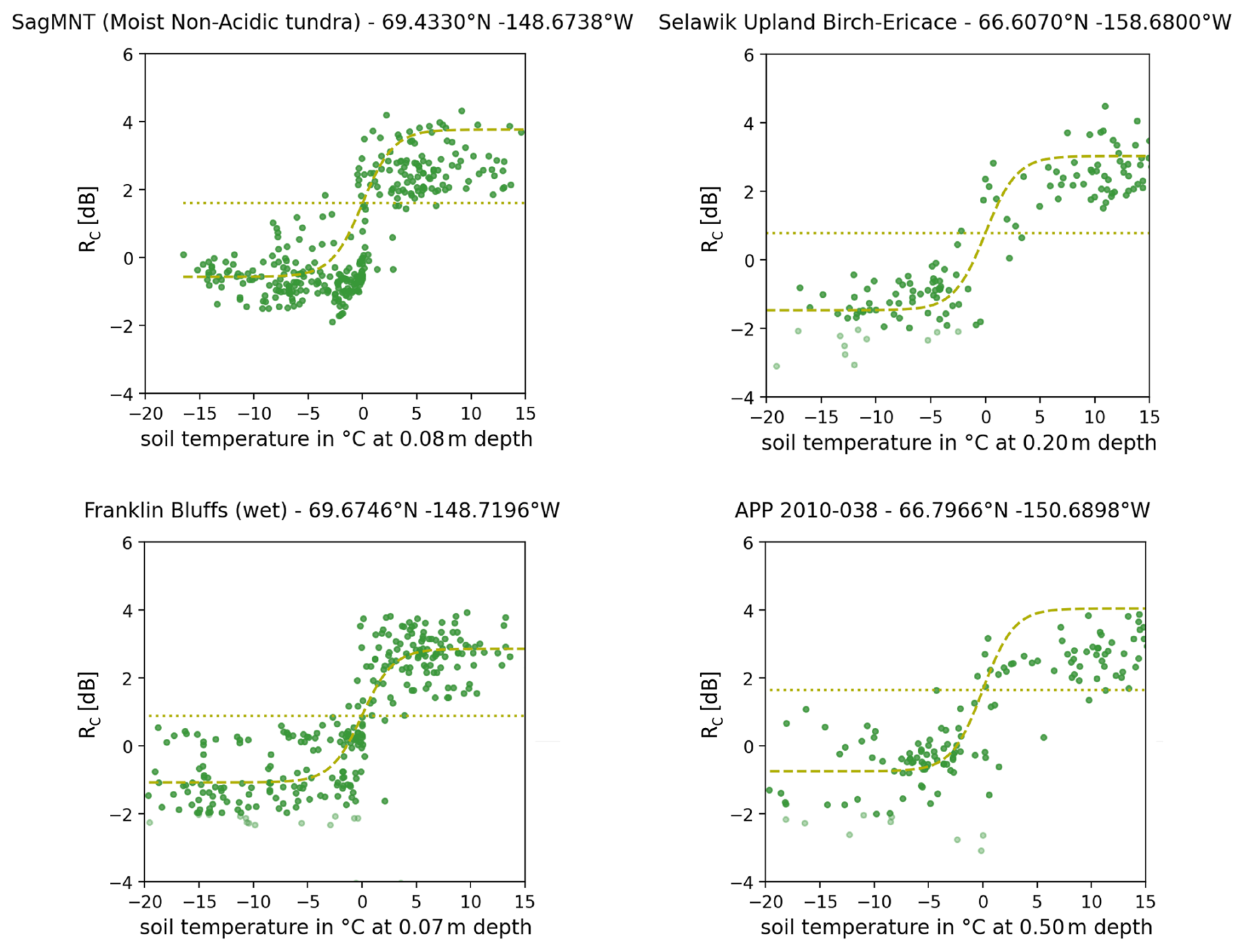
Figure 4 Examples for threshold determination at four borehole sites. Sentinel-1 combined polarization ratios (R_C) and in situ soil temperature are compared. Light green indicates R_C values below the wet- or dry-snow threshold (as defined in Nagler et al., 2016). The dashed line represents the fitted function. The dotted line represents determined inflection point. For location of sites, see Fig. 1.

Only minor differences are found between results using soil temperature and air temperature data (Fig. 5). The mean values of the inflection point differ by only 0.12 dB. The range is higher for air temperature. All values are higher than the suggested threshold for wet snow (−2 dB, Nagler et al., 2016). Most inflection point values even exceed it by more than 3 dB. A threshold of 1.34 dB based on the soil data (median) is suggested for regions with a soil layer that can contain water and/or ice (basic requirement for FT detection).

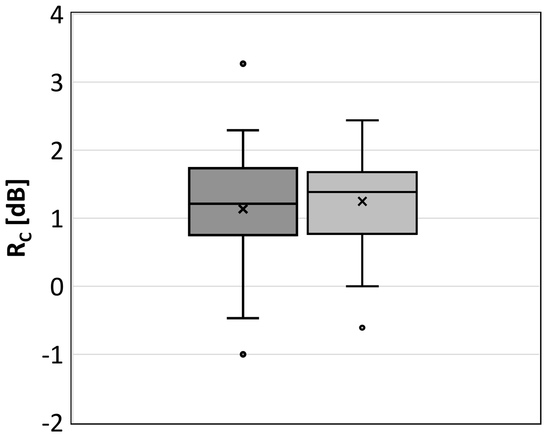
Figure 5 Sentinel-1 combined polarization ratio (R_C) statistics (boxplots) of inflection points of the logistical function fitted to temperature data following the threshold detection method of Naeimi et al. (2012) (air and soil temperature – 26 and 22 samples, respectively; in situ record overview in Fig. 1).

The applicability of the threshold could be confirmed using independent records by means of the in situ data from northern Finland (Kaldoaivi region; see Table 2). In total, more than 1800 samples of daily average temperature from 24 sites have been available for the Kaldoaivi region. A total of 93.2 % and 91.2 % (average 91.8 %) of all samples within the 2-year time period were correctly classified for the unfrozen and frozen conditions, respectively.

Table 2 In situ datasets used for calibration and validation of the benchmark dataset creation, as well as for the fusion assessment. AWS (automatic weather station) and borehole record sources: Romanovsky et al. (2020, 2021, 2022).

4.3 Freeze–thaw fraction within PMW grids

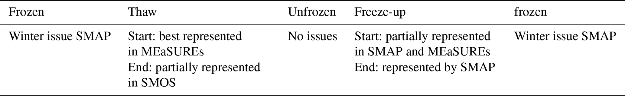
Only grid cells of the PMW datasets that are completely covered by the Sentinel-1 scenes have been cross-compared (Alaska: Fig. 6; Finland: Fig. 7). The shown results are limited to two periods, namely from April to June (from completely frozen to completely unfrozen) and from August to November (from completely unfrozen to completely frozen), in order to identify potential issues for the different transition types. Violin plots have been chosen to visualize the data distribution (of frozen fraction) for thawed and frozen conditions as defined in the products. For SMOS, the fraction was also analyzed for the thawing flag, which represents partially unfrozen conditions. Time series examples are provided for two distinct borehole locations, namely Happy Valley and Sagwon (Fig. 8). The frozen flags of each product were translated into values of 10 (unfrozen), 20 (partially frozen), and 30 (frozen) for comparability in these cases. Near-surface soil temperature and frozen fraction are shown together with the new flag values. In spring, the frozen fraction as detected by Sentinel-1 drops when the in situ temperature (1 cm depth) starts to rise above the late-winter level at Happy Valley. This drop does not coincide with the beginning of the thaw in the PMW cells. The start of the frozen-fraction increase does, however, agree with the drop below 0 °C in the 2020 example. This is similar for the second site (Sagwon, 8 cm depth, Fig. 8). Both borehole records show the so-called zero-curtain effect at freeze-up. Temperatures can remain at almost 0 °C for weeks to months due to latent heat, which maintains the temperatures (Outcalt et al., 1990). The frozen fraction is already at 100 % weeks before the ground temperature eventually lowers.

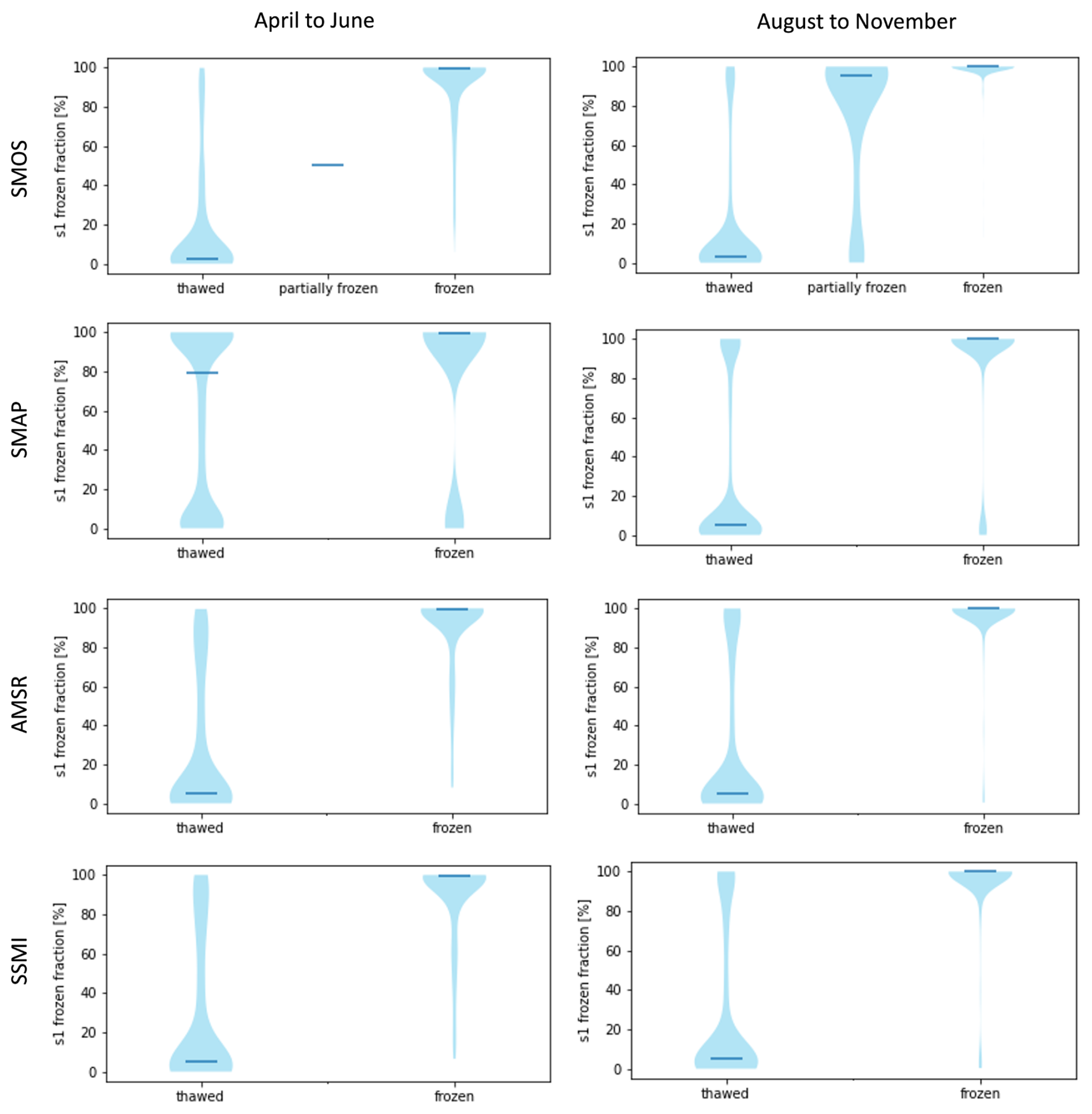
Figure 6 Sentinel-1 (s1)-derived frozen fraction for footprints of SMOS, SMAP, and MEaSUREs (AMSR and SSMI) freeze–thaw products. Sample period of 2017 to 2020 on the Alaska North Slope. Horizontal lines indicate average values. For analysis extent, see Fig. 2.

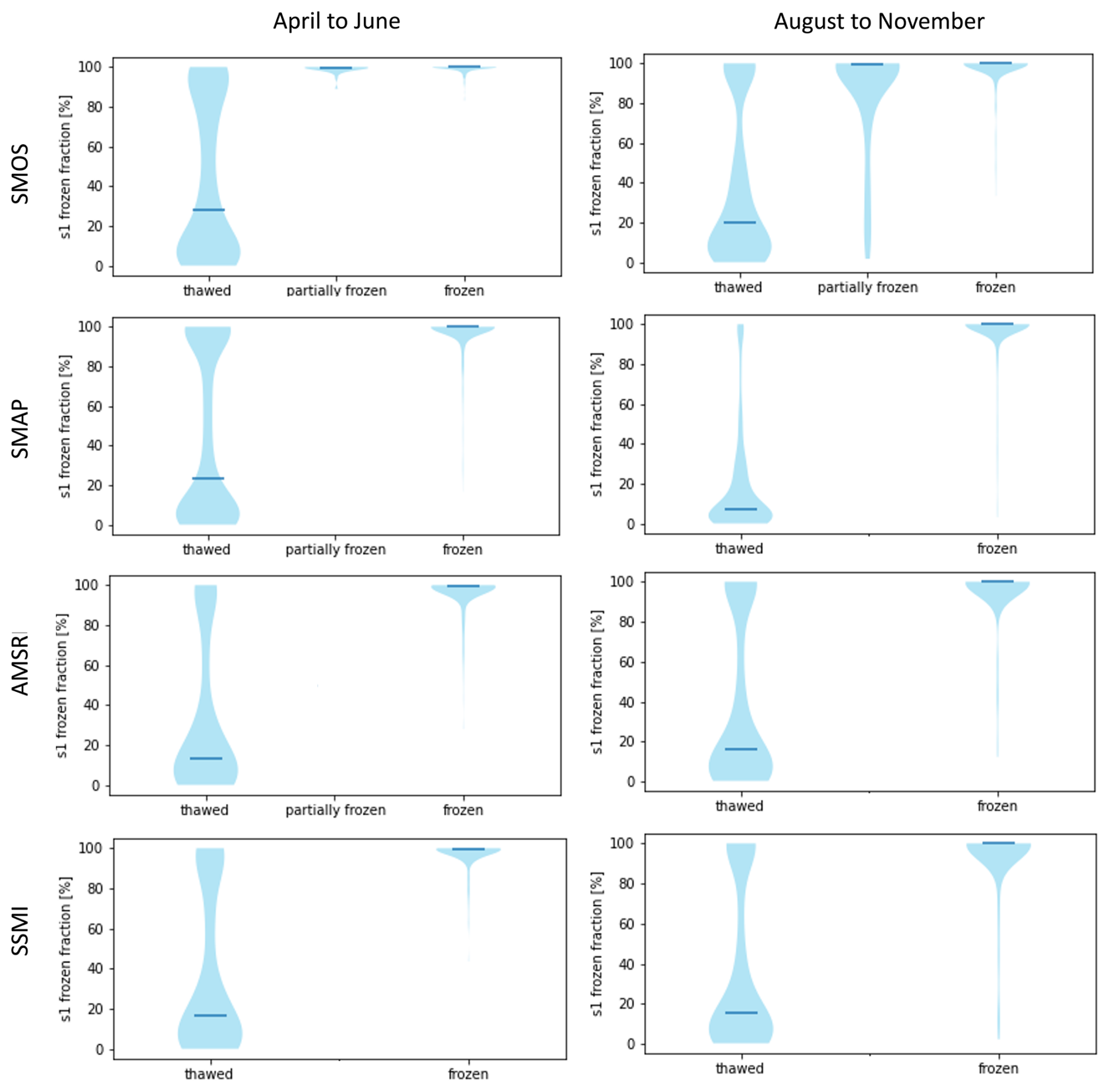
Figure 7 Sentinel-1 (s1)-derived frozen fraction for footprints of SMOS, SMAP, and MEaSUREs (AMSR and SSMI) freeze–thaw products. Sample period of 2018 to 2020 in Kaldoaivi, Northern Finland. Horizontal lines indicate average values. For analysis extent, see Fig. 2.

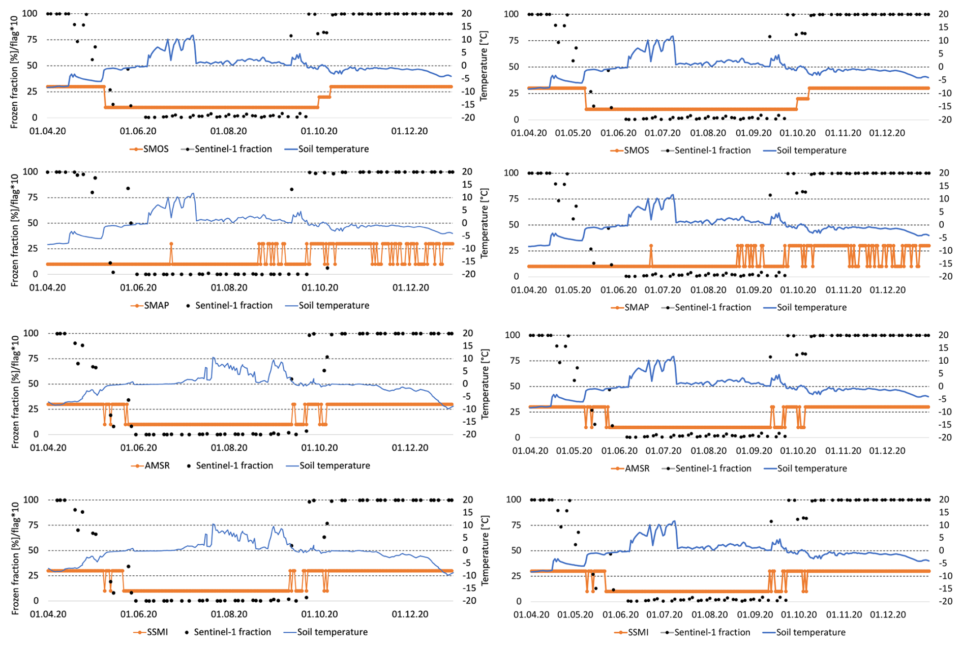
Figure 8 Time series for grid cells of passive microwave (PMW) freeze–thaw products (see Table 1) overlapping with the Happy Valley borehole location for 2020 (left) and the Sagwon (SagMNT) borehole location for 2019 (right). Near-surface soil temperature (1 and 8 cm, respectively), Sentinel-1 frozen fraction (differs between PMW datasets due to differing grids), and scaled freeze–thaw flags (10 – unfrozen, 20 – partially frozen, 30 – frozen, 0 – no data).

The fraction comparison clearly shows a frozen-state detection issue for SMAP during the winter on the Alaska North Slope (Fig. 6). A higher number of grid cells is defined as unfrozen than for the other datasets. This effect is more pronounced for April to June than for August to November. This leads to a premature thaw detection in spring. The timing of complete freeze-up is, however, generally captured when the flag switches from unfrozen to frozen, as can be demonstrated for the Happy Valley borehole location for 2020 (Fig. 8). The unfrozen flag is assigned to the SMAP grid cell from the beginning of the depicted time period, starting on 1 April 2020. The frozen fraction as determined by Sentinel-1 drops below 100 % towards the end of April and reaches 0 % in June. The unfrozen-flag issue at Happy Valley returns in mid-November. This happens only occasionally at the Sagwon site (Fig. 8). AMSR and SSMI flags switch from frozen to unfrozen by the end of May, when the Sentinel-1 frozen fraction is at almost 0 %. The partially frozen flag in SMOS only occurs here in autumn (coinciding with a frozen fraction of about 80 %); this can also be shown for a further borehole location for the autumn transition in 2019 (Sagwon, Fig. 8) and agrees with the fraction comparison results from the North Slope (Fig. 6).

SMOS captures the middle to the finalization of thaw on the North Slope well and is closer to the start of thaw for northern Finland (unfrozen flag includes a higher fraction of frozen conditions, Fig. 7). Freeze-up is detected with a delay. The majority of days with the partially thawed flag show almost complete freeze-up (spatially) in Sentinel-1. The MEaSUREs AMSR and SSMI products largely agree with each other (time series examples in Fig. 8). The spring switch occurs at the start to the middle of the thaw at the Happy Valley borehole location. The average frozen fraction with the unfrozen flag in spring is lower than for the other products.

The benchmarking results suggest the need for a fusion of all available products (Table 3). This allows a start of the time series in 2015 only (SMAP launch). The start and end of thaw can be represented back to 2010 (SMOS). The MEaSUREs records back to 1979 allow good detection of the start to the middle of the thaw.

Table 3 Summary of benchmarking results considering the target transition periods.

4.4 Suggested fusion scheme based on the benchmarking

SMOS and MEaSUREs (SSMI or AMSR) are recommended for consideration in all three time periods (Table 4). The performance of these products was shown to be similar for early winter; therefore, either of the products can be used. For late winter and during the thaw period, differentiation needs to be made in terms of whether the different products agree with each other or not. SMAP is recommended for consideration in the definition of the partially frozen flag during freeze-up, specifically when its flags disagree with the other products.

Table 4 Fusion scheme recommendation for the Northern Hemisphere. For product details, see Table 1. In the case of AM and PM data availability, only AM data are to be considered.

The PMW products were fused following the rules defined in Table 4. SMOS and MEaSUREs are recommended for consideration in all three time periods. The SMOS grid cell definition was used as a basis (see also Fig. 2). The previously introduced scheme for flag values (10 – unfrozen, 20 – partially frozen, 30 – frozen) was applied.

4.5 Assessment of fused records

Records were fused for the same grid cells as for the initial frozen-fraction comparison. The assessment procedure followed the same procedure in the first step. The frozen fraction from Sentinel-1 (SMOS grid) was compared by flag and separately for the thaw and freeze-up periods.

In addition, the partially frozen flag has been assessed over three selected borehole locations. The frozen fractions for days flagged in the SMOS product were compared to the fused dataset in order to evaluate the added value of MEaSUREs flags. The frozen and unfrozen flags of the fused product were evaluated considering soil temperature from boreholes at two sites. Results based on reanalysis air temperature data (ERA5) representing an average over a larger area are provided in addition.

4.5.1 Alaska North Slope

The combination of the different products specifically improves the determination of the partially frozen flag for the spring transition (Fig. 9). No day with partially frozen conditions was contained in the SMOS product from April to June between 2017 and 2020. This gap can be filled by fusion with the MEaSUREs datasets. The majority of grid cells were frozen for days indicated to be partially frozen in the SMOS product for August to November for the same years. The fraction distribution is inverted through the fusion with SMAO and MEaSUREs (Fig. 10). The average frozen fraction for days defined as partially frozen for SMOS is >90 % (Table 5). The Sentinel-1 frozen fraction on days with the partially frozen flag after fusion is reduced, on average, to values between 40 % and 46 % at the test sites in Alaska (taking spring and autumn into account; see Table 5). Frozen-fraction values are higher in spring than in autumn (Fig. 10). The occurrence of the partially frozen flag in spring increased through the fusion. For example, unfrozen conditions were identified in both MEaSUREs records at the North Slope site on the 24 May 2018 (Fig. 11). The SMOS scheme identified frozen conditions. Parts of the grid cells were frozen according to Sentinel-1. The fusion result was partially frozen.

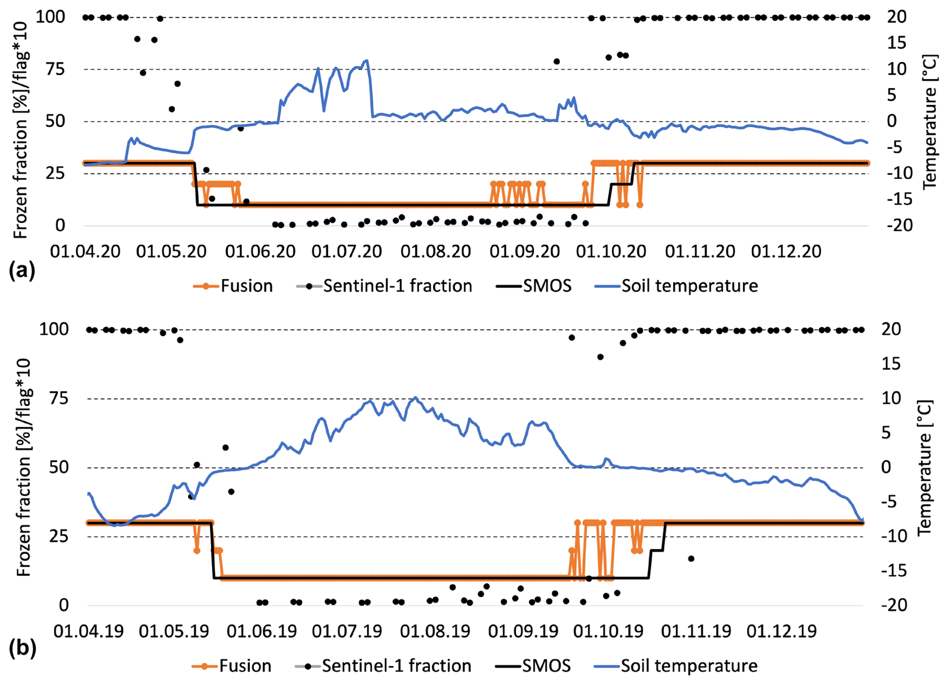
Figure 9 Time series example (spring and autumn) of the fused records for the SMOS grid point overlapping with the Happy Valley borehole location for 2020 (a) and the Sagwon borehole location for 2019 (b). Near-surface soil temperature, Sentinel-1 frozen fraction, and scaled freeze–thaw flags for SMOS and the fusion dataset (10 – unfrozen, 20 – partially frozen, 30 – frozen).

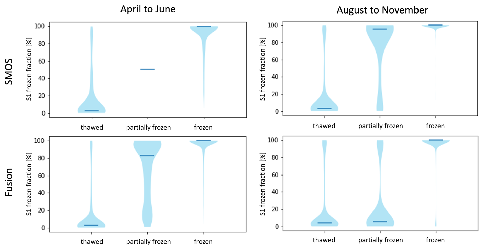
Figure 10 Sentinel-1 (s1)-derived frozen fraction for footprints of SMOS and the fusion dataset freeze–thaw state. Sample period of 2017 to 2020 on the Alaska North Slope. For analysis extent, see Fig. 2.

Table 5 Average Sentinel-1-derived frozen fraction (in %) for footprints of SMOS and the fusion dataset freeze–thaw state – days with partially frozen flag only. Sample period of 2017 to 2020 at three sites on the Alaska North Slope. For analysis extent, see Fig. 2. For product details, see Table 1.

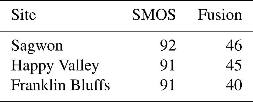
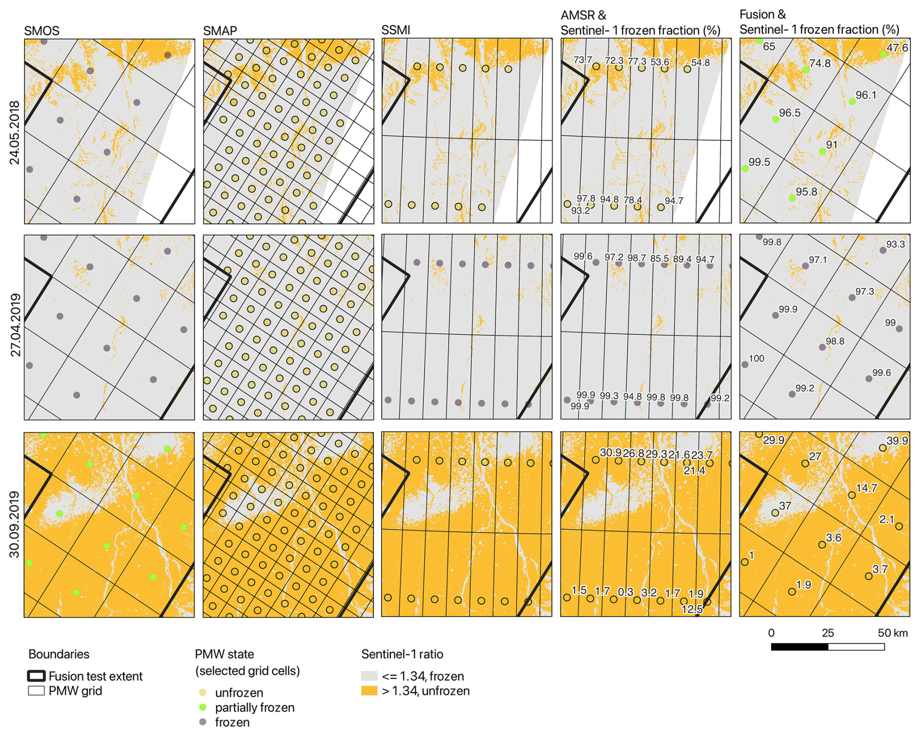
Figure 11 Example maps of Sentinel-1 and passive microwave (PMW) surface state, including fusion results for 24 May 2018, 27 April 2019, and 30 September 2019 (Alaska North Slope site). For location, see Fig. 2.

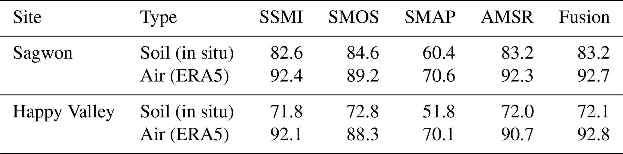
The agreement with near-surface soil temperature records and ERA5 air temperature for the frozen and unfrozen flags was similar for the MEaSUREs, SMOS, and fusion datasets. In general, values were higher for ERA5 (as data represent a grid average), and they were also similar between sites in this case (approximately 90 %, Table 6). The agreement with soil temperature differs between sites and was lower (70 %–80 %). Only SMAP showed a lower agreement for the sites on the Alaska North Slope, with values ranging between 51 % and 72 %.

Table 6 Agreement (in %) of freeze–thaw states derived from in situ soil temperature and ERA5 air temperature for all products and the fusion dataset result (gridded to SMOS) – days with unfrozen or frozen flag only. Sample period of 2017 to 2020 at two sites on the Alaska North Slope. For locations of sites, see Fig. 2. For product details, see Table 1.

4.5.2 Finland

Partially frozen conditions are also not captured in the SMOS product for April to June at the northern Finland site when only considering the in situ overlap period of 2016 to 2018 (Fig. 12) at a site located in a depression (at 337 m, with altitude ranging from 200 to more than 400 m in the surroundings). An extensive spring thaw period is identified with the fusion product in northern Finland, starting in early May 2017 (Fig. 13). In situ data from under the snowpack (thick enough to insulate the ground, with temperatures remaining at approximately 0 °C during the winter and as long as the snow remains) indicate that this period corresponds to snowmelt instead of near-surface soil thaw. The extended period of partially frozen conditions also disagrees with the frozen fraction from Sentinel-1 (Fig. 13). SMOS and AMSR show a high average frozen fraction with the thawed (unfrozen) flag over all analyzed grid cells (>20 %, Fig. 12). This also indicates a too-early thaw in this region. AMSR data were used for the fusion; however, this shifts some of these dates to partially frozen (Fig. 13). AMSR remained unfrozen until the start of the drop in the Sentinel-1 frozen fraction in 2017, while SMOS indicated unfrozen conditions from the beginning of May. This disagreement results in a partially frozen flag following the proposed fusion scheme. The end of this period coincided with the ERA5 temperature increase above 0 °C. The actual end of thaw for the entire grid cell was, however, 1 month later in early July.

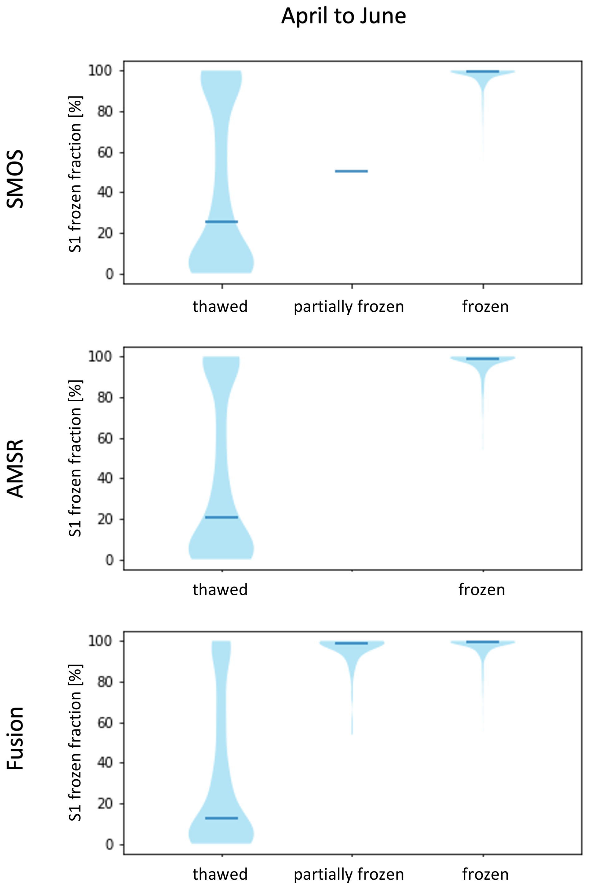
Figure 12 Sentinel-1-derived frozen fraction for the fusion dataset freeze–thaw state (footprints according to SMOS product) in Kaldoaivi, northern Finland. Sample period of 2016 to 2018. For analysis area and extent, see Fig. 2.

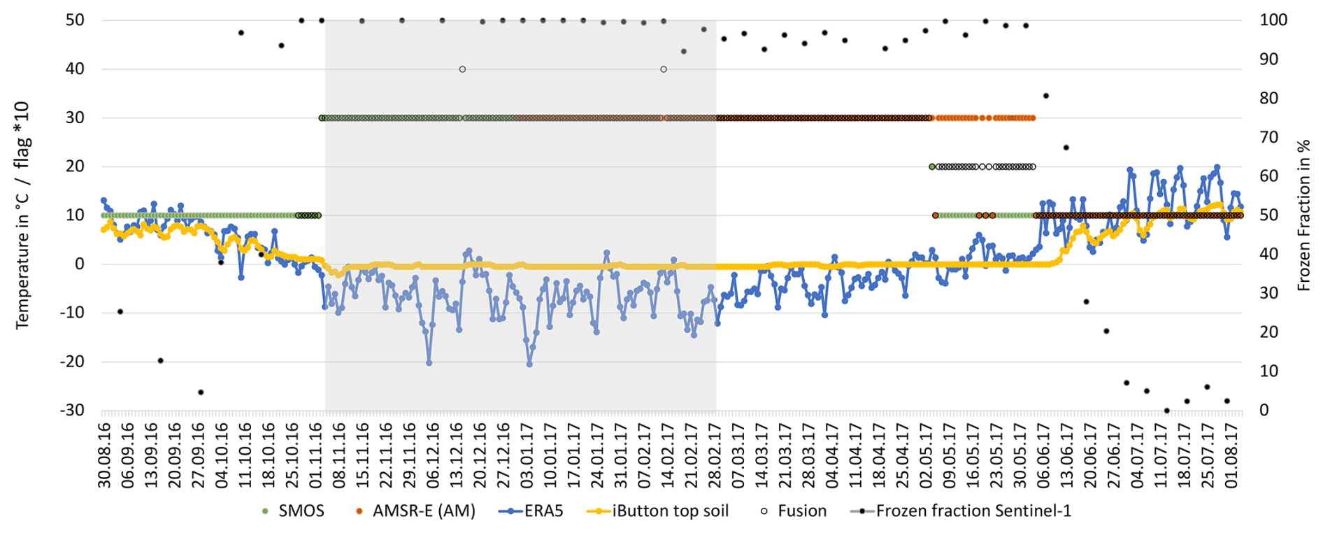
Figure 13 Comparison for SMOS grid point overlapping with the northern Finland site for autumn 2016 and spring 2017 (altitude range 200–400 m). Near-surface soil temperature (iButton location A4 at 337 m altitude, Bergstedt et al., 2020b); ERA5 temperature; Sentinel-1 frozen fraction; scaled freeze–thaw flags for SMOS, AMSR, and fusion dataset (10 – unfrozen, 20 – partially frozen, 30 – frozen, 40 – mid-winter thaw and refreeze). The shaded area indicates the analysis period for mid-winter thaw and refreeze (source: Bartsch et al., 2023b).

The fusion result example in Fig. 13 also includes the occurrence of mid-winter FT (source: Bartsch et al., 2023b). The detected events (15 December 2016, 13 February 2017) correspond to periods with ERA5 temperatures above 0 °C. All analyzed PMW products indicate frozen conditions for those dates.

Frozen-fraction values on partially frozen days are high in spring and autumn, which differs from the Alaska North Slope results. However, they are lower than in the SMOS product. The fusion reduces the high-frozen-fraction detection for the thawed state for both spring and autumn.

5 Discussion

5.1 Benchmark dataset

The use of combined ratios of backscatter intensity using VV and VH polarization, as previously suggested for wet-snow detection, provides a means of reducing the incidence angle effects, but the impact of temperature variations on backscatter intensity at VV during frozen conditions remains (Fig. 3). The combined ratio R_C also shows this linkage. The potential influence of temperature on FT retrieval at C-VV has been previously discussed (Naeimi et al., 2012; Bergstedt et al., 2018; Bartsch et al., 2023a). Our results demonstrate that this is specific for VV but not present in VH (Fig. 3). The retrieval based on VH alone would, however, require an appropriate approach regarding the influence of the incidence angle, such as the normalization of σ₀ (Widhalm et al., 2018) or the retrieval of γ₀ (Small, 2011). An implementation based on VH would also require a location-specific threshold determination (instead of a global threshold), which is not feasible for the purposes of this study and for potential regional applications of the FT detection approach.

The combined-ratio approach does, nevertheless, provide good-quality results. The overall agreement with in situ data of 92 % at the site in northern Finland is similar to the previously reported accuracy of 94 % using the location (pixel)-specific threshold determination approach (Bergstedt et al., 2020b). The validation was carried out over a different region (northern Finland) than the calibration (Alaska North Slope), confirming the transferability of the method. The performance is also similar to a CNN (convolutional neural network) approach using both polarization bands (88 %, with calibration and validation over the same region in NE Canada; Chen et al., 2024).

We tested the combined-ratio approach over tundra only. It can be expected that the performance would be lower over forested regions as it relies on the use of VH. A method using VV only, such as that suggested by Cohen et al. (2021), might perform better for forested areas.

5.2 Global and Northern Hemisphere product benchmarking

The SMOS–Sentinel-1 comparison results agree with findings of Cohen et al. (2021). Offsets in the FT timing compared to in situ measurements were described and attributed to the ability of the L band to represent larger soil depths. SMAP, which is also based on the L band, does, however, represent the end of the autumn freeze-up period well. The AMSR and SSMI frozen flags also indicate a later freeze-up in some cases (multiple switching from frozen or unfroze; see Fig. 8), although a much smaller wavelength is used.

Differences in wavelength and/or frequency (see Table 1) are expected to contribute to the deviations between the results in addition to differences in the FT classification method, although all of this depends on thresholding. The MEaSUREs scheme relies on the use of one polarization only, with, at the same time, a comparably small wavelength and high frequency. Both SMOS and SMAP FT products are based on the use of the NPR, which uses two polarizations but at a comparably large wavelength and small frequency. Whereas a single threshold is used to separate thawed from frozen conditions for SMAP, two thresholds are used to derive partially frozen conditions in the case of SMOS. The thawed fraction derived from Sentinel-1 is, however, rather low in most cases of the partially frozen condition (Table 5). This applies specifically for the spring transition (Fig. 7). Once SMOS has indicated a frozen soil condition, the mid-winter values are forced to remain frozen under cold air temperature conditions (Rautiainen et al., 2016; Rautiainen and Holmberg, 2023), which may contribute to the better agreement with the benchmarking dataset during this period than for SMAP. Both SMOS and SMAP can be affected by RFI. The SMOS quality flags indicate a potential impact for the Finland site but not for northern Alaska. Thus, the different results for Alaska, as shown in the example of Fig. 11, may originate from the threshold definitions and the consideration of a single channel (V) under certain conditions in the case of SMAP. The latter was developed for low latitudes according to the product documentation (Xu et al., 2023).

SSMI and AMSR records showed very similar performances (e.g., Table 6). The AMSR time series, as part of the MEaSUREs dataset, is also available at 6 km nominal resolution. The use of this version might be of benefit, replacing both the 25 km AMSR and SSMI records. Further analyses would, however, be required for the quantification of the added value of the improved spatial resolution.

The comparison with the Sentinel-1 frozen fraction and in situ data with the seasonal freeze–thaw prototypes indicates an improvement through the fusion of the different products. However, a range of issues, which differ between the evaluation sites (continuous permafrost over Alaska versus sporadic permafrost for northern Finland), remain. Neither the actual end of thaw in spring nor the start of freeze-up in autumn can be captured. These issues cannot be solved based on the existing passive-microwave-based CDRs.

The frozen fraction derived from Sentinel-1 only applies to areas without open water and barren surfaces. Therefore, the deviation of the PMW products could also be analyzed with respect to the open-water fraction, as has previously been investigated for active microwave freeze–thaw (Bergstedt et al., 2020a), in order to provide more insight into product issues. An offset in freeze–thaw timing can be expected in relation to lake ice thaw and formation.

Previous analyses of C-band scatterometers indicated the applicability of active microwave data for FT retrieval in high-latitude regions (e.g., Naeimi et al., 2012). Specifically, the fusion of SAR and scatterometers is promising for the characterization of the transition period (actual determination of the start and end; Bergstedt et al., 2020b). The new SAR-based method which has been developed in our study enables operational retrieval of surface state from sensors such as Sentinel-1 and theoretically allows us to meet the requirements for a multipurpose FT product if sufficient acquisitions (daily) are available. In addition to soil FT, wet-snow detection could also be addressed as it is based on the same preprocessing scheme. The availability of Sentinel-1 data is, however, constrained, and the polarization differs across the Arctic. The required data are unavailable for Greenland and the Canadian High Arctic. In the remaining regions, repeat intervals are not dense enough (daily required). However, Bergstedt et al. (2020b) demonstrated the use of historic (1-year) Sentinel-1 data for the calibration of a freeze–thaw fraction derived from MetOp ASCAT. FT monitoring considering fraction could therefore be implemented in regions with VV and/or VH availability. Retrieval with HH (horizontally sent and received) and/or HV (horizontally sent and vertically received) remains to be tested. An implementation based on MetOp ASCAT would allow the production of a CDR going back to 2012 (MetOp-A and MetOp-B availability).

More advanced FT algorithms using dielectric models to represent non-linear behavior in highly organic soils common in the Arctic may be able to detect changes in the amount of unfrozen liquid water remaining in soil under sub-zero temperatures rather than relying on simple binary FT thresholds (e.g., Wang et al., 2024). Another advanced method employed by Holmberg et al. (2024) shows potential for directly retrieving continuous soil permittivity data over cold regions, as has currently been demonstrated over a test site.

The current benchmarking exercise was limited to AM data in the case of MEaSUREs and SMAP due to the availability of Sentinel-1 data at the selected sites during this period. Diurnal thaw and refreeze are, however, common (e.g., Bartsch et al., 2007; Böttcher et al., 2018) during transition periods. The added value of PM data should be addressed in future studies considering other sites or further relevant SAR missions. The future L-band mission NISAR (Das et al., 2021; Rosen and Kumar, 2021) can be expected to be of high value for such benchmarking as it represents a similar frequency as that used for SMOS and SMAP, and a comparably high temporal sampling will be available. Our analysis is limited to non-forested areas due to the use of C-band SAR. L-band SAR provides the possibility to extend research into forests.

5.3 Global and Northern Hemisphere product utility

Current FT products aim for the identification of an average surface state condition within a footprint (e.g., Kim et al., 2014, using SSMI; Naeimi et al., 2012, using ASCAT; Derksen et al., 2017, using SMAP and Rautiainen et al., 2016, using SMOS), but specific applications, including permafrost, soil moisture, and greenhouse gas fluxes, require information on the start of thaw and/or freeze-up and the completion of thaw and/or freeze-up (Tables B1–B3, Bartsch et al., 2022).

5.3.1 Permafrost

The observation that the unfrozen period (complete thaw of grid cell) in high-latitude, relatively cold regions is longer in the case of SSMI than what is suggested by the benchmarking data (Fig. 8) agrees with findings of Kroisleitner et al. (2018). The unfrozen period was also found to be longer than for an experimental product based on MetOp ASCAT. This impedes the applicability for permafrost-related applications, such as the estimation of potential mean annual ground temperature. The impact on the capability to monitor long-term trends in frozen-period length (as suggested by Park et al., 2016a) remains to be investigated.

Kouki et al. (2019) also compared and evaluated datasets for the start of spring thaw. SSMI and SMMR switches from frozen to thawed were shown to correspond to the start of the increase in temperatures to above 0 °C, which agrees with the Sentinel-1 fraction and in situ borehole comparisons on the Alaska North Slope (Fig. 8). Results from northern Finland also indicate that the frozen–thaw switch (start of decrease in frozen fraction) coincides with increasing air temperatures but not with upper-soil temperatures (Fig. 13). Snow is still present on the ground at this time, as indicated through the temperature measurements (remaining stable close to 0 °C) and in situ measurements of snow depth in March 2018 (44 to 86 cm; Bergstedt and Bartsch, 2020).

A combination of MEaSUREs (SSMI and AMSR) and/or SMOS with SMAP (excluding the winter period) may fulfill the requirements for a freeze–thaw flag being used as proxy for potential permafrost occurrence. Threshold requirements (Table B1) could at least be partially met. Diurnal variations may need to be considered with respect to acquisition timing. Freeze–thaw cycles on a daily basis have been shown to be common during the spring period in the context of wet-snow detection (e.g., Bartsch et al., 2007). This pattern may extend into the snow-free period.

Ground temperatures can also be affected by the melting of snow in mid-winter (Westermann et al., 2011). Figure 13 provides an example of an existing microwave remote-sensing-based product and the co-occurrence of air temperature increases. As near-surface soil temperatures were already at 0 °C in this zone, with only sporadic permafrost, a temperature response was not detected. Previous studies, including that of Westermann et al. (2011), have, however, shown increases in colder regions. A combined product is therefore expected to be of benefit for permafrost applications.

5.3.2 Masking of soil moisture products

With the currently available FT products, target requirements for soil moisture (completely unfrozen determination; see Table B2) cannot be met for the transition periods. A partial solution provides the combination of SMOS and MEaSUREs for spring thaw. The combination improved the partially frozen flag of SMOS on the Alaska North Slope (Table 5). A precise determination of the start of freeze-up in autumn based on the existing products is currently not possible.

The results of Bergstedt et al. (2020b) indicate that MetOp ASCAT backscatter, in combination with Sentinel-1 frozen-fraction statistics, allows us to derive the start and end of the thaw and freeze transition. A calibration would, however, require the processing of Sentinel-1 for at least 1 year for each ASCAT footprint to be processed. The frozen fraction could be used similarly in the combination with the MEaSUREs and SMOS data for the spring period and for defining the start of freeze-up, which is not represented yet.

5.3.3 Vegetation and carbon flux applications

The combination of MEaSUREs, SMOS, and SMAP is expected to partially fulfill threshold requirements for the classification (Table B3) as the start and end of the transition periods are of relevance in this case. To fulfill the target requirements, the start of freeze-up would also be needed. The consideration of Sentinel-1-facilitated frozen-fraction retrieval would be of benefit. AM and PM information would eventually be required, in addition to an indication of the presence of melting snow, in order to monitor diurnal variations, which are of relevance for fluxes.

6 Conclusions

The joint use of VV and VH available from Sentinel-1 acquisitions has been shown to be applicable to FT retrievals in high latitudes. This allows for regional-scale analyses at a comparably high spatial resolution as a global threshold can be defined. The creation of a freeze–thaw benchmarking dataset requires sufficient temporal sampling at the same time. Both spatial coverage and temporal sampling are major constraints, but implementation based on Sentinel-1A and B is possible for some regions in the Arctic, including Alaska and northern Scandinavia. The resulting benchmarking dataset provides a means to address issues in coarse-resolution satellite products based on PMW data across the Arctic, although representing a different frequency. Current quality assessment with in situ data is limited due to the scarce availability of ground stations and their limited representativeness because of high landscape heterogeneity.

The thresholding and further parameterization applied to the two L-band records, SMAP and SMOS, result in substantial differences across all seasons between the products despite similar inputs. This might be specific to tundra environments. Further investigations are needed to identify actual error sources and to revise the fusion scheme for the identification of partially frozen conditions.

For global and Northern Hemisphere applications, coarser-resolution datasets such as the tested passive-microwave-based datasets need to be used at this stage. Improvements to the existing regional to global datasets are, however, needed. The transition periods are not well captured, even when a partially frozen flag is considered, as in the case of SMOS. Such a flag should be (1) included in any future coarse-spatial-resolution FT products and (2) improved upon in terms of precision in order to meet various user requirements. A fusion with SAR retrievals may allow us to overcome various error sources, specifically seasonally changing water surfaces, which are an issue due to the coarse spatial resolution of PMW observations. The utility of FT datasets could be further enhanced by means of combination with wet-snow products from direct observations or indirectly via snow structure changes resulting from refreezing snow.

A fusion of the existing products can only partially enhance the accuracy. The Sentinel-1-derived benchmark dataset provides a means for improving existing retrieval schemes and for the development of new products that rely on comparisons with in situ point or modeled and coarser-resolution reanalysis data. Comparison to in situ records also needs to consider soil temperature measurements in order to evaluate the role of snow.

Appendix A: SMAP data quality example

Figure A1 Examples of the SMAP quality flag for use of AMSR-E or brightness temperature mitigation (Xu et al., 2023) in 2021 (percentage per month).

Appendix B: User requirement summary from Bartsch et al. (2022)

Table B1 Requirements for an FT climate data record for permafrost monitoring in lowland areas in line with Permafrost_cci (Bartsch et al., 2023d).

Table B2 Requirements for an FT climate data record for the masking of soil moisture (National Research Council, 2014; Dunbar, 2018; Entekhabi et al., 2014; Trofaier et al., 2017).

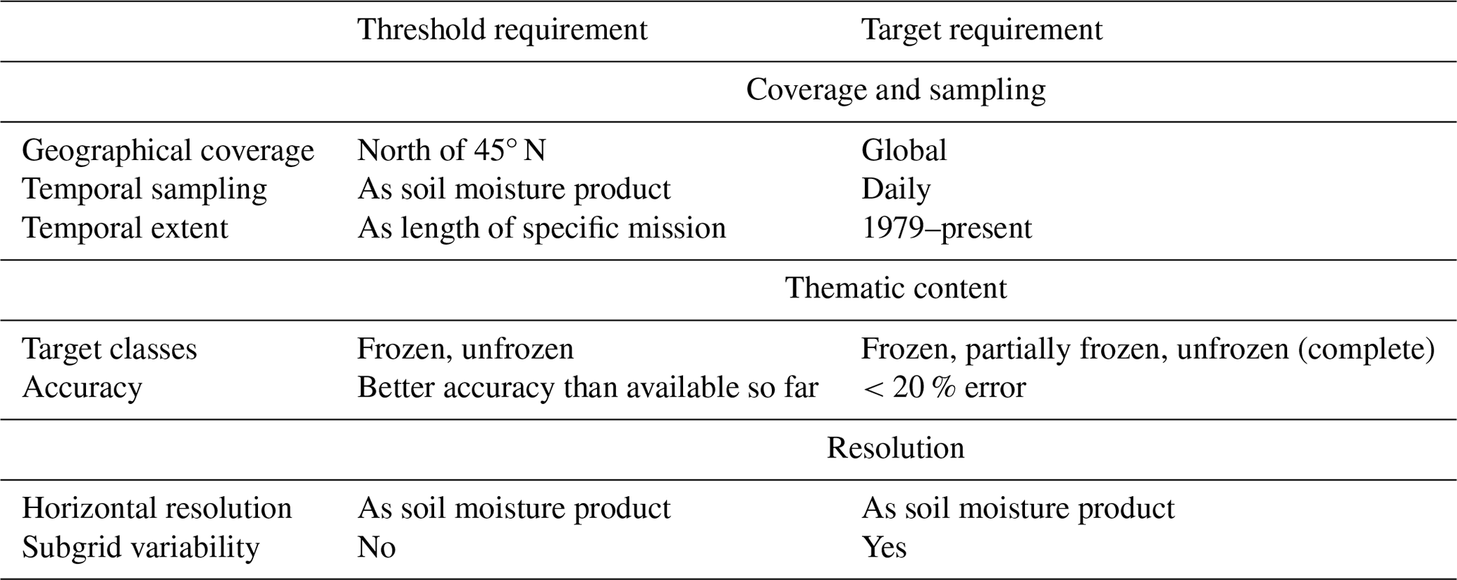
Table B3 Requirements for an FT climate data record for vegetation and carbon flux applications (Böttcher et al., 2018; Bartsch et al., 2007; Aalto et al., 2020).