UAV LiDAR surveys and machine learning improve snow depth and water equivalent estimates in boreal landscapes

Climate change is rapidly altering snow conditions worldwide, and northern regions are experiencing particularly significant impacts. As these regions are experiencing faster warming than the global average, understanding snow distribution and its properties at both global and local scales is critical for effective water resource management and environmental protection. While satellite data and point measurements provide valuable information for snow research and models, they are often insufficient for capturing local-scale variability. To address this gap, we integrated UAV LiDAR with daily reference measurements, snow course measurements, and a machine learning (ML) approach. Using ML clustering, we generated high-resolution (1 m) snow depth and snow water equivalent (SWE) maps for two study areas in northern Finland. Data were collected through four different field campaigns during the 2023–2024 winter season. The results indicate that snow distribution in the study areas can be classified into three categories based on land cover: forested areas, transition zones with bushes, and open areas (namely peatlands), each showing different snow accumulation and ablation dynamics. Cluster-based modelled SWE values for the snow courses gave good overall accuracy, with RMSE values of 31–36 mm. Compared to snow course measurements, the cluster-based model approach enhances the spatial and temporal coverage of continuous SWE estimates, offering valuable insights into local snow patterns at the different sites. Our study highlights the influence of forests and forest gaps on snow accumulation and melt processes, emphasizing their role in shaping snow distribution patterns across different landscape types in the Arctic boreal zone. The results improve boreal snow monitoring and water resource management, offer new tools and high-resolution spatiotemporal data for local stakeholders working with hydrological forecasting and climate adaptation, and support satellite-based observations.

1 Introduction

Snow is an important part of the hydrological cycle and is highly relevant to societies and ecosystems, especially in high latitudes and mountainous regions. Snow cover, timing, and distribution directly influence the climate energy budget through snow albedo (Callaghan et al., 2011; Li et al., 2018); ecosystems and habitats, including species and vegetation distribution (Thiebault and Young, 2020); and biogeochemical processes in soils and seasonal ground frost (Ala-Aho et al., 2021; Croghan et al., 2023; Jan and Painter, 2020). Additionally, snow resources have a major impact on catchment, river, and groundwater budgets and seasonal distribution (Meriö et al., 2019). Snow-covered areas are decreasing as global temperatures rise, leading to a consistent decline in snow water equivalent (SWE) (Colombo et al., 2022; Faquseh and Grossi, 2024; Kunkel et al., 2016; Räisänen, 2023; Zhang and Ma, 2018). A recent study by Gottlieb and Mankin (2024) shows how March SWE has decreased in half of the Northern Hemisphere river basins over the past 40 years, with the highest decreases in the southwestern USA and western, central, and northern Europe. The timing and amount of snowmelt, along with SWE in the melting period, are crucial for local water balance and flood monitoring and regulation (Bavay et al., 2013; Callaghan et al., 2011; Wang et al., 2016). Changes in snow conditions and rising temperatures are causing earlier flood peaks in snowmelt-dominated catchments, with a decline in streamflow later in the year (Berghuijs and Hale, 2025; Engelhardt et al., 2014; Matti et al., 2017). Snowmelt significantly influences near-surface hydrological effects (Muhic et al., 2023) and soil moisture in these regions (Okkonen et al., 2017).

Snow models are an important part of water resource planning and prediction. These models provide estimations of snow-related hydrological parameters for areas and times where ground observations are not available and can be used for creating various scenarios. However, for the accurate prediction of snow water resources, snow models require high-resolution data as inputs and for testing and validation. Satellite-based remote sensing is still a rather coarse tool and has limited accuracy with canopy cover (Muhuri et al., 2021; Rittger et al., 2020). For example, currently, the accuracy and spatiotemporal availability of SWE from microwave satellite missions are not sufficient for local-scale water resource management planning (Tsang et al., 2022). Gaffey and Bhardwaj (2020) conclude that as only a few satellite sensors provide the resolution required to capture local variability with multispectral or infrared data, together with limited revisiting times, the usage of satellite products in snow research is still limited. Thus, ground-based manual measurements, which are then fed into operational models, are still conducted. The national snow course measurement network – a manual snow depth and density measurement protocol – provides important data for models and serves as a long-term historical dataset; however, gathering data is time-consuming, the accuracy varies (Beaudoin-Galaise and Jutras, 2022; Kuusisto, 1984; Mustonen, 1965), and the temporal resolution is weeks to 1 month. Thus, it is not ideal for capturing the snow dynamics of individual events or important hydrological variables such as peak snow depth or melt-out dates (Malek et al., 2020).

To bridge the knowledge and technical gap between remotely sensed and ground observations, uncrewed aerial vehicles (UAVs) have been proven to be efficient in snow depth and SWE estimations, providing decent cost efficiency and accuracy (Adams et al., 2018; Niedzielski et al., 2018; Rauhala et al., 2023). Like satellite platforms, UAV systems can carry both optical and radar-based sensors and provide high-resolution spatial information. Photogrammetry, including multispectral and stereo-imagery, can result in centimetre-scale accuracy in snow depth mapping over a catchment scale and is relatively low cost compared to radars like ground-penetrating radar (GPR) and light detection and ranging (LiDAR) (Maier et al., 2022; Nolan et al., 2015; Rauhala et al., 2023). Combining snow depth data from LiDAR and spectrometer sensors has also been used to model snow density on a weekly basis at the Airborne Snow Observatory (ASO) (Painter et al., 2016). Yet, photogrammetry-based products, like structure-from-motion (SfM), require suitable light conditions and heterogeneous snow surfaces and are limited in penetrating dense vegetation cover. Thus, the decision between cost-effectiveness and accuracy is dependent on the site characteristics (Rauhala et al., 2023; Rogers et al., 2020). Recently, LiDAR sensors have become more affordable, compact, and lightweight. Technical advancements, such as improved inertial measurement units (IMUs) and global navigation satellite systems (GNSSs), have enhanced their accuracy and performance, making LiDAR more cost-effective and competitive compared to UAV photogrammetry (Bhardwaj et al., 2016; Rogers et al., 2020). UAV LiDAR technology potentially offers high accuracy over large spatial areas and allows catchment-scale mapping even under canopy cover, unaffected by overcast conditions or shadows (Dharmadasa et al., 2022; Harder et al., 2020; Jacobs et al., 2021; Mazzotti et al., 2019). LiDAR-based snow depth data, when combined with models or density assumptions, can also be used to estimate the spatial distribution of SWE on a landscape scale, with decent cost-effectiveness (Broxton et al., 2019; Geissler et al., 2023).

Snow conditions are mostly controlled by temperature and precipitation (Mudryk et al., 2020; Mudryk et al., 2017), and changes in global and local climate trends impact snow cover differently across regions. However, local snow accumulation is dependent on on-site characteristics, such as topography, vegetation, weather, and wind patterns (Currier and Lundquist, 2018; Mazzotti et al., 2019, 2023). Forest structure significantly affects snow accumulation (Mazzotti et al., 2023), and SWE values for forested areas appear significantly higher than in tundra and shrub tundra zones (Busseau et al., 2017; Dharmadasa et al., 2023). The effect of the forest canopy on snowmelt also depends on the climate because, in cold regions, the snow lasts longer in forests, whereas in warm climates, it stays longer in forest openings (Lundquist et al., 2013). Additionally, snowpack characteristics are spatially different in forest gaps (Bouchard et al., 2022) and on forest edges (Currier et al., 2022; Mazzotti et al., 2019). Vegetation changes, such as the northward retreat of the treeline, the densification of existing vegetation, and the migration of new species towards the poles, will also affect snow dynamics; these effects are not yet fully known (Aakala et al., 2014; Franke et al., 2017; Grace et al., 2002; Ropars and Boudreau, 2012). To enhance our understanding of snow processes in sub-arctic and boreal regions, we need improved tools and approaches, especially with localized high-resolution spatial data.

Even though annual changes in snow cover are dominated by weather conditions, different patterns of snow distribution and melting can be detected (Currier et al., 2022; Geissler et al., 2023; Matiu et al., 2021). These snow distribution patterns are site-specific and are dictated by local site characteristics, and, importantly, they can be extended to different years (Pflug and Lundquist, 2020; Sturm and Wagner, 2010). Yet, the approach of Pflug and Lundquist (2020) would require several years of snow depth maps from the regions, which is not always feasible. Revuelto et al. (2020) successfully modelled daily snow depth maps using in situ measurements and time-lapse photographs, and field data collected from two winters were estimated to be enough for the random forest model to estimate snow depth for other years. Repetitive UAV surveys over winter seasons can provide spatial information on snow cover, helping in the identification of factors affecting snow distribution. Different machine learning approaches have shown promising results in snow depth and SWE mapping for different regions (Zhang et al., 2021), as they can reduce biases and enhance overall accuracy (King et al., 2020; Vafakhah et al., 2022). ClustSnow, a machine learning (ML) framework based on k-means and random forest clustering, first presented in Geissler et al. (2023), allows the determination of snow patterns (referred to as clusters) from repetitive spatial snow depth maps only. These clusters can not only characterize areas with similar seasonal snow dynamics, but also serve as a temporally persistent extrapolation basis (Geissler et al., 2025) for local field observations or sensor measurements, enabling the creation of daily spatial snow depth and SWE maps of entire winter seasons with accuracies in the same magnitudes as those of the underlying data or modern snow models. However, ClustSnow requires a network of sensors that is not feasible for many sites and has to date only been tested on very small sites (0.22 km²) within central Europe (Geissler et al., 2023). So far, the ClustSnow framework has, however, not been tested within sub-arctic and boreal regions.

Our study produces daily spatial snow depth and SWE estimates at different sites based on a combination of LiDAR-based snow depth maps, snow course measurements, and continuous snow depth measurements. The field data were collected during winter 2023–2024 from two different sites in Finnish Lapland, each with long-term monitoring infrastructure and existing snow course measurements, representing different vegetational and topographical conditions typical of boreal and sub-arctic landscapes. The study applies the ClustSnow workflow (Geissler et al., 2023, 2025), a ML model based on spatially similar snow depth zones, to novel data and regions with different climatic and environmental conditions. To our knowledge, this method has not yet been used in boreal and sub-arctic areas but has proven to be a promising approach in Alpine conditions. In comparison to the original study by Geissler et al. (2023), this study applies the model with fewer ultrasonic sensors and LiDAR surveys, with a new climate, and with larger study areas. We also examine the ability of the UAV LiDAR to map snow depth in forested boreal and sub-arctic areas in northern Finland and discuss how machine-learning-derived snow depth clusters and properties could be used to improve SWE estimates in our study areas with considerably better spatial and temporal resolution compared to traditional operational snow course measurements.

2 Data and methods

2.1 Study areas

Two study areas were chosen to present different environmental conditions for Finnish Lapland and sub-arctic and boreal zones, namely Pallas (Fig. 1a) and Sodankylä (Fig. 1b). Both sites have ongoing snow course measurements operated by the Finnish Environment Institute (SYKE) and at least one ultrasonic snow depth sensor together with a weather station operated by the Finnish Meteorological institute (FMI). Data collected by SYKE and FMI are publicly available (Sect. 2.2.4).

Pallas (67°59^′ N, 24°14^′ E) is the northernmost of the study sites and is located the highest from sea level. The land cover is mostly coniferous forests (63 %), with mires and mixed forests (Table 1). It has higher average snow depths compared to Sodankylä. Sodankylä is located in the middle part of Lapland (67°21^′ N, 26°37^′ E), the land cover is mainly mire (63 %), and the elevation range is low (Table 1). The Sodankylä site is part of the FMI research station, which has weather observations starting from 1908 (Finnish Meteorological Institute (s. a.), Avoin data – Säähavaintojen vuorokausi- ja kuukausiarvot, https://www.ilmatieteenlaitos.fi/avoin-data-saahavaintojen-vrk-ja-kk-arvot, last access: 2 October 2025).

Table 1 Meteorological and landscape characteristics for Pallas and Sodankylä.

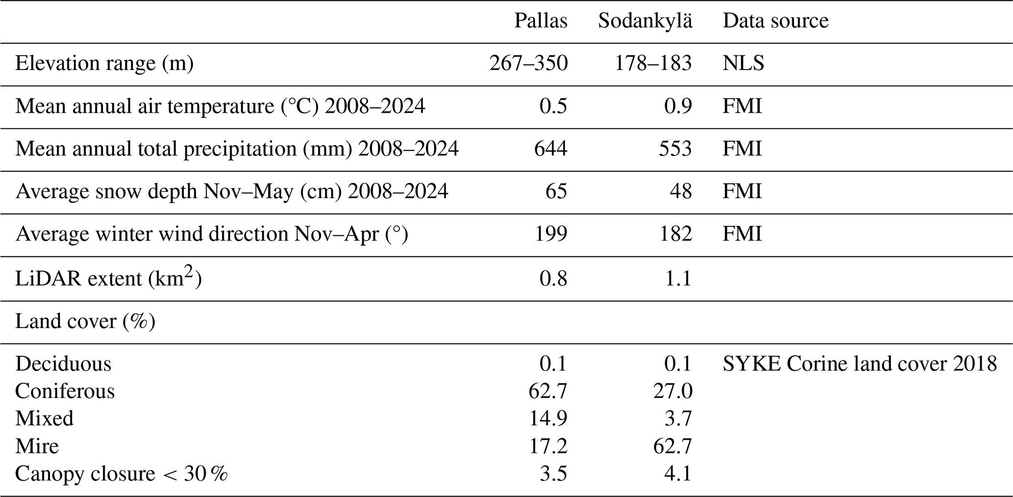
Source: Finnish Meteorological Institute (FMI) (2025), Open data: Snow depth, average temperature, precipitation amount, https://en.ilmatieteenlaitos.fi/download-observations, last access: 3 March 2025. Source: Syke (2018), Open data: Corine Land cover 2018 20m, https://www.syke.fi/en/environmental-data/downloadable-spatial-datasets#corine-land-cover, last access: 3 June 2024, National Land Survey of Finland (NLS) (2020).

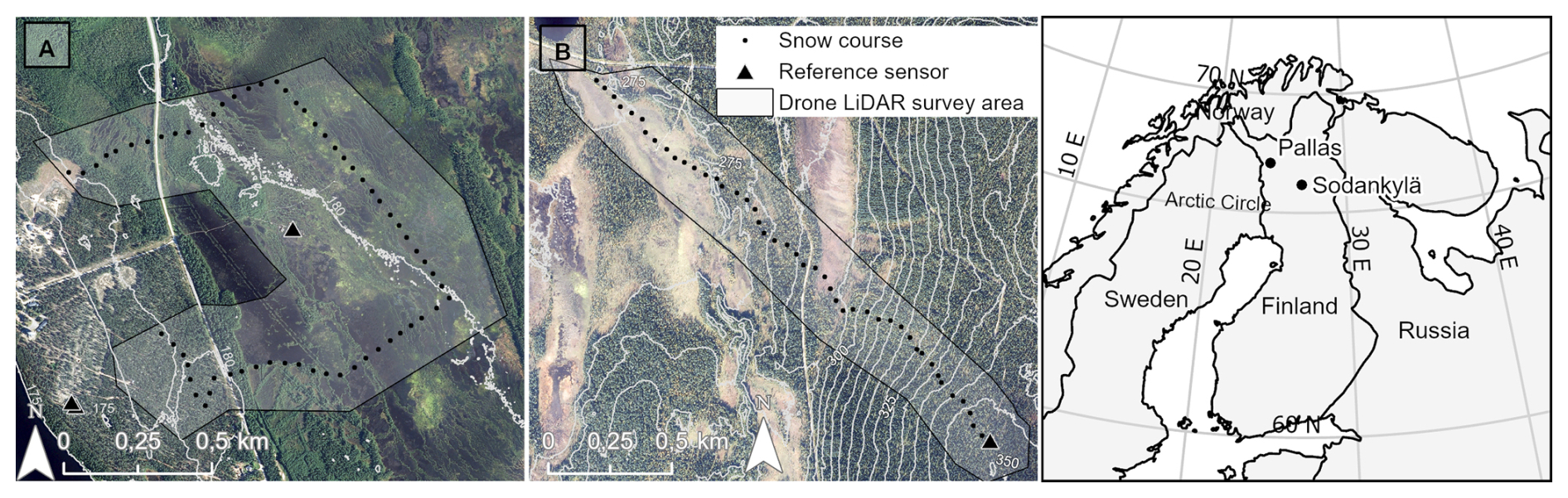
Figure 1 The location and maps of study sites (a) Sodankylä and (b) Pallas. The grey area represents UAV flight areas, and the black points mark the manual snow sampling locations of the snow courses. Orthophotos were obtained from the National Land Survey of Finland.

2.2 Field measurements

In our field campaigns, one snow-off and four snow-on LiDAR surveys were conducted at both sites during the winter of 2023–2024. Snow-on campaigns were carried out at the beginning of January, the end of March, the end of April, and the beginning of May, whereas the snow-off campaigns were conducted on 30 May for Sodankylä and 7 June for Pallas, just after snowmelt and before the new vegetation growth season. The aim was to capture the snowpack in its different winter stages – (i) new snowpack, (ii) maximum snowpack, and (iii) late melting snowpack – to distinguish areas in each site with similar snow patterns and variability (Fig. 2). During winter 2023–2024, the snow depths were above the average in Pallas and Sodankylä. At both sites, snow ablation started in March 2024, interrupted by some major snowfall events in April 2024 (see Fig. S4 in the Supplement).

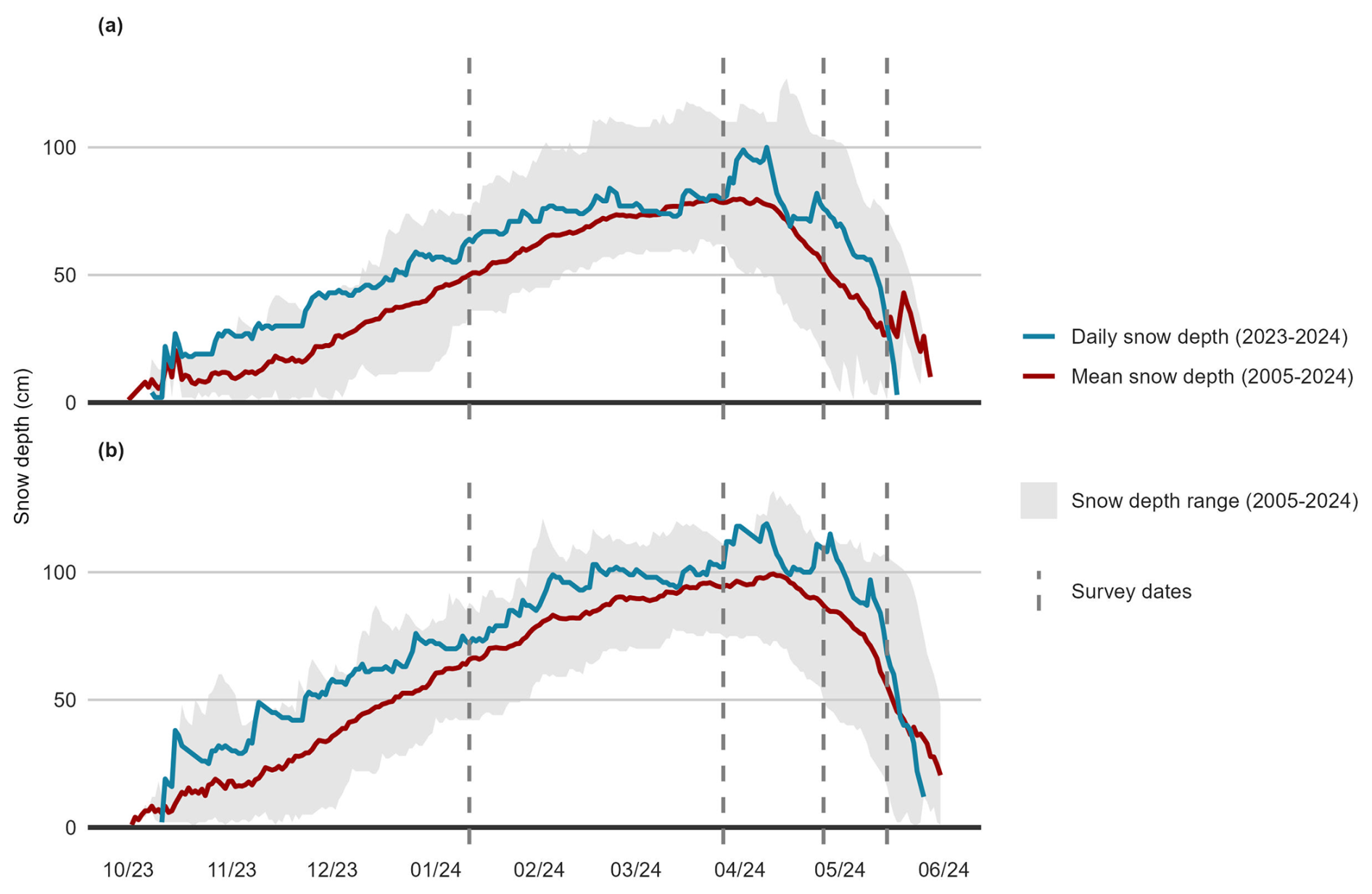
Figure 2 Snow depths from each site's FMI stations. Sodankylä (a), and Pallas (b). Dark dashed lines represent the UAV campaign dates from the winter of 2023–2024. The red line represents the long-term average snow depth (2005–2024), and blue lines the daily snow depths of this study's winter season 2023–2024.

2.2.1 UAV LiDAR surveys

UAV LiDAR mapping was performed at Sodankylä and Pallas using YellowScan Mapper+ (YellowScan, France), equipped with an Applanix APX-15 inertial measurement unit and mounted on a DJI Matrice 300 RTK (DJI, Shenzhen, China). The scanner operated with a 70.4° scanning angle and a 240 kHz pulse repetition frequency, with both sites scanned at a cruising speed of 7 m s⁻¹, at an altitude of 80 m above ground level, and with a 70 % overlap between flight lines (Table S1 in the Supplement). Trajectory correction was carried out in Applanix POSPac software using continuously operating reference station (CORS) observations from the National Land Survey of Finland CORS network as the reference data. For more details on the LiDAR system and flight parameters, see Table S1 in the Supplement.

We compared the accuracy of the digital terrain models (DTMs) between different data processing methods, using five GCPs (ground control points) as a reference. In YellowScan CloudStation, we tested two gridding strategies for DTM generation – MinZ, which uses the minimum elevation value within each grid cell, and MeanZ, which averages the elevation of all ground points for each cell. We also compared the accuracy of the DTMs between different data processing methods, using 5 GCPs (ground control points) as a reference. The 5 GCP plates were distributed across the study areas during each campaign and geolocated with RTK GNSS devices, Emlid RS2+ (Hungary), or Trimble GNSS system R12i (USA), which report 7–8 mm horizontal and 14–15 mm vertical RTK accuracies. The best results were obtained when processing the point clouds with the MinZ method, which was therefore used for the determination of DTMs from the point clouds.

2.2.2 Manual snow measurements

Manual snow depth and density measurements were conducted within 6 h of the completion of the UAV campaigns. Snow course measurements were carried out following the SYKE snow survey protocol (Kuusisto, 1984; Mustonen, 1965; Kuusisto, 1984; Mustonen, 1965). Snow depth was measured every 50 m and density every 200 m along the snow course transect in Pallas (Fig. 1a). In Sodankylä, where the snow course is longer (4 km), SWE was measured at eight different sites along the snow course. These measurement locations were selected to represent different terrain types present in the study site (Fig. 1b). Snow measurement points were geolocated using RTK GNSS Emlid RS2+ (Hungary) and Trimble GNSS system R12i (USA). In Pallas, snow depth was measured using fixed poles installed in the field, whereas in Sodankylä, measurements were taken manually with a wooden snow probe at predefined GPS-marked locations. The data obtained were used as validation data for modelled maps.

2.2.3 Automatic daily snow depth measurements

Sodankylä is equipped with three ultrasonic sensors (Campbell Scientific SR50) providing daily snow depth recordings (Fig. 1b). The sensors are operated by FMI, and the data are open access (https://litdb.fmi.fi/index.php, last access: 5 March 2025). Sensors are in open peatland (67°22.024^′ N, 26°39.070^′ E), in pine forest openings (67°21.706^′ N, 26°38.031^′ E), and inside sparse pine forest (67°21.699^′ N, 26°38.051^′ E). Pallas has one ultrasonic sensor (Campbell Scientific SR50) providing daily snow depth data. This sensor is located in Kenttärova (Fig. 1a) and is also operated by FMI (https://en.ilmatieteenlaitos.fi/download-observations, last access: 5 March 2025). The sensor is located in the spruce forest in the upper part of the study area (67°59.237^′ N, 24°14.579^′ E).

2.2.4 Associating manual snow course measurements with automatic snow depth sensors

Manual snow depth measurements from snow courses were linearly interpolated to estimate snow depths between measurement dates. To improve the accuracy of these estimates, the interpolated values were adjusted using daily snow depth changes recorded by the in situ snow depth sensors (Fig. 1a, b). At each snow course measurement point, the interpolated snow depth was corrected by adding the daily change observed at the representative snow depth sensor. Unlike Pallas, where one reference sensor is available, Sodankylä has multiple ultrasonic snow depth sensors distributed across different environments, allowing more representative corrections. Each snow course measurement point is assigned to one of these environmental categories, ensuring that the most appropriate sensor was used for correction. If the corrected snow depth estimate resulted in a negative value, it was set to zero.

2.3 Data analysis

2.3.1 LiDAR data processing

LiDAR data from each campaign were pre-processed using CloudStation software. As part of this process, we performed strip alignment of the flight lines to generate an accurately georeferenced point cloud. To classify points belonging to the ground, we applied the following parameters: steepness (which reflects terrain variation) was set to 0.2, the minimum object height (the vertical threshold above which an object is not considered part of the ground) was set to 0.03 m, and point cloud thickness was set to 0.15 m. Multiple combinations of parameters – such as minimum object height and slope tolerance – were tested and visually evaluated against field observations and GCPs. The final configuration effectively minimized misclassification and produced the most accurate and realistic DTMs for our boreal study area. The same parameter set was applied consistently across all campaigns, including both bare-ground and snow-covered conditions. Although snow accumulation can smooth terrain features and influence classification (e.g. reducing local slope), the selected settings yielded stable and reliable results across all conditions.

Following classification, we generated DTMs with a 10 cm spatial resolution. MinZ-method-based DTM showed better correspondence with the GCP plates (Sect. 2.2.1) and was used in the following analysis. The DTMs generated using this method for the May campaign in Sodankylä showed lower accuracy compared to those produced by other methods. Nevertheless, as the DTMs from the other campaigns and sites were the most accurate when processed with CloudStation, we chose to apply the same method consistently across all sites and campaigns, accepting the reduced accuracy for May. In addition, for each campaign, the point cloud data show increments along the trajectory line borders of approximately 1–5 cm. The uplifts are presumably due to poorer georeferencing of points at the trajectory edges, and presumably overlapping points from the two trajectories can cause abnormal surfaces in DTMs. We tried to clean up the data from overlapping points, but the overall accuracy of the DTM was degraded, so we chose to accept the inaccuracies in the UAV flight trajectory edge regions.

Further DTM processing was conducted using ArcGis Pro 3.2.0. The snow depth rasters were generated by calculating the difference between the snow-on and the snow-off DTMs and resampled to 1 m resolution. Snow depth values falling outside a reasonable range ($<-\mathrm{0.5}$ m; >2 m) were set to zero to remove extreme outliers, while minor negative values close to zero were corrected to zero (−0.5 to 0 m). Missing values were filled by calculating the median value from surrounding cells, using the median of the 5×5 neighbouring cells. The data were clipped to the area of interest (AOI), focusing the analysis on the buffer zone of 150 m around the snow courses. The 4 DTMs were then stacked together to be used as an input for the model (Sect. 2.3.2).

The error metrics were calculated using the 5 GCPs distributed in the study areas to compare their accuracy to the derived DTMs following the suggestion of Rauhala et al. (2023). To estimate the uncertainty in generated DTMs, the difference between UAV DTMs and RTK-measured GCP elevation (Δz) was calculated following Eq. (1):

$$\begin{array}{}\text{(1)}& \mathrm{\Delta }{z}_t={\text{DTM}}_{{\text{s}}_t}-z_{\mathrm{GCP}}t,\end{array}$$

where t is the date of survey, DTM_s is the snow surface elevation from the UAV survey, and z_GCP is the GCP elevation measured with RTK.

When the snow depth rasters were derived from two DTMs, their precision was estimated following Eq. (2):

$$\begin{array}{}\text{(2)}& \mathit{u}=\sqrt{\mathit{\sigma }{\left(\mathrm{\Delta }{z}_t\right)}^{\mathrm{2}}+\mathit{\sigma }{\left(\mathrm{\Delta }{z}_{\mathrm{G}}\right)}^{\mathrm{2}}},\end{array}$$

where σ(Δz_t ) is the standard deviation for the difference between the UAV DTM and RTK-measured GCP elevation Δz for every winter campaign and σ(Δz_G) is the standard deviation for the difference between the UAV DTM and RTK-measured GCP elevation Δz for the bare-ground campaign.

To estimate the trueness of the calculated snow depth rasters, error propagation for the mean error of snow-on and bare-ground DTMs was calculated. It is calculated by finding the average of the differences between the UAV DTMs and the GCP elevations, following Eq. (3):

$$\begin{array}{}\text{(3)}& m=\mathit{\mu }\left(\mathrm{\Delta }{z}_t\right)-\mathit{\mu }\left(\mathrm{\Delta }{z}_{\mathrm{G}}\right),\end{array}$$

where μ(Δz_t) is the mean error for the difference between each snow-on campaign's DTMs and GCPs and μ(Δz_G) is the mean error for the difference between bare-ground campaign DTMs and GCPs.

2.3.2 Application of ClustSnow to LiDAR datasets

We applied the ClustSnow workflow first presented in Geissler et al. (2023) to our dataset. All analyses were performed using R statistical software (v.4.3.0, R Core Team, 2023). To obtain clusters, ClustSnow applies the k-means (Hartigan and Wong, 1979) and random forest (Breiman, 2001) algorithms to a stack of snow depth (SD) rasters. Consequently, the obtained clusters only rely on multitemporal snow observations and do not contain information on the canopy or topography. As a first step, the k-means algorithm groups a small subsample of cells based on their similarity of observed snow depths into a user-defined number of clusters. Secondly, these subsampled and clustered points are used to train a random forest model that, as a last step, is used to predict the probabilities (w) of all grid cells (ij) belonging to the individual clusters (c). Hereafter, we refer to the ClustSnow output as cluster probabilities (w_ij,c), and the map containing the cluster numbers for each cell with the highest predicted probability is referred to as the cluster map. Cluster numbers are ordered based on the mean snow depth of the underlying SD raster stack to allow easier interpretation and comparability. Therefore, a cluster number of one is assigned to the cluster with the highest mean snow depth, and the numbering increases with mean snow depth until the user-defined number of clusters is reached.

2.3.3 Creating daily SD and SWE maps

Cluster probabilities at the snow course measurement locations (ij=s) (w_s,c) are assigned by normalizing so that they sum to 1 in each cluster according to Eq. (4):

$$\begin{array}{}\text{(4)}& \widehat{w_{s,c}}={\displaystyle \frac{w_{s,c}}{\sum _s\left(w_{s,c}\right)}}.\end{array}$$

The synthetic daily snow depths for each cluster SD_c(t) are calculated by multiplying the normalized probabilities by the snow depth values of the corresponding snow course measurements and summing them for each cluster according to Eq. (5):

$$\begin{array}{}\text{(5)}& {\text{SD}}_c\left(t\right)=\widehat{w_{s,c}}\cdot {\text{SD}}_s\left(t\right).\end{array}$$

The synthetic snow depth maps SD_ij(t) are generated by combining synthetic daily snow depth data (SD_c(t)) with cluster probabilities w_ij,c and multiplying them with the time series data of that cluster (SD_c(t)) according to Eq. (6):

$$\begin{array}{}\text{(6)}& {\text{SD}}_{ij}\left(t\right)=\sum _c(w_{ij,c}\cdot {\text{SD}}_c(t\left)\right).\end{array}$$

The synthetic daily snow depth data for clusters were converted into SWE using a semi-empiric Δ snow model (Winkler et al., 2021). The model consists of four modules, namely new snow and overburden, dry compaction, drenching, or scaling modules, and each module is activated depending on the change in snow depth between time steps. The model has seven parameters to be calibrated, and Fontrodona-Bach et al. (2023) suggested that two of them are significantly related to the site-specific climate variables. These two key parameters are the maximum density of a snow layer (ρmax) and new snow density (ρ0). Only Sodankylä has snow measurements allowing the determination of ρ0. At other sites the model was run with the values of ρ0 and ρmax provided by Fontrodona-Bach et al. (2023). The rest of the seven parameters were kept as the default values in Winkler et al. (2021).

The daily SWE maps SWE_ij(t) are calculated using the synthetic snow depth data SD_c(t) as an input for the model and then using the same protocol as for SD maps to upscale the daily SWE estimates for the entire study area using Eq. (7):

$$\begin{array}{}\text{(7)}& {\text{SWE}}_{ij}\left(t\right)=\sum _c(W_{ij,c}\cdot {\text{SWE}}_c(t\left)\right).\end{array}$$

2.3.4 Model calibration and sensitivity

ClustSnow requires a set of parameters to be defined by the user. Most of these parameters showed no sensitivity in the calibration performed in Geissler et al. (2025). The only and most sensitive parameter of ClustSnow is the number of clusters (n_class) parameter. Different indices were tested to guide this decision using the NbClust R package (v3.0.1; Charrad et al., 2014). For Sodankylä and Pallas, these indices suggested an optimal number between one and eight. Besides these indices, we performed a full sensitivity analysis of the ClustSnow workflow following Geissler et al. (2025). Therefore, all model parameters are varied within reasonable ranges and the model was run 1000 times with randomly chosen parameter combinations. The snow products of all model runs are evaluated against manual measurements to obtain the mean and variance of different goodness-of-fit metrics (RMSE, MAE, R). The results of the sensitivity analysis performed are presented in Fig. S1 in the Supplement.

Based on these results, and the low sensitivities of all parameters, parameter values suggested by Geissler et al. (2023) were used, with the exception for the number of clusters (n_class). For comparability and because of the relatively low topographical variation in our sites, we selected n_class to be three in this study for both sites. This number is lower compared to the four clusters obtained in Geissler et al. (2023, 2025) but allows an easier comparison with topographic or vegetation. Yet, to allow a better discussion of the effect of this key parameter on the results, we reran our analysis with n_class set to the optimum of six, obtained in the sensitivity analysis performed here for comparisons (see Sect. 3.3.2).

3 Results

3.1 The accuracy of UAV-based LiDAR for mapping snow depth in boreal and sub-arctic zones

At all study sites, the snow depth measured from snow courses increased until March, after which it started to decrease due to spring melting (Table 2). Snow depth variation increased during the melting season, but in the April and May campaigns, the variability stabilized as snow had already melted in most areas. The uncertainty in the derived DTMs was studied by comparing GCP points to the UAV DTMs (Sect. 2.2.1). The difference between UAV LiDAR snow depth maps and RTK-measured GCPs (Eq. 1) resulted in varying accuracies between sites and campaigns, and their RMSEs can be seen in Table 3. Weather conditions as well as the accuracy of RTK signals might cause differences not directly related to the UAV LiDAR.

Table 2 Mean snow depth and SWE values and their standard deviations from manual snow course measurements in different campaigns and sites in winter 2023–2024.

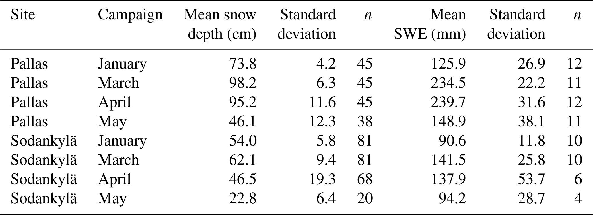
Table 3 The RMSE of the differences between GCP plates and DTMs and the precision and trueness of snow depth maps derived from DTMs in different campaigns and at different sites (Eqs. 1, 2, 3).

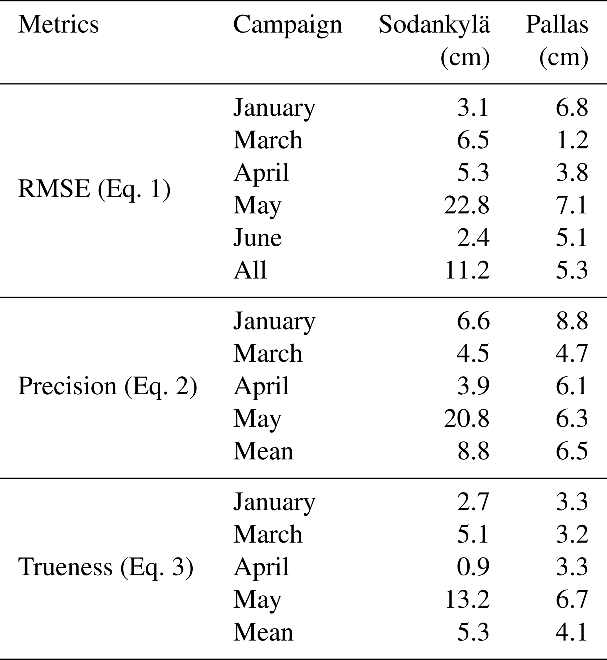
Table 3 also summarizes the precision of snow depth maps from standard deviations for each site calculated by Eq. (2). The precision of the snow depth maps in Sodankylä was stable during the winter campaigns, performing best in April (4.5 cm), but had an uncertainty of 20.8 cm in May. In Pallas the precision ranged from 4.7 cm in March to 8.8 cm in January. The error propagation for mean error, meaning the trueness of snow depth maps calculated by Eq. (3), is also presented in Table 3. In Sodankylä, the trueness was the best in April (0.9 cm), decreasing in May with values of up to 13.2 cm, mostly caused by the computation of the DTM with flooding of the mire areas. Pallas also had the highest trueness at the beginning of winter with relatively stable accuracies through the winter, ranging from 3.2–3.3 cm in January–April and decreasing in May to 6.7 cm. During the main melting season, localized open water and flooding areas, especially in open peatland, cause laser beams to reflect differently in comparison to snow or ground surfaces, which can lead to uncertainties, especially when using the minimal-elevation-derived products. This can therefore affect the quality of May DTMs, making them poorer in comparison to those of other months.

3.2 Cluster characteristics show similarities between sites

The characteristics of clusters derived using ClustSnow and their associated snow conditions at each site were analysed by grouping snow course measurements and environmental data according to their respective cluster classifications.

3.2.1 Cluster characteristics at Sodankylä

Cluster 1 covers 21 % of the total Sodankylä area, typically located in forests or pine mires (Fig. 3). It has an average canopy height of 4.6 m and is located typically less than 1 m away from forests (Table 4). This cluster has the highest average modelled snow depth and SWE through the winter. According to the ClustSnow-derived snow products, peak snow depth occurred on 14 March 2024 at 75 cm and peak SWE on 23 April 2024 at 164 mm (Table 4). The ablation started after the peak, but snow depth increased again at the end of April due to heavy-snowfall events, decreasing rapidly afterwards. From snow course measurements, the points classified into this cluster showed their snow depth peak on 26 March 2024, with an average of 72.5 cm snow depth (see Fig. S2 in the Supplement). None of the 7 SWE measurement points of the snow course were classified into this cluster (Fig. 3).

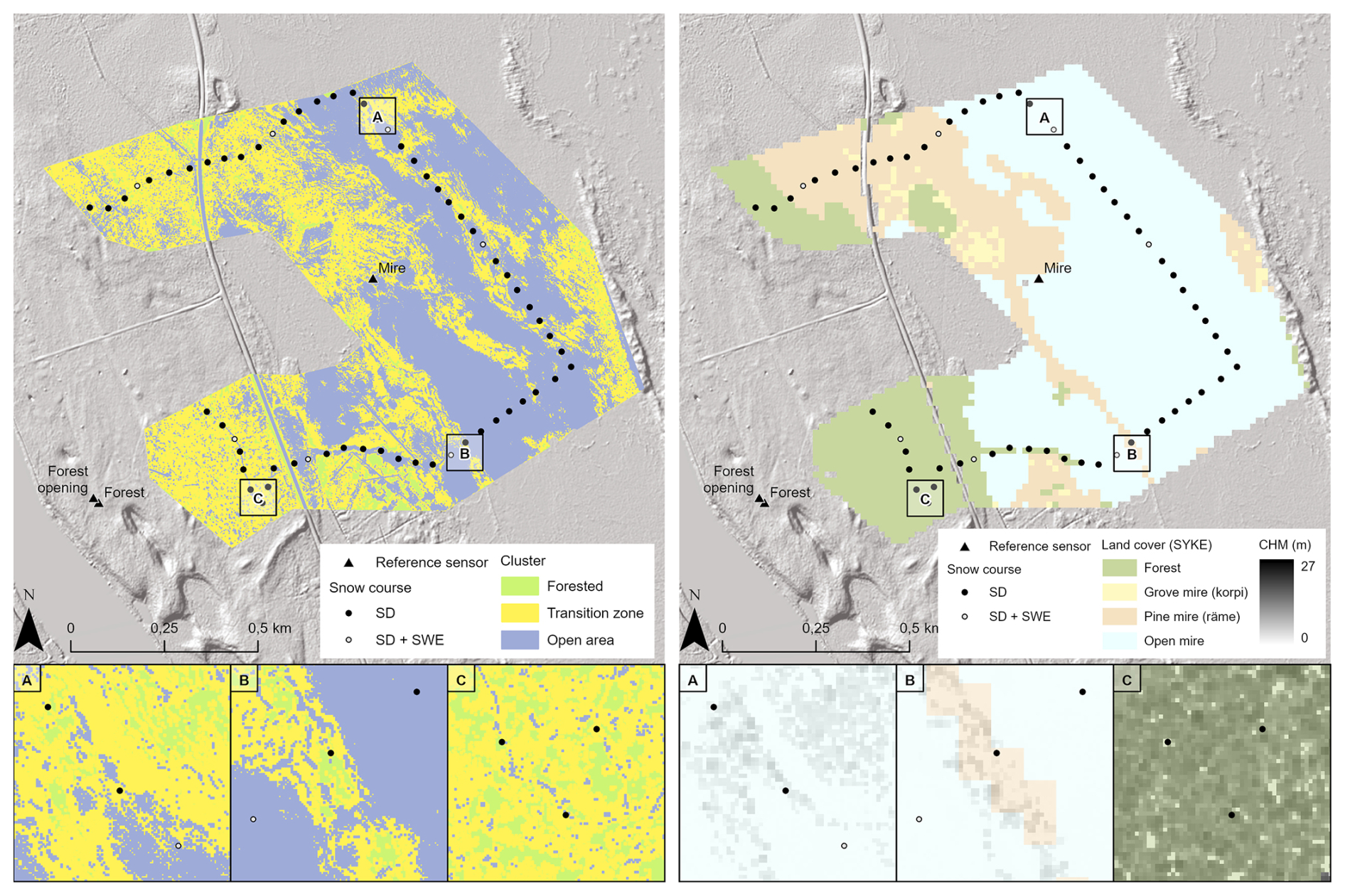
Figure 3 Sodankylä site cluster and vegetation characteristics. Bounding boxes A, B, and C are examples of different cluster zones in relation to their canopy height and land cover.

Table 4 Cluster characteristics in relation to the entire study area of both sites.

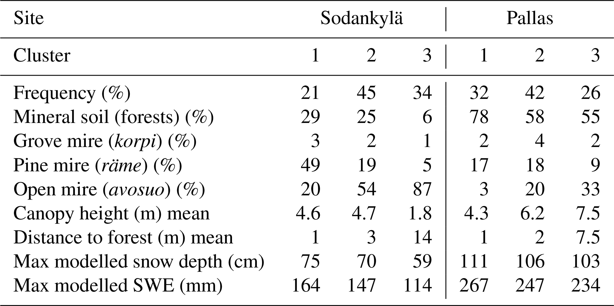
Cluster 2 is the most common, covering 45 % of the total area, and is primarily located in the transition zone between forest and open areas, including forest gaps, mire edges, and forest–mire boundaries (Fig. 3). This cluster has a mean canopy height of 4.7 m and is on average 3 m away from cells classified as forests (Table 4). The modelled peak snow depth occurred on 14 March 2024 (70 cm) and peak SWE on 23 April 2024 at 147 mm (Table 4). Snow course measurements that are classified as cluster 2 have their snow depth peaking on 15 March 2024, with an average of 67 cm, and SWE peaking on 24 April 2024, with an average of 166 mm (see Fig. S2 in the Supplement).

Cluster 3 predominantly occurs in open areas with a low canopy height, with 87 % of the area classified as open mire. This cluster consistently exhibits the lowest snow depths and SWE values compared to the others (see Fig. S2 in the Supplement). The highest modelled snow depth and SWE values for cluster 3 are at the same time as for other clusters, snow depth peaking on 14 March 2024 (59 cm) and 23 April 2024 (114 mm). The snow course snow depths and SWE from cluster 3 both peaked on 15 March 2024, with an average snow depth of 57 cm and SWE of 138 mm.

3.2.2 Pallas snow depth and SWE clusters

In Pallas, the three clusters derived from snow depth maps show similar characteristics to those in Sodankylä (Table 4). The more common cluster, cluster 2, covers 42 % of the study area, with cluster 1 covering 32 % and cluster 3, as the smallest, covering 26 % of the area. The snow depth in the Pallas snow course began to decrease as early as late February across all clusters (see Fig. S3 in the Supplement). This decline was less pronounced in points classified as cluster 1 compared to the other two clusters. However, the timing of peak SWE, marking the onset of snowmelt, was later in the spring compared with snow depth and varied among the clusters.

Cluster 1 is predominantly located in the forested areas, which accounts for 78 % of the cluster, while the open areas cover only 3 % (Table 4). The mean canopy height is approximately 4.3 m, and the distance to the forest cells is less than 1 m, which is less than in other groups, suggesting smaller and denser forest types. Until January, the modelled snow depths for cluster 1 followed similar snow depths to the other clusters, but after February they surpassed those of other clusters and remained the highest until the end of the season (see Fig. S2 in the Supplement). Changes in the snow depths between February and March were small, with occasional fluctuations. The modelled snow depth of cluster 1 peaked on 28 March 2024 (111 cm), and the SWE peaked on 10 May 2024 with SWE of 267 mm. Snow measurements from the snow course show that points classified into this cluster had their peaks in snow depth on 22 February 2024 and 25 April 2024, with both having an average snow depth of 102 cm and SWE on 25 April 2024 of 265 mm.

Cluster 2, identified as a transition zone, is typically located near forest edges, forest openings, and small-scale open mire areas (Fig. 4). Forested areas cover 58 % of the cluster, while open mire areas contribute 20 %. The mean canopy height is approximately 6 m, with a 2.2 m distance from the forest edges (Table 4). The snow depth patterns for this cluster aligned with those of other clusters until late February, after which the snow depths in cluster 2 started to decrease. The modelled snow depth peaked in mid-March on 18 March 2024 with 106 cm and also on 17 February 2024 with 105 cm. The modelled SWE peaked later, on 28 April 2024 at 247 mm and on 10 May 2024 with a SWE of 248 mm. The results are similar to the manual snow course measurements, where points classified into this cluster had their snow depth peak on 22 February 2024 (101 cm). However, snow course SWE peaked twice, having an average of 227 mm on 27 March 2024 and 233 mm on 25 April 2024.

Cluster 3 covers 26 % of the Pallas area and is marked by a mixture of forest (55 %) and open mire (33 %) environments (Fig. 4). It has the greatest distance from forest cells and the tallest mean canopy height of 7.5 m (Table 4). This cluster is typically found in open mires or high-canopy forests. Modelled snow depths in cluster 3 were initially the highest at the start of the season but exhibited a lower rate of increase compared to the other clusters after January and remained the lowest throughout the rest of the season (see Fig. S3 in the Supplement). The peak modelled snow depth, 103 cm, occurred in late February, on 17 February 2024, after which the snow depth steadily declined. The modelled SWE peak was at the same time as for cluster 2, on 28 April 2024 (237 mm). Snow course snow depth measurements were the highest on 22 February 2024, with an average of 96 cm. SWE measurements from the snow course within this cluster are limited, with only five measurements taken during the melting period in late April and early May. During this period, SWE values were initially low but peaked at 186 mm on 7 May 2024 (Fig. S3 in the Supplement).

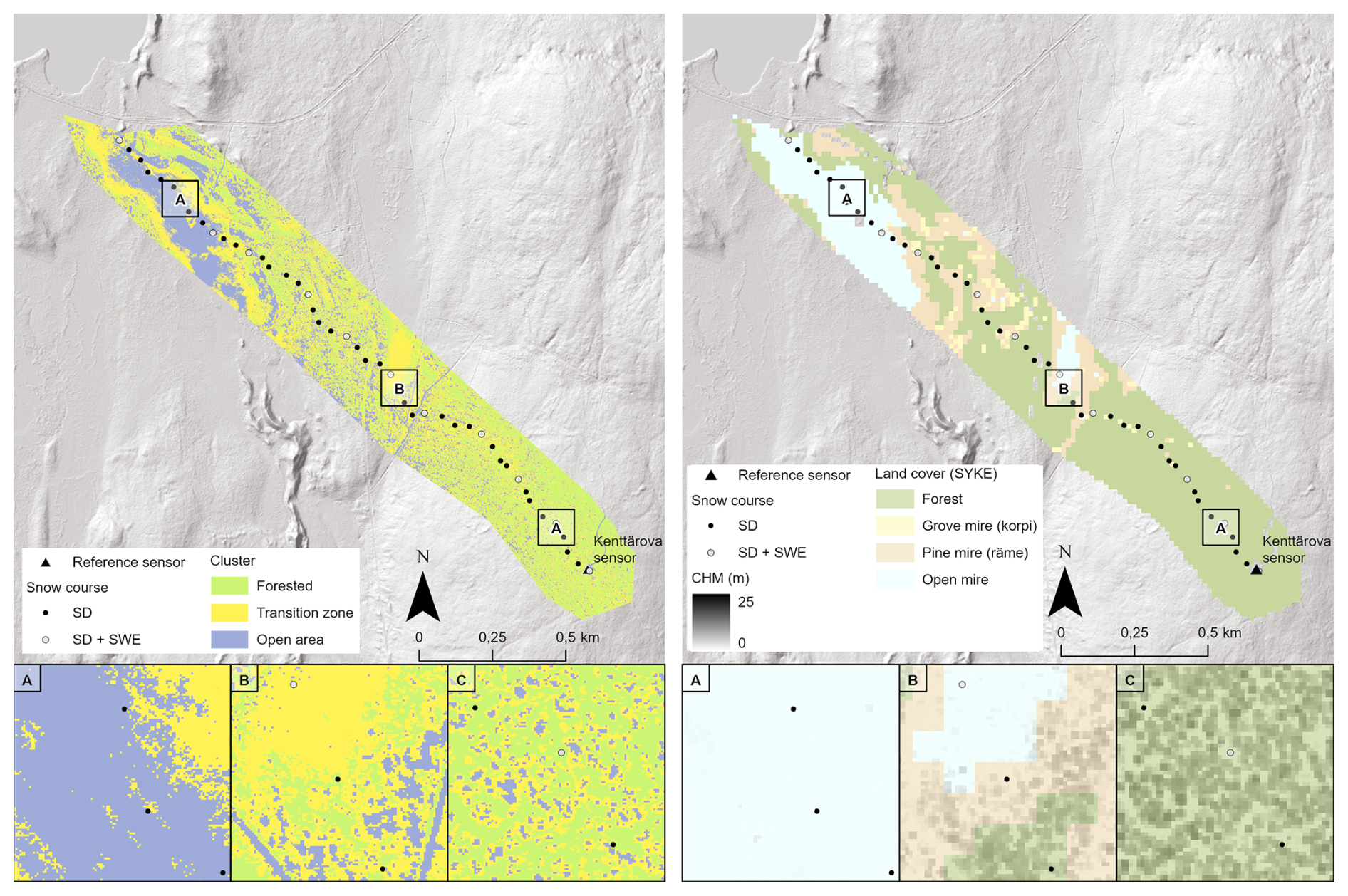
Figure 4 Pallas site cluster and vegetation characteristics. Bounding boxes A, B, and C are examples of different cluster zones in relation to their vegetation.

3.2.3 UAV accuracy in comparison to clusters

To evaluate the accuracy of LiDAR UAV snow depth by cluster in relation to the representativeness of reference snow depth sensors, SD measurements taken during the snow course were assigned to their representative cluster. When comparing the UAV-based LiDAR SD maps and manual snow course SD measurements, the LiDAR maps consistently underestimate the snow course measurements in both Pallas and Sodankylä (Fig. 5a, b). In Sodankylä, all snow course measurement campaigns show similar correspondence to the LiDAR snow depth maps and variations among clusters are similar, showing consistent agreement with snow course measurements (Fig. 5a). In Pallas the snow course measurements classified as cluster 1 correspond the best to the LiDAR snow depth maps, while the largest discrepancies are observed in cluster 3, typically located in wet mire areas (Fig. 5b). The accuracy of UAV LiDAR maps decreases towards the melting season, where, especially in Pallas, the SD estimates are on average 30 cm less than the snow course measurements.

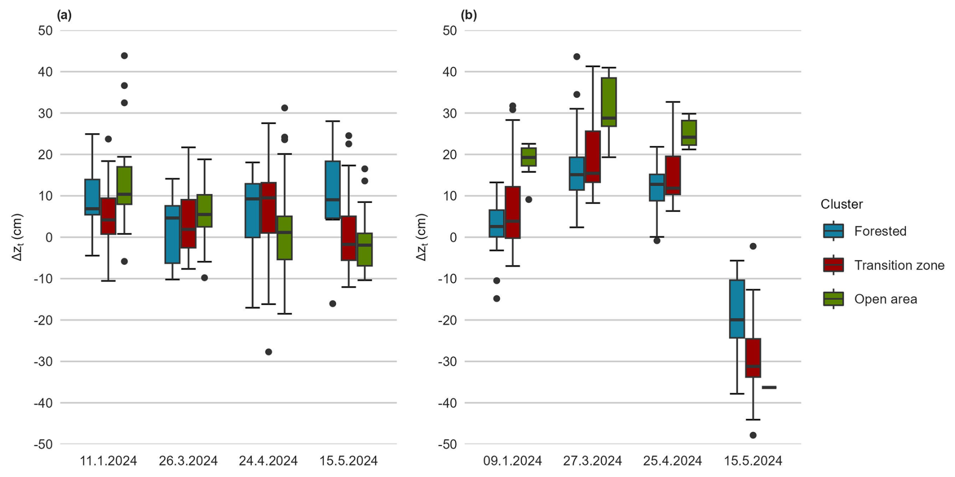
Figure 5 Differences in Δz_t (cm) between the UAV-based LiDAR snow depths and snow course measurements by each campaign and representative cluster in (a) Sodankylä and (b) Pallas.

Snow course measurements and the UAV-based LiDAR snow depth maps for each campaign were compared with the reference snow depth sensor measurements of the study area (Figs. 1, 2) to define the overall representativeness of the measurements and clusters. In Sodankylä, all the aforementioned datasets follow similar patterns: clusters had similar mean snow depths to the sensors and were within the ranges of snow course measurements (Fig. 6a), except in May, when the snow course snow depths matched neither UAV LiDAR nor the sensor snow depths. The largest snow depths were in the forested cluster and from the reference sensor located in the forest opening. In Pallas, the UAV LiDAR snow depth maps underestimate the snow height in relation to both snow course measurements and the reference snow measurement (Fig. 6b). Cluster 1 has the highest correspondence to the snow course and reference sensor compared to the areas classified as other clusters.

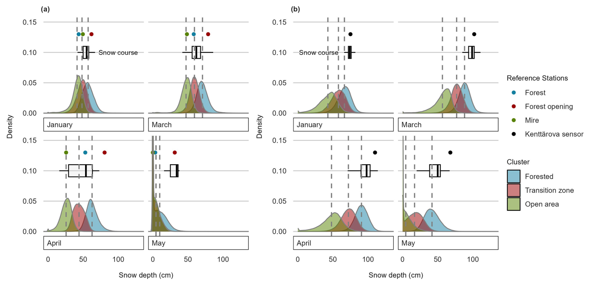
Figure 6 Reference sensor snow depths compared to UAV LiDAR snow depths by cluster in Sodankylä (a) and Pallas (b) in each campaign. Dashed lines are the mean values of snow depths at each cluster.

3.3 Model validation

3.3.1 Comparison of modelling results to snow course data

The model creates daily snow depth and SWE estimates for the two study sites. These estimates were compared to the snow course measurements and UAV LiDAR snow depth maps to estimate their accuracy (Table 5). The snow depth predictions of modelled maps have an overall accuracy of 8.0 cm in Sodankylä and 5.8 cm in Pallas compared to the manual snow course measurements (Table 5). The SWE values differ from snow course measurements in Pallas, with RMSE of 35.6 and 33.1 mm in Sodankylä during all measurements in winter 2023–2024. The predicted SWE values of the Sodankylä snow course follow the observed snow course SWE values (Fig. 7a). The model tends to slightly underestimate the SWE, particularly during the late season, but the median values of measurements fall within the model's predictive range. Model performance is the highest in February, with RMSE of 12 mm (n=7). In contrast, the performance declines towards the end of the season, with RMSE of 73 mm in May (n=4), as can be seen in Table 5.

In Pallas, the modelled SWE values are typically within the range of manual SWE measurement values (Fig. 7b). The model has an overall accuracy of 32 mm (Table 5), with its best performance observed early in the season, with RMSE of 6 mm in November (n=12) and 8 mm in December (n=12), as shown in Table 5. The highest error, 59 mm (n=12), occurs during the onset of the rapid snowmelt in early May. Despite this, the modelled SWE values successfully capture the seasonal peak in April and May, consistent with the snow course measurements.

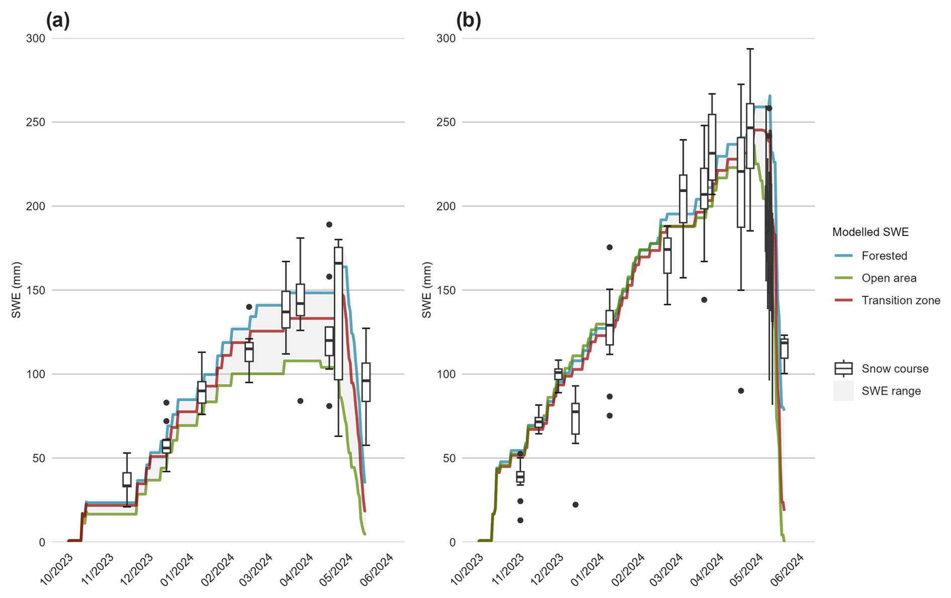
Figure 7 Modelled SWE values in comparison to measured SWE values of the snow course in Sodankylä (a) and Pallas (b) in 2023–2024.

Table 5 RMSE for Sodankylä and Pallas modelled SWE.

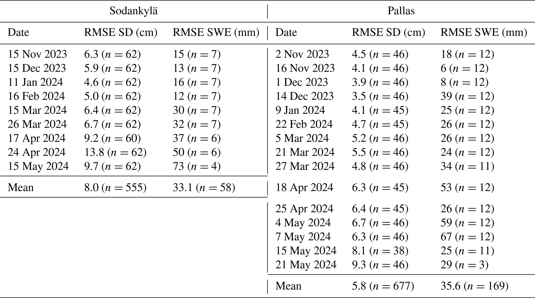
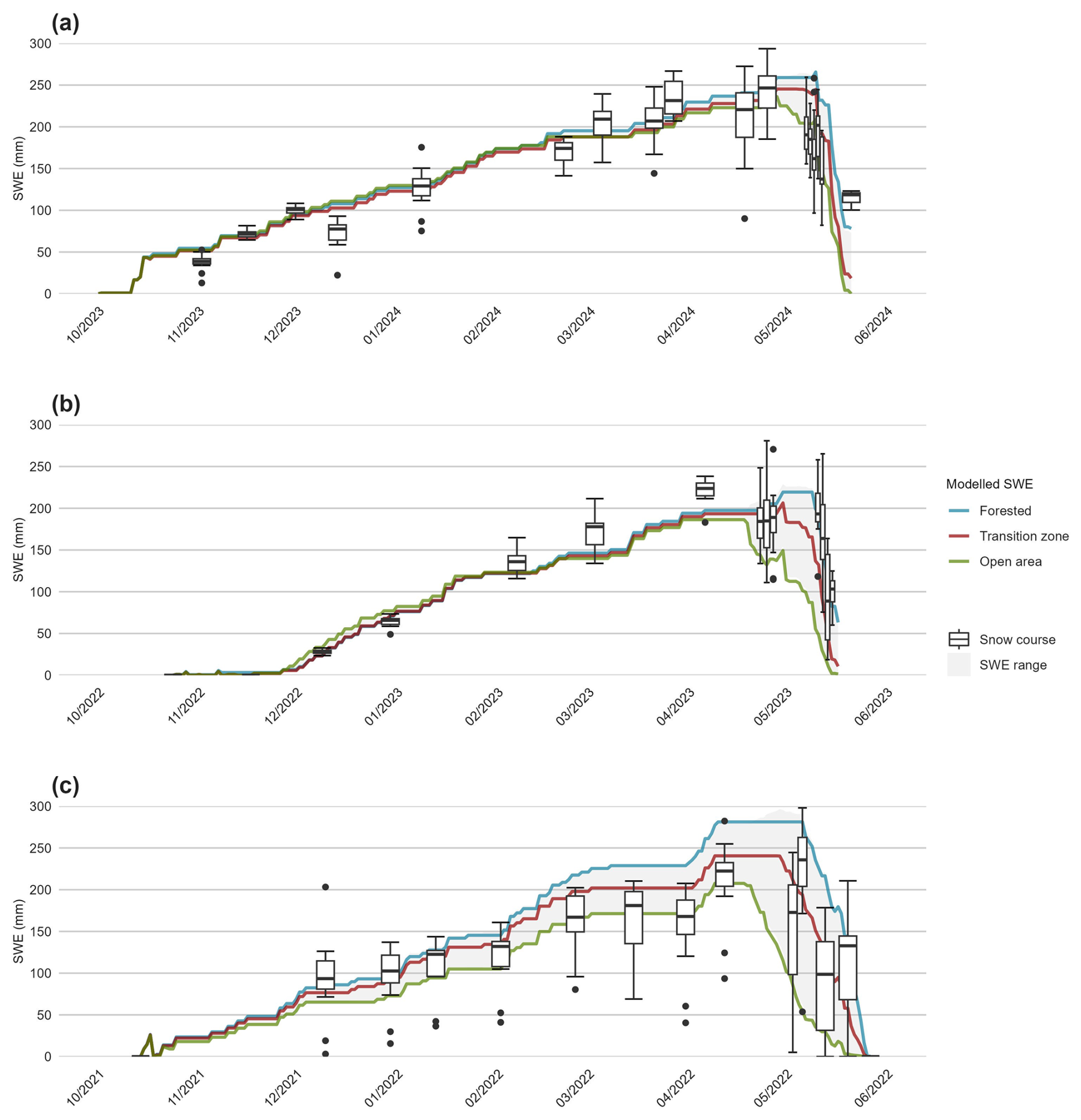
Figure 8 Modelled SWE of the previous winters, (a) 2023–2024, (b) 2022–2023, and (c) 2021–2022, at Pallas in comparison to the snow course SWE measurements.

ClustSnow-derived clusters therefore served as a valid extrapolation basis for snow depth and SWE measurements throughout the entire snow season 2023–2024. Previous application of ClustSnow suggests that these clusters are not only suited to extrapolating measurements of the same season as that of when the cluster's underlying snow depth maps were acquired, but also transferable to other snow seasons (Geissler et al., 2025). Clusters defined by this study's snow dataset of 2023–2024 were therefore used to see how well the model can reproduce previous years' snow course measurements. SWE measurements from previous years are available for Pallas starting from 2021, although the number of measurements varies across years. The results show that SWE values from the winter 2022–2023 snow course are aligned with model estimates, also capturing the peak SWE in late April (Fig. 8b). The winter of 2021–2022 exhibits the greatest variability in snow course SWE measurements, with the model overestimating SWE for most of that winter. In other winters, the model typically underestimates SWE relative to snow course measurements. Additionally, the variance in SWE values across clusters is largest during the winter of 2021–2022, reflecting greater variability in snow depth along the snow course. However, the average of the SWE from the snow course in winter 2021–2022 aligns with cluster 3, and ClustSnow successfully captures the SWE peak at the beginning of May 2022. The model generally captures the snow course median SWE values from the manual measurements, as well as the peak SWE values and their timing in previous winters.

3.3.2 Spatial accuracy of the model is influenced by spring floods and snow wind distribution

Figure 9 visualizes the modelled snow depths for the March campaign in Sodankylä, highlighting the influence of clustering on snow depth predictions. The modelled snow depths align with the observed snow course measurements, but the model struggles to accurately represent extreme high or low values of snow depths captured by the UAV LiDAR. The figure also demonstrates the effect of adding more clusters to the model. For example, 6 clusters would provide more detailed snow depth estimates but would still miss the actual variability in the snow depths. The UAV LiDAR shows the spatial variability in snow depth between snow course measurement points, which is not captured during the snow course measurement survey. To be able to evaluate the model performance spatially, comparisons between modelled snow depth maps and UAV LiDAR maps were conducted for each of the campaigns. First, the difference between the UAV LiDAR SD map and the model SD output was derived (Figs. 10 and 11); the differences were then squared and averaged, and the square root of the mean was calculated to obtain overall RMSE for the campaign and model.

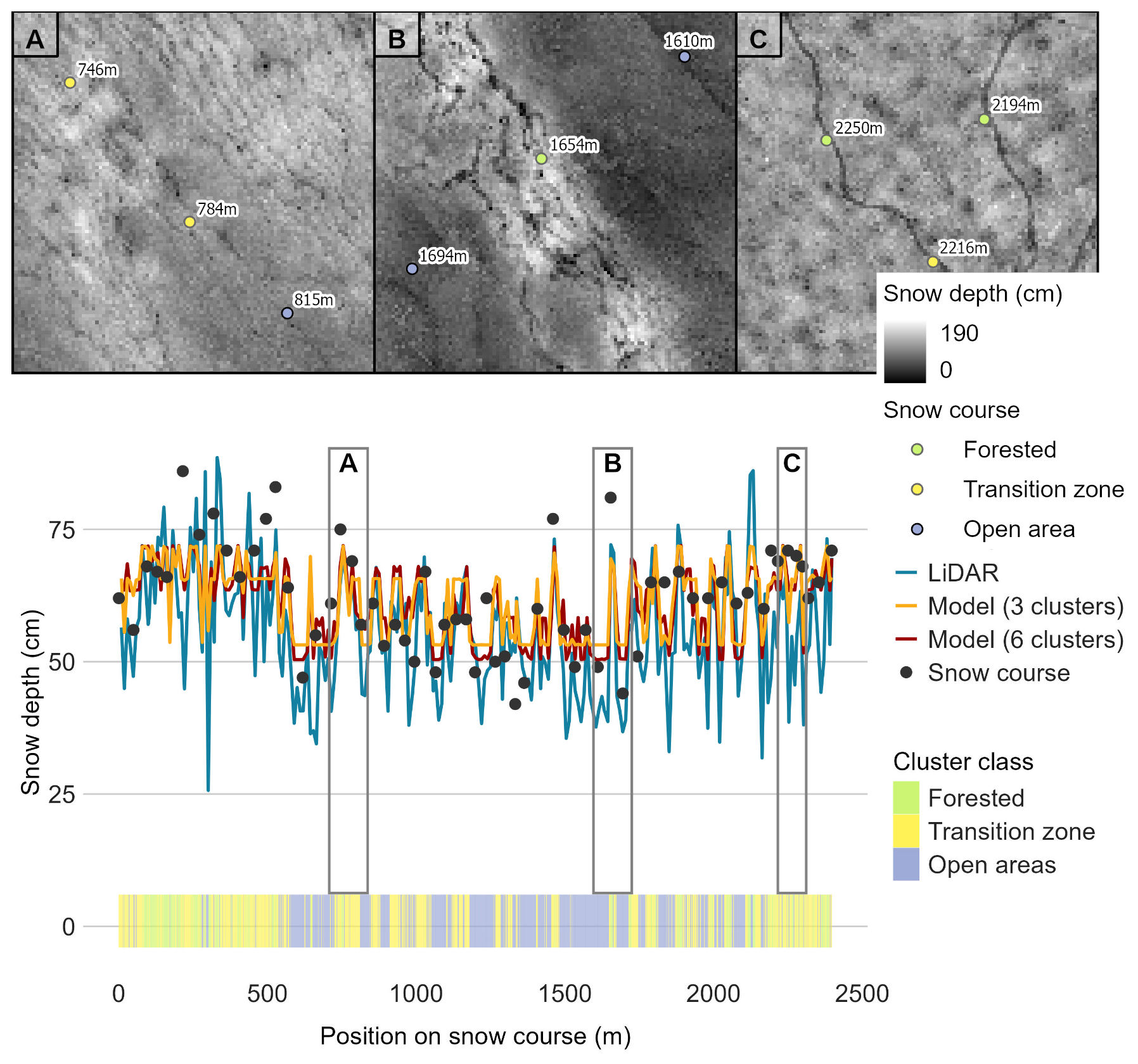
Figure 9 The transect from Sodankylä modelled snow depths, UAV-based LiDAR snow depths, and snow course measurements and their representative clusters on 26 March 2024. The yellow line shows the model output of the model with the number of clusters set to three, as used in this study. For comparisons, the red line represents the model output with the number of clusters set to six.

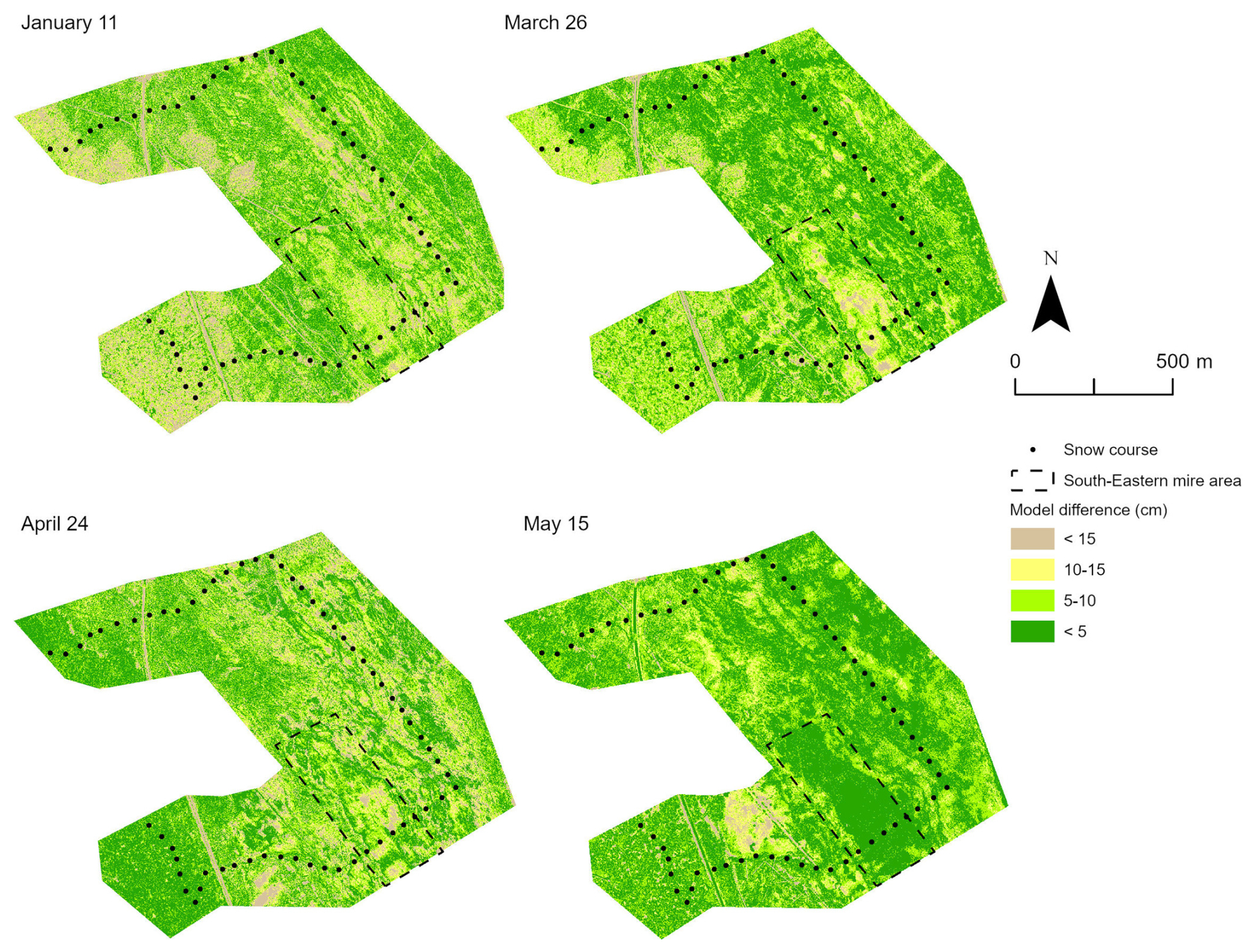
Figure 10 Sodankylä model performance from different UAV LiDAR campaigns. The values define the absolute difference between LiDAR-based snow depth maps and the modelled snow depth maps.

In Sodankylä, the analysis resulted in RMSEs varying from 6.2 to 11.0 cm (January: 11.0 cm; March: 8.2 cm; April: 8.8 cm; May: 6.2 cm). The accuracy of the modelled snow depth maps is influenced more by the timing of the campaign than by the specific location (Fig. 10). For instance, in an open mire area located in the southeastern section of the snow course, the model's performance varies significantly, with differences ranging from 10–15 cm in March and decreasing to less than 5 cm in May (Fig. 10, dashed box). Similarly, in the spruce-dominated forest situated in the southwestern part of the area, the highest accuracy is observed in April (difference <5 cm), whereas in January, the model predictions exhibit a larger discrepancy, with errors ranging from 10–15 cm.

In Pallas, the model has higher inaccuracies compared to Sodankylä, with RMSEs varying from 18.7 to 24.7 cm (January: 22.4 cm; March: 24.7 cm; April: 22.7 cm; May: 18.7 cm). The model therefore performs best at the beginning and at the end of the season. Spatially the model performs best particularly at the southern end of the snow course, characterized by homogeneous pine and mixed forest (Fig. 11). In contrast, the model has the highest errors in the broad Lompolonjänkä mire area in the northeast, where the snow is on top of a flooding mire area, and on the northern slopes of the bordering drumlins, where wind-driven snow accumulation is common. In these areas, the model estimates differences of over 30 cm from the UAV LiDAR map.

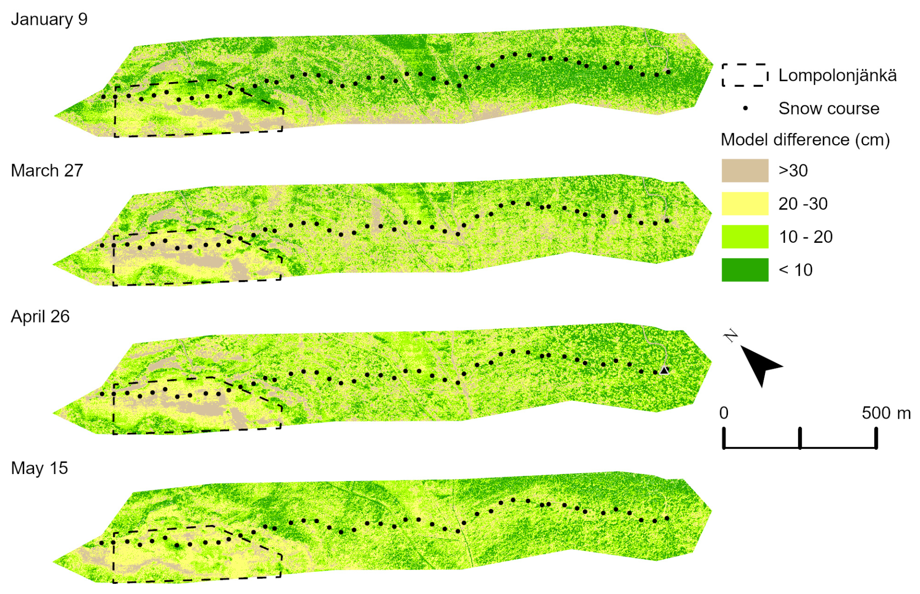
Figure 11 Pallas model performance from different UAV LiDAR campaigns. The values define the absolute difference between UAV LiDAR snow depth maps and the model output.

4 Discussion

4.1 Snow and ice conditions impacted UAV LiDAR accuracy

UAV LiDAR mapping showed high accuracy at all study sites and in all conditions, with the average RMSE of UAV LiDAR DTMs being 11.2 and 5.3 cm for Sodankylä and Pallas, respectively. These results align with previous studies, which have reported RMSE values from snow depth maps ranging from 9 to 17 cm (Dharmadasa et al., 2022; Geissler et al., 2023; Harder et al., 2020; Jacobs et al., 2021). However, our larger uncertainty and lower accuracy were noted, especially in the late melting period with flooding conditions, which might be impacted by laser beam reflection from waterbodies.

The trueness of the snow depth maps derived from DTM maps varies between 0.9–13 cm, and RMSEs of individual DTMs vary between 1 and 7 cm (excluding an outlier in Sodankylä in May of 22.1 cm). The precisions here are based on the 5 GCP measurements suggested by Dharmadasa et al. (2022). Pallas has the most stable conditions, and Sodankylä has the lowest bias in April (0.9 cm). The accuracy of the GCP location measurement itself can affect the accuracy estimates. For example, one measurement in Sodankylä (May) shows a significant difference from the DTM, which decreases the overall accuracy of the site. The point was not excluded from the calculations, as the error may also be due to the DTM calculation errors from flooding areas. The accuracy of UAV LiDAR snow depth mapping is dependent on several factors, which can be divided into boresight errors, navigational errors, terrain- and vegetation-based errors, and post-processing errors (Deems et al., 2013; Pilarska et al., 2016). For example, fallen tree trunks, very dense undergrowth, or flooded marshes can pose challenges to point cloud classification and affect the output DTM quality (Deems et al., 2013; Evans and Hudak, 2007). Similarly, vegetation and terrain affect the accuracy of manual snow depth measurements.

The best accuracy of snow depth maps (0.9 cm) of all sites and campaigns was calculated from the April campaign in Sodankylä. Two days prior to the flight campaign, on 24 April 2024, approximately 10 cm of new snow had fallen in the area, which helped to smooth the snow surface and to cover previously melted or frozen areas under the snow, positively affecting the LiDAR signal and hence the accuracy of the terrain model. In contrast, the trueness of snow depth maps in all sites is lowest in May (Table 3). Our findings highlighted increased measurement inaccuracies during that period, possibly because most of the snow had already melted and large areas were covered with slush and smooth water surfaces. This posed challenges for the DTM algorithm's lowest Z value obtained in the cell, meaning that the height of the reflected laser beams in the water mass also affects the DTM elevations. The trueness values, on the other hand, are based on GCP plates placed in the area, which were located on top of the remaining snow. When the snow is surrounded by water, the model may be inaccurate and produce lower-accuracy DTMs than when the surface is completely covered by either snow or thawed ground. To our knowledge, there is no systematic review on wet snow affecting laser beams. However, water generally has a low reflectivity in the infrared wavelength range compared to solid surfaces, and the return signal detected by the sensor is influenced by factors such as incidence angle and surface roughness (Fernandez-Diaz et al., 2014; Paul et al., 2020). These factors likely contributed to reduced accuracies of the surface detection in areas with localized open water during the melting season. The phenomenon can be seen especially in Sodankylä, which has the largest, typically flooding, mire areas among sites. Results were similar for Rauhala et al. (2023), where the poorest accuracy of SfM-method-based DTMs occurred during the late melting period in flooding areas. This is due to the manual snow course measurements, with these flooding points marked as having zero snow depth and LiDAR-derived snow depth maps still showing snow in these areas. Some vegetation types, such as dense coniferous forests, are known to decrease the accuracy of different UAV methods of snow depth mapping (i.e. Dharmadasa et al., 2022; Rauhala et al., 2023), as coniferous canopy reduces or even prevents ground returns. If we expect cluster 1 to present forested regions and cluster 3 to present open areas with low vegetation and compare the snow depth map accuracies to snow course measurements, we cannot distinguish similar phenomena in Sodankylä or Pallas (Fig. 5). At both sites, the best correspondence between snow course measurements and UAV LiDAR maps is in cluster 2, in forest openings. In contrast, especially in Pallas, the biggest disparities occurred in cluster 3. This may be due to snow course measurement poles being lifted from the ground, especially in wet areas where ground freezing and thawing move the pole over time.

Broxton and van Leeuwen (2020) recommended the SfM method for snow depth monitoring under certain conditions, such as on gently sloping terrain and in areas without dense forest cover. The UAV LiDAR method was selected over the SfM method for this study due to existing dense forest canopy and frequent light conditions that would not allow reliable SfM data acquisition (Rauhala et al., 2023; Revuelto et al., 2021). With advancements in SfM camera technology, the SfM method could complement LiDAR monitoring, particularly in relatively flat regions like Sodankylä and Pallas. Nevertheless, challenges remain for both methods in large mire areas. While the SfM struggles with surface homogeneity, LiDAR faces accuracy issues in detecting bare ground under flooded, uneven, and wet surfaces. Additionally, manual snow depth measurements are also less accurate due to ice and water layers on the ground.

4.2 Site characteristics explaining the different snow depth clusters

Vegetation and topography impacted snow depth clustering in our boreal and sub-arctic sites. Specifically, we noted that canopy cover, open peatlands, and transition zones with wind shelter had a clear and similar influence on the clusters obtained at both sites. Additionally, we noted that the clusters have similar snow dynamics at both sites. The number of clusters has a major impact on the performance of the clustering and ClustSnow and how determined clusters relate to the site's vegetation and topography characteristics.

This study applied ClustSnow with the number of clusters set to three, as initial tests demonstrated their suitability for representing different snow patterns in study areas and three clusters enable us to relate the snow depth patterns to vegetational patterns. An equal number of clusters provides a basis for site comparability between the two study sites. Our analysis resulted in snow depth classification for forests with different trunk heights (cluster 1); transition zones between forests and open areas, including forest edges and gaps (cluster 2); and open areas (cluster 3), mainly peatlands. The results are consistent with those of Mazzotti et al. (2023), who noted that snow accumulation patterns can be classified into three groups, based on the relationship between canopy structure and ablation rate. However, as also noted by Geissler et al. (2025), increasing the number of clusters could, in some cases, improve the accuracy of the end products, and increasing the number of clusters would allow more detailed description of the snow patterns, as can also be seen in Fig. 9. The sensitivity analysis performed for this study's sites confirms this assumption. We found that the highest accuracies of the ClustSnow-derived snow products, evaluated against manual measurements, can be expected with the number of clusters set to six. Especially when the study area has high elevational differences or has various topographical aspects, more clusters would better correspond to the depth patterns. Most uncertainties related to the model parametrization of both models, ClustSnow and Δsnow model, are due to the number of clusters (Fig. S1; see the Supplement).

In forested areas, distinguishing between clusters 1 and 2 remains challenging due to their similar site characteristics (Tables 5 and 6). Forested areas present challenges for clustering because of varying snow height and dynamics influenced by canopy cover and trunk size (Meriö et al., 2023). Forest gaps in the coniferous forests are known to create clear and distinct variations in snow depth within the forests, and SWE varies up to 3 times more in unevenly distributed forests compared to evenly distributed forests (Woods et al., 2006). For this reason, forested areas contained both cluster 1 and cluster 2 at both sites. Cluster 1 receives the most snow and has the highest SWE values, especially during the late winter (Fig. 7a, b). Lundquist et al. (2013) concluded that this is the typical situation in cold climates, where snow lasts longer in forests than in forest openings. At both of our sites, snowmelt starts latest and snow cover lasts longest in cluster 1. The forested areas in Sodankylä and Pallas are spruce dominated, where the canopy not only shades the ground from sun radiation, reduces wind effects, and traps snow, but also limits snowfall reaching the ground. In this cluster, we expect snow accumulation to follow canopy structure throughout the season and the ablation to be too slow or constant to change it, as defined by Mazzotti et al. (2023).

Cluster 2 is the most common cluster at both sites (Tables 5 and 6), likely since it can be found in both forested and open environments. While the snow depth trends across cluster 1 and cluster 2 are similar, cluster 2 experiences an earlier start of snowmelt in spring compared to cluster 1, which is forested (Fig. 7a, b). This indicates more shortwave solar radiation exposure compared to cluster 1, where SWE peaks at the end of April before the melting begins. Cluster 2 characteristics correspond to previous studies, by Koutantou et al. (2022) and Meriö et al. (2023), where the canopy structure influences snow accumulation but in ablation subsequently disrupts these patterns, resulting in earlier timing of snow loss. This can also be seen in the modelling outputs from the previous two winters in Pallas (Fig. 8), especially in winter 2022–2023, when snowmelt in cluster 2 started simultaneously with that in cluster 3. These characteristics are seen at both sites and support the location of cluster 2 as being in transition zones between open and forested areas.

Open areas are subject to wind redistribution and prolonged solar exposure, resulting in lower and smoother snow depth patterns and corresponding to the results of cluster 3. In cluster 3, snow depth starts decreasing notably earlier than in other clusters, in February 2024, suggesting faster melting due to both higher solar radiation and flooding. In the flooding mire areas, melting waters from below also accelerate snowmelt. Both snow depth and SWE values are lower in this cluster in comparison to other clusters, corresponding to results from Meriö et al. (2023). An interesting aspect of the classification is the differentiation between the mires Lompolonjänkä (Fig. 4, box A) and Välisuo (Fig. 4, box B). Välisuo mire, classified as cluster 2, is more sheltered, is surrounded by forests, and is located at a higher altitude than the Lompolonjänkä mire, which is classified as cluster 3. Välisuo is drier and partly artificially drained, while Lompolonjänkä is drained by a small natural stream, typically flooding in spring (Marttila et al., 2021).

The clustering results support the results of other studies on snow distribution in boreal and sub-arctic sites. They also support the ability of ClustSnow to model various environments and sites, in both the Alps and the Arctic boreal zone. Moreover, the results suggest that ClustSnow is generally transferable to large sites as well as to the Arctic boreal climate. In a recent study from the Pallas site by Meriö et al. (2023), the variations in snow depth were partially explained by canopy interception, longwave radiation emitted by trees, and wind-driven redistribution, which contributed to snow deposition along forest edges in both forested and peatland environments. The snow depth was higher within dense canopy, with the greatest accumulation observed in coniferous forest areas, followed by mixed forests, transitional forest–shrubland, and open peatlands. In both Sodankylä and Pallas the dominant winter wind direction is from the south, which leads to snow accumulation in forest canopies, especially on their leeward sides, where typically the largest snow depths are measured, corresponding to the results from Dharmadasa et al. (2023). In Pallas this results in snow accumulating particularly behind the drumlins north of the Lompolonjänkä mire (Fig. 4, box A). This is also reflected in the accuracy of the model in these areas – the three clusters may not be sufficient to account for the particularly large snow depths of the northern sheltered slopes (Fig. 11). In comparison, snow dynamics in Sodankylä are influenced by vegetation rather than by topographical variations, as the area itself is flat with elevation differences of less than 2 m. Forest structure is the main driver of snow accumulation, but shortwave radiation can disrupt these patterns, especially on south-facing slopes where there is expected to be more early-season ablation (Mazzotti et al., 2023). Weather further affects accumulation and ablation processes, leading to interannual variations in snow distribution, explaining why the relationship between snow distribution and canopy structure varies by location and year.

k-means clustering is widely used in many applications for partition datasets but is known to have problems associated with centroid initialization, handling outliers, and dealing with various data types (Ahmed et al., 2020; Morissette and Chartier, 2013). While more clusters might be able to capture finer details, such as directional classes (Mazzotti et al., 2019), the three clusters obtained in this study correspond to land cover. These results align with previous findings that emphasize the importance of canopy structure in addition to topography and weather conditions for snow dynamics (Dharmadasa et al., 2023; Mazzotti et al., 2023). For instance, Geissler et al. (2023) classified their Alpine study area into four clusters, further subdividing the open cluster into shaded and exposed clusters. Although using more than three clusters could potentially improve finer-scale spatial accuracy, as can be seen in Fig. 9, the number of clusters is always a question of the data used and is left to the user to decide, as noted in the study by Geissler et al. (2023). Based on our observations, together with the results of the study by Geissler et al. (2025), we conclude that the number of clusters is dependent on the landscape characteristics of the site and the purpose of the model output. If the interest is to investigate the differences between snow dynamics in different environments, we recommend increasing the cluster number to also include shaded, exposed, and potentially different forest types to capture local variability (Currier and Lundquist, 2018; Fujihara et al., 2017; Mazzotti et al., 2020, 2023; Trujillo et al., 2007). Our sensitivity analysis also showed improvements in the snow products with more clusters. In areas with a larger variety of terrain types, such as diverse slopes and orientations, more categories (4 to 6) could be justified.

4.3 LiDAR-based snow clustering and modelling produce SWE estimates comparable to snow surveys

The clustering derived from UAV LiDAR snow depth maps, combined with the Δsnow model, produced snow depth and SWE estimates with RMSEs of 8 cm and 33.1 mm in Sodankylä and of 5.8 cm and 35.6 mm in Pallas. The model can reproduce the onset of snowmelt and peak SWE and, after one season of drone surveys, needs only daily snow depth measurements as input. The localization of model parameters, especially ρmax and ρ0, and the number of daily snow depth reference data for the identified clusters improved the results.

The results are consistent with a similar study by Geissler et al. (2023), where the model errors were 8 cm for snow depth and 35 mm for SWE in comparison to manual snow measurements. Winkler et al. (2021), the creators of the presented Δsnow model, produced a SWE RMSE value for their entire validation dataset of about 30.8 mm, which is consistent with other similar models and the results obtained in this study. Multilayered thermodynamic one-dimensional models for SWE estimation, such as SNOWPACK, CROCUS, and SNTHERM, obtained more accurate results in the Langlois et al. (2009) study with an RMSE of 12.5–14.5 mm, but these models also require atmospheric variables that are not ubiquitously available. Studies with CROCUS have also produced SWE estimate RMSE values on the same order of magnitude as results in this study (Vionnet et al., 2012), with an accuracy of 39.7 mm. Mortimer et al. (2020) studied the long-term gridded SWE products and compared their results to snow course measurements. None of the 9 tested products were significantly better than the others; rather a multiproduct combination provided the most accurate results. The lowest RMSE in Finland was 33 mm, produced by ERA5. Thus, depending on the region and winter climatic conditions, there may be variability in the modelling results, and our UAV results are in typical measurement estimate ranges.

The RMSEs of the modelled snow depths (Table 5) in Sodankylä are higher than in Pallas, likely due to several factors. The RMSEs were calculated in comparison to manual snow course measurements. In large mire areas, such as those found in Sodankylä, the formation of ice layers at the bottom of the snowpack may compromise the accuracy of snow course measurements (Stuefer et al., 2020). Additionally, the accuracy of snow depth maps in Sodankylä was reduced when parts of the areas were flooded in May (Table 3). Also, normalizing snow depths when generating daily estimates for clusters ensures internal consistency but reduces local variability, leading to an underestimation of extreme values. Even though the RMSE of the modelled snow depths relative to snow course measurements in Pallas is lower than in Sodankylä, the RMSEs calculated for the entire study area are higher in Pallas. Specifically, RMSE values range from 18.7 to 24.7 cm in Pallas, compared to 6.2 to 11.0 cm in Sodankylä. One contributing factor to the higher RMSE in Pallas is the accuracy of the snow course measurements (Fig. 5). The errors arise from the use of interpolated snow course data as model input. These interpolations overestimate actual snow depths in Pallas (Fig. 6), introducing a systematic bias. This overestimation of snow course measurements also partially explains the higher RMSE of the Pallas SWE model compared to Sodankylä, even though the modelled snow depth estimates for snow course were more accurate (Table 5). In contrast, UAV LiDAR-derived snow depths for the entire Sodankylä region closely align with snow course measurements (Fig. 6), indicating better agreement between manual measurements and broader regional snow depth estimates in this area.

The ClustSnow model can detect SWE peaks in some of the clusters (see Figs. S2 and S3 in the Supplement). In Sodankylä, the SWE peak for cluster 2 aligns with the snow course measurements recorded on the dates between 22 and 24 April 2024. The model estimates SWE for cluster 3 to range between 107 and 114 mm from 14 March to 23 April 2024, and the snow course data for cluster 3 indicate that SWE reaches its peak in mid-March before gradually decreasing until the end of April, demonstrating good agreement with model estimates. However, while the timing of the peak is well captured, a slight discrepancy remains in its magnitude. Due to the limited number of snow course measurements classified within cluster 1, detecting meaningful correlations for this cluster was not possible. In Pallas, the model estimates SWE peaks for clusters 1 and 2 on 10 May 2024, while for cluster 3, the peak is predicted to occur earlier, on 28 April 2024. However, a slight temporal lag is observed as snow course measurements indicate that for clusters 1 and 2 the SWE peaks on 25 April 2024. For cluster 3, the discrepancy is more pronounced, with observed SWE already peaking at the end of March. The results show regional differences in SWE accumulation and melt dynamics, with the model capturing general trends but showing slight timing offsets, particularly in Pallas.

The model was validated at the Pallas site to assess its performance under different winter conditions from 2021 to 2023 from which no data were used in developing the model (Fig. 8). The results indicate that the model successfully captures both the peak SWE and its timing, despite variations in winter conditions between different years. During the 2021–2022 winter, the variance in both snow course SWE and modelled SWE is notably higher compared to the other winters. This increased variability is partly due to the fluctuating snow depths in that season caused by both mid-winter melt events and heavy-snowfall events.

Several studies predict an increase in mixed and liquid precipitation in winter months in Finland and, particularly in northern parts, increased solid precipitation and earlier springs (Luomaranta et al., 2019; Ruosteenoja et al., 2020). Rain-on-snow (RoS) events are expected to increase in the future for the northern Norway region during spring and summer (Mooney and Li, 2021; Pall et al., 2019), potentially leading to an increase in such events in northern Finland too. Such events increase the liquid water content of the snowpack, leading to rapid saturation and accelerated snowmelt and reducing snow depth faster than natural snowmelt processes (Yang et al., 2023). Even though Geissler et al. (2023) noticed the Δsnow model limited the capacity to map the SWE change during RoS events, the SWE estimations of this model add value to operational snow course measurements by enabling continuous monitoring of changes between monthly observations. This capability is especially valuable for capturing rapid changes during events such as snow depth variations caused by melting or snowfall, where these dynamics can be scaled across the entire study area rather than relying on data from a single reference sensor. By integrating daily estimates from local snow depth sensors with snow course data and clusters, our approach enhances event coverage in modelling. The model's ability to capture peak snow depth and melt-out dates in real time, provided that reference snow depth sensors transmit data online, offers essential data for hydrological observation networks and improves the spatiotemporal resolution of snow course measurements.

4.4 Practical aspects and suggestions for future studies

Snow monitoring data are essential for flood prediction, infrastructure management, forecasting hydropower production, and recreational use such as skiing. The forecasts derived from these data support river regulation and broader water management practices. In addition, daily observations are utilized by various stakeholders, including local businesses. These datasets also play a critical role in evaluating the impacts of climate change and informing the development and implementation of adaptation strategies. Integrating UAV-based snow depth surveys into established snow course areas – conducted over at least one winter season and preferably across multiple years – can significantly enhance the spatial representation of snow depth estimates. By applying clustering techniques to these survey data within a region and validating the results against point-based snow course measurements, it is possible to upscale localized measurements and improve the spatial and temporal resolution of hydrological monitoring. This combination of observation-based clustering and high-resolution UAV data offers a promising approach for enhancing the monitoring of snow cover dynamics at both site-specific and regional scales. The outcomes of this study suggest that the applied ClustSnow workflow is transferable and could be effectively applied in other regions to support improved snow monitoring and water resource management.

This study applied intensive UAV LiDAR campaigns to capture detailed information on snowpack variability, including in forested areas, which are known to reduce the spatial coverage of the UAV-based SfM methodology (Broxton and van Leeuwen, 2020), especially in poor lighting conditions and under dense forest canopy cover (Rauhala et al., 2023; Revuelto et al., 2021). Regardless of the sensor used, the impact of winter conditions on the battery life of the drone should be considered. The batteries of the DJI Matrice 300 RTK had to be replaced up to five times during the flight campaign, especially in cold weather. Occasionally RTK coverage can also become a limiting factor in remote areas, for example in Pallas in January, due to the temporary unavailability of the VRS signal. However, especially in sparsely vegetated areas, the UAV SfM method could offer a more cost-efficient method for producing 3D data on snow dynamics and support the output of more expensive UAV LiDAR. UAV data acquisition using LiDAR or SfM can also further support the spatiotemporal resolution of remote sensing products, as their usage in local-scale snow research is still limited due to spatial and temporal coverage issues (Muhuri et al., 2021; Stillinger et al., 2023; Tsang et al., 2022). As noted by Geissler et al. (2023), this method combines observations and machine learning and can improve the spatial representation of hyper-resolution models (Mazzotti et al., 2021) or advance refining sub-grid variability in larger-scale models (Currier and Lundquist, 2018).

Mazzotti et al. (2023) indicated that the snow distribution patterns found at a specific location may not be consistent from year to year, especially in changing weather conditions. The snow distribution patterns are site-specific, based on vegetational and topographical differences, and some clusters might have different responses to different weather conditions. Winters with abnormal snowfall cause differences in snow extents and snow depth variability (Pflug and Lundquist, 2020). In our study areas, the winter of 2023–2024 was exceptional in terms of snow conditions. There were melt periods in the middle of winter, and spring seemed to arrive twice: first with a thaw in early April and then when snow melted completely in May. On average, there was also more snow than during a typical winter (Fig. 2), especially in early winter. The model was developed based on these specific snow conditions, which means that winters with different characteristics may not align with the model's calculated clusters. This may partly explain, for example, the differences in SWE values for the winter of 2021–2022 (Fig. 8b). This winter also showed the greatest variation in measured SWE values, indicating larger homogeneity in snow conditions during that winter. A follow-up year with different weather conditions could enhance and verify the representativeness of the clusters and provide insights into interannual variability, as local snow distribution patterns show recurrent similarities (Sturm and Wagner, 2010).

Improvements in input data quality can enhance the accuracy of the model, but the model also seems robust. For example, improvements could be made to tackle Pallas site snow course measurement errors (Table 5). We would recommend a more comprehensive network of snow depth sensors that could improve daily snow depth forecasts based on snow course measurements, particularly in Pallas, where only limited data from the Kenttärova snow depth sensor are available. At least one reference sensor in each land cover type, corresponding to a cluster, would improve the estimates. As fresh snow density and maximum snow density are among the most important parameters of the model (Fontrodona-Bach et al., 2023), the model parameters should be localized for each site, rather than relying on estimates based on the literature. Additionally, as the greatest inaccuracies in snow course measurements at Pallas were observed in mire areas, it is important to acknowledge that these regions are prone to greater errors in both manual and UAV-based snow depth data collection. Beyond the influence of snow–forest interactions, our results also emphasize the need to study snow accumulation and melt processes in extensive peatland areas, which are particularly prevalent in the Arctic boreal zone.

5 Conclusions

This work combines emerging methods in close-range remote sensing and machine learning for high-spatial-resolution and high-temporal-resolution estimates of snow depth and SWE. The work is an important new application of such methodology in the vast, yet relatively underexplored, boreal and sub-arctic snow regimes. The study conducted extensive field campaigns at two well-established snow and hydrology research sites, Sodankylä and Pallas in Finnish Lapland. The different sites represent different conditions, in terms of both topography and weather conditions. The snow depth maps from different areas and in different winter conditions are the first from these study areas at a centimetre scale of accuracy and allow an evaluation of the method in relation to other snow depth and SWE products.

The ClustSnow workflow applied in this study has the potential to be used in the expansion of the current operational snow monitoring network to different sites. The resulting SWE and snow depth maps can be produced in areas with snow depth sensors in different terrain types or for a regularly measured snow course with at least one snow depth sensor measuring daily. While the accuracy of the snow course measurements must be considered, the existing snow courses provide a good basis for similar approaches for local-scale SWE and snow depth mapping in other boreal sites too. Though clusters formed here are based on only one winter and are site-specific, we showed how they translate well into different winters with different snow amounts at the sites. Founded on the well-established consistency of local-scale snow distribution between years, the new technology applied in this research enables cost-effective solutions for SWE monitoring after one winter of UAV LiDAR surveys. Our work successfully extends the previous applications of similar methods to boreal taiga snow, where forests greatly complicate any snow monitoring, remote sensing, or modelling.

With climate change leading to increasing temperatures, changes in precipitation regimes, and more frequent rain-on-snow events, this methodology provides valuable tools for estimating rapid changes in snow depth and SWE at both local and catchment scales. Such spatially and temporally refined estimates of snowpack conditions are needed for catchment-scale snow model validation and calibration, as well as to improve resource planning and prediction.