Reinforced ridges in Thwaites Glacier yield insights into resolution requirements for coupled ice sheet and solid Earth models

Grounding line retreat in the Amundsen Sea Embayment (ASE) is expected to drive the largest Antarctic contribution to sea-level rise over the coming centuries. In this region, low mantle viscosity accelerates the solid Earth's viscoelastic response to ice mass loss, leading to a stabilizing feedback via bedrock uplift and local sea-level fall: effects governed by gravitation, rotation, and deformation (GRD) processes. These stabilizing effects can be enhanced by the presence of ridges and confinements, which have been identified in ASE but can only be represented by using high model resolutions. Here, we investigate how coupled ice sheet–GRD simulations respond to (i) ice sheet model resolution, (ii) GRD spatial resolution, and (iii) the coupling interval between the two systems. We consider two model setups with distinct mesh structures, surface mass balance (SMB) forcings, and basal melt parametrizations. Our findings underscore the importance of feedback mechanisms at kilometer scales and decadal to sub-decadal timescales. Resolving bedrock topography at 2 km instead of 1 km raises the projected sea level by 7.1 % in 2100 and lowers it by 18.8 % in 2350. In our most conservative setup, we find that bedrock uplift delays grounding line retreat by up to 30 years on ridges located 34 and 75 km upstream of Thwaites Glacier's current grounding line. This mechanism plays a key role in reducing Thwaites' sea-level contribution by up to 53.1 % in 2350. These findings underscore the critical need to reduce uncertainties in bedrock topography.

1 Introduction

Accurate sea-level projections are paramount to risk mitigation efforts for coastal communities. On decadal to centennial timescales, one of the main sources of uncertainty lies in estimating the contribution of West Antarctica, and particularly Thwaites Glacier in the Amundsen Sea Embayment (ASE), to global mean sea-level (GMSL) change (Seroussi et al., 2023). Under high emission scenarios, Antarctica's contribution to GMSL could reach 28 cm by 2100 and 4.4 m by 2300, relative to 2015 (Seroussi et al., 2024). In Thwaites Glacier, the fastest-flowing region of the ice sheet (Rignot et al., 2014), early signs of a collapse have been identified (Joughin et al., 2014; van den Akker et al., 2025), although this is contrasted by other studies (e.g., Hill et al., 2023).

Interactions between ice sheets, sea level, and solid Earth (Gomez et al., 2015) have been shown to significantly affect the evolution of marine-terminating ice sheets over millennial (Konrad et al., 2015; de Boer et al., 2014, 2017; Pollard et al., 2017; Gomez et al., 2018) and, more recently, centennial timescales (Kachuck et al., 2020; Book et al., 2022; Larour et al., 2019; Gomez et al., 2024). In the vicinity of the grounding line, the region where grounded ice becomes afloat, these interactions mainly comprise negative feedbacks on grounding line retreat. They consist of a gravitationally driven reduction in the regional sea-surface height and a bedrock uplift due to the reduction in the surface load applied on the solid Earth. (Gomez et al., 2010, 2012, 2015; Adhikari et al., 2014). In ASE, the deformational feedback is faster than the global average, due to upper-mantle viscosities that are particularly low (Barletta et al., 2018; Whitehouse et al., 2019; Ivins et al., 2023). Our understanding of these feedback effects and the resulting predictions for West Antarctica's evolution relies on increasingly sophisticated models that combine ice flow with gravitation, rotation, and deformation (GRD) mechanisms (also known as glacial isostatic adjustment, GIA) in a single consistent framework, hereafter referred to as a coupled model. In the context of Antarctica, the order of importance of GRD mechanisms is deformation, gravity, and rotation, the latter being almost negligible due to the high latitude.

To date, coupled model studies have focused primarily on the influence of mantle rheology (Book et al., 2022) due to the high uncertainty of this parameter and its role in controlling the timescale of deformation effects (Coulon et al., 2021). However, the influence of a variety of other modeling choices in coupled models remains elusive. These include (i) the spatial resolution of the ice sheet model, (ii) the spatial or spectral resolution of the GRD response, (iii) the coupling interval (equivalent to the time step of the GRD model), and (iv) the spatial resolution of lateral variations in the mantle structure (where applicable). These choices condition computational cost and greatly influence to what extent it is possible to accurately represent and update the bedrock throughout coupled model simulations. In previous work, the influence of these parameters has not been consistently isolated. In a study highlighting the need to capture elastic GRD response at 2–4 km resolutions, the spatial resolutions of the ice sheet model and GRD response were not distinguished (Larour et al., 2019). This contrasted with another study which recommends a 7.5 km resolution for three-dimensional (3D) GRD models to keep the error in bed deformation and sea-level patterns under 5 % (Wan et al., 2022). Hence, while we anticipate that optimal resolution values (i.e., beyond which models converge) may vary depending on approximations for mantle and ice physics, we note that some of the apparent inconsistencies between previous studies may be caused by failing to isolate the effects of different modeling choices.

Here, we investigate the distinct influences of (i) the mesh resolution of the ice sheet model, (ii) the spatial resolution of the viscoelastic GRD response, and (iii) the coupling interval on the grounding line and GMSL contribution of Thwaites Glacier. We further explore the implications of GRD effects on key bedrock features in the basin to build understanding for the observed sensitivities.

2 Methods

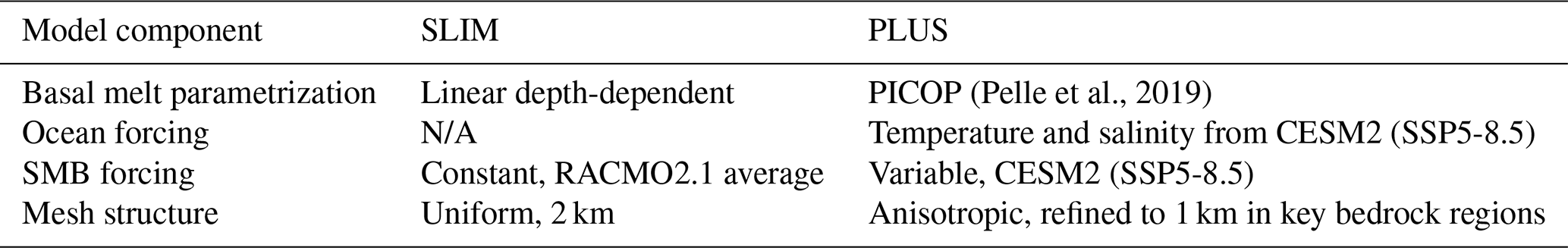
All simulations are performed using the Ice-sheet and Sea-level System Model (ISSM; Larour et al., 2012), which permits the coupling of an ice sheet model and a GRD model within a single consistent framework, with both models operating on the same grid. Ice sheet models are subject to a wide number of modeling choices, which can greatly affect the sensitivity of the coupled simulations. To check the robustness of our assessment of the sensitivity to resolution, we report our results for two widely different coupled model setups, labeled “Steady smb, Linear ocean melt, Isotropic Mesh” (SLIM) and “Picop ocean melt, Locally refined mesh, Unsteady Smb” (PLUS), which differ in the imposed surface mass balance (SMB), the basal melt parametrization, and the mesh type.

2.1 Ice sheet models

In SLIM, the ice sheet model uses a linearly depth-dependent ocean melt parametrization (Seroussi et al., 2014b) and a 2 km uniform mesh structure over ASE. Finally, a constant SMB forcing corresponding to the average between 1979 and 2010 from the Regional Climate Model RACMO2.1 is applied (Meijgaard et al., 2008). In PLUS, the ice sheet model features the cavity ocean melt model PICOP (Pelle et al., 2019), which captures the buoyant plume behavior of sub-shelf meltwater. Ocean temperature and salinity for PICOP are forced through 2300 using data from the Community Earth System Model 2 (CESM2) (Danabasoglu et al., 2020) for the Shared Socioeconomic Pathway (SSP), SSP5-8.5. PLUS also incorporates CESM2 SMB forcings through 2300 for the SSP5-8.5 scenario. From 2300 to 2350, SMB, ocean temperature, and salinity are held constant at their 2300 value. We use an anisotropic mesh structure in PLUS which sequentially progresses upstream of the initial grounding line. It is set to 1 km in areas with critical bedrock features, coarsens to 1.5–2 km in the grounding line retreat zone, and reaches 3.5 km in regions where moderate ice velocities (<250 m yr⁻¹) are simulated at the end of the simulation (see Appendix A1 for details). These differences between SLIM and PLUS are summarized in Table 1.

(Pelle et al., 2019)

Table 1 Summary of differences between the SLIM and PLUS models.

For both setups, we run simulations from 2000 to 2350 using the Shallow Shelf Approximation. To initialize the ice sheet geometry (ice surface, base, and bed topography), we use the BedMachine dataset (Morlighem, 2022) supplemented with Bedmap2 data (Fretwell et al., 2022). The SeaRise dataset (Le Brocq et al., 2010) is used for geothermal heat flow (Maule et al., 2005) and firn correction. The ice sheet model's time step is set conservatively to 2 weeks to capture rapid changes in the grounding line and ensure numerical stability. The grounding line is allowed to migrate such that ice starts floating if its thickness, H, is equal to or lower than the floating height H_f, defined as $H_{\mathrm{f}}=-\frac{{\mathit{\rho }}_{\mathrm{w}}}{{\mathit{\rho }}_{\mathrm{i}}}b,b<\mathrm{0}$, where ρ_i is the ice density, ρ_w is the water density, and b is the bedrock elevation. We use the sub-element parametrization SEP1 from Seroussi et al. (2014a) to track the grounding line position within mesh elements. No melt is applied to partially floating elements. Ice rheology and basal friction (${\mathit{\tau }}_{\mathrm{b}}=C_{\mathrm{b}}^{\mathrm{2}}{N}^r{v}_{\mathrm{b}}^s$; see Appendix A2 for details) are set to match initial velocities to observed velocities (Rignot et al., 2014). Although our study focuses on Thwaites Glacier and ASE, the mesh covers the entire globe. Annual ice mass changes for ice caps around the world are linearly extrapolated through 2350 based on GRACE-derived trends from 2003 to 2016 (Larour et al., 2017). This is notably to capture the initial global sea-level trend at the start of the simulation. While this contribution is minor compared to future West Antarctic mass loss at longer timescales, it ensures that any possible effect of present-day rising sea level on ASE's initial stability (Gomez et al., 2020) is accounted for. The background GIA signal from the Last Glacial Cycle (the response to ice and ocean loading between 122 kyr before present and the start of the Industrial Revolution) is also incorporated as an additional trend for the solid Earth and sea-level motion using the values provided by Caron et al. (2018). In line with Gregory et al. (2019), we use the terminology GRD for contemporary and future adjustments of the solid Earth and sea level, which are not included in the background GIA.

2.2 GRD model

The ice sheet model provides variations in ice loading to the GRD model at a regular time interval called the coupling interval. Accounting for rotational feedback, self-attraction, and the loading of the barystatic sea level (Adhikari et al., 2016), the GRD model computes the resulting changes in the bedrock and geoid. These updated fields are then fed back into the ice sheet model before it resumes its computations. For both SLIM and PLUS, the coupling interval is set to 1 year.

Following advances from Ivins et al. (2020, 2022, 2023), Lau (2023), and Faul and Jackson (2015), our rheology model supports transient mantle relaxation using the Extended Burgers Material (EBM). Transient rheologies have been shown to improve the fit of GIA models to relative sea-level indicators during meltwater pulse 1A while maintaining the performance of traditional Maxwell rheology models during periods of slower ice change (Simon et al., 2022; Lau, 2023). In a system coupling ice dynamics and solid Earth, including such rheology allows us to capture solid Earth feedback on decadal to centennial timescales. The EBM rheology includes the standard elasticity and steady-state viscosity parameters found in Maxwell models. In addition, transient relaxation is represented via an extra dissipative band bounded by periods τ_L and τ_H, with amplitude Δ, and frequency dependence controlled by a power-law parameter α, similar to attenuation laws in seismology (Ivins et al., 2020, 2023; Lau and Faul, 2019).

EBM rheology is used in mantle layers between the core–mantle and lithosphere–asthenosphere boundaries to compute viscoelastic Love numbers and derive the corresponding GRD patterns. This is achieved via the new GRD capabilities of ISSM (Adhikari et al., 2016; Larour et al., 2020, 2012; Farrell and Clark, 1976). In both SLIM and PLUS, GRD patterns are resolved at 1 km resolution (corresponding to a maximum Love number degree of 40 000).

The layers of the solid Earth model, in line with existing literature on regional mantle properties (Barletta et al., 2018), are described in Table 2. Although our model features a complete Earth structure down to the planet center in accordance with ISSM's Love number solver, we anticipate that the GRD response to mass changes in ASE is most sensitive to properties of the lithosphere and asthenosphere and comparatively less to the rest of the mantle (Barletta et al., 2018) given the spatial scale of loading considered. In comparison, signal originating from the ocean and ice loads in the far field is most sensitive to the deeper mantle (Caron and Ivins, 2020); thus our viscosity profile therein more closely aligns with global GIA models. The viscosities adopted in the asthenosphere fall on the lower end of values reported in the literature for ASE; hence the resulting feedbacks should be interpreted as an upper-bound scenario. Transient rheology (Caron et al., 2017) properties are set identically for all mantle layers below the lithosphere and are chosen in accordance with estimations given by Ivins et al. (2020, 2023) and Lau and Faul (2019), in which further description of the influence of each of these parameters is provided.

Table 2 Solid Earth parametrization. Density and shear modulus are taken from a volumetric average of the Preliminary Reference Earth Model (PREM; Dziewonski and Anderson, 1981) within each layer. The Earth model also includes a solid inner core and a fluid outer core layer with a density of 10 750 kg m³. Transient rheology properties include the relaxation strength parameter Δ, the power exponent α, and the low and high cutoff periods, τ_L and τ_H, delimiting the timescales in which the transient relaxation regime operates.

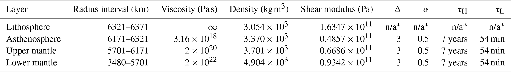
^* n/a: not applicable

3 Results

We firstly establish the baseline runs for both the SLIM and PLUS setups. We then expose in more detail the mechanisms by which GRD stabilization occurs. Finally, we assess the sensitivity of the grounding line retreat and GMSL contribution to the spatiotemporal resolutions tested.

3.1 Baseline viscoelastic runs for the SLIM and PLUS setups

We define baseline viscoelastic runs for both the SLIM and PLUS setups which serve as reference cases for our sensitivity study. Here, we examine the role played by GRD effects, mesh structure, basal melt parametrization, and SMB forcings in each setup. To quantify viscoelastic GRD stabilization induced by the transient EBM rheology described in the Methods section, we compare our baseline viscoelastic run to two additional runs: the uncoupled run in which no GRD effects are considered and the elastic run in which a solid Earth model with elastic compressible properties is employed. Figure 1 shows the position of the grounding line at year 2350 for these three runs for both SLIM (Fig. 1a) and PLUS (Fig. 1d) setups. Projections for two intermediary setups are also shown. The first is identical to SLIM except that the CESM2 SMB is used instead of the constant SMB (Fig. 1b). The second additionally includes PICOP and CESM2 ocean forcings in lieu of the linearly depth-dependent ocean melt parametrization (Fig. 1c). Across all setups, the inclusion of viscoelastic GRD effects reduces grounding line retreat by 30 to 200 km in 2350 (Fig. 1). Elastic stabilization plays a significant role in Fig. 1a and b, reducing grounding line retreat by 10–100 km. However, its effect is much weaker, with reductions of only 1–10 km, in Fig. 1c and d. Overall, we observe that GRD effects induce delay in the grounding line retreat but barely any change in the grounding line retreat pattern (additional visualizations are available in Appendix A3).

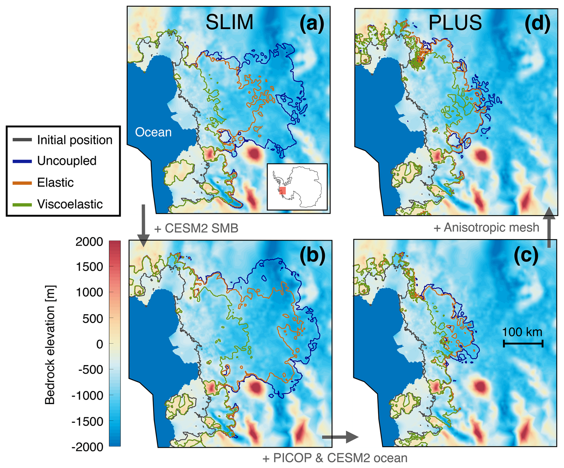
Figure 1 Grounding line projection in ASE at year 2350 for the SLIM (a) and PLUS (d) setups. Projections for intermediate setups are shown to illustrate the effects of incorporating CESM2 SMB forcings (b), PICOP with CESM2 ocean forcings (c), and an anisotropic mesh (d). The grounding line positions for the viscoelastic (green), elastic (brown), and uncoupled (blue) runs are overlaid on top of the bedrock topography. The initial grounding line position is represented in gray, and the ice-free ocean is depicted in solid blue. The location of the basin in Antarctica is shown in the bottom-right inset of panel (a).

In contrast, ocean melt, SMB, and mesh parametrizations affect not only the timing but also the pattern of the grounding line retreat. We observe a more extensive collapse in 2350 when including CESM2 SSP5-8.5 SMB instead of the constant-time SMB (Fig. 1a and b) used in SLIM. This is notably due to the negative CESM2 SMB values near Thwaites Glacier's grounding line from 2200 onwards. On the contrary, the use of PICOP with CESM2 ocean forcings leads to a less extensive collapse compared to linearly depth-dependent melt rate (Fig. 1b and c). Using an anisotropic mesh refined to 1 km in key regions instead of the 2 km uniform mesh induces a more extensive collapse (Fig. 1c and d).

Figure 2 presents the amplitude of elastic and viscoelastic bedrock uplift in 2350 for both the SLIM and PLUS setups. We observe 7.5 to 8.3 times more uplift in the viscoelastic runs compared to the elastic runs in the final year of our simulation (Fig. 2a–d). For a given run type, both setups exhibit similar uplift amplitudes and slight differences in uplift patterns.

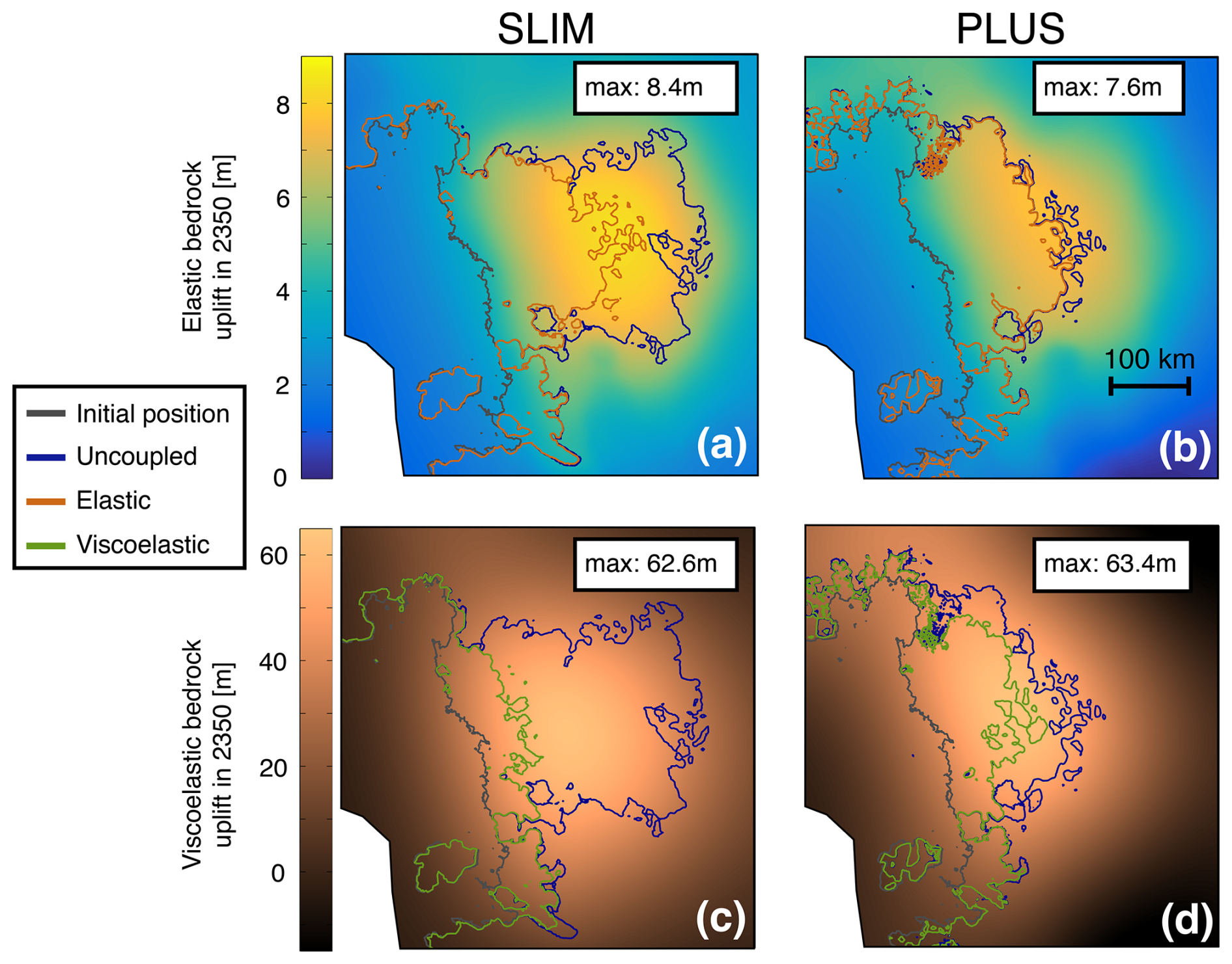
Figure 2 Bedrock uplifts at year 2350 for the SLIM (a, c) and PLUS (b, d) setups. The grounding line positions for the viscoelastic (green), elastic (brown), and uncoupled (blue) runs are overlaid on top of the elastic (a, b) and viscoelastic (c, d) bedrock uplifts. The initial grounding line position is represented in gray.

Figure 3 depicts the influence of GRD effects through time on Thwaites Glacier's GMSL contribution and ungrounded ice area for both SLIM (a–d) and PLUS (e–h) setups. The ungrounded ice area, which represents the ice surface transitioning from grounded to floating during the simulation, serves as a proxy for grounding line migration. This metric is particularly relevant as GRD effects primarily delay grounding line migration with only slight alterations to its retreat pattern. We note that Haynes Glacier is included in GMSL contribution and ungrounded ice area calculations, with additional details provided in Appendix A4. The GMSL contribution is computed in line with the method described in Adhikari et al. (2020). For SLIM, viscoelastic stabilization produces substantial negative feedbacks on Thwaites' ungrounded ice area (12.9 %) and GMSL contribution (5.6 %) by 2100 (Fig. 3b and d). These feedbacks reach 80.7 % and 53.1 %, respectively, by 2350. In PLUS, these feedbacks are slightly smaller but nonetheless considerable. Notably, Thwaites' contribution to GMSL is reduced by 13.9 % in 2200 and by 44.3 % by 2350 (Fig. 3f). By 2350, GRD effects induce a 47-year delay for the PLUS setup and a 125-year delay for the SLIM setup on the grounding line retreat (Fig. 3c and g).

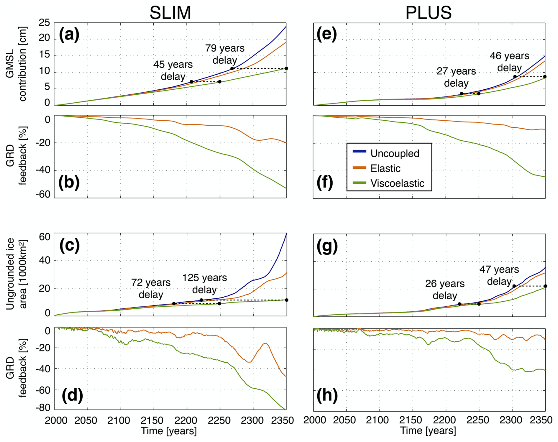
Figure 3 The evolution of Thwaites Glacier's GMSL contribution and ungrounded ice area in the SLIM (a–d) and PLUS (e–h) setups. GRD feedbacks represent the percentage reduction in GMSL contribution or ungrounded ice area resulting from including GRD effects. They are computed by comparing the results of the viscoelastic (green) and elastic (brown) runs with respect to the uncoupled (blue) run.

3.2 GRD effects prolong grounding line anchoring on bedrock ridges

For the viscoelastic and uncoupled runs of the PLUS setup, Fig. 4a shows the position of the grounding line in Thwaites' basin in the year 2292 overlaid on the bedrock elevation. Figure 4b and c depict the topography and the grounding line position, respectively, along the magenta flowline of Fig. 4a. We observe that the grounding line retreat evolves sporadically, alternating between short periods (∼1 year) of rapid retreat due to the retrograde bedrock slope and long periods (decades) of quasi-static anchoring on key bedrock features. A recent study highlighted the presence of two prominent ridges in the basin (Morlighem et al., 2020, Fig. 2a). The pink shadings (Fig. 4a–c) identify the first ridge that the grounding line reaches around 2100 in the PLUS setup. Here, we observe that the grounding line stays anchored 7 years longer in the viscoelastic run compared to the uncoupled run (Fig. 4c). The orange shadings identify the second ridge (Fig. 4a–c), which anchors the grounding line for 70 years in the uncoupled run and 100 years in the viscoelastic run (Fig. 4c). The cause of this difference in grounding line behavior is due to a larger bedrock uplift at the second ridge. This results from a larger ice mass change and a longer time period since the onset of ice mass loss, allowing more viscous deformation to accumulate.

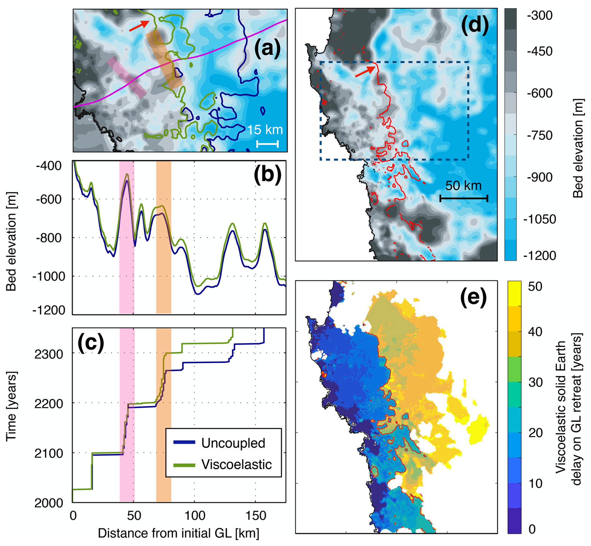
Figure 4 (a) Grounding line (GL) positions at year 2292 for the viscoelastic (green) and uncoupled (blue) runs of the PLUS setup overlaid on the initial bedrock. The initial GL is represented in black. (b) Topography along the magenta flowline. The green line includes viscoelastic uplift at year 2292. (c) GL migration (x axis) through time (y axis). The x axis is shared with panel (b). The pink and orange shadings indicate the locations of two key bedrock ridges which pin the GL for extended time periods. (d) Initial bedrock. The dotted blue box corresponds to the area depicted in panel (a). (e) Delay in GL retreat due to GRD effects. The red line identifies the 25-year delay isocontour which coincides with the second ridge of the basin and marks a sharp increase in the delay.

Figure 4d shows the topography over which the grounding line retreats in the viscoelastic run. Figure 4e represents the delay (number of years) separating the passage of the grounding line in the uncoupled and viscoelastic runs. In Fig. 4e, it is clear that an additional 20–30-year delay in the grounding line can be seen along the whole length of the second ridge, in agreement with results obtained through the study of individual flowlines (Fig. 4c) (Larour et al., 2019; Gomez et al., 2024). Another notable aspect of the interaction between the ice sheet and the solid Earth is highlighted by the constriction valley identified by the red arrow (Fig. 4a and d). Here, the grounding line stays pinned as well (Fig. 4a), despite low bed elevation due to the presence of the high lateral pinning points. This stabilization by “proximity pinning points” is also extended by ∼30 years (Fig. 4e) in the viscoelastic run.

3.3 Impact of model resolutions on grounding line position and GMSL contribution

This study focuses on three spatiotemporal resolutions: (i) the spatial resolution of the ice sheet model, (ii) the spatial resolution of the GRD response (controlled by the Love number degree in ISSM), and (iii) the coupling interval between the GRD model and the ice sheet model. These resolutions determine the computational cost and the accuracy at which the bedrock is resolved and updated throughout the simulations. Our goal is to determine the threshold values for these three resolutions that ensure the differences in GMSL contribution and ungrounded ice area remain under 5 % throughout the viscoelastic run, relative to the baseline viscoelastic run presented in Fig. 3 (green lines). Although a 5 % threshold is chosen for convenience in this study, we note that the practical acceptability of this error depends on the intended application and its importance relative to other sources of uncertainty. We focus on one parameter at a time, progressively varying it while keeping all other parameters at their baseline values. Overall, we find that, for both SLIM and PLUS, coarsening the resolutions invariably produces a qualitatively similar reduction in accuracy. As shown in Fig. 5, this effect is dominated by the ice sheet model resolution for short prediction horizons (2100), whereas the GRD resolution and the coupling time step become similarly important for longer horizons (2350).

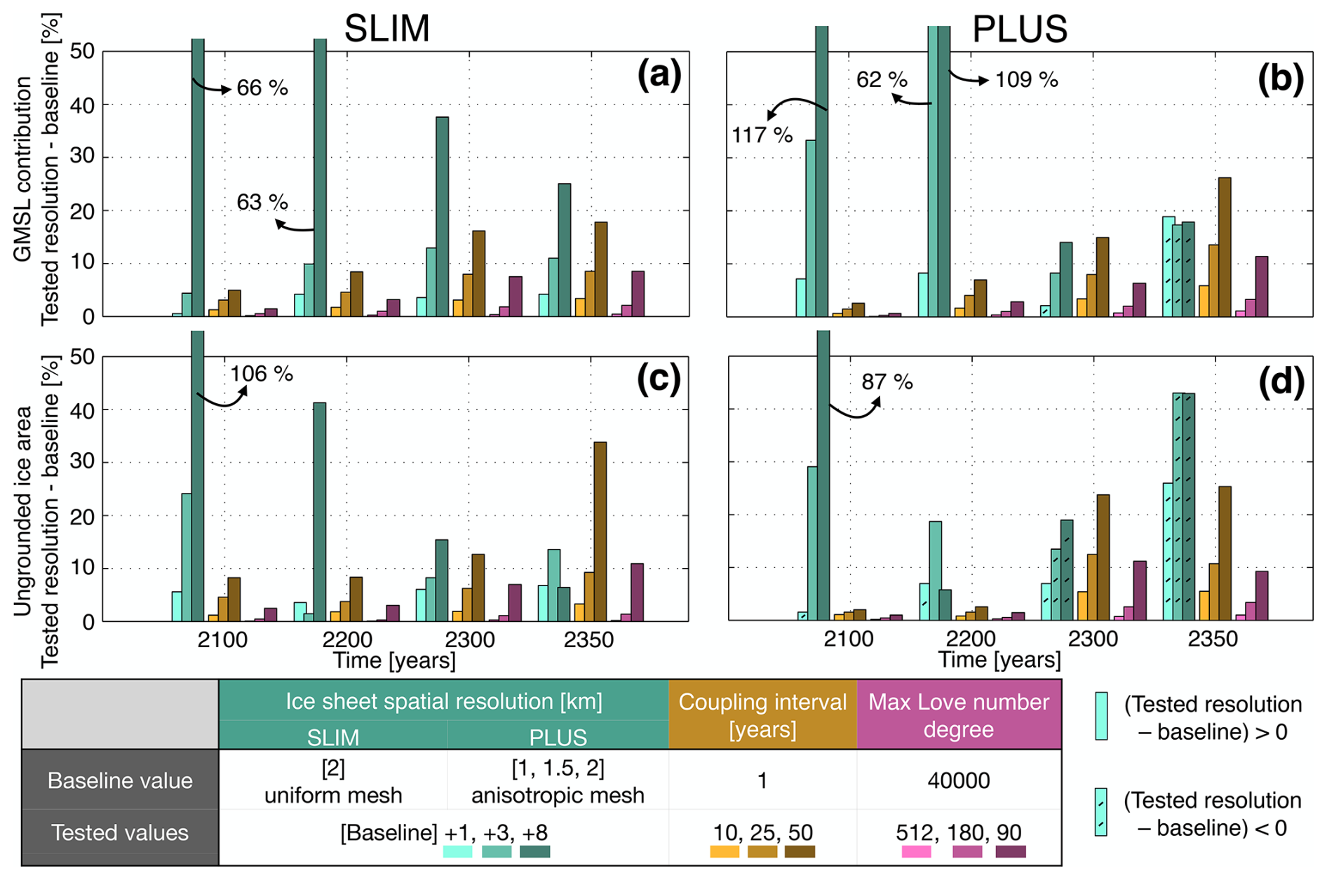
Figure 5 Sensitivity to (i) ice sheet spatial resolution, (ii) maximum Love number degree, and (iii) coupling interval for the SLIM (a, c) and PLUS (b, d) setups. For each tested resolution, differences to the baseline in GMSL contribution are represented in the top row and differences in ungrounded ice area are shown in the bottom row. Results are provided for four years (2100, 2200, 2300, 2350). For each parameter, three values are explored, with lighter colors indicating finer resolutions. For the ice sheet spatial resolution, the SLIM baseline uses a uniform 2 km mesh, while the PLUS baseline uses an anisotropic mesh refined to 1, 1.5, and 2 km in the region of grounding line retreat.

The ice sheet spatial resolution corresponds to the resolution at which both the ice sheet and the underlying bedrock are captured. We report the effects of coarsening the mesh by 1, 3, and 8 km. We keep the mesh structure unchanged for each setup. Hence, coarsening by 1 km means using a 3 km uniform mesh for SLIM. For PLUS, this means using an anisotropic mesh which progresses sequentially from 2–2.5–3 km in the grounding line retreat zone (Appendix A1). We observe a strong influence of the ice sheet spatial resolution through 2350. By 2100, coarsening by 1 km results in a 5.5 % increase in ungrounded ice area for SLIM (Fig. 5c) and a 7.1 % increase in GMSL contribution for PLUS (Fig. 5b), exceeding the 5 % threshold in both setups. This indicates that even the highest resolution used here has not fully converged. In the SLIM setup, GMSL contribution increases by 63 % for a 10 km mesh in 2200 and by 12.9 % for a 5 km mesh in 2300 (Fig. 5a). In PLUS, coarsening the mesh by 3 km reduces the ungrounded ice area by 42.9 % in 2350 (Fig. 5d). We note that the percent difference to the baseline sometimes decreases over time when using a coarser mesh (e.g., 10 km for SLIM), although the absolute difference increases.

The coupling interval is the number of years separating two GRD model computations which update the bedrock and sea-level positions. Using a 25-year coupling interval instead of the 1-year baseline leads to overestimating Thwaites Glacier's GMSL contribution in 2350 by 9.2 % in SLIM and 13.6 % in PLUS (Fig. 5a and b). In PLUS, a 10-year coupling interval induces over 5 % increase in both ungrounded ice area and GMSL contribution by 2350 (Fig. 5d). In line with previous studies (Book et al., 2022; Larour et al., 2019), we find that the coupling interval must be kept below 10 years (Fig. 5b and d) to satisfy our 5 % condition.

We define the spatial resolution of the GRD response as the minimum feature size that can be resolved by the GRD model. In ISSM, this is controlled by the maximum Love number degree, n, which is the spherical harmonic degree at which we truncate our Green's function series. The corresponding minimum wavelength that can be resolved, accounting for the limit to prevent aliasing, is given by $\mathit{\pi }\frac{R}{n}$, where R is the Earth's radius. Importantly, we note that this does not refer to the resolution at which the lateral variations in mantle rheology are resolved in 3D GRD models. We observe less than 1 % increase in GMSL contribution and ungrounded ice area for both the PLUS and SLIM setups when using n=512 (39 km) (Fig. 5a–d). However, with n=90 (222 km), the GMSL contribution increases by 8.5 % compared to the baseline in SLIM (Fig. 5a). We find that the solid Earth's response can be resolved at 111 km (n=180) and still verify the 5 % condition through 2350 in our GRD model.

4 Discussion

The results of this study indicate that the spatiotemporal resolutions of the ice sheet and GRD models can substantially impact projections of GMSL contributions and grounding line retreat. Here, we build on insights from analyzing coupled ice sheet and solid Earth interactions to explain this impact. We then discuss the implications of the observed GRD stabilization across model setups.

4.1 Resolution requirements can be explained by coupled model mechanisms

Keeping all other components of the coupled model identical, substituting the 2 km uniform mesh for the anisotropic mesh (1 to 2 km in the area of grounding line retreat) leads to substantially more collapse in 2350 (Fig. 1c and d). Although specific resolution requirements are model-dependent (Leguy et al., 2021), our results, in line with Williams et al. (2025), suggest that certain grounding line dynamics in this region can only be captured at kilometer-scale resolutions (Pattyn et al., 2013; Seroussi et al., 2014a; Seroussi and Morlighem, 2018; Robel et al., 2022). This outcome is also consistent with the kilometer-scale variations in the ridges and pinning points present in this area (Fig. 5a). A coarser mesh smooths out bedrock topography, potentially underestimating weaknesses in ridges such as bedrock lows between pinning points (red arrow in Fig. 4a). Conversely, this smoothing may lower stabilizing bedrock highs, thereby overestimating GMSL contribution (Fig. 5b). Here, we highlight a possible explanation for the large differences observed in ungrounded ice area (25.9 %) and GMSL contribution (18.8 %) when coarsening the mesh of the PLUS setup by 1 km (Fig. 5b and d). We anticipate that, in coupled simulations, spatial resolution of the ice sheet model is even more important. Firstly, it conditions the capture of fine features which are reinforced by viscoelastic uplift. Secondly, its high sensitivity means it has a large influence on the amount of unloaded ice which in turn conditions bedrock uplift. We note that, of the three resolutions studied, the ice sheet's spatial resolution is the only one that induces both increase and decrease in GMSL contribution and ungrounded ice area.

In PLUS, the increase in the ungrounded ice area remains small (<2.5 %) in 2100 and 2200 (Fig. 5d) for all coupling intervals considered. In 2300, a strong increase in ungrounded ice area (5.3 % for the 10-year interval and 12.5 % for the 25-year interval) can be seen. This can be explained by the fact that the grounding line breaks through the second ridge around 2290 (Fig. 4a). A similar effect can be observed in the 50-year interval simulation of the SLIM setup. In this case, the percent increase in ungrounded ice area rises sharply from 12.6 % in 2300 to 33.8 % in 2350 (Fig. 4c). The longer interval allows the grounding line to un-anchor from the second ridge, whereas the baseline model remains anchored through 2350 (see Appendix A5 for visualizations). We conclude that longer coupling intervals lead to faster collapse as more time is provided for ungrounding to happen prior to reinforcing key bedrock anchoring features. Results suggest that deformation on decadal timescales is significant enough to affect the floatability threshold. This is consistent with the relaxation timescales under 7 years included in our transient mantle rheology model.

A lower maximum Love number degree means that GRD deformation is applied more diffusely. For PLUS, setting n=90 results in over 12 % less uplift (see Appendix A6 for details) in the vicinity of key bedrock features compared to the baseline, causing a 11.3 % increase in GMSL contribution by the final year of the simulation (Fig. 5b). For both setups, we find that the maximum Love number degree can be set to n=180 (111 km) and entail under 3.3 % differences to the baseline (Fig. 5a–d). This suggests that the solid Earth response to Thwaites' mass loss is dominated by relatively large wavelengths on the order of the size of Thwaites' basin (Fig. 2c and d) even when the Love numbers allow responses on much smaller scales (∼1 km). In turn, this implies significant ice thickness changes on scales of 100 to 300 km (Appendix A7). The resolution requirements identified here differ from previous estimates by Wan et al. (2022), who found bedrock deformation and geoid motions to converge within 5 % for spatial resolutions of 7.5 km or higher in their GRD model. However, they reported that this threshold was influenced by short-wavelength ice mass loss patterns during the first 25 years of their simulation, which later transitioned to being dominated by longer-wavelength patterns. Some discrepancy may also arise from differences in the GRD models. For instance, their model uses grid-based GRD computations and incorporates lateral variations in rheology, whereas our model employs a Love number solver and accounts for transient mantle rheology. Finally, the metric used to determine convergence differs between the two studies. We emphasize that, in this study, the spatial resolution of the GRD response refers to the smallest variations in ice and ocean loading that can be resolved by the GRD model. It is distinct from the resolution used to capture variations in mantle viscosity in 3D GRD models.

This sensitivity study is focused on Thwaites Glacier due to the low viscosity observed in West Antarctica and the importance of this glacier for future sea-level projections. We expect studies focused on other basins to obtain qualitatively similar results with varying numbers from those presented here, as they depend on basin topography and mass change patterns. Additionally, we expect these numbers to vary based on the metrics used to determine convergence. To illustrate, the integrated metrics used in this study, such as GMSL contribution and ungrounded ice area, are well suited for studies focused on sea-level projections. However, these metrics may be less adapted for investigations focused on more localized variables, such as vertical displacement from GPS stations (Kachuck et al., 2020). In such cases, convergence based on bedrock deformation is more relevant (Lucas et al., 2025).

Nevertheless, this study follows a reproducible framework for analyzing the individual influences of various modeling choices which can easily be applied to other convergence metrics, basins, and modeling choices. Notably, it will be useful to extend this work to ice rheology, basal friction (Berdahl et al., 2023), and mantle rheological properties whose influences have not been explored in this study.

4.2 Implications of GRD stabilization across different coupled models

In this study, we investigate coupled ice sheet–GRD models and observe important viscoelastic stabilization across widely different model setups (Figs. 1 and 3). We conclude that, in high-resolution simulations of West Antarctica, independently of other model components (mesh structure, ocean melt, SMB), rapid viscoelastic stabilization cannot be ignored. Indeed, uncoupled models risk overestimating Thwaites' contribution to GMSL by 5.6 % in 2100 (Fig. 3b) and over 30 % in 2300 (Fig. 3f). Our findings revisit prior conclusions based on ISSM (Larour et al., 2019) by incorporating viscous GRD effects using transient EBM rheology. They also complement previous studies that focused primarily on mantle rheology (Book et al., 2022; Gomez et al., 2024), confirming the need to include coupled ice sheet–GRD models in future projection frameworks.

In choosing only one set of mantle rheological properties, we acknowledge that we are not exploring the uncertainty affecting the solid Earth structure. Hence, the results presented do not constitute definitive predictions of the state of the ice sheet or the strength of GRD feedback. Rather, our focus lies in determining the spatiotemporal-resolution requirement of coupled models for a given solid Earth parametrization that exhibits the decadal to centennial response required to explain current vertical land motion data in the region (Barletta et al., 2018). A fast yet realistic parametrization of the viscoelastic uplift is deliberately used here to study resolution sensitivity under a “high-deformation scenario”. Hence, the requirements identified for coupling interval and spatial resolution of the GRD response are likely conservative estimates and should apply to less aggressive parametrization as well. This approach is particularly relevant given the large uncertainty in West Antarctica's mantle rheology (Ivins et al., 2023).

This uncertainty in mantle rheology underscores the importance of ongoing investigations of 3D GRD models (Gomez et al., 2024). While our GRD model does not include lateral variations in mantle rheology, we expect similar conclusions for the resolutions studied here in coupled simulations using 3D GRD models given similar GRD feedbacks. Should GRD effects be weaker, we would expect resolution requirements identified here on coupling interval and spatial resolution of the GRD response to be relaxed. Here, we highlight an opportunity for future studies using coupled models with 3D mantle rheology to investigate the distinct influences of (i) the ice sheet spatial resolution, (ii) the spatial resolution of GRD response, (iii) the coupling interval, and (iv) the spatial resolution of lateral variations in the solid Earth building on work by (Wan et al., 2022). We note that novel methods (Swierczek-Jereczek et al., 2024) must be further investigated to address the high computational cost associated with coupled models that incorporate 3D mantle rheology. We anticipate that studies focusing on computationally expensive ice sheet dynamics (Pattyn et al., 2008; Favier et al., 2012) which seek to incorporate GRD effects will need to find compromises between the computational cost and complexity of GRD models. This is especially true when considering uncertainty quantification efforts which require large ensembles of model runs.

5 Conclusions

We simulate the collapse of Thwaites Glacier through 2350, taking into account coupled ice sheet, solid Earth, and sea-level interactions. We investigate the sensitivity of the coupled model to (i) the mesh resolution of the ice sheet model, (ii) the spatial resolution of the GRD response, and (iii) the coupling interval between the ice sheet model and the GRD model. Results indicate that coarsening a kilometer-scale ice sheet mesh by 1 km leads to significant changes in the projected GMSL contribution, with differences reaching 7.1 % in 2100 and 18.8 % in 2350. We find that both GMSL contribution and ungrounded ice area converge within 3.3 % through 2350 for maximum Love number degrees above 180. Further investigation is needed to determine whether GIA models accounting for lateral viscosity variation are typically more sensitive to higher mesh resolution in conditions comparable to our simulations. In particular, this sensitivity may depend on the resolution of the input seismic tomography model in the lithosphere and sublithospheric mantle structure. This study also shows that decadal to sub-decadal coupling intervals are necessary to capture the full stabilizing effect of bedrock uplift.

Our findings point to an increasingly recurrent dilemma facing modelers who must ensure computational feasibility and cost without forgoing the capture of mechanisms which can only be resolved at high spatiotemporal resolutions. Indeed, high spatial resolution of the ice sheet, including bedrock topography, and short coupling intervals comes at heavy computational cost. Notably, continental-scale simulations are not compatible with the high resolution of local basin-scale studies. Further investigations of alternative GRD computational methods (Swierczek-Jereczek et al., 2024), mesh refinement techniques (Larour et al., 2012; Hecht, 1998; dos Santos et al., 2019), and other model optimizations (Han et al., 2022; van Calcar et al., 2023) are needed to solve this issue.

This study also highlights the crucial role played by pinning points and ridges in coupled simulations of ASE. We observe that modeled grounding line retreat alternates between phases of rapid migration between sets of laterally extending ridges and long quasi-static phases on these ridges. We find that viscoelastic adjustment could anchor the grounding line on these key bedrock features an additional 30 to 125 years. We expose this mechanism as a major driver of the enhanced stability observed in coupled simulations of marine ice sheets. Given the importance of this mechanism and the current uncertainty in bed topography (Morlighem et al., 2020), we emphasize the crucial need for ongoing and future bedrock measurements to better constrain the topography of subglacial ridges.

Appendix A

A1 Anisotropic mesh parametrization of the PLUS setup

The grid remains fixed over time in both SLIM and PLUS. Most of the grounding line retreat through 2300 occurs in the 1 km mesh area (light blue) for the viscoelastic baseline run in PLUS. This is evidenced by the grounding line position at year 2300 (bright purple). For reference, the ASE region illustrated in Fig. A1b includes the Pine Island, Thwaites, Smith, Pope, Kohler, and Haynes glaciers.

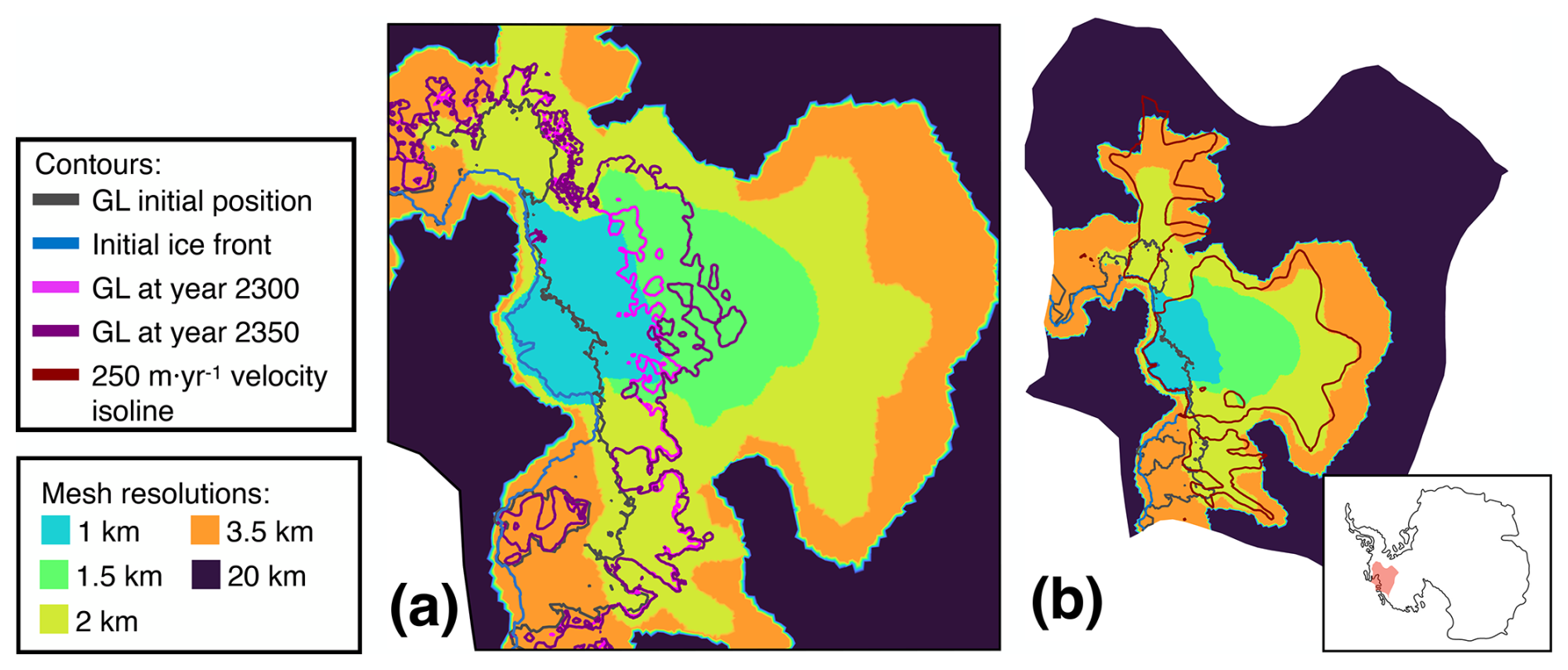
Figure A1 Illustration of the different areas of the PLUS anisotropic mesh with distinct mesh resolutions. Baseline resolution values are indicated in the legend. Panel (a) depicts the region shown in Figs. 1 and 2. The grounding line position at years 2300 and 2350 from the viscoelastic run are overlaid for reference. Panel (b) shows the broader region of ASE on which this study focuses. The dark-red contour represents the 250 m yr⁻¹ ice velocity isoline. In panel (a) and panel (b), initial grounding line and ice front positions are shown in gray and blue, respectively. The bottom-right inset shows the location of panel (b) within Antarctica.

A2 Further details on model initialization

The friction law is implemented in terms of basal stress: ${\mathit{\tau }}_{\mathrm{b}}=C_{\mathrm{b}}^{\mathrm{2}}{N}^r{v}_{\mathrm{b}}^s$. The friction coefficient C_b field is set such that initial velocities are optimized to observed velocities. N is the effective pressure, and v_B is the basal velocity magnitude. r and s are the friction law exponents which are both set to 1 in our model. Figure A2 shows (a) the observed velocity in ASE, (b) the initial velocity determined after friction and rheology optimization, and (c) the absolute difference between the observed and initial velocities. The friction and rheology parameters are optimized separately for the SLIM and PLUS setups. For all experiments (e.g., uncoupled/elastic/viscoelastic runs and varying resolutions) within a given setup, we use the same optimized friction and rheology fields. This is to permit a parametric study in which only the resolution (or solid Earth parametrization) under study is varied, while all other model resolutions and parameters are held constant.

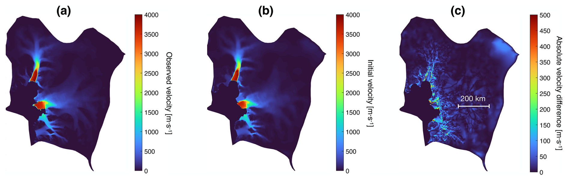
Figure A2 Velocity in ASE in the PLUS setup: (a) observed velocity, (b) initial velocity (simulated after optimization of friction and rheology), and (c) the difference between the observed and initial velocities.

A3 GRD effects induce delay on grounding line retreat but barely any retreat pattern change

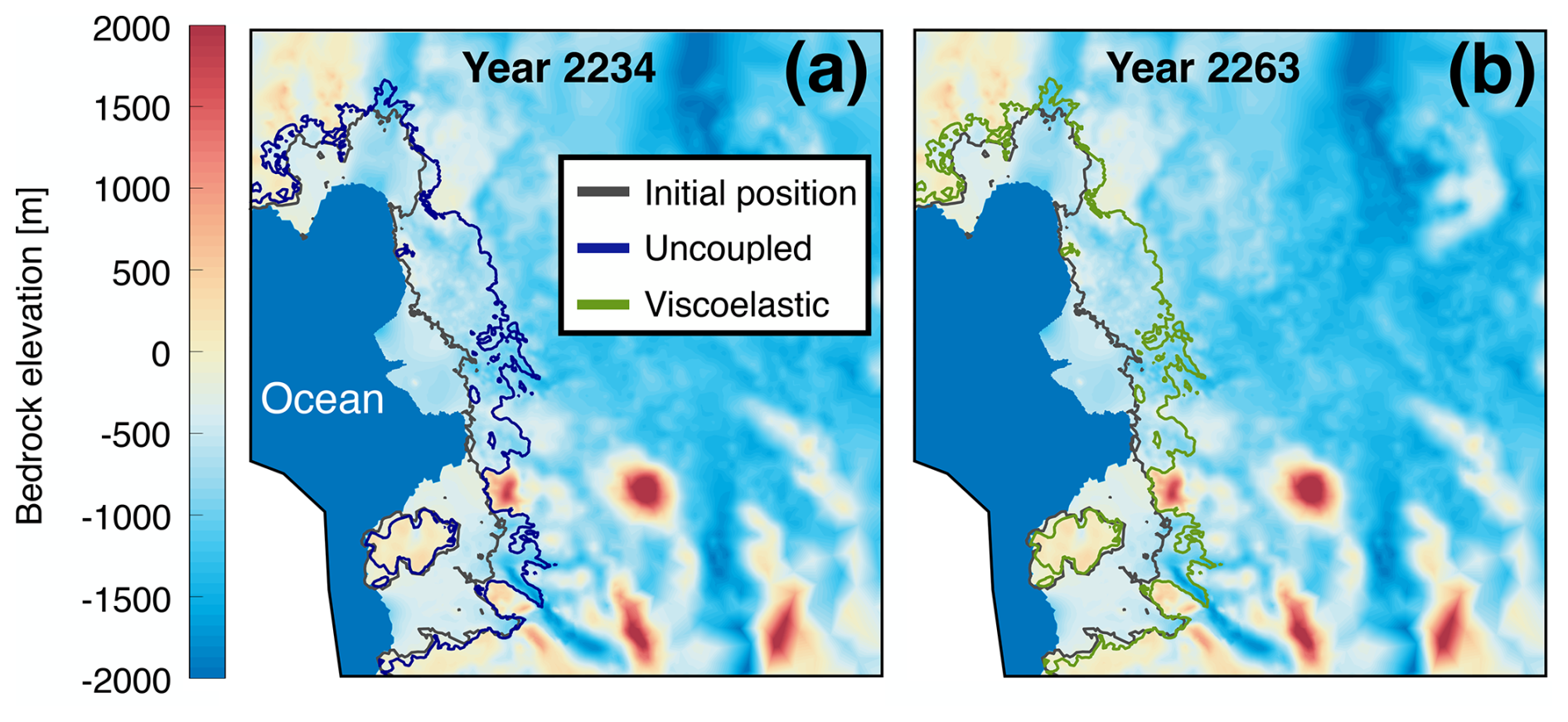
Figure A3 Grounding line projections in ASE in the PLUS setup. (a) Projection for the year 2234 in the uncoupled run (blue). (b) Projection at year 2263 in the viscoelastic run (green). The initial grounding line position is shown in gray.

A4 Calculation details for GMSL contribution and ungrounded ice area

The brown contour shown in Fig. A4 defines the region used to compute the GMSL contribution and ungrounded ice area. While it does not strictly follow a classical drainage basin definition, it approximately encompasses the Thwaites and Haynes glacier basins. The region was intentionally extended to include areas where significant divergence in grounding line position develops between the viscoelastic and uncoupled simulations by 2350. This extension ensures that the full spatial extent of the GRD feedback is accounted for in calculations of GMSL contribution and ungrounding ice area.

Furthermore, we note that, in coupled models, the classic “height above floatation (HAF)” method to calculate GMSL contribution is flawed due to bedrock and geoid motion. Hence, we apply the methodology developed by Adhikari et al. (2020) for our GMSL contribution calculations.

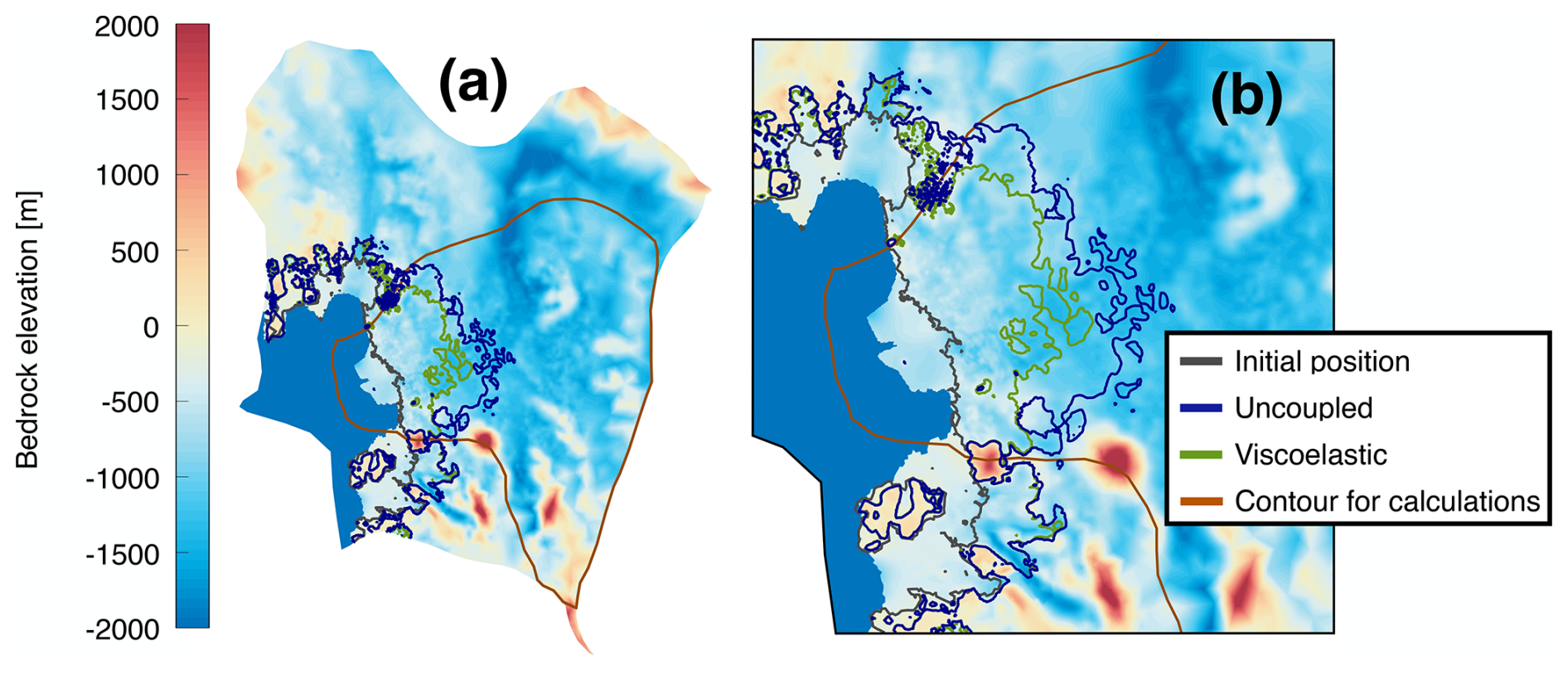
Figure A4 Contour of the region over which GMSL contribution and ungrounded ice area are calculated throughout the paper (brown). Viscoelastic (green) and uncoupled (blue) grounding line projections in 2350 for the PLUS setup are overlaid for reference. The initial grounding line position is shown in gray. Panel (a) represents the region of ASE under study, and panel (b) corresponds to the region depicted in Figs. 1 and 2.

A5 Increasing the coupling interval to 50 years causes the grounding line to un-anchor from the second ridge before 2350 in SLIM

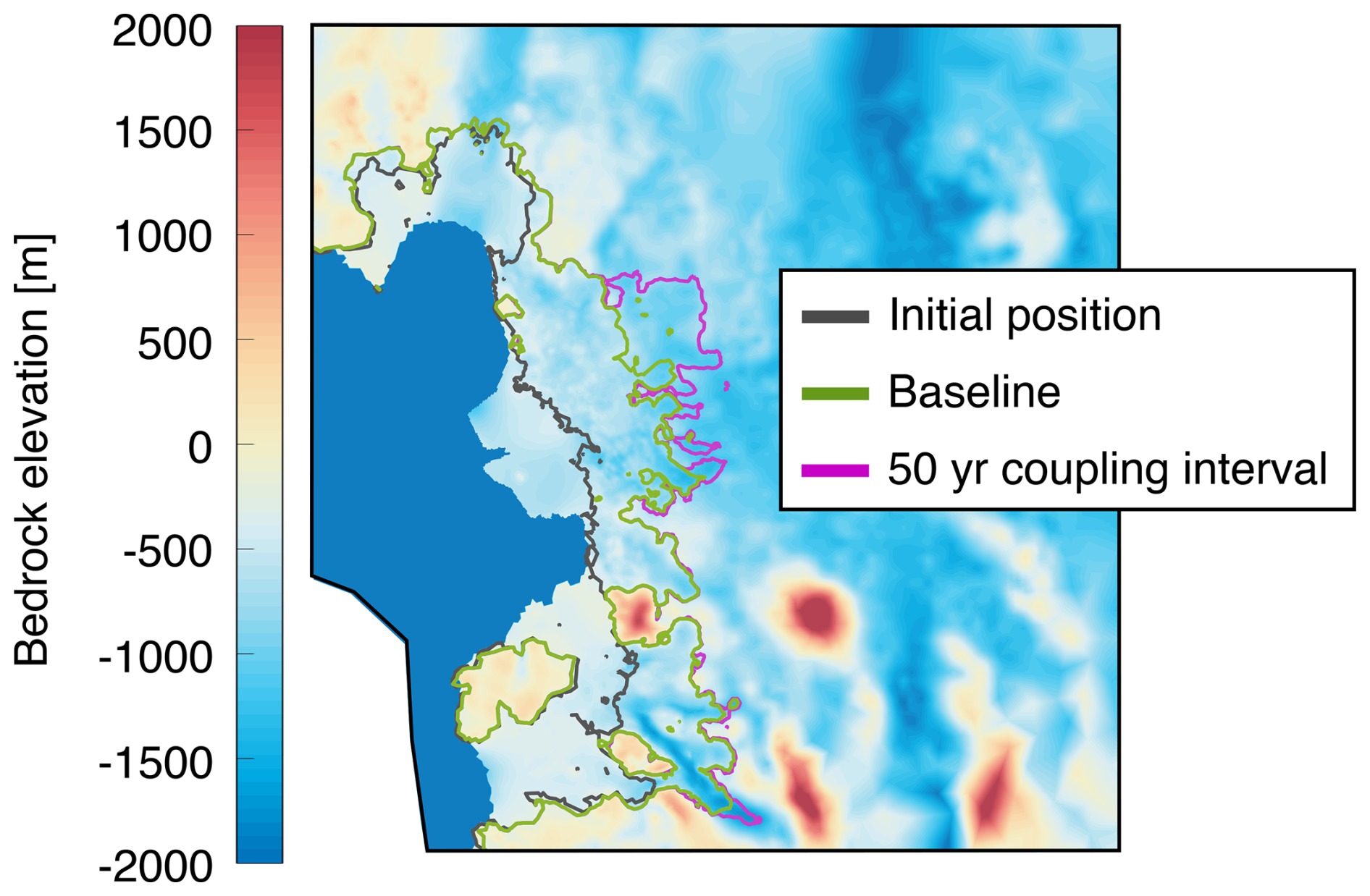
Figure A5 Grounding line projections in the SLIM setup at year 2350. The projection for the baseline viscoelastic run (green) is shown alongside the projection for the 50-year coupling interval run (magenta). The initial grounding line position is shown in gray.

A6 Decreasing the maximum Love number degree reduces bedrock uplift in the grounding line retreat zone

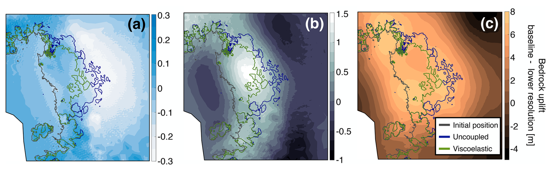
Figure A6 Loss in bedrock uplift due to setting the maximum Love number degree in the PLUS setup to (a) 512 (39 km), (b) 180 (111 km), and (c) 90 (222 km) instead of the reference value of 40 000 (1 km). Grounding line positions at year 2350 for the viscoelastic (green) and uncoupled (blue) runs are overlaid for reference. The initial grounding line position is shown in gray. Note that the color bar scales vary between panels.

A7 Grounded ice thickness change patterns are on the order of hundreds of kilometers

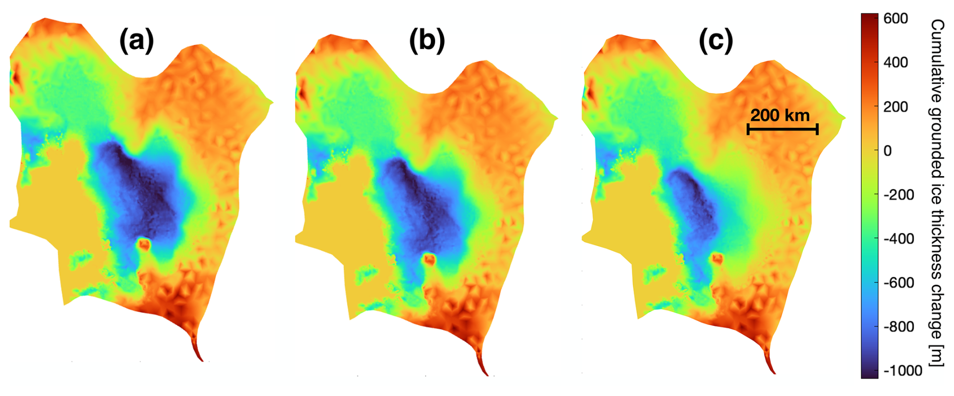
Figure A7 Cumulative grounded ice thickness change through 2350 in the (a) uncoupled, (b) elastic, and (c) viscoelastic runs of the PLUS setup.