Retrieval of atmospheric water vapor and temperature profiles over Antarctica from satellite microwave observations using an iterative approach

Retrieving atmospheric water vapor and temperature profiles over land using microwave radiometry is challenging due to uncertainties in estimating surface emissions. To address this, we developed an approach that couples the atmospheric retrieval algorithm with the surface emission estimation in an iterative loop. Using sounding channels from Ka- to G-band on the Advanced Technology Microwave Sounder (ATMS), we retrieved temperature and humidity profiles across the Antarctic region throughout the year 2016. The atmospheric profiles are updated in each iteration and used in the following step to refine the surface emissivity. This process continues until the atmospheric solution converges. The main innovation is the integration of surface and atmospheric retrievals, which improves overall accuracy. We validated our results against in situ radiosonde data. The algorithm accurately retrieved temperature profiles, along with surface emissivity across 23–165 GHz, and successfully detected ice sheet meltings. While it captured water vapor variability, accurate absolute humidity values still require an independent surface emissivity retrieval using additional observations.

1 Introduction

The Greenland and Antarctica ice sheets are major contributors to global sea level rise due to increasing ice melt (Rignot et al., 2011). This highlights the need to monitor and understand the mechanisms driving the accelerated melt events (Noble et al., 2020). Effectively monitoring and analyzing the ice sheets require a detailed understanding of the atmospheric conditions that influence these regions (Le clec'h et al., 2019), which is also essential for predicting the future evolution of ice masses (Le clec'h et al., 2019). Current atmospheric temperature and humidity retrievals in the microwave spectral range face challenges, primarily due to uncertainties in estimating surface emission. These challenges are amplified over polar ice sheets, where the atmosphere is typically dry, the surface emissivity changes rapidly during melt seasons, and the background emission is relatively high (Miao et al., 2001). Traditional retrievals are limited by the absence of direct surface emissivity measurements and uncertainties in modeling background emission. To overcome these issues, we implement an iterative strategy that couples atmospheric retrieval with surface emission estimation. This approach enhances the accuracy of retrieved atmospheric temperature and humidity profiles, supporting improved understanding of the processes that drive melt in the Greenland and Antarctic ice sheets.

The Advanced Technology Microwave Sounder (ATMS), on board polar-orbiting satellites, is designed to perform atmospheric temperature and humidity sounding through oxygen and water vapor absorption bands (Goldberg and Weng, 2006; Muth et al., 2005). We applied our iterative retrieval algorithm to ATMS data across Antarctica during 2016. This year was selected due to the significant melt anomaly over Ross Ice Shelf during 2016 austral summer (e.g., Nicolas et al., 2017; Mousavi et al., 2022; de Roda Husman et al., 2024; Hansen et al., 2024), which provided ideal conditions to assess the impact of varying surface emissivity on atmospheric retrievals. This analysis enabled us to evaluate the performance and limitations of the iterative approach.

2 Observations

2.1 Observation data – ATMS data

The satellite carrying ATMS follows a sun-synchronous polar orbit, completing about 14 orbits per day and enabling frequent revisit opportunities, especially at high latitudes. Over the Antarctic region, this results in 4 to 10 ATMS overpasses per day for any fixed location, with variations due to swath width (∼ 2500 km), scan angle geometry, and Earth rotation. ATMS has 22 channels to receive and measure radiation from different layers of the atmosphere, obtaining global data on tropospheric humidity and temperature at either quasi-vertical or quasi-horizontal polarization. Table 1 summarizes the radiometric characteristics of the ATMS channels, while Fig. 1 shows their spectral positions relative to atmospheric opacity from oxygen and water vapor absorption. ATMS channels cover the oxygen band (50–58 GHz), the two water vapor lines at 22 and 183 GHz, and several window channels (see Fig. 1). The temperature information of the atmosphere is obtained from Channels 3 to 15. Channels 18–22 are centered at the 183.31 GHz water vapor line but with a successively narrower bandwidth from ±7 to ±1 GHz, giving humidity information on successively higher troposphere.

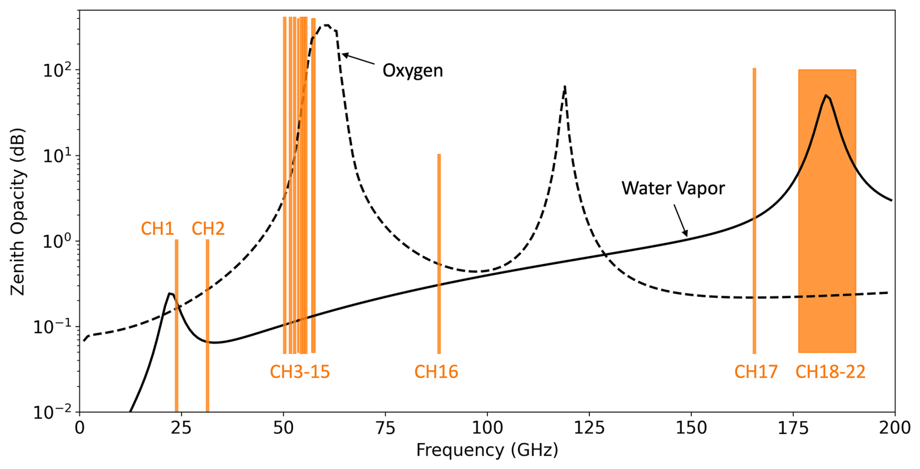
Figure 1 Spectra positions of 22 ATMS channels, on top of zenith opacity from oxygen and water vapor.

Table 1 Key characteristics of the 22 ATMS channels.

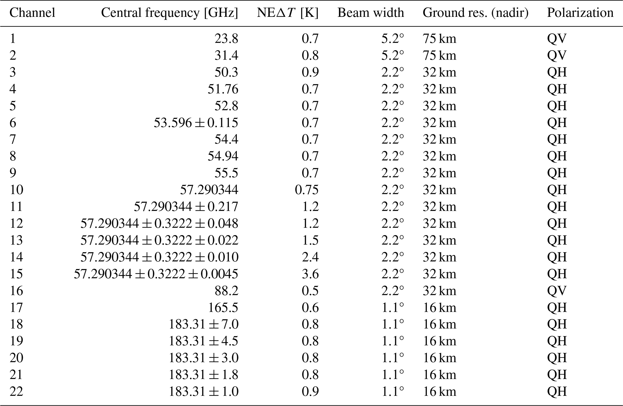
Figure 1 shows the zenith opacity of a typical polar dry atmosphere for the ATMS frequency range. The opacity is dominantly caused by water vapor and oxygen in the atmosphere. The contribution of nitrogen, orders of magnitude smaller and without any spectral line at this frequency range, can be neglected. The total opacity is computed by integrating the opacity per unit length from the top of the atmosphere toward the surface (Meeks and Lilley, 1963). Channels 1, 2, 16, and 17 are located at transparent window regions, where the opacity is low. Jacobians of temperature and water vapor channels typically peak near the maximum of the weighting function, which often corresponds approximately to the atmospheric level where the optical depth is near unity (Petty, 2006). For the window channels, the overall opacity is much less than one. These channels can see through the atmosphere and are sensitive to Earth's surface emission; therefore, they can be used for deriving surface emissivity. However, at oxygen (58 GHz) and water vapor (183 GHz) absorption bands, the observed brightness temperature is not very sensitive to the surface emission. The surface emissivity at these frequencies will be derived using the adjacent channels that have relatively low opacity: CH3 (50.3 GHz) will be used to derive the emissivity in the range of 50.3–57.29 GHz (CH3 to CH15) at QH polarization; CH18 (183.31 ± 7 GHz) for the emissivity near 183.31 GHz (CH18 to CH22) at QH polarization. In all, we derive surface emissivity for the window channels 1 (23.8 GHz), 2 (31.4 GHz), 3 (50.3 GHz), 16 (88.2 GHz), 17 (165.5 GHz), and 18 (183.31 ± 7 GHz) and assume linear emissivity variation between these frequencies.

The beam width of ATMS varies with frequency: 1.1° for channels in the 160–183 GHz range, 2.2° for the 50–60 and 80 GHz channels, and 5.2° for the 23.8 and 31.4 GHz channels (Kim et al., 2014, 2020). Both SNPP (Suomi National Polar-orbiting Partnership) and the NOAA-20 (National Oceanic and Atmospheric Administration 20, also known as Joint Polar Satellite System 1, JPSS-1) satellites orbit at an altitude of approximately 830 km. This results in instantaneous spatial resolutions on the ground at nadir of about 16, 32, or 75 km, depending on the channels. Due to the cross-track scanning approach, the instrument provides observations at a wide range of incidence (off-nadir) angles. To ensure accuracy, we include only observations with an incidence angle less than 60°, as the instrument footprint increases approximately with $\mathrm{1}/$(cos²θ). For each fixed reference location, we use only those ATMS observations whose beam boresight lies within 22.24 km (corresponding to 0.2° angular separation), ensuring spatial relevance. The ATMS data used in this work were obtained from the Comprehensive Large Array-data Stewardship System (CLASS) of NOAA.

To better understand the vertical sensitivity of each ATMS channel to atmospheric temperature and water vapor, we examine the Jacobians, which describe how changes in these variables influence observed brightness temperature. Figure 2 shows the temperature (upper right) and water vapor (lower right) Jacobians at all 22 ATMS channels for December (austral summer) atmospheres, representative of Antarctica conditions. The Jacobians are calculated by increasing the water vapor and temperature at each vertical layer to the orange dashed line, using the same 73-layer vertical grid as MERRA profiles (see Sect. 2.2), ranging from two meters above the surface to over 70 km in altitude. Therefore, a positive value implies that adding water vapor or increasing temperature will increase the radiance observed by the instrument and vice versa. The Jacobian shows the sensitive altitudes of each channel. Near the oxygen absorption band, CH3 to CH15 are sensitive to successively higher altitudes, up to ∼ 60 km above the sea level. Channels 18–22 are located near the water vapor line at 183.31 GHz. The atmospheric opacity for these channels differs significantly, making these channels sensitive to different layers of the atmosphere. The bandwidth of these channels decreases with the channel number, with Channel 22 being the narrowest and Channel 18 being the broadest. The water vapor Jacobians for Channels 18–22 indicate sensitivity to distinct atmosphere layers extending up to several kilometers above the surface. Above approximately 10 km, the atmospheric water vapor content is so low that typical perturbations fall below the detection threshold of ATMS. The Jacobians shown are from the nadir view (0° incidence angle). Jacobians corresponding to off-nadir angles peak at slightly higher altitudes due to the longer atmospheric path length traversed by the radiation.

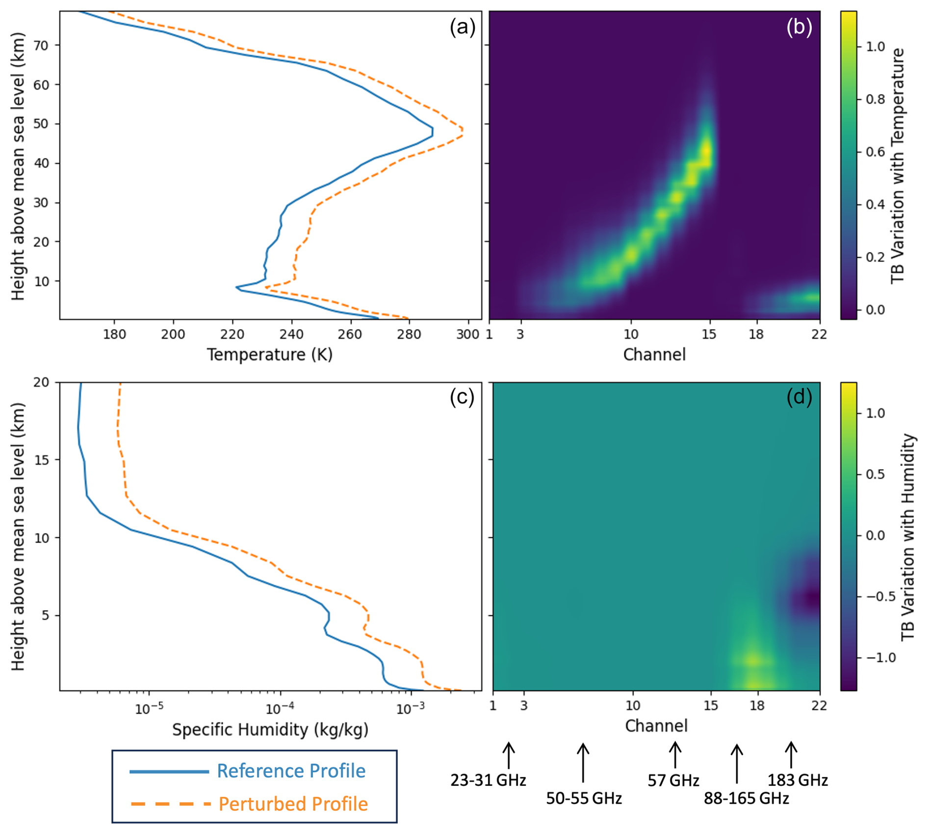
Figure 2 Typical Antarctica atmospheres for summer (December) weathers at WAIS DIVIDE (79.5° S, 112° W). The plots show the temperature profile (a) and the specific humidity profile (c), the temperature Jacobian (b), and the water vapor Jacobian (d) for all 22 ATMS channels. The Jacobians are based on nadir view (0° incidence angle).

2.2 The prior – MERRA-2

Using ATMS microwave thermal emission measurements, we applied optimal estimation (OE) to retrieve the atmospheric temperature and humidity profiles. OE, as outlined by Maahn et al. (2020), is a widely used physical retrieval method that incorporates measurements, prior information, and their uncertainties. Based on Bayes' theorem, OE estimates the most probable atmospheric state. Prior information plays a critical role in the retrieval process. We use the Modern-Era Retrospective analysis for Research and Applications, version 2 (MERRA-2), as the prior for temperature and water vapor profiles. We use the “tavg3_3d_asm_Nv” dataset, which offers 3-hourly averaged atmospheric profiles across 72 hybrid sigma-pressure levels (Rienecker et al., 2008), with a spatial resolution of 0.625° longitude by 0.5° latitude. For ice and liquid water cloud distributions, we used the MERRA-2 three-dimensional cloud fields, which provide vertically and horizontally resolved profiles of cloud water and ice content. To account for surface characteristics such as skin temperature, temperature/humidity/wind speed at 2 m, and surface pressure, we integrated MERRA-2 single-level diagnostics data labeled as “tavg1_2d_slv_Nx”. By merging the three-dimensional assimilated meteorological data with the single-level diagnostics data, our analysis extends across 73 vertical layers starting from two meters above the surface and extending beyond 70 km into the atmosphere. The vertical grid is close to equidistant in the logarithm of the pressure and approximately equidistant in altitude.

To illustrate the structure and seasonal variability of the a priori profiles used in the retrievals, Fig. 3 presents the seasonal mean temperature and specific humidity profiles from MERRA-2 at three representative Antarctic sites: McMurdo Station, the South Pole, and the Antarctic Peninsula. These locations span different climate regimes, and the profiles exhibit clear seasonal contrasts – especially the colder, drier winter atmosphere and the distinctive temperature inversions near the tropopause. This spatial and temporal variability highlights the importance of location- and season-specific a priori knowledge in OE retrievals. It is also important to note that the MERRA-2 priors are provided with respect to height above mean sea level, and the surface elevation differences among the selected sites (e.g., higher elevation at the South Pole vs. coastal McMurdo) are preserved in the a priori structure. This ensures that retrievals remain physically consistent with the local topography and atmospheric structure. In addition to the mean state profiles, the OE algorithm also incorporates the a priori error covariance matrix, which encodes the expected variability and vertical correlation of atmospheric parameters. It plays a critical role in weighting the influence of the prior relative to the measurements and governs the vertical smoothing and retrieval precision.

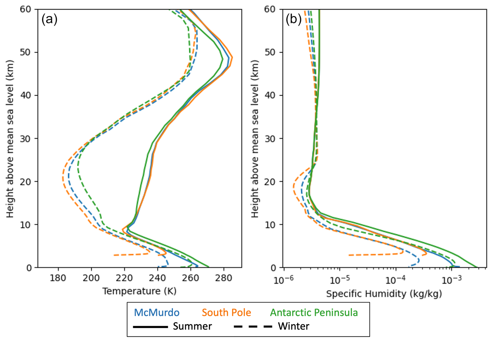
Figure 3 Seasonal average profiles of temperature (a) and specific humidity (b) from MERRA-2 for three representative Antarctic locations: McMurdo Station, the South Pole, and the Antarctic Peninsula. Solid lines represent summer; dashed lines represent winter. These profiles are used as a priori inputs in the retrieval algorithm and illustrate regional and seasonal variability in atmospheric conditions.

2.3 In situ and ground-based remote sensing observations

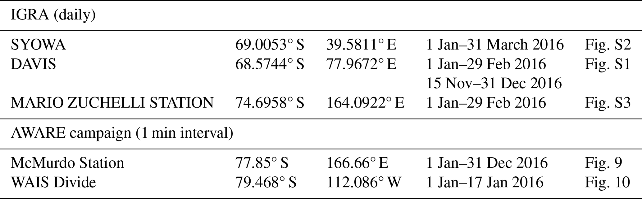
Across Antarctica, a network of radiosonde stations provides in situ measurements of atmospheric profiles. These stations contribute to the Integrated Global Radiosonde Archive (IGRA), which provides valuable long-term in situ measurements, though often at limited temporal resolution depending on station operations (Durre et al., 2006). However, efforts such as the Atmospheric Radiation Measurement (ARM) West Antarctic Radiation Experiment (AWARE) have enhanced observational capabilities by delivering high-temporal-resolution radiosonde data at key locations, including the West Antarctica Ice Sheet (WAIS) and McMurdo Station (Lubin et al., 2017). AWARE employed ground-based remote sensing instruments, such as microwave radiometers, Atmospheric Emitted Radiance Interferometers (AERIs), and cloud radar systems, to derive continuous atmospheric profiles of temperature and humidity. To approximate higher temporal resolution, AWARE introduced an interpolated atmospheric profile product. While AWARE did include multiple radiosonde launches per day, the 1 min time-resolution profiles were not direct radiosonde observations but were interpolated between sonde launches and adjusted using integrated water vapor values derived from microwave radiometer observations. These ground-based retrievals assume horizontal homogeneity and are subject to radiative transfer model assumptions. They typically offer high temporal resolution (1 min) but at lower vertical resolution (often on the order of hundreds of meters) compared to radiosonde profiles (with a vertical resolution of 20–200 m). These profiles capture fine-scale temperature and humidity structures that are crucial for validating satellite and model retrievals.

In our study, we evaluated the performance of the iterative retrieval algorithm using data from five radiosonde stations across Antarctica during 2016. This assessment allowed us to test the algorithm under a range of atmospheric conditions, geographical settings, and ice sheet melting scenarios. Retrieval results were compared against radiosonde-derived temperature and humidity profiles, serving as a benchmark for assessing accuracy. Importantly, radiosonde profiles were used solely for validation and not as climatological priors in the retrieval process, as our goal is to enable retrievals across all of Antarctica, including areas without radiosonde coverage. The validation results provided valuable insights into the strengths and limitations of our method, and informed refinements to improve its accuracy and reliability for atmospheric and cryospheric studies.

Table 2 In situ and ground-based remote sensing observations stations shown in this study.

3 Iterative retrieval algorithm

3.1 Iterative process

We developed a channel-selective iterative approach to retrieve surface emissivity along with the atmospheric temperature and humidity profiles, as illustrated in Fig. 4. The procedure begins with an initial estimation of surface emissivity, which is then used to derive temperature and humidity profiles. Next, these profiles are utilized to refine the surface emissivity in a continuous loop until the update in emissivity reaches a margin of 0.01. Typically, the results converge within six iterations. The final discrepancy between observed and modeled brightness temperatures (the residual) is compared against the noise equivalent delta temperature to assess the accuracy. The noise equivalent delta temperature (NEΔT) represents the level of instrument noise inherent in brightness temperature measurements. For a total power radiometer like ATMS, NEΔT is influenced by several system-level factors, including the system noise temperature (which incorporates atmospheric and instrumental contributions), the radiometer's bandwidth, the integration time, and fluctuations in instrument gain. Any residual falling within 1.5 times the noise equivalent delta temperature is considered a valid match. The outcome of the retrieval includes the profiles of temperature and humidity as well as the surface emissivity for all frequency channels (23 to 183 GHz). We initialize emissivity ϵ₀= 0.8 across all frequencies, based on the average AMSU-A surface emissivity values previously reported for the Antarctic region (Spencer and Braswell, 1999; Ferraro, 2016). In Fig. 5, we present a histogram of surface emissivity values archived in AMSU-A data at 23, 31, and 50 GHz across the Antarctic region during 2016, showing a median value near 0.8. These emissivity values were calculated directly from satellite observations under clear-sky conditions, following the methodology of Ferraro et al. (2018).

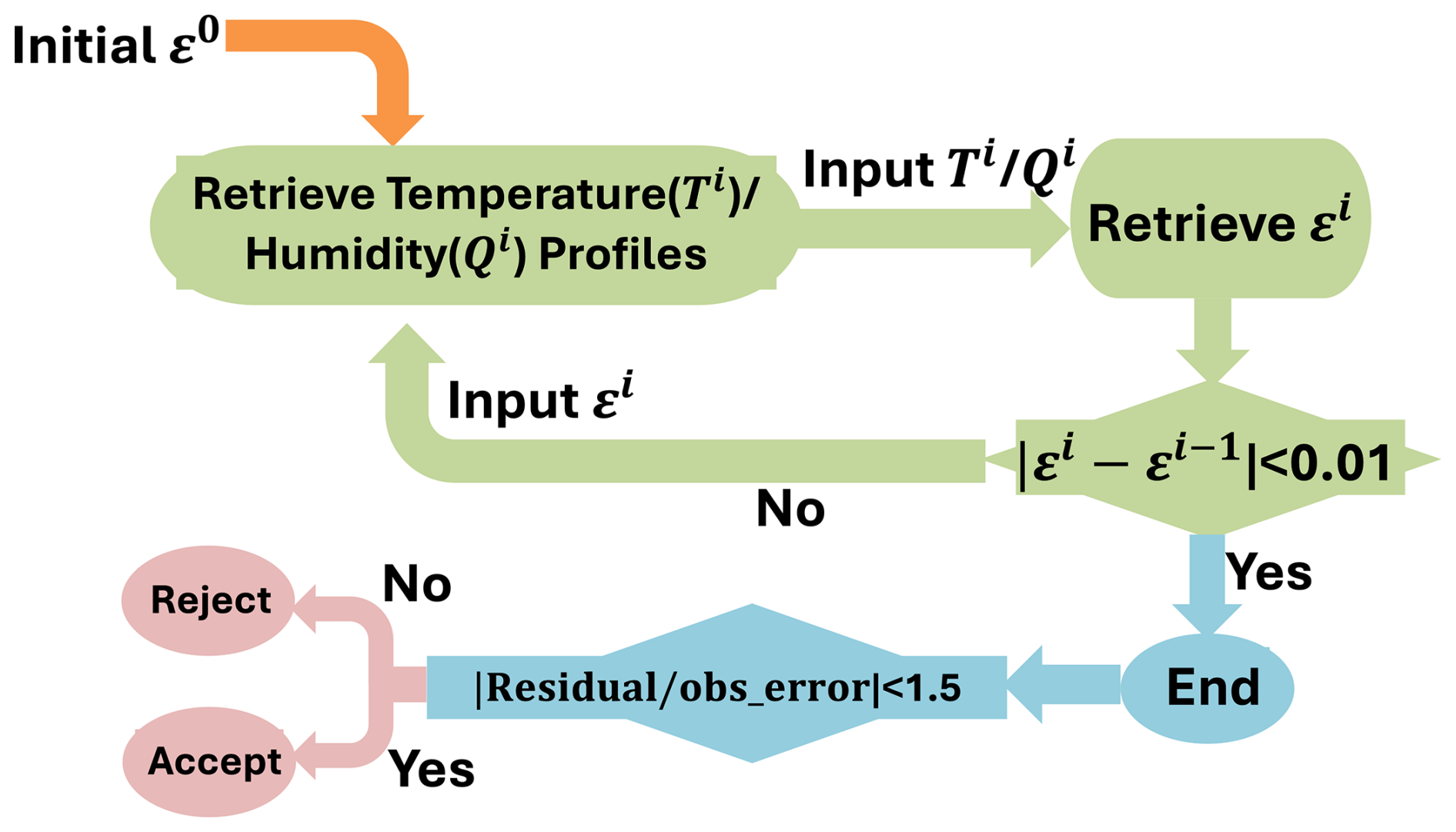
Figure 4 Flow diagram of the iterative retrieval process. The process starts with an initial guess of surface emissivity ε⁰ to retrieve temperature Tⁱ and humidity profiles Qⁱ, which are then utilized to adjust the surface emissivity εⁱ for subsequent iterations. Residuals are defined as the difference between observed and modeled brightness temperature and assessed against the observation noise equivalent delta temperature. Any residual falling within 1.5 times the noise equivalent delta temperature is considered a valid match. The final outcomes are the temperature and humidity profiles alongside the surface emissivity.

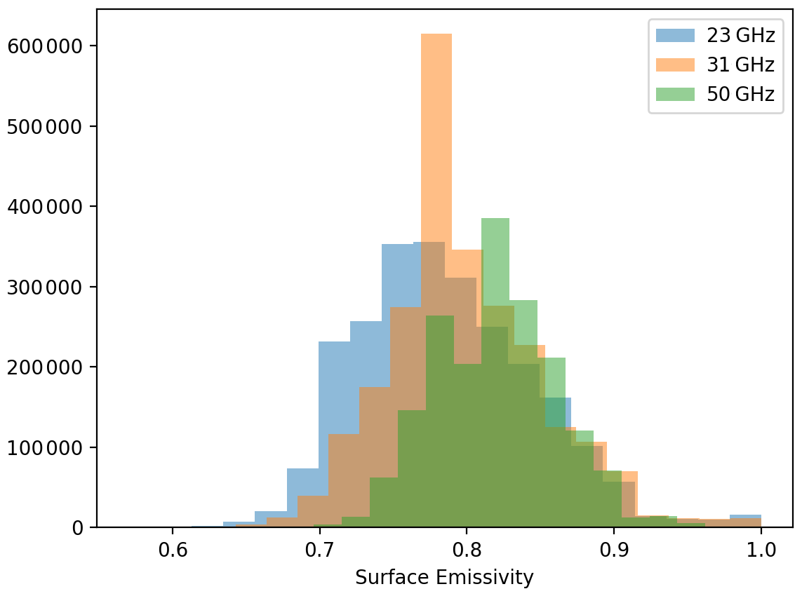
Figure 5 Histogram of AMSU-A surface emissivity values at 23, 31, and 50 GHz over the Antarctic region during 2016. These values are obtained from the AMSU-A emissivity data archive. The median emissivity across these frequencies is near 0.8, which serves as the initial value (ϵ₀) in our iterative retrieval process.

3.2 Forward Model – Radiative Transfer Model

RTTOV (Radiative Transfer for TOVS¹) is a fast radiative transfer code widely used in atmospheric remote sensing research (Saunders et al., 2018). The model incorporates detailed representations of atmospheric properties, including temperature, humidity, pressure, and optionally, trace gases, aerosols, and hydrometeors, together with surface parameters and viewing geometry, allowing for accurate simulations of radiative transfer processes in diverse atmospheric conditions. We incorporate a Python interface written for RTTOV v11.3. The model was not only used to calculate radiances but also to calculate the associated Jacobians. The profile is assumed to be linear between the vertical grid points. The grid used is close to equidistant in the logarithm of the pressure; hence, it is approximately equidistant in altitude. RTTOV computes the top-of-atmosphere radiances from both atmospheric and surface emission in each of the sensor channels. The radiance can be represented as

$$\begin{array}{}\text{(1)}& \begin{array}{rl}L\left(\mathit{\nu }\right)& ={\int }_{{\mathit{\tau }}_{\mathrm{s}}}^{\mathrm{1}}B\left(\mathit{\nu },T\right)\mathrm{d}\mathit{\tau }+\left[\mathrm{1}-{\mathit{\epsilon }}_{\mathrm{s}}\left(\mathit{\nu }\right)\right]\cdot {\mathit{\tau }}_{\mathrm{s}}^{\mathrm{2}}\left(\mathit{\nu }\right)\\ & \cdot {\int }_{{\mathit{\tau }}_{\mathrm{s}}}^{\mathrm{1}}{\displaystyle \frac{B\left(\mathit{\nu },T\right)}{{\mathit{\tau }}^{\mathrm{2}}}}\mathrm{d}\mathit{\tau }+{\mathit{\epsilon }}_{\mathrm{s}}\left(\mathit{\nu }\right)\cdot {\mathit{\tau }}_{\mathrm{s}}\left(\mathit{\nu }\right)\cdot B\left(\mathit{\nu },T_{\mathrm{s}}\right),\end{array}\end{array}$$

where L is the radiance at frequency ν; B(ν,T) is Planck's law; τ is the transmittance from the top of the atmosphere to depth τ, and τ_s is the transmittance from the top of the atmosphere to the surface, both of which depend mostly on oxygen and water vapor absorption; ε_s is the surface emissivity, while 1−ε_s is the respective surface reflectivity, and T_s is the surface skin temperature. The three terms on the right-hand side correspond to the upwelling atmospheric emission, the downwelling atmospheric emission reflected by the surface, and the surface emission, respectively.

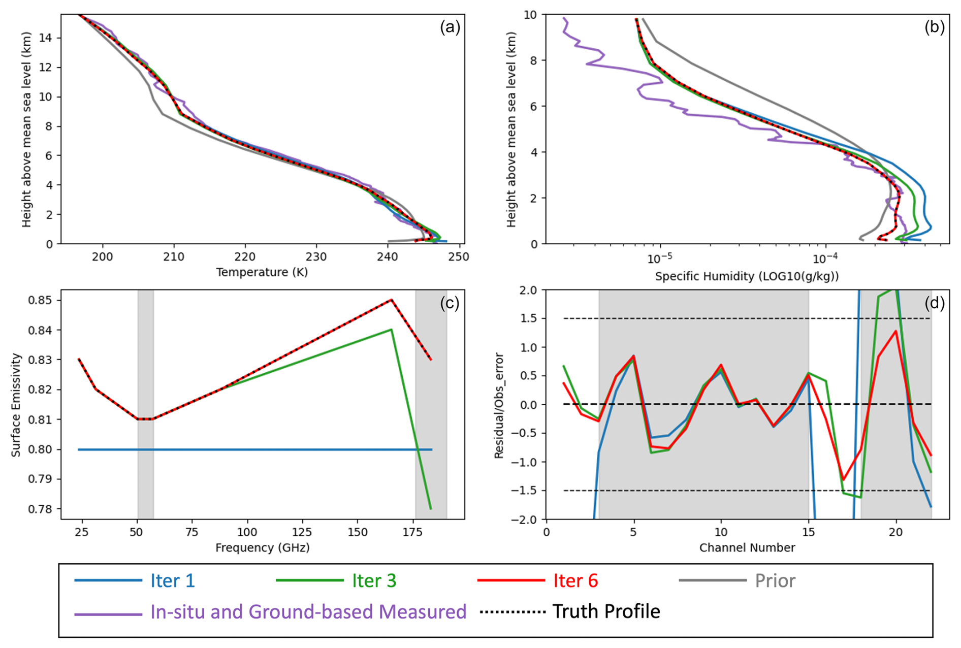
Figure 6 Retrieved temperature profiles (a), specific humidity profiles (b), and frequency-dependent surface emissivity (c) over six iterations (for clarity, only iterations 1, 3, and 6 are displayed). Panel (d) shows the residual divided by the observation noise (the model's fit is considered good when the absolute residuals at all frequencies are less than 1.5 times of the noise, indicated by the dashed lines). The iteration process converges within six iterations. The gray curve shows the prior for the temperature and humidity profiles. In the bottom two figures, the oxygen and water vapor absorption frequency bands/channels are shaded in gray. In panels (a) and (b), the purple curve shows the radiosonde in situ measurements. The black dotted line shows the reference profiles retrieved using the radiosonde reference emissivity. This demonstrated example is a particularly good fit where the retrieved surface emissivity closely matches ARM-derived values; not all cases show this level of agreement.

3.3 Retrieved profiles

We utilized our iterative retrieval method, as described in Sect. 3.1, on the ATMS data collected over the Antarctica region during 2016. Figure 6 presents an example of the retrieval evolution over six iterations, including temperature profiles (top left), specific humidity profiles (top right), and frequency-dependent surface emissivity (bottom left). The bottom right panel shows the residual (the difference between observation and model) divided by the observation noise. As discussed in Sect. 3.1, if the residuals for all frequencies/channels are under 1.5 times of the noise, the model is considered a valid match. Following six iterations, we observe convergence in the iterative process. Figure 6 shows temperature profiles up to 16 km above sea level and specific humidity profiles up to 10 km, corresponding to the altitude range covered by available radiosonde data. In the upper two panels, the purple curves display the radiosonde in situ measurements, used to validate the iterative retrieval algorithm. The radiosonde measurements reveal fine-scale temperature and humidity structures – with vertical resolution ranging from 20 m to a few hundred meters – that the microwave radiometer-based algorithms cannot resolve. Despite these fine features, the temperature profile obtained through iterations matches the radiosonde measurements. The specific humidity below 6 km also shows good agreement with the measurements. However, the retrieval method becomes less sensitive above 6 km, primarily due to humidity levels that are orders of magnitude lower at higher altitudes.

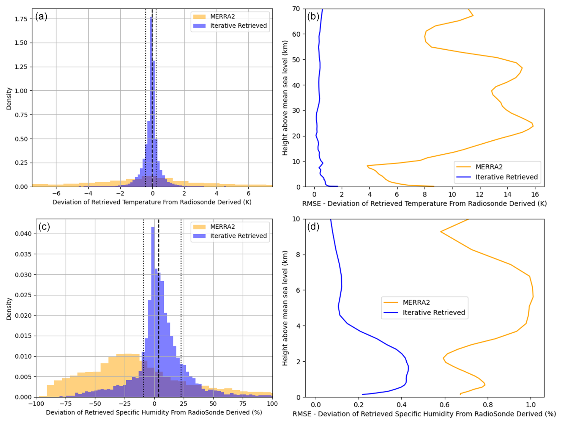
Figure 7 Histogram of the differences between atmospheric profiles retrieved by our iterative algorithm and the radiosonde reference profiles. Panels (a) and (b) show temperature differences below 70 km (K), and panels (d) and (d) show specific humidity differences below 10 km, expressed as a percentage relative to the reference profiles. We use percentage differences for specific humidity to account for its strong vertical gradient, which spans approximately 2 orders of magnitude; this approach avoids biasing the evaluation toward near-surface values. In the left column, dashed black lines represent the median and the 68 % confidence interval (one standard deviation) in each panel. Same histograms for the MERRA-2 profiles are included as a baseline, demonstrating that the iterative retrieval method improves agreement with observations by reducing deviations in both temperature and humidity. The right column show the root mean square error (RMSE) with respect to altitude.

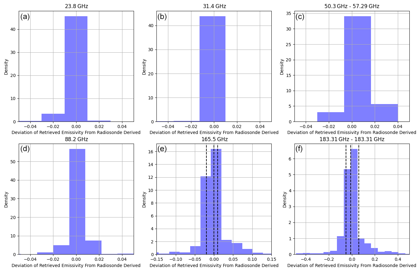
Figure 8 Histogram of the surface emissivity retrieved in our study compared to the radiosonde reference value. The dashed black lines represented the median value and the 68 % confidence intervals (one standard deviation) in (e) and (f).

As shown in Eq. (1), when atmospheric profiles are known, the observed brightness temperature from the top of the atmosphere can be expressed as a linear function of the surface emissivity. By combining radiosonde-measured atmospheric profiles with ATMS brightness temperatures, we compute the surface emissivity at ATMS frequencies, referred to as the radiosonde reference surface emissivity (the black dotted line, the lower left panel in Fig. 6). Our iteratively retrieved surface emissivity (red curve) is in good agreement with these radiosonde reference values. However, at 183 GHz – the water vapor absorption band – surface emission is tightly coupled with near-surface humidity, making accurate emissivity retrieval more difficult. As a result, the iterative method may yield less reliable results at this frequency (see Sect. 4.1). Using the reference surface emissivity, the black dotted lines in the upper panels of Fig. 6 represent the best-fit atmospheric profiles achievable with ATMS's 22 channels, serving as a benchmark for evaluating our iterative retrieval approach. The comparison between the radiosonde reference profile and the iterative retrieved profile in the upper panels indicated a high level of consistency.

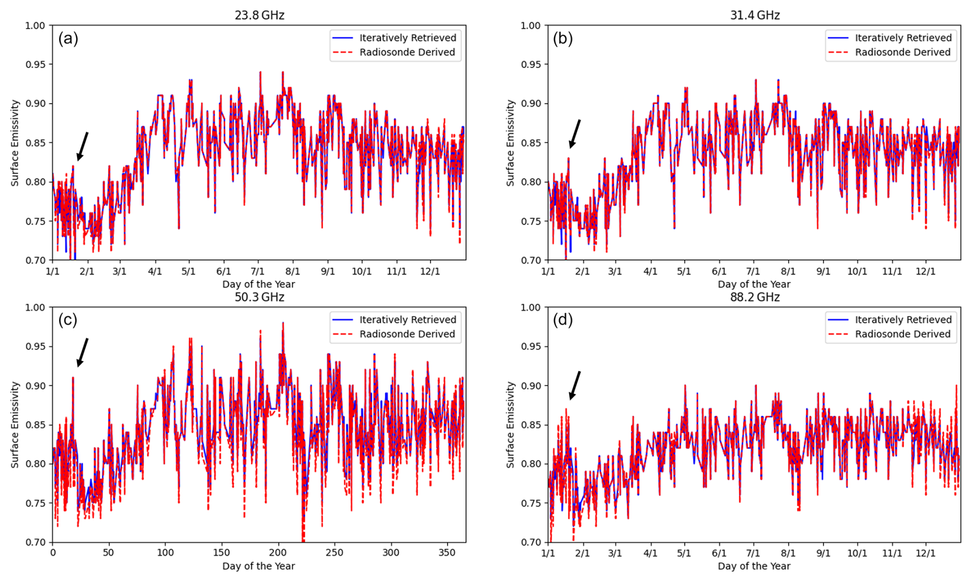
Figure 9 McMurdo Radiosonde Station (77.85° S, 166.66° E). Surface emissivity from November 2015 to the end of 2016 at three window frequencies (23.8, 31.4 and 88.2 GHz) and the oxygen absorption band (50–58 GHz). The blue curve represents values from our iterative algorithm and the red dashed line shows values derived from the radiosonde measurements. Two melting events occurred in mid-December and mid-January, pointed out by the black arrows. The x axis shows the month of the year, from 1 January 2015 to 31 December 2016.

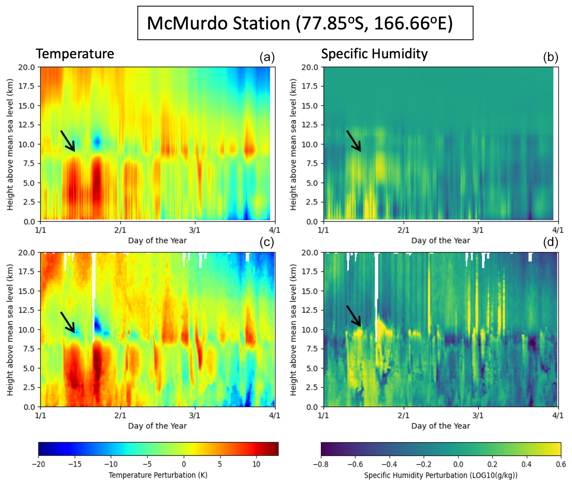
Figure 10 McMurdo Radiosonde Station (77.85° S, 166.66° E). Temperature and specific humidity perturbations during January to March 2016. The deviations from average values are displayed for that period. Panels (a) and (b) present results from our iterative algorithm, while the bottom row shows data from radiosonde measurements. Melting events in mid-January correspond to the temperature and humidity increases around the same time. The x axis shows the month of the year, from 1 January 2016 to 31 March 2016. The temporal resolution in the map is based on an interpolation of ATMS-observed data time intervals, which are approximately a few hours apart.

4 Validation and discussion

We assess the performance of our iterative retrieval method by comparing the retrieved atmospheric profiles with radiosonde measurements. This comparison demonstrates both the capability and limitations of our approach in capturing seasonal variations and surface–atmosphere interactions across Antarctica.

4.1 Mid-January 2016 melting event near the Ross Ice Shelf

In this section, we examine the atmospheric and surface conditions during the mid-January 2016 melting event by analyzing retrieval results at three key Antarctic sites – McMurdo Station, WAIS Divide, and Ross Ice Shelf – over the same time period, each of which shows corresponding variations in atmospheric profiles, surface emissivity, or both during the melt.

4.1.1 McMurdo Station

The McMurdo Radiosonde Station is located on Ross Island at coordinates 77.85° S, 166.66° E. In 2016, radiosonde observations were obtained with high temporal resolution at this station. Figure 7 presents a histogram of the differences between atmospheric profiles retrieved by our iterative algorithm and the radiosonde reference profiles as described in Sect. 3.3. The upper panels depict the temperature difference below 70 km height, while the lower panels show the specific humidity difference below 10 km height, spanning the entire year of 2016. The left panels show the median value and the 68 % confidence intervals (1 standard deviation). The accuracy of the temperature profile retrieval was high, with a standard deviation of 0.5 K. However, while most humidity variations were detectable (to be discussed further in the next paragraph), the absolute value was not precise compared to the measurement, with a standard deviation of approximately 25 %. The humidity was strongly linked to the surface emissivity at 183 GHz. In addition to the iteratively retrieved profiles, we also include histograms of deviations for the MERRA-2 archived profiles as a baseline. The results indicate that the iterative retrieval approach improves accuracy in both temperature and humidity, yielding distributions more closely aligned with radiosonde-derived observations. Fig. 8 shows the histogram displaying the difference between the surface emissivity retrieved iteratively and the radiosonde reference value. The surface emissivity retrieved iteratively is highly accurate within a range of ± 0.01 for window channels like 23.8, 31.4, and 88.2 GHz. In the oxygen absorption band between 50 and 58 GHz, most of the retrieved surface emissivity values fall within ±0.02 of the radiosonde reference value, aligned with the fact that retrieved temperatures have a one-sigma difference within ±0.5 K from the actual value. The channels above 165 GHz are affected by water vapor absorption. At 165 GHz, the emissivity retrieval shows a standard deviation of 0.03, while at 183 GHz, the standard deviation increases to ∼ 0.1. These discrepancies are too substantial to permit accurate retrieval of the humidity profile. An independent estimate of the ice sheet surface emissivity is required to separate the effects of ice sheet emissions and atmospheric humidity.

The changes in surface emissivity over the year provide information about melting events in the ice sheet. Figure 9 presents surface emissivity from November 2015 to the end of 2016 at three window frequencies and near the oxygen absorption band. The blue curve represents values obtained from our iterative algorithm, while the red dashed line shows the radiosonde reference values. These values are in good agreement with each other. Two melting events were observed around mid-December 2015 and mid-January 2016, as indicated by the black arrows. The melting event in mid-January was more significant. Following the melting event, the emissivity decreased due to ice crust formation within the surface snow during the refreezing, which increases scattering and depresses brightness temperature, resulting in reduced effective emissivity. Figure 10 displays temperature and specific humidity perturbations from January to March 2016, covering the period of the melting events and the availability of radiosonde measurements. These perturbations show deviations of the profiles from the average values during the specified period (from 1 January to 31 March 2016). The top row shows results from our iterative algorithm, while the bottom row shows profiles measured using radiosonde. Despite the higher vertical resolution in radiosonde measurements, our iterative algorithm captures the temperature and humidity variations effectively. The melting events in mid-January corresponded to increases in near-surface temperature and humidity, as indicated by the black arrows. Temperature increased by over 10 K during the melting event.

4.1.2 WAIS Divide Station

The WAIS Divide Station is located at coordinates 79.468° S, 112.086° W, with an altitude of approximately 1.8 km above sea level. Detailed radiosonde measurements were taken between 1 and 15 January 2016. Figure 11 compares the temporal fluctuations of temperature and specific humidity throughout January, along with surface emissivity (bottom panel), between the iterative retrievals (top row) and radiosonde measurements (middle row). By utilizing the iterative retrieval method, we were able to accurately track the rise in temperature and humidity from 10 to 15 January, aligning with the melting of the Ross Ice shelf as recorded at McMurdo Station in mid-January. In contrast to the surface emissivity changes observed at McMurdo Station, no substantial variations in surface emissivity were noted at the WAIS Divide Station, indicating stable ice crust structures and limited snowfall during the summer months. Although near surface temperatures increased, they did not reach levels sufficient to initiate melting at this inland location.

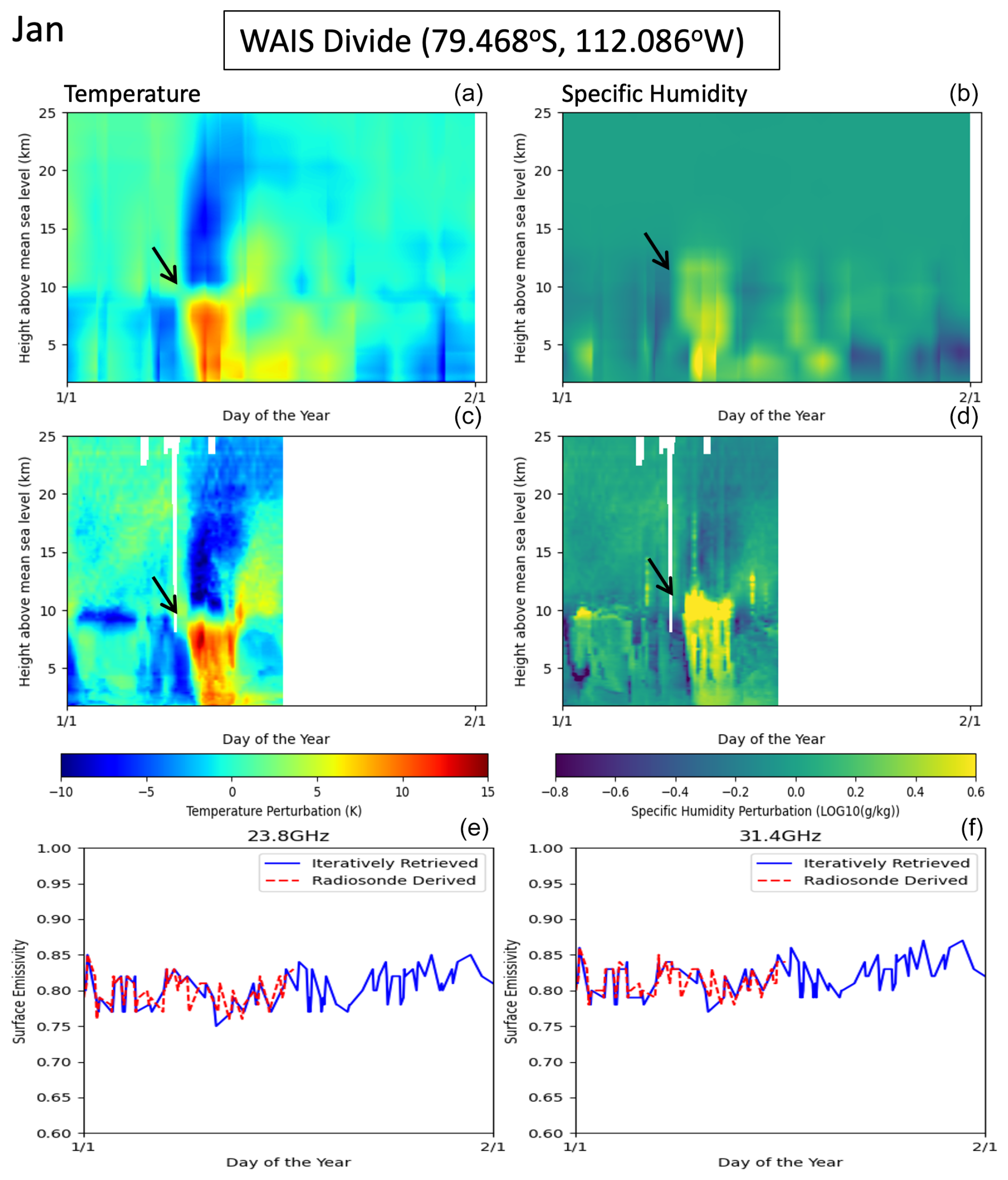
Figure 11 WAIS Divide Radiosonde Station (79.468° S, 112.086° W). Temperature and specific humidity perturbations during January 2016. The deviations from average values are displayed for that period. The top row presents results from our iterative algorithm, while the middle row shows data from radiosonde measurements. The x axis shows the month of the year, from 1 to 31 January to 2016. Bottom panels: surface emissivity at two window frequencies (23.8, 31.4 GHz). The blue curve represents values from our iterative algorithm and the red dashed line shows values derived from the radiosonde measurements.

4.1.3 Ross Ice Shelf

In January 2016, a significant surface melting event was documented that impacted a significant section of the Ross Ice Shelf (Nicolas et al., 2017; Mousavi et al., 2022; de Roda Husman et al., 2024; Hansen et al., 2024). The melting is associated with the strong and continuous transport of warm marine air to the region, likely influenced by the concurrent powerful El Niño event. The broad atmospheric fluctuations during and following the melting incident are found to be established by the El Niño event and mitigated by the positive Southern Annular Mode. These atmospheric changes are identified by our iterative method, as illustrated in Fig. 10 and Fig. 11. We present findings at the coordinates 83° S, 153° W at the center of the melting incident. As indicated in Fig. 12, there is a sharp rise in surface emissivity from 23.8 to 58 GHz, indicating surface melting over ice sheets and the presence of liquid water in the snowpack. Our iterative analysis of temperature and humidity perturbations captures the significant and vertically extensive intrusion of marine air from 10 to 13 January.

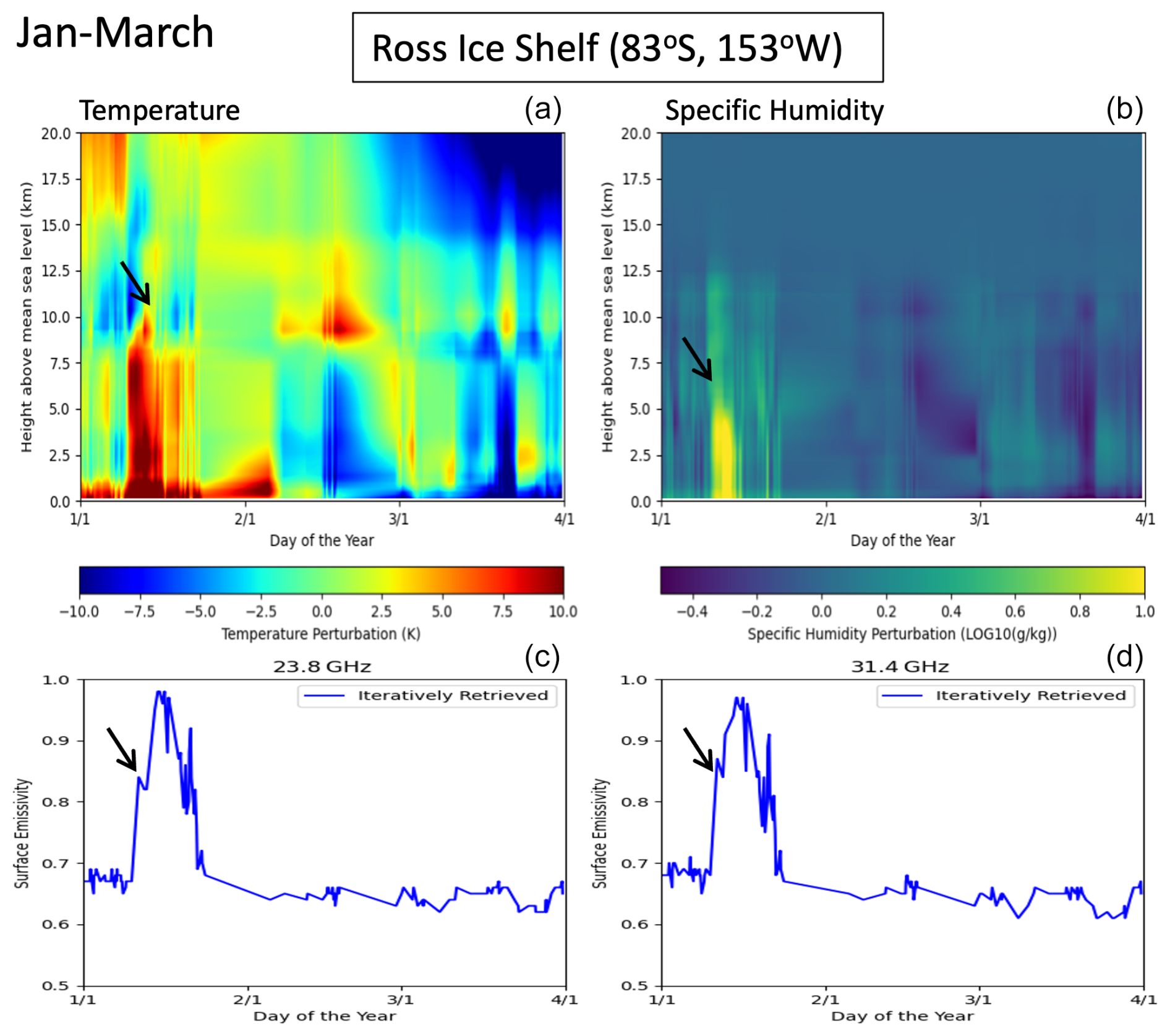
Figure 12 Ross Ice Shelf (83° S, 153° W). Temperature and specific humidity perturbations during January 2016 to March 2016. The deviations from average values are displayed for that period. The results are retrieved using our iterative algorithm. The x axis shows the month of the year, from 1 January 2016 to 31 March 2016. Panels (c) and (d): Surface emissivity at window frequencies (23.8, 31.4). The blue curve represents values from our iterative algorithm. The melting events occurred in mid-January, indicated by the black arrows.

4.2 West and East Coast ice shelves during 2016

In the Antarctica region, ice shelves cover approximately 1.5 million square kilometers and include major formations such as the Ross, Ronne-Filchner, and Larsen Ice Shelf. Ice shelf melt can lead to an accelerated ice discharge from the land into the ocean, significantly contributing to the global sea level rise. Melting events over these ice shelves are, therefore, critical to understanding and predicting future sea level changes.

The West Coast of Antarctica is home to several ice shelves, including the Larsen C, Wilkins, and George VI Ice Shelf, all situated on the Antarctic Peninsula. These ice shelves exhibit similar annual variations in surface properties. Notably, multiple surface emissivity increases are observed throughout the year (Fig. 13, upper left panel). labeled as events 1 through 8. Figure 14 presents the temperature and humidity perturbations associated with these surface emissivity changes, with each event number indicated. These emissivity changes are generally correlated with increases in atmosphere temperature and humidity, though they likely arise from a range of underlying causes. Figure 13's upper middle panel displays the skin temperature data from ERA5 (Hersbach et al., 2023), with the black dashed line representing the melting point at 273 K. During the summer months (January to March and November to December), increased emissivity corresponds to elevated skin temperatures reaching the melting threshold. An additional melting event detected in early May (event 4) is attributed to concurrent rises in both near-surface atmospheric temperature and skin temperature. Conversely, the increased emissivity observed in late May (event 5) is attributed to rainfall. These findings underscore the complex interplay of climatic factors driving the surface emissivity change on the Antarctic Peninsula's ice shelves, highlighting the sensitivity of these regions to both temperature and precipitation changes.

On the other hand, East Coast ice shelves, such as the Amery and Shackleton Ice Shelf, exhibit very difference yearly variations in surface conditions. Unlike the complex interactions observed around the West Coast, potential melting events on the East Coast – indicated by increases in surface emissivity as shown in Fig. 13 (lower left) – are detected exclusively during the summer months of January and December. According to ERA5 data (Fig. 13, lower middle and right), the East Coast experiences extremely dry conditions with nearly no precipitation of rain. These melting events are attributed solely to the increase in near-surface atmospheric temperature and skin temperature, which rise above the melting point during the summer.

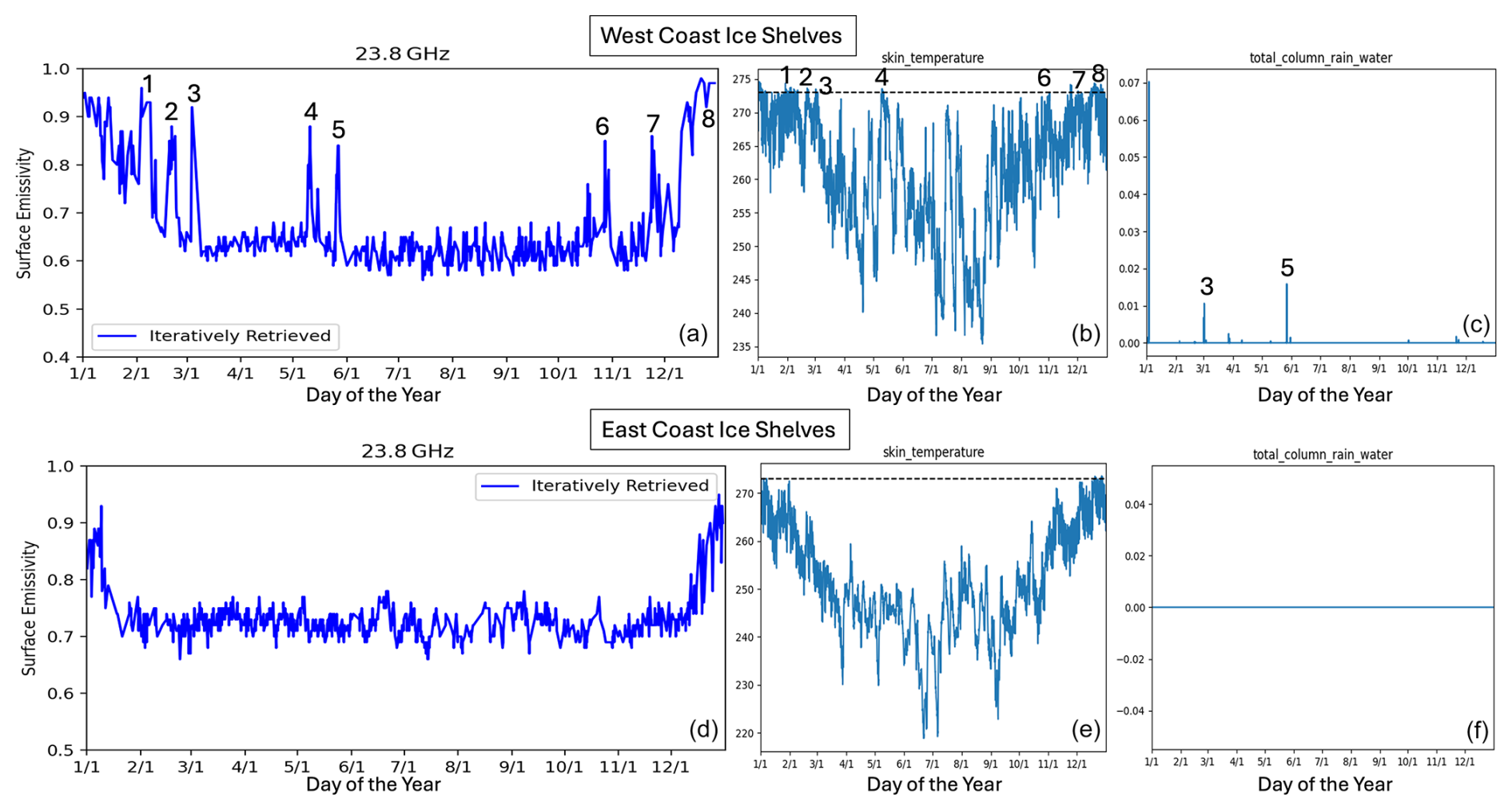
Figure 13 (a–c) West Coast – Larsen C Ice Shelf (67.5° S, 62.5° W). Surface emissivity variation at 23.8 GHz (a, d) shows a few significant increases during summer months and May. The results are retrieved using our iterative algorithm. A few emissivity increases are observed (labeled 1 through 8). Skin temperature (b, e) and precipitation of rain (c, f) from ERA5 are presented. The x axis shows the month of the year, from 1 January  to 31 December 2016. Lower row: East Coast – Amery Ice Shelf (70° S, 71° E). Surface emissivity variation at 23.8 GHz (a, d) shows potential melting events only during the summer months

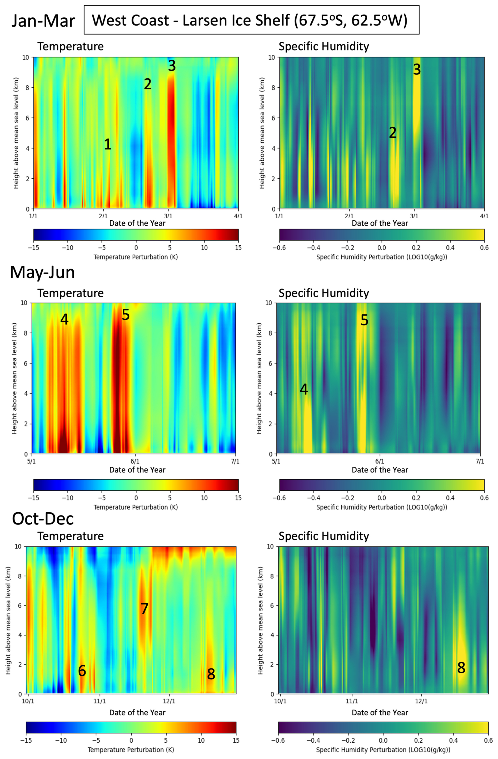
Figure 14 Larsen C Ice Shelf (67.5° S, 62.5° W). The corresponding temperature or humidity perturbations during the emissivity increase events – first labeled in Fig. 13 – are shown here and indicated using the same event numbers.

5 Conclusion

This study presents a novel iterative retrieval algorithm that couples atmospheric profile retrieval with surface emissivity estimation, applied to ATMS observations across Antarctica. This coupled approach enables improved retrieval of atmospheric states in the challenging conditions of polar environments where surface emission is complex and temporally variable due to melting and refreezing events. Validation against high-resolution radiosonde measurements from multiple Antarctic stations in 2016 demonstrates the algorithm's capability in retrieving atmospheric temperature profiles, with a typical retrieval accuracy of ±0.5 K. Surface emissivity estimates at transparent window and oxygen absorption channels (i.e., 23.8–88.2 GHz) are accurate within ±0.01–0.02. However, atmospheric humidity retrieval accuracy diminishes at higher frequencies, especially near the 183 GHz water vapor absorption band, where emissivity is entangled with near-surface humidity contributions. Water vapor retrievals, though able to resolve temporal variability, showed an absolute uncertainty up to 25 %, indicating that reliable retrieval of humidity requires independent emissivity estimates at water vapor-sensitive frequencies.

The study also reveals significant spatial variability across Antarctic regions. The Ross Ice Shelf exhibited pronounced emissivity and atmospheric changes during the 2016 mid-January melting event, aligning with observed marine air intrusions. In contrast, locations such as the WAIS Divide showed minimal emissivity variation despite similar atmospheric warming. West Antarctic coastal ice shelves (e.g., Larsen) exhibit complex emissivity variations throughout the year, influenced by both temperature fluctuations and precipitation events, whereas East Antarctic shelves (e.g., Amery) maintain more stable surface emissivity characteristics.

Future improvement hinges on integrating this retrieval framework with independent multi-frequency algorithms for estimating ice sheet surface properties (e.g., meltwater fraction, snow density), which can decouple surface and atmospheric signals. Such hybrid retrieval schemes are vital for robust long-term monitoring of polar climate feedbacks and for improving the accuracy of model-based predictions of how ice sheets will respond to future atmospheric conditions.