Short and Long-term Grounding Zone Dynamics of Amery Ice Shelf, East Antarctica

The detection of grounding line (GL) positions in Antarctica is crucial for investigating the stability and health of ice sheets and glaciers. In reality the GL position is not fixed and will migrate upstream or downstream in response to varying tidal states on an hourly to daily timescale, or in response to longer-term ice dynamic change. However, the magnitude of short and long-term GL migration is not well characterised in many parts of Antarctica. In this study, we employ the Differential Range Offset Tracking method to measure the tidal GL migration on the Amery Ice Shelf in East Antarctica. We delineate 32 GL positions for the year 2021, covering 1172 km of coastline. The results show that GL migration in this region is not solely dictated by tidal height or tidal difference but is also significantly influenced by ice velocity and subglacial bed topography, providing new insights into the GL dynamics of the region. We also observe significant long-term GL retreat in the eastern part of the Amery Ice Shelf relative to the MEaSUREs Antarctic GL Version2 derived from 2000 SAR imagery (Rignot et al., 2016), with the maximum retreat reaching up to 10 km. Our findings underscore the need for continuous, high-resolution GL monitoring around the whole Antarctic coastline, to improve predictive models of ice sheet responses to climate changes and their subsequent impact on global sea-level rise.

1 Introduction

Satellite-based observations acquired over the last 40-years have linked the recent mass loss of the Antarctic Ice Sheet to changes in the floating ice shelves (Paolo et al., 2015) that fringe the majority of its fast-flowing regions (Rignot et al., 2013) and critically control the rate of ice discharge into the ocean by buttressing upstream grounded ice (Gudmundsson, 2013; Haseloff and Sergienko, 2018). The grounding line (GL) is an Essential Climate Variable (Bojinski et al., 2014) where glacial ice shifts from being grounded on bedrock to floating on the ocean (Smith, 1991; Vaughan, 1994), and serves as a critical boundary condition in numerical ice sheet and glacier models that predict future glaciological evolution (Pattyn, 2018; Seroussi et al., 2014). The GL is a highly sensitive indicator of both glaciological and environmental change. Accurate measurements of the GL are essential for monitoring the stability of ice shelves and predicting potential collapse which is vital for accurately assessing the magnitude of future sea level rise (Joughin et al., 2014). Furthermore, tracking change in the GL location can shed light on the interplay between continental ice sheets and oceanic thermal dynamics, especially the impact of warm ocean water on ice shelf melt and retreat (Jenkins et al., 2018). Ice thinning and rising sea levels can cause GLs to retreat, whilst thickening or falling sea levels can cause them to advance (Friedl et al., 2020). Thus, continuous surveillance and analysis of GL positions hold significant importance as they support a broader understanding of global climatic patterns and their subsequent impacts on polar environments and global coastal communities (Stocker, 2014).

Recent advances in remote sensing technology have significantly enhanced our capability to monitor change in GL location, by employing methods such as Double Differential Synthetic Aperture Radar Interferometry (DDInSAR) (Goldstein et al., 1993; Rignot et al., 2016), SAR Differential Range Offset Tracking (DROT) (Joughin et al., 2016; Marsh et al., 2013; Wallis et al., 2024), Repeat Track Laser Altimetry (RTLA) (Fricker et al., 2009; Fricker and Padman, 2006), and Pesudo Crossover Radar Altimetry (Dawson and Bamber, 2017, 2020). Each technique offers unique advantages in terms of measurement accuracy, spatial and temporal coverage, and sensitivity to vertical and horizontal movement. In this study, we adopt the DROT method due to its ability to provide spatially continuous, high-frequency measurements under all weather conditions. Compared to RTLA, it is less affected by cloud cover and track spacing limitations, while unlike DDInSAR, it remains effective in fast-flowing or decorrelated regions where interferometric coherence is often lost. Typically, the GL is identified by locating the landward limit of ice flexure driven by tidal motion, however, this process is complicated by the influence of short-term sea level variations which may cause GL migration on an hourly to daily timescale. The short-term variation in GL migration is influenced by factors such as ocean tidal difference, local bed topography, atmospheric pressure, and the physical properties of the ice. Previous studies have used satellite observations to measure the size of this short-term, tidal GL migration which can vary significantly in different regions, ranging from several hundred meters to a few kilometres (Chen et al., 2023; Freer et al., 2023; Milillo et al., 2022). The grounding zone (GZ) in this paper is demarcated by a landward boundary at F_min and a seaward boundary F_max which encompasses the range of GL migration as influenced by tidal motion (Figure S1). Understanding the interplay between short-term tidal influences and long-term ice dynamic changes is critical for accurately measuring GL migration rates, and importantly, for ensuring that temporary variability is not mischaracterised as a more permanent change. Short-term GL migration provides valuable insight into the immediate response of ice shelves to tidal forces, while long-term migration reflects a broader response to climatic and environmental change. To improve the accuracy of long-term GL migration rate assessments it is essential to improve our understanding of how these short-term, spatially variable tidal movements affect the overall behaviour of ice sheet GLs.

The dynamics of GL migration on the Antarctic Ice Sheet are governed by a complex interplay of geophysical and oceanographic factors. From a long-term perspective, the thermal regime of adjacent ocean waters exerts a primary role, with elevated subglacial temperatures promoting basal melt and consequent GL retreat (Jenkins et al., 2018). Subglacial topography, especially the presence of retrograde slopes, is a pivotal control on the stability and progression of GL migration (Favier et al., 2014). The process of ice shelf buttressing, where floating ice shelves exert a stabilizing backpressure, is crucial; and reductions in buttressing strength due to ice shelf attrition or collapse may drive accelerated GL retreat (Rignot et al., 2011). Currently, ocean tide variations are considered the primary factor affecting the short-term GL migration. Rising tides increase buoyancy, lifting the ice shelf from the bed and causing the GL to migrate inland (Gudmundsson, 2006; Padman et al., 2018). The GL then returns to its most seaward position at low tide, with a slight time lag attributed to the ice's viscoelastic properties (Reeh et al., 2003). Variations in subglacial water pressure can also temporarily lift the ice, reducing friction and allowing the GL to move, such as from seasonal surface meltwater input to the ice-bed interface through supra-glacial lake drainage (McMillan et al., 2007), active subglacial lake drainage (Sundal et al., 2011) or change geothermal heat driven ice melt (Stearns et al., 2008). Beyond the subglacial system other factors influencing short-term, temporary GL variability include change in ocean currents (Jenkins et al., 2010) and atmospheric pressure (Walker et al., 2013). These factors can act independently or in combination, causing the GL to migrate temporarily. There is a lack of suitable data in the historical satellite archive with sufficient spatial and temporal resolution to characterise short-term GL variability, therefore, our understanding of the mechanisms controlling short-term GL migration is limited. New methods and the larger volume of data acquired by operational satellites such as the European Commission and European Space Agency (EC-ESA) Copernicus Sentinel missions are required to understand the internal mechanisms of the short-term GL migration and to better monitor the stability of ice shelves.

In this study, we use the DROT method to measure the temporal and spatial variation in the location of the GL on the Amery Ice Shelf (AmIS). Our research repeatedly maps the migration pattern of the GL across different tidal states in 2021, providing a detailed record of the GZ dynamics on this ice shelf. We assess the correlation between GL migration and geophysical factors such as ice velocity and subglacial bed topography, exploring the interdependent link between these variables. The results provide a refined perspective on the role of tidal action in shaping the transient behaviours of the GZ on AmIS, and we discuss the potential of DROT for accurately measuring the location and area of ice shelf pinning points. By combining the high temporal-resolution GL measurements obtained using the DROT method with established remote sensing techniques, we aim to improve our understanding of Antarctic GZ dynamics which will help improve the accuracy of sea-level rise projections in a warming climate.

2 Methods and Data

2.1 Study Area

The AmIS is a prominent feature in East Antarctica and is significant for its role in the continent's glacial dynamics. With an area of about 60 000 km², AmIS is the third largest ice shelf in Antarctica and the largest ice shelf in East Antarctica. AmIS is the terminus for three major glaciers, namely Fisher, Mellor, and Lambert, which form part of the expansive Lambert-Amery system that is responsible for draining approximately 16 % of the East Antarctic Ice Sheet (Galton-Fenzi et al., 2012). The AmIS is distinct from other Antarctic ice shelves due to its long, narrow sub-ice-shelf cavity and its location at the northernmost latitude (69° S) of the East Antarctic coastline, which exposes it to different environmental conditions. Unlike ice shelves in the Amundsen Sea and on the Antarctic Peninsula, AmIS has relatively low rates of basal melt, with modest thickening across the majority of its area and thinning at its most inland reaches (Davison et al., 2023), rendering it potentially less susceptible to rapid disintegration.

The AmIS's complex shoreline and GL have been the subject of extensive research for over half a century. Pioneering field surveys in the late 1960s laid the groundwork for our current understanding of the GL (Budd et al., 1982). Subsequent advances in satellite remote sensing technology enabled a more detailed redefinition of the GL position, employing numerical terrain models that incorporated SAR imagery from the ERS-1 and -2 missions complemented by data measuring ice thickness and density (Fricker et al., 2002). The evolution of satellite data use has markedly improved the precision with which we map the GLs on the AmIS. Techniques have evolved to include a combination of Synthetic Aperture Radar Interferometry (InSAR), Moderate Resolution Imaging Spectroradiometer optical imagery, and Ice, Cloud, and land Elevation Satellite (ICESat) laser altimetry data (Fricker et al., 2009). By employing data from multiple satellite missions, such as Landsat-8 and ICESat, studies have investigated the stability of the AmIS's GL's dynamics, showing that its location is relatively stable over the observed time periods (Xie et al., 2016). Earlier studies of the AmIS iceberg calving cycle predicted that the ice shelf may not experience a major iceberg calving until around 2025 or later (Fricker et al., 2002), and on 25 September 2019 a calving event was observed producing the D-28 iceberg, which was the largest iceberg calving event on this ice shelf since 1960 (Francis et al., 2021). Collectively these results highlight the need for continuous satellite observations of Antarctic ice shelves and studies that monitor major change.

2.2 Differential Range Offset Tracking

DROT is a dynamic method for GL detection that measures tidally induced vertical displacement of the ice shelf surface, by applying the differential principle of DDInSAR (Rignot, 1998) to fields of horizontal ice velocity obtained from SAR intensity offset tracking (Hogg, 2015; Joughin et al., 2016; Marsh et al., 2013; Wallis et al., 2024). To produce the DROT measurements we used the following four steps:

• i.

  SAR Image Acquisition. The Sentinel-1 satellite constellation, a cornerstone of the EC-ESA Copernicus Programme, represents a leap forward in Earth observation capabilities (Snoeij et al., 2009). Comprised of two satellites, Sentinel-1A and Sentinel-1B (which ceased operating on 23 December 2021), this system is equipped with an advanced C-band SAR instrument. The high-resolution, global coverage SAR images are acquired irrespective of weather or daylight conditions and are used for a myriad of applications including maritime surveillance, land surface monitoring, and disaster management. Sentinel-1 satellites facilitate consistent monitoring of specific areas, including the polar region, with a repeat cycle of 12 d when operating independently or 6 d when the two satellites acquire data in tandem. In this study, we utilize the Sentinel-1 images acquired in the interferometric wide swath (IW) mode to measure the GZ. In IW mode, Sentinel-1 satellites employ a technique called Terrain Observation by Progressive Scans to steer the satellite's radar antenna to obtain multiple swaths of data, which are then combined to form a single wide image. With a swath width of approximately 250 km, the IW mode offers a balance between swath coverage and spatial resolution, which is approximately 5 m by 20 m in range and azimuth directions respectively, for dual-polarization data. The dataset utilized in this study was collected over one-year period, beginning in January 2021 and concluding in December 2021.

• ii.

  Intensity Offset Tracking: We employed the SAR intensity offset tracking method (Strozzi et al., 2002) to measure the slant-range and azimuth registration offsets between a pair of SAR images. This method generates offset fields by employing normalized cross-correlation on patches from the real-valued SAR intensity images (Paul et al., 2015; Strozzi et al., 2002). The accuracy of detecting local image offsets is contingent upon the existence of nearly identical features within the SAR images, such as crevasses and unique radar speckle patterns. When the images maintain coherence, the speckle pattern within them can be correlated, allowing for highly accurate intensity tracking even with smaller image patches. Co-registration was achieved using precise orbit data available 20 d post-image capture, yielding an azimuth co-registration accuracy of 0.001 pixels. This precise alignment allows for the orbital offset to be effectively discounted, isolating the movement attributable solely to glacier dynamics. The geometry of a side-looking, off-nadir SAR sensor is such that a horizontal component is measured if any vertical displacement occurs in the slant-range direction. The size of this displacement depends on the angle from the local vertical at which the sensors signal intersects the Earth's surface, and the amplitude of any real vertical displacement. Consequently, the slant-range displacement fields we obtain over areas of floating ice simultaneously capture a real horizontal displacement caused for example by the flow of ice, and real vertical displacement originating from tidal motion of the floating ice. For each single intensity range offset tracking result, when translated to ground range, the tidal bias S can be estimated as the tidal change divided by the tangent of the incidence angle $S=\frac{{\mathit{\zeta }}_{\mathrm{2}}-{\mathit{\zeta }}_{\mathrm{1}}}{\tan \mathit{\theta }}$. S is the tidal bias, ζ₂ and ζ₁ are the true tidal height at the moments of SAR image acquisitions, θ is the incidence angle of SAR sensor, which is defined as the angle between the radar beam and the local vertical at the point where the radar beam intersects the Earth's surface. For example, at an incidence angle of 30°, a 1 m tidal change between two SAR image acquisitions generates a 1.73 m bias in the horizontal displacement. In this study, we used the CATS2008 Antarctic tide model (Padman et al., 2008) to generate ocean tidal height estimates. This ocean tide model estimates tidal movements within ice shelf cavities, achieving a noteworthy precision of 5 cm (Glaude et al., 2020). We applied inverse barometer effect (IBE) corrections using a 1 cm hPa⁻¹ conversion (Padman et al., 2003) from the fifth generation of ECMWF atmospheric reanalyses of the global climate (ERA-5) pressure anomalies, following the method described in Chen et al. (2023).

• iii.

  Displacement Differencing: A single Range Offset Tracking (ROT) displacement field over floating ice encompasses both the actual horizontal displacement from ice flow and a signal caused by vertical tide motion. As displacement from ice flow is much larger than tidal displacement, it would not be possible to measure the GL position from this data alone. In methodology analogous to DDInSAR, we therefore difference two ROT displacement fields derived from satellite passes with approximately identical imaging geometry, to produce a DROT measurement where constant ice flow displacement is removed, and the ocean tide motion signal is isolated. If the two images of each pair share the same time interval, differencing the datasets will remove the consistent horizontal displacement (assuming a steady ice velocity), whereas the ocean tidal height which is not constant through time will be visible as an anomaly (Joughin et al., 2016; Marsh et al., 2013). Depending on whether the two ROT displacement fields are constructed from three or four input SAR images, the differential tidal bias, ΔS, within a DROT displacement field relies on the sea levels, ζ_n, captured at the time of each SAR acquisitions:

  $$\begin{array}{}\text{(1)}& {\displaystyle }\begin{array}{rl}\mathrm{\Delta }S& ={\displaystyle \frac{({\mathit{\zeta }}_{\mathrm{3}}-{\mathit{\zeta }}_{\mathrm{2}})-({\mathit{\zeta }}_{\mathrm{2}}-{\mathit{\zeta }}_{\mathrm{1}})}{\tan \mathit{\theta }}}={\displaystyle \frac{{\mathit{\zeta }}_{\mathrm{3}}-\mathrm{2}{\mathit{\zeta }}_{\mathrm{2}}+{\mathit{\zeta }}_{\mathrm{1}}}{\tan \mathit{\theta }}}\\ & \text{(case of 3 input images)}\end{array}\text{(2)}& {\displaystyle }\begin{array}{rl}\mathrm{\Delta }S& ={\displaystyle \frac{({\mathit{\zeta }}_{\mathrm{4}}-{\mathit{\zeta }}_{\mathrm{3}})-({\mathit{\zeta }}_{\mathrm{2}}-{\mathit{\zeta }}_{\mathrm{1}})}{\tan \mathit{\theta }}}={\displaystyle \frac{{\mathit{\zeta }}_{\mathrm{4}}-{\mathit{\zeta }}_{\mathrm{3}}-{\mathit{\zeta }}_{\mathrm{2}}+{\mathit{\zeta }}_{\mathrm{1}}}{\tan \mathit{\theta }}}\\ & \text{(case of 4 input images)}\end{array}\end{array}$$
• iv.

  GL Measurement. To measure the GL location, the displacement fields from DROT must be distinctly divided into regions influenced by tidal bias and those that are not. In this study we do this by manually delineating the inland limit of tidal flexure in each DROT image, with the landward location where the displacement gradient begins to exceed zero determined to be the GL position. In the seaward direction, the location where the displacement gradient approaches zero again is interpreted as point H (as defined in Fig. S1 in the Supplement). Using both these positions we can obtain the width of the GZ from each DROT displacement field. Previous studies have used a threshold set close to zero to more automatically locate the position of GL (Wallis et al., 2024). However, in some cases this can be more complex as the ice shelf surface may exhibit considerable variations due to processes such as snow deposition, redistribution or surface melt, and surface deformation caused by ice flow. To ensure the GL is precisely located over a range of time periods we analysed the deformation gradient obtained from each DROT measurement.

3 Results

3.1 Grounding Zone Distribution

To detect the GLs, we construct DROT displacement fields using data acquired by the Sentinel-1a and -1b in 2021 following the approach introduced in Sect. 2.2. The capability to produce multiple GL observations under varying tidal conditions within a single calendar year facilitates the delineation of the GZ and improves the accuracy of longer-term GL migration measurements. We conducted the analysis using SAR images with a temporal baseline of 6 d, corresponding to frame 003 (orbits: 0834, 0839, 0843, 0848), with detailed information of selected SAR images presented in Supplement Table S1. We successfully produced a comprehensive GL dataset spanning 1172 km along the majority of the AmIS coastline (Fig. 1a and b). We extracted DROT deformation measurements along 18 profiles located across the GZ (Fig. 2a to r), which clearly shows the vertical displacement of the floating ice shelf alongside the absence of any displacement on the inland section of each profile for each period. This enables us to measure the inland limit of flexure experienced by the ice shelf and therefore delineate the GL location. We quantify the GZ width (as defined in Fig. S1) by measuring the distance between the most seaward and landward GL positions, tracing the trajectory of their migration. The width of the GZ derived from DROT, and its spatial variability around the AmIS coastline is also shown (Fig. 1c), which unveils a zone of ephemeral grounding extending over 1932 km² area. The limit of tidal flexure has migrated inland in 2021 by a range spanning several hundred meters to 14.2 km (Fig. 1c). Previous studies suggested that the GZ typically extends only a few hundred meters (Brunt et al., 2011; Christianson et al., 2016). However, with advances through data acquired by the ICESat-2 laser altimetry satellite, recent research has shown that this range can reach several kilometres. For example, tidal-induced GL migration of up to 15 km was observed at the Bungenstockrücken ice plain, far exceeding earlier estimates (Freer et al., 2023). This highlights the short-term variability of GZ dynamics, particularly in areas with significant tidal influences like AmIS. The GZ of AmIS varies in width depending on the coastal geometry. It is narrower (< 4 km) in areas with a smooth, straight coastline, such as profiles 1 and 2 (Figs. 1b and 2a and b), and wider in regions with indentations or constricted geometry, as seen in profiles 14 and 15 (Figs. 1b and 2n and o). This suggests that the GZ expands in more confined areas. Nevertheless, the total short-term GL migration distance could potentially be still larger than we have captured in this study in regions where the full tide range has not yet been sampled by the SAR acquisitions used in this study.

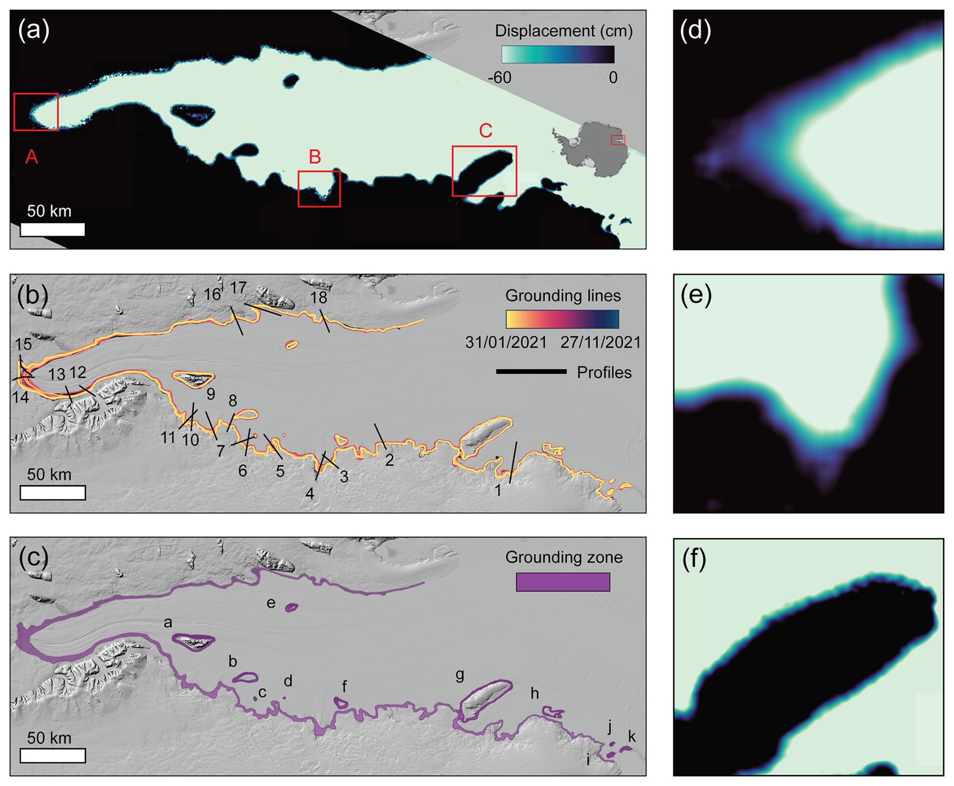
Figure 1 (a) An example of a DROT result produced from Sentinel-1 data acquired on 8 March 2021, 14 and 20 March 2021, with the colour scale corresponding to the amount of tidally induced vertical displacement. The location of zoom maps is also indicated (red box); (b) Chronological GL positions (coloured lines) mapped from 32 DROT results measured between January and November 2021. The colour gradient defines the acquisition date of each DROT measurement, with satellite data acquisition dates listed in Table S1. The location of cross-grounding zone profiles, labelled 1 to 18, is also shown (solid black line); (c) Summary map of GZ distribution (purple shading) for the AmIS, throughout the 11-month study period. Labels “a” to “k” indicate the locations of the 11 DROT-derived pinning points measured on the AmIS. The Reference Elevation Model of Antarctica (REMA) (Howat et al., 2019) is used as a basemap in subplots (a) to (c). (d–f) Zoomed in maps of the DROT displacement map for three locations labelled A to C in (a).

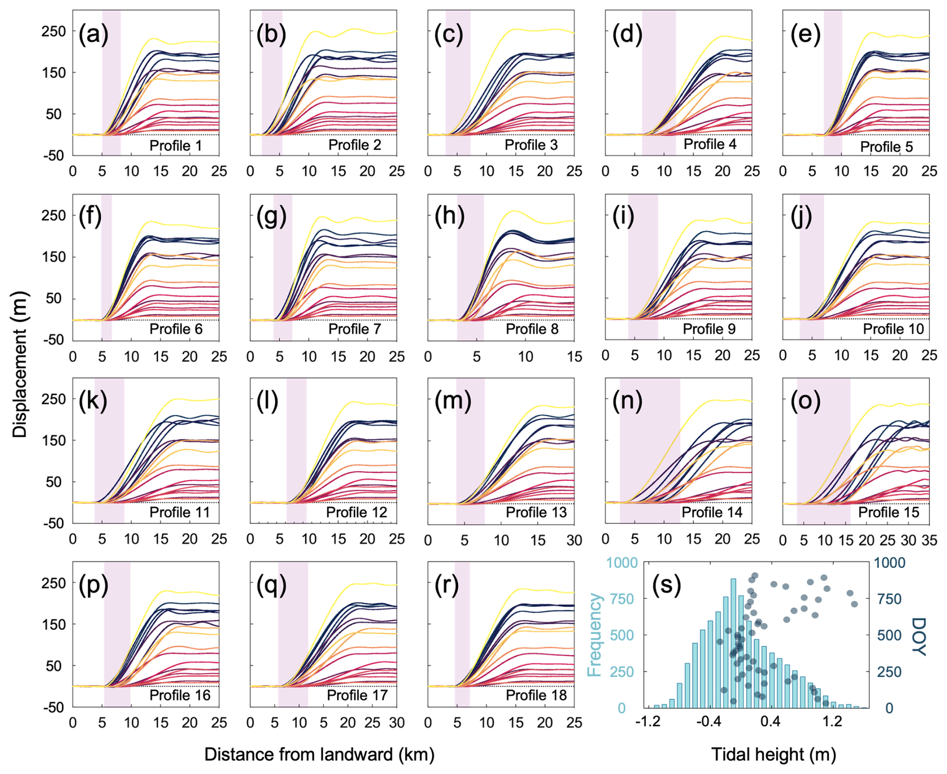
Figure 2 (a–r) DROT-derived displacements extracted along 18 profiles located perpendicular to the grounding zone, as shown in Fig. 1b. The colour of each line corresponds to the DROT measurement date (yellow is January 2021, purple is November 2021) (colours consistent with scale used in Fig. 1b), and light purple shading indicates the width of the measured GZ. (s) Distribution of tidal height recorded through the year-long study period (light blue bars), shown alongside tidal height at times of each SAR image acquisition (grey dots).

3.2 Comparison with Other Grounding Line Measurements

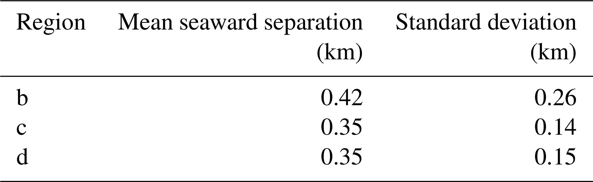
To assess the performance of the DROT method for GL detection we performed a comparative analysis with contemporaneous GL measurements made using the DDInSAR technique. We manually delineated the GL location in double differential interferograms produced from Sentinel-1 data acquired on the same dates as the DROT measurements used in this study (Fig. 3a). Weather processes at the ice sheet and shelf surface such as surface melt, snowfall and blowing snow affect the coherence of the DDInSAR images, therefore, it is not always possible to make GL measurements around the entire coastline of the AmIS using this technique. Nevertheless, these results enable us to directly compare the tidal deformation and GL location observed in the same region and time-period, using independent but complementary methods. Along the western and eastern coastlines of AmIS we observe a clear distribution of dense interferometric fringes in the double differential interferogram which corresponds to the GZ, and in line with previous studies we delineate the inland limit of these fringes to be the GL location. However, in the upstream part of AmIS where the Fisher, Mellor, and Lambert Glaciers converge, the rapid flow of ice causes a large displacement of the ice surface resulting in phase decorrelation, which makes it difficult to distinguish the GL boundary between in the DDInSAR fringe patterns. Where GL measurements were available from both techniques, we directly evaluated the performance of the DROT results quantitatively through a comparison to GL positions derived from both independent measurements (marked as b to d in Fig. 3a). Our analysis suggests that on average the DROT-derived GL positions are generally more seaward compared to those from DDInSAR, so this should be considered when assessing change from GL measurements produced from independent techniques (Fig. 3b.ii to d.ii). The DROT-derived GL's alignment with the DDInSAR measurements is shown to be precise within 0.5 km, with differences ranging from 0.35±0.14 to 0.42±0.26 km (Table 1), and coupled with the low standard deviation this underscores the reliability of the DROT method for accurately monitoring the DDInSAR GL location. This demonstrates the complimentary nature of both tidally sensitive GL measurement techniques and shows that the DROT method can be used alongside DDInSAR or at times when interferometric coherence does not exist.

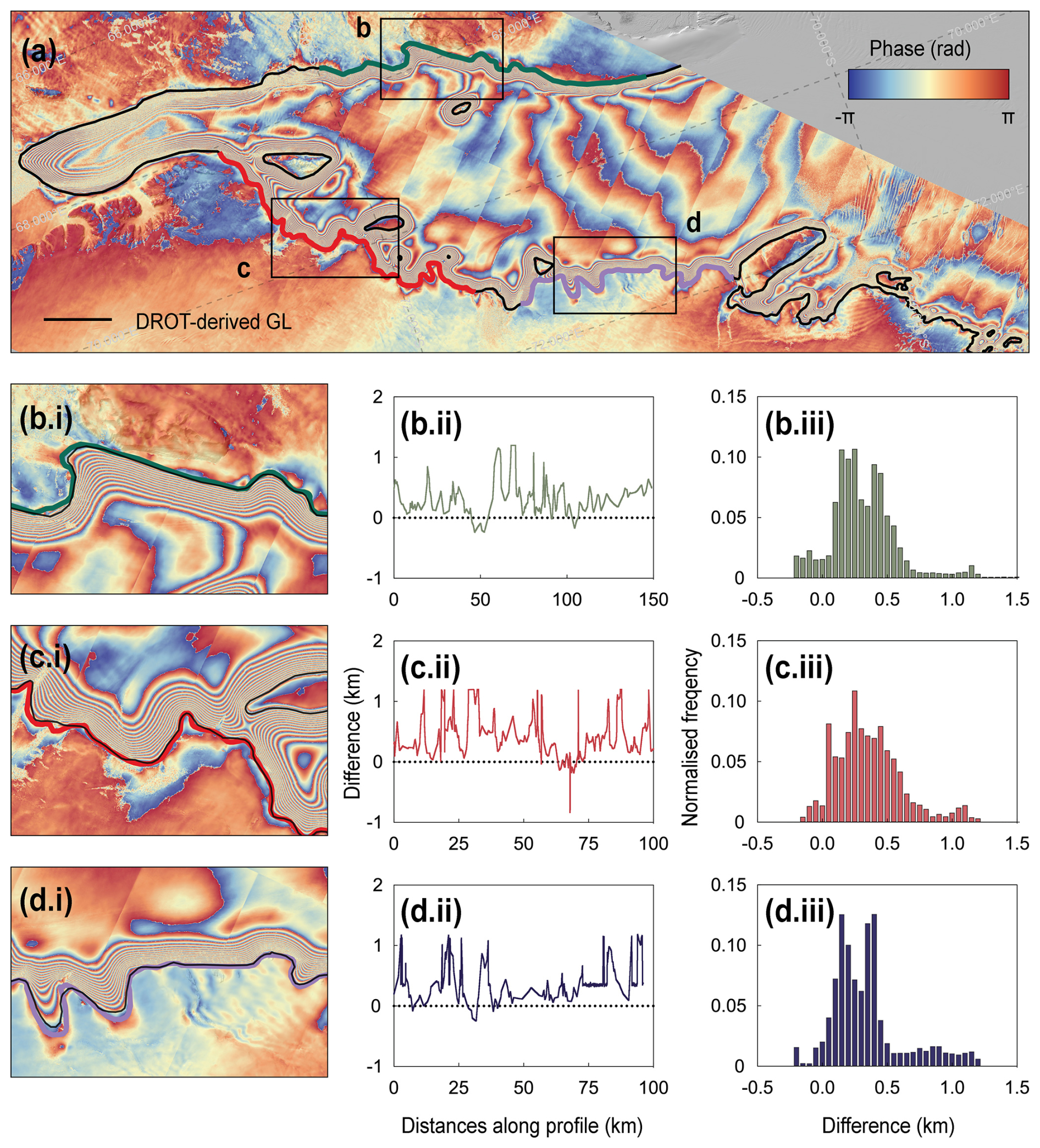
Figure 3 Comparison of DROT-derived GL and contemporaneous DDInSAR-derived GL for three locations on AmIS with high coherence: (a) A Sentinel-1 double differential interferogram from 31 May–6 June–12 June 2021, with the contemporaneous DROT-derived GL (black line), and reference lines (green, red and purple lines) also shown. These reference lines are extracted from the DDInSAR-derived GL results and correspond to the profiles analysed in (b.ii–d.ii) and the distribution histograms in (b.iii–d.iii). (b.i–d.i) Zoomed in map of three locations labelled b to d in (a). (b.ii–d.ii) Difference between DROT-derived GL and DDInSAR-derived GL the along the reference profiles (shown in Fig. 3a), where positive values indicate that the DROT-derived GL positions are located seaward of the DDInSAR-derived GL measurement. (b.iii–d.iii) Histograms show the distribution of differences between the two GL measurements along the reference profiles (shown in Fig. 3a).

Table 1 Mean seaward offset and standard deviation between the DROT-derived GL and contemporaneous DDInSAR-derived GL measured from 31 May–6 June–12 June 2021. Positive values indicate that the DROT-derived GL is located closer to the ocean compared to the DDInSAR-derived GL.

The MEaSUREs Antarctic GZ Version 1 (MAGZv1) dataset provides a comprehensive map of short-term GL migration zones across the Antarctic Ice Sheet using the DDInSAR technique (Rignot et al., 2023). We compared DROT-derived GZ results with the subset of MAGZv1 dataset over the AmIS, which is based on Sentinel-1 data acquired in 2018, to assess their spatial consistency. We first computed the Intersection over Union (IoU), defined as the area of intersection divided by the area of union (Fig. S2a), to evaluate the overall spatial agreement between the two GZ products. The comparison yielded an IoU of 0.44, indicating a moderate level of spatial overlap. In addition, we calculated recall and precision to quantify detection performance. Here, recall is defined as the fraction of the MAGZv1 GZ area that is correctly identified by the DROT-derived GZ, while precision refers to the fraction of the DROT-derived GZ area that overlaps with MAGZv1. The recall reached 0.84, suggesting that the DROT-derived GZ successfully captures the majority of the area defined by MAGZv1. However, the precision was relatively lower at 0.48, implying that over half of the area identified by DROT as GZ lies outside the extent of MAGZv1. This asymmetry reflects a broader delineation of the GZ by the DROT method, potentially capturing additional zones not included in the earlier dataset. We further evaluated the spatial offsets along the landward and seaward GZ boundaries (Fig. S2b–c). For the landward boundary, the DROT-derived GZ was positioned on average 460±700 m landward relative to the MAGZv1 boundary. For the seaward boundary, the offset was $-\mathrm{260}\pm \mathrm{660}$ m, indicating that the DROT extend farther seaward into the floating ice shelf (Fig. S2c.i and c.ii). These patterns suggest that our DROT-derived GZ results tends to resolve a broader GZ, with landward boundary positioned farther inland and the seaward boundary extending farther into the floating ice shelf compared to MAGZv1.

We attribute the differences observed between the DROT-derived GZ and the MAGZv1 product to a combination of methodological, temporal, and tidal factors. First, the two techniques are based on fundamentally different approaches. While MAGZv1 employs the DDInSAR method to detect vertical tidal flexure through interferometric phase change, the DROT technique measures displacement from SAR amplitude imagery, enabling GZ detection even in areas with low coherence. However, DROT has a slightly lower measurement sensitivity, typically on the order of 0.2–0.7 m, corresponding to a fraction of the ∼ 2.3 m range pixel in Sentinel-1 images, compared to the sub-wavelength sensitivity (∼ 1–10 mm) of DDInSAR (Joughin et al., 2016). Consequently, the DROT technique tends to position the GL slightly further seaward than DDInSAR technique, consistent with our direct comparison over three representative regions, which shows a mean seaward offset of 0.35–0.42 km with standard deviations ranging from 0.14 to 0.26 km (Table 1). In addition, the two products are derived from different acquisition periods: MAGZv1 for the AmIS is based on Sentinel-1 data acquired in 2018, whereas the DROT-derived GZ uses imagery from 2021. This temporal offset means that some of the differences may reflect real GL migration over the three-year interval, though rates of change in the AmIS region are generally modest compared to dynamic West Antarctic outlets (Park et al., 2013). Lastly, both methods are sensitive to tidal conditions at the time of acquisition, but the MAGZv1 dataset does not provide metadata on tidal height for each SAR acquisition. This limits our ability to directly quantify the contribution of tidal state mismatches to the observed discrepancies. In the absence of precise tidal alignment, apparent offsets in GL position may partly reflect differences in tide-induced flexure captured at different stage of the tidal cycle. Taken together, these differences underscore the importance of method-specific sensitivities, acquisitions timing, and tidal phase alignment when comparing GL or GZ products derived from distinct remote sensing techniques.

Our results also show evidence of longer-term more permanent GL migration above the range of shorter-term tidal variability. In the region B marked by the red box in Figure 1a (profile 4, Fig. 2d), there is evidence that the limit of tidal flexure has migrated inland in 2021 by a range spanning 5 to 10 km (Fig. 1c). To determine whether this inland migration represents a long-term change beyond short-term tidal variability, we compare our DROT-derived seaward GL position (F_max) with the historical GL location from MEaSUREs Antarctic GL Version2 (MAGLv2) dataset (Rignot et al., 2016). If the reference GL lies more than 4 km seaward of seaward-most DROT-derived measurement, we interpret this as evidence of long-term retreat. In profile 4, the MAGLv2 GL is located over 5 km farther seaward than the seaward DROT-derived GL, satisfying this criterion.

3.3 Modes of Tidal Grounding Line Migration

To probe the interplay between tidal height as estimated by tidal models and GL migration distance in our DROT results, we adopt the categorization framework established in a previous study (Freer et al., 2023), delineating three distinct tidal GL migration behaviours. We plot the results of the GL positions along 18 profiles versus the maximum tidal height (Fig. 4). Based on our visual assessment of the predominant patterns we categorize the migration modes of 18 profiles across different regions as asymmetric, threshold, and linear.

The most common mode observed in this work is linear, where 8 out of 18 profiles display a direct proportional relationship between maximum tidal height and GL migration distances. For example, in profile 5 (Fig. 4e), for every 1 m increase in maximum tidal height the GL migrates approximately 3.1 km upstream. The second mode is threshold which we observe in 3 out of the 18 profiles. This mode manifests as the GL remaining relatively stationary unless a specific tidal threshold is surpassed. For instance, the GL positions along profile 2 (Fig. 4b) remain largely unchanged when maximum tidal height are below 0.95 m but exhibits substantial upstream migration when the tide exceeds this threshold. Our results suggest that there is spatial variability in the value of the threshold; for example, at profiles 16 (Fig. 4p) and 18 (Fig. 4r) which are located on the western side of AmIS rather than the east, the threshold is lower at 0.62 m. Variation in this threshold is likely to be linked to factors including ice thickness, tidal height and bed geometry, however, further work is required to understand this in more detail now that the mode of variability has been characterised. The third mode of GL variability is asymmetric (3 out of 18), which is exemplified by profile 11 (Fig. 4k) where the GL retreat rate correlates linearly with maximum tidal height, with a rate of 0.49 km per 1 m of tidal change when tides are below 0.62 m. As the maximal tidal height increases beyond 0.62 m the GL location jumps by 0.66 km and the subsequent GL migration increases to a rate of 1.24 km m⁻¹. Similarly, for profiles 7 (Fig. 4g) and 17 (Fig. 4q), when the maximum tidal height is less than 0.62 m the GL positions cluster together, indicating a lower rate of migration. When the maximum tidal height exceeds 0.6 m, there is a jump in migration and subsequent GL migration rates reach 1.42 and 4.32 km m⁻¹ respectively. This aligns with findings from previous studies (Tsai and Gudmundsson, 2015) which suggest that if we assume a constant surface and bed slope, the GL migration upstream during high tides is tenfold that of the downstream migration during low tides. Although our results do not show an upstream migration rate ten times greater than the downstream rate, larger upstream migration is observed which provides supporting evidence that high tides dominate the GL's ephemeral migration within a tidal cycle.

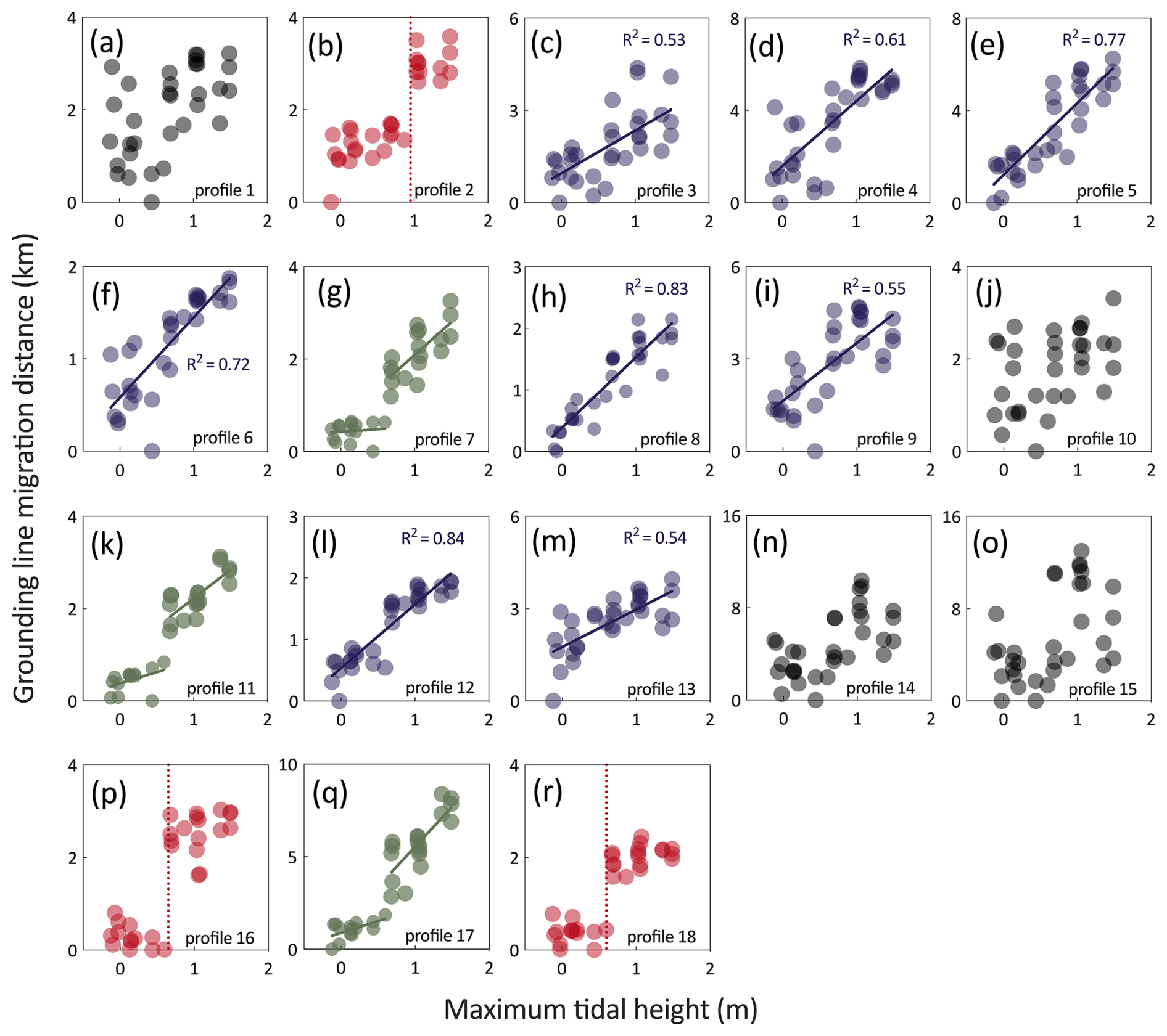
Figure 4 Tidal GL migration modes of AmIS. The label in the lower right corner of each subplot indicates the corresponding profile number, consistent with the profile numbering in Figure 1b. The relationship between GL migration distance and maximum tidal height is depicted across different modes: Threshold (subplots with red points represent profiles where a threshold relationship is observed between GL migration and maximum tidal height. The red dashed line indicates the threshold beyond which significant GL migration occurs), Linear (subplots with purple points show a linear relationship between GL migration and maximum tidal height, with the purple solid line representing the best-fit linear regression), Asymmetric (subplots with green points display an asymmetric relationship, with two green solid lines representing the linear fits for different ranges of maximum tidal height), and no clear mode (subplots with black points indicate profiles where no clear mode is observed between GL migration and maximum tidal height). Note that a GL migration distance of 0 km represents the location of the seawardmost GL observed in each profile, which is used as the reference point for calculating relative migration distances.

While most GL migration shows a correlation with tidal height, as illustrated by Fig. 4, the migration patterns of the remaining four profiles (1, 10, 14, and 15) do not follow this trend (Fig. 4a, j, n, and o). In these cases, GL migration does not exhibit a clear relationship with maximum tidal height, and sometimes even demonstrates greater upstream migration during lower tides. This discrepancy could be explained by some studies which suggest that a linear relationship between GL position changes and tidal height only holds when tidal height approaches infinity (Tsai and Gudmundsson, 2015). In the AmIS, the tide range is approximately between −1.2 and 1.6 m, but the range captured from SAR images in 2021 spans from −0.4 to 1.5 m, covering only 64 % of the full tidal cycle. Therefore, when tidal height are not sufficiently extreme, other factors, such as basal properties, surface slope, and ice thickness, may play a more significant role in affecting the ephemeral migration of the GL. Furthermore, similar to the DDInSAR technique, DROT captures a tide range rather than a specific tidal height. Using the maximum tidal height from the selected SAR images for discussing the relationship between the tide range and ephemeral GL migration may not provide a comprehensive insight, therefore, we investigated the relationship between double-differential tide range and the GL positions (Fig. S4). We find that there is a positive linear relationship between the temporal migration distances of the GL and the absolute double-differential tide range, meaning that greater ice surface deformation corresponds to a more inland position. Here, the double-differential tide range refers to the absolute difference in ocean tide height change between two ROT pairs used in DROT processing. Each ROT result is computed from a SAR image pair and reflects the ice deformation induced by tidal forcing during that interval. The double-differential range therefore approximates the variation in tidal height between two measurement periods. While this metric does not fully capture the cumulative tidal forcing or ice deformation. For instance, if both ROT pairs are acquired during similar tidal stages (e.g., both from low to high tide), the double-differential range may appear small, even though substantial ice deformation occurs within each pair. Despite this limitation, we observe a general trend that greater double-differential ranges are associated with broader GL migration, suggesting that short-term variability in tidal forcing plays a significant role in modulating the observed GL positions. So far, there is no definitive conclusion as to whether the maximum tidal height or the double-differential tide range predominately influences the GL migration when it comes to double-differential methods (DROT and DDInSAR). The results of our study indicate that along these profiles there are different migration modes in relation to the maximum tidal height, whereas a linear trend is observed when considering the absolute double-differential tide range.

3.4 Regional Case Studies

3.4.1 Case A: The widest grounding zone observed in Amery Ice Shelf

Spatial analysis of the GZs on the AmIS reveals significant variation in the GZ width, with the widest section reaching 14.2 km upstream of its most seaward limit (box A in Fig. 1a). Unlike the linear, asymmetric, and threshold modes of tidal GL migration previously outlined, profiles 14 and 15 (Fig. 4n and o) do not follow these patterns, with no clear link between absolute GL positions and the maximum tidal height observed over the study period. This finding challenges our hypothesis that the most retreated GL positions correlate with the highest tides. Both profiles 14 and 15 lack a migration pattern that correlates with the ocean tides, which aligns with the findings of Chen et al. (2023) who report a recurring pattern where the GL alternates between two positions. After the GL stabilizes upstream for several weeks, it then transits downstream. These re-advances do not correlate with tide cycles, and the transitions do not coincide with periods of lower tides. However, the simultaneous occurrence of these shifts in both profiles 14 and 15 suggests a more complex interplay with tidal states than direct causation. We studied profiles 14 and 15 during different tide states over time, which revealed a consistent downstream migration of 7 km over the initial three months of our study period (31 January to 25 April 2021), a nearly six-month stabilization near this new position, followed by a swift retreat to the starting location within a month (Fig. 5b). This apparent switching behaviour between discrete GL positions is consistent with previous findings (Chen et al., 2023), which documented similar bistable GL states at Lambert and Mellor Glaciers over multi-month timescales. Due to the lower temporal sampling in our study compared to Chen et al. (2023), some short-term or transitional events may not have been fully captured. As a result, the discrete nature of the observed GL states may partly reflect our sampling interval. Nevertheless, the persistence of these states across successive observations suggests a degree of stability in the GL position under specific tidal or stress conditions.

Considering that three major glaciers that converge in area A, the dynamic changes of these glaciers will directly affect the grounding zone in this region (Fig. 5a). A chain of active lakes was discovered beneath Lambert Glacier with isolated subglacial lakes are thought to exist in the upstream regions of the Mellor and Fisher Glaciers and areas where the ice flow is relatively slow (Wearing et al., 2024). While subglacial hydrological pathways are known to exist at the ice-bed interface, active subglacial lakes intermittently fill and drain, substantially altering the subglacial water pressure. When active subglacial lakes drain, they release large quantities of water, increasing the water pressure at the ice-bed interface. This elevated pressure reduces friction between the ice and its bedrock, effectively lubricating the ice base, which can increase the velocity of ice flow towards the ocean. When cold, fresh subglacial water enters the ocean at the grounding line, it can cause plume driven turbulent melt at the ice shelf base, thinning the ice shelf in the vicinity of the GL or producing smaller scale channelized melt features (Gwyther et al., 2023; Nakayama et al., 2021). Drainage of large volumes of water from active subglacial lakes may lead to the formation of efficient subglacial channels that transport meltwater from the interior of the continent to the GLs. These channels can deliver relatively warm water (warmer compared to the surrounding ice) directly to the ice shelf base (Goldberg et al., 2023), which can enhance basal melting by increasing the heat flux at the base of the ice shelf. Enhanced basal melting can thin the ice shelf and potentially destabilize it over time. The previous study (Adusumilli et al., 2020) elaborates on spatially averaged melt rates for AmIS, where rates varied from near zero to 6.5 m yr⁻¹, with maximum values observed between 2003 and 2007. This variability in melt rates is speculated to be linked to the drainage of a ∼ 0.8 km³ subglacial lake under Lambert Glacier, which can drive energetic plumes that increase basal melting rates near GLs. These observations highlight the importance of considering subglacial hydrological processes and their potential to influence GL stability beyond direct tidal interactions. The recurring, non-cyclic GL migration observed in profiles 14 and 15 could be partly explained by subglacial water fluxes that impact the GL position independently of tidal forcing, further emphasizing the complex drivers of GL dynamics in AmIS.

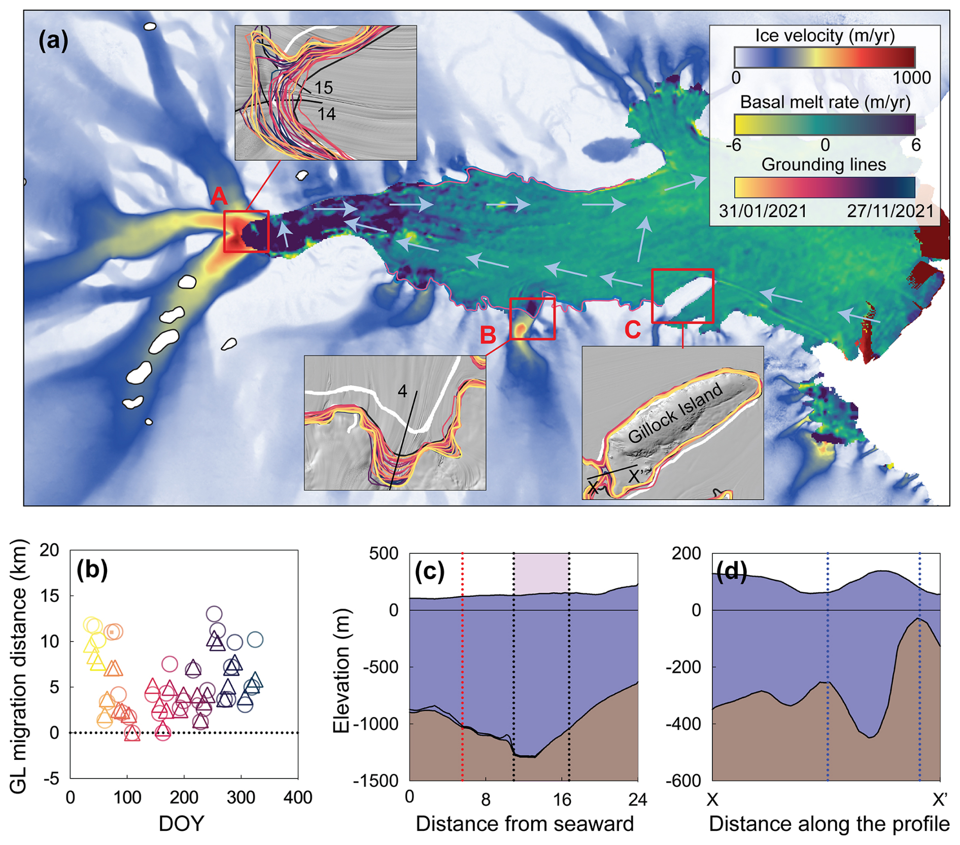
Figure 5 (a) Map showing basal melt rates (Davison et al., 2023) and ice velocity (Rignot et al., 2017) across AmIS, with zoomed-in views of three key regions (A, B and C) highlighted in the main map with red boxes. The coloured lines represent DROT-derived GLs at 32 dates, while the white line indicates the GL from MAGLv2 dataset (Rignot et al., 2016). The light blue arrows represent the likely clockwise direction of ocean water circulation within the AmIS cavity. (b) Time series plot showing GL migration distance along two profiles (shown in zoomed-in maps of region A), where circles represent profile 14 and triangles represent profile 15. The colours correspond to those used in (a). (c) Elevation along profile 4 (shown in zoomed-in maps of region B), with the red dashed line indicating the GL from MAGLv2 and the purple shading between the two dashed lines representing the DROT-derived GZ in this study. (d) Elevation along the transect X–X' (shown in zoomed-in maps of region C), with the blue dashed line outlining the region between Gillock Island and the ice sheet, showing the sector's vertical structure. All elevation data are sourced from the MEaSUREs BedMachine Antarctica Version 3 (Morlighem, 2022).

The absence of permanent GL retreat at area A, despite its relatively high basal melt, can be attributed to several factors. The basal melt of area A is driven by cold, dense high salinity shelf water and typically involves refreezing of some of the meltwater back onto the ice shelf, which can mitigate direct contributions to sea level rise by maintaining a sort of balance at the GL (Adusumilli et al., 2020; Jacobs et al., 1992; Motyka et al., 2013; Smith et al., 2009; Washam et al., 2019). In the case of the AmIS, about a fifth of the meltwater generated from basal melting is refrozen as marine ice, which contributes to maintaining the stability of the GL. It is precisely because the ice near the GZ undergoes a cyclical process of melting, freezing, and remelting that the GL position may continuously change. The greater the ice shelf basal melt rate the more significant the impact on this area is likely to be, and consequently, the larger the extent of the GZ becomes.

3.4.2 Case B: Long-term Grounding Line Retreat

Long-term GL migration is crucial for predicting the stability of ice sheets and their impact on global sea level rise. It serves as a key indicator of the interactions between climate change and polar ice dynamics. Research on the AmIS since 2000 has concentrated on understanding its mass balance, surface meltwater (Tuckett et al., 2021), ocean circulation beneath the ice shelf (Wu et al., 2021), thermal structure and stability (Wang et al., 2022), and the effects of iceberg calving and basal melting (Walker et al., 2021). However, studies focusing specifically on the dynamics of the GL of the AmIS are relatively scarce. This indicates a potential gap in the literature where more focused studies could enhance our understanding of GL behaviours in relation to broader climatic and oceanic influences. Here, we bridge this gap by comparing our DROT-derived GL which is based on Sentinel-1 images from 2021, to the composite MAGLv2, which, in the AmIS region was derived from RADARSAT images acquired in 2000. Our comparative analysis reveals a significant retreat of the GL in area B (Fig. 5c), with the maximum retreat reaching up to 5 km compared to the seaward DROT-derived GL and 10 km compared to the landward DROT-derived GL. This observed GL retreat in area B may be significantly influenced by high basal melt rates. The AmIS experiences elevated basal melt rates in specific regions, particularly along profile 4 (Fig. 5a), where average melt rates are reported at 8.3 m yr⁻¹ (Davison et al., 2023). This high melt rate likely contributes to GL retreat by thinning the ice shelf, which reduces buttressing and promotes imbalance near the GZ. Several oceanic models have confirmed a clockwise circulation within the AmIS ice cavity (Herraiz-Borreguero et al., 2015; Liu et al., 2018), moving from east to west (the light blue arrows in Fig. 5a) through Prydz Gyre. The basal melting is further influenced by the inflow of warm modified Circumpolar Deep Water on the eastern side of the AmIS, contributing to increased basal melting on the eastern AmIS, reducing ice shelf thickness, and thus promoting GL retreat.

In addition to basal melting, the observed GL retreat in this region may be influenced by the drainage of supraglacial lakes. Widespread supraglacial lake networks have been documented up to 30 km upstream of the GZ in this region, and satellite observations show that they have reoccurred up to 14 times between 2005 and 2020, suggesting consistent seasonal surface melt (Tuckett et al., 2021). On grounded ice, lakes commonly develop in areas with localized melt enhancement and relatively low accumulation rates, often located near rock outcrops and blue ice. The regular formation of surface lakes in the same location each year over decades indicates that surface melt is a persistent factor in the region's glaciological environment, with potential implications for ice flow and other ice dynamic parameters such as the GL (Kingslake et al., 2017; Langley et al., 2016). When supraglacial lakes drain, potentially through processes such as hydrofracturing, meltwater released may lubricate the glacier bed, accelerating ice flow and possibly impacting the GL location.

The retreat of GLs is also significantly influenced by whether the underlying bed slope is retrograde or prograde (Joughin et al., 2014; Schmidt et al., 2023; Schoof, 2007). Along the GL retreating path, the underlying bed slope of the first half is in a retrograde state (Fig. 5c). As the ice retreats into deeper water, more of the ice shelf lifts off the bed and becomes afloat, reducing frictional resistance and promoting further retreat. However, in the latter half, to the south, it slopes upward as it extends inland from the GL, which generally offers more stability, slowing down GL retreat and providing a buffer against rapid changes.

3.4.3 Case C: Intermittent Grounding

Our observations have identified an anomalous peninsula of the AmIS coastline situated between Gillock Island and the ice sheet, where we observe relatively short-term transitions between grounded and ungrounded states. Published GL datasets, like the MAGLv2 and Synthesized GL, have consistently shown this area as grounded; however, our DROT-derived data from 2021 definitively shows that the region is both grounded and ungrounded at different time periods. For example, our results show that between 31 January and 24 April 2021 the region is ungrounded, between 19 May  and 6 June 2021 the region is grounded, and then between 12 and 30 June 2021 the region is ungrounded again. This cyclical behaviour is atypical for Antarctic coastline regions and might be influenced by the subglacial topography and oceanographic dynamics. Bed topography data (Morlighem, 2022) show that a 447 m deep trough is present at the “neck” of the peninsula (Fig. 5d), which could channel warmer ocean water that may enhance basal melt rates. This process intermittently reduces the ice's grounding, leading to periods where Gillock Island acts as an isolated pinning point. While basal melt variability provides one plausible explanation, it is important to consider ocean tides as an additional factor influencing grounding. Tidal fluctuations may cause periodic changes in water pressure beneath the ice shelf, which can alternately ground and unground regions close to the threshold of flotation (Padman et al., 2018; Rignot et al., 2011). During high tides, buoyant forces could lift the ice, causing ungrounding, while low tides might allow the ice to settle back onto the bedrock. This tidal influence, especially near regions with topographic lows (Fig. 5d), can significantly impact GL dynamics and might work in tandem with basal melting to drive the observed oscillatory grounding behaviour (Gudmundsson, 2011; Robel et al., 2017). Such observations underscore the complexity of ice sheet dynamics and emphasize the influence of subglacial and oceanographic features in determining the stability and response of ice structures in polar environments. Incorrect determination of the GL is important as it could lead to inaccuracies in models predictions of ice dynamic behavior, which are essential for forecasting sea level rise (Andrew et al., 2018; Rignot et al., 2014).

4 Discussion

4.1 Advantages and Limitations of the DROT Method for Monitoring Grounding Line Migration

The prevalent remote sensing methods for investigating the temporal migration of GL positions primarily include RTLA which is based on ICESat and ICESat-2 datasets, and DDInSAR, which utilizes SAR imagery. In comparison to RTLA, the DROT method used in this work has the advantage that it has (i) all-weather measurement capability as SAR images penetrate through cloud cover and precipitation, enabling effective operation under poor weather conditions that would typically impede laser altimetry; (ii) higher spatial resolution although RTLA has a finer along-track resolution of 20 m (Freer et al., 2023) compared to DROT's 100 m (Wallis et al., 2024), DROT offers a more continuous spatial measurement, as RTLA has data gaps every 2.8 km due to the track spacing (Abdalati et al., 2010). This enables DROT to capture fine-scale GL features across larger areas without interruption. Finally, (iii) DROT GL measurements can be made at fine temporal resolution every 6 to 12 d vs. the typical 91 d repeat period for laser altimetry missions, providing more frequent and continuous temporal coverage which is essential for monitoring short-term tidally induced GL migration. The DDInSAR technique shares many of the advantages of DROT outlined above, however, its requirement for high coherence which can be easily lost, limits the extent to which this method can be used. Coherence is reduced if the scattering properties of the measured surface are not stable between two subsequent acquisitions, which frequently takes place due to snow deposition, snow redistribution or surface melt, as well as due to fast ice flow. The main benefit of DROT over DDInSAR is the ability to apply this technique in low-coherence areas.

A limitation of the DROT method is that unlike RTLA the DROT method cannot detect the GL position at a specific time point but instead measures the location within the tide range that occurs between two image acquisition dates. Prior to the launch of Sentinel-1 in late 2014 SAR images were not routinely acquired over the whole Antarctic coastline limiting the ability to apply techniques such as DDInSAR or DROT that require these input datasets. In contrast, altimetry missions such as ICESat-2's have an orbit covers the entire Antarctic coastline yielding a more comprehensive spatial coverage, even if the spatial resolution is coarser. As new SAR missions such as the NASA-ISRO NISAR and ESA-Copernicus ROSE-L missions are launched, this will add to the volume of SAR data already acquired by Sentinel-1, ensuring excellent spatial and temporal coverage. All tidally sensitive GL measurement techniques perform best in regions with a high tidal difference, where the boundary between floating and grounded ice is more easily distinguished above any measurement noise. The DDInSAR and RTLA techniques have more sensitivity to vertical displacement of the ice surface than the DROT technique, however, there is also a range of performance for the DROT method when applied to different radar frequency SAR data, with shorter wavelengths (e.g. X-band SAR) having more sensitivity to the altitude of ambiguity than longer wavelength (e.g. C-band SAR). The most significant limitation of DROT is the inability to distinguish between actual tidal and non-tidal-driven velocity variations, and the artificial tidal bias. Non-tidal-driven velocity variations refer to changes in ice flow speed that are not caused by tidal forces, such as seasonal changes in ice dynamics, subglacial water drainage, or adjustments in ice shelf stress. This artificial tidal bias arises from vertical displacement of the ice shelf due to tidal lifting and lowering, which, when measured by satellite radar, appear as horizontal movements along the radar's ling of sight. Since DROT can only track movement in the direction of the radar signal, these vertical shifts are misinterpreted as horizontal migration of the GL, even though they are not true horizontal movements caused by tidal forces. This projection effect can lead to errors or distortions in the results, potentially causing misinterpretations about the true position and movement of GL (Friedl et al., 2020).

4.2 Potential for Measuring Pinning Points

A significant amount of ice loss from the Antarctic Ice Sheet can be attributed to the effects of warm ocean currents undermining the buttressing capability of ice shelves, leading to their thinning and increased basal melt (Jenkins et al., 2010, 2018; Pritchard et al., 2012). This process has direct implications for the acceleration of ice discharge into the ocean (Greene et al., 2022; Gudmundsson et al., 2019). Therefore, comprehensive observations that monitor the changes in ice-shelf properties are crucial for understanding the evolution of the Antarctic Ice Sheet and for predicting future patterns of ice loss. Changes in the surface expression of pinning points, as a proxy for ice-shelf thickness change, could assist in reducing uncertainties regarding Antarctica's impact on global sea level (Edwards et al., 2019; Miles and Bingham, 2024; Ritz et al., 2015). Pinning points are locally grounded features on ice shelves that provide additional buttressing to the ice flow (Matsuoka et al., 2015). They are regions where the ice shelf is anchored to the bedrock or underlying topography, providing structural stability to the shelf and resisting the flow of ice (Jenkins et al., 2010; Roberts et al., 2018). Larger pinning points provide more substantial buttressing against the flow and bending of ice shelves, thereby slowing down the ice flow and enhancing stability. Their presence can influence the pattern of ocean circulation beneath the ice shelf, which, in turn, affects the basal melting patterns. Moreover, large pinning points can cause the ice flow to diverge around them, creating complex flow structures within the ice shelf. Consequently, understanding the role of pinning points and measuring any change in their area helps to assess the stability of ice shelves and the potential for rapid ice-sheet changes.

Figure 1c clearly showcases the potential of the DROT technique for measuring ice shelf pinning points in the AmIS, including their location, area, and grounding conditions during various tidal states. Our findings show that DROT results can be used to identify 11 pinning points on the AmIS (labelled a-k according to the direction of ice flow in Fig. 1c), including 6 new features which are not included in the MAGLv2 dataset. The occurrence of pinning point g is unstable; as discussed in Sect. 4.1, the intermittent grounding between Gillock Island and the ice shelf causes it to switch between connected and disconnected states with the ice sheet. The absence of pinning points h to k in the DDInSAR GL data product is unknown, but may be due to their location near the ice shelf edge which may have made them more difficult to identify in the interferograms. Another possibility is that the coverage of historical SAR datasets in this region was poor, leading to a more limited number of coherent InSAR, making it less likely that the pinning points were identified. Compared with other updated datasets of pinning points, some of these pinning points have been identified (Fig. S7). For example, we note that in the more recent DDInSAR GL dataset (Mohajerani et al., 2021) these pining points (f, g, h, and j) were identified, but pinning points (e, i, and k) were not. The latest optical imagery-based pinning points dataset (Miles and Bingham, 2024) successfully captured pinning points (h, i, j, and k), but missed pinning points (a, c, f, and g). This suggests that when more data and automated techniques are combined, lesser studied features are identified. In addition to mapping the number of pinning points, our DROT results allow us to measure the pinning point area over time and at different tidal states. For example, the area of pinning point “a” fluctuates between 170 and 289 km² in the 32 DROT results we sampled. Summing up all 11 pinning points within the AmIS, their combined minimum area totals 639 km², while the maximum combined area reaches 956 km². The size of pinning points has a direct impact on their buttressing influence therefore understanding how pinning point area varies over time will be important for modelling studies. In summary, the DROT results effectively identify the locations and areas of ice shelf pinning points, and there is an opportunity for future studies to use this technique to monitor pinning points on ice shelves across Antarctica.

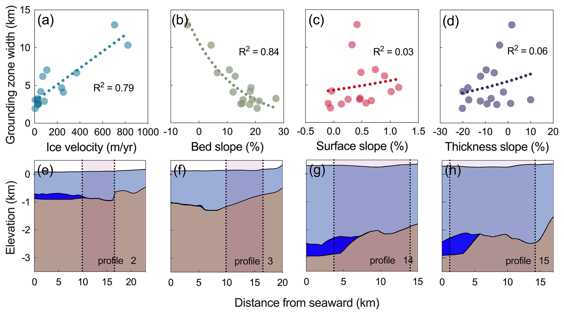
Figure 6 The top row (a–d) shows the correlation between GZ width and various glaciological parameters: (a) ice velocity (sourced from the MEaSUREs InSAR-Based Antarctica Ice Velocity Map, Version2 (Rignot et al., 2017)), (b) bed slope, (c) surface slope, and (d) ice thickness slope, all derived from the MEaSUREs BedMachine Antarctica Version 3 (Morlighem, 2022). The R² values indicate the strength of these correlations. The bottom row (e–h) presents the cross-sectional elevation profiles corresponding to profiles 2, 3, 14, and 15, with data soured from the MEaSUREs BedMachine Antarctica Version 3. The GZs marked by the shaded areas between the dashed lines. The slopes used in panels (b)–(d) were calculated by linearly fitting the respective data over the domain bounded by the black dashed lines in panels (e)–(h), which represent the landward and seaward limits of the tidally-induced short-term GL migration.

4.3 Factors Affecting the Grounding Zone Width

As illustrated in Fig. 1c, the GZ of AmIS exhibits varying widths depending on the coastal geometry. In areas with a smooth, straight coastline, like profile 1 and 2 (Figs. 1b and 2a–b), the GZ is narrower, typically less than 4 km. Conversely, in regions with indentations or more constricted coastal features, such as profiles 4, 14, and 15 (Figs. 1b and 2d, n, and o), the GZ becomes wider. We note that these confined regions tend to cluster in areas of ice stream convergence or where the ice velocity is higher. Therefore, we compare the GZ width along the profile direction with the average ice flow velocity (Fig. 6a), and the results indicate a linear relationship; the greater the ice flow speed, the larger the GZ width. The specific geometry of an ice shelf and its interconnection with the inland ice also significantly impacts its tidal response. Areas where the ice shelf curves towards the ice sheet have a different stress distribution, leading to a more varied tidal response compared to more linear sections (Brunt et al., 2010). Faster ice flow suggests higher dynamism in that region, potentially leading to a more sensitive response to external forces like tidal motion. Areas with rapid ice flow may experience greater stress concentration, making the ice shelf more prone to deformation under tidal forces. There can be complex interactions between the dynamics of ice flow and tidal forces, leading to more pronounced tidal responses in areas of faster ice flow (Brunt et al., 2010).

Our study involves a comprehensive evaluation of the relationship between GZ width and the corresponding slopes of the bedrock (Fig. 6b), surface (Fig. 6c), and ice thickness (Fig. 6d). In areas with a wide GZ, we observe that the bed slope typically exhibits either a retrograde or a mild prograde inclination. This is especially evident in profiles 14 (Fig. 6g) and 15 (Fig. 6h), where the seawater, upon traversing the initially gentle prograde slopes of the bedrock, progresses into an extensive area of retrograde slopes measuring several km in length, with slopes of 4.1 % and 1.4 % respectively. Conversely, for the majority of the profiles studied the seawater's forward motion is hindered by more pronounced prograde slopes at the onset, which exhibit steep inclines of between 21 % to 61 %. This suggests that the geometry of the initial bedrock incline plays a pivotal role in influencing the extent of seawater penetration into the GZ. To quantify the slopes associated with the GZ width, we have adopted a method of averaging the slopes located seaward and landward of the GL. The result indicates a quasi-exponential relationship between the GZ width and the bed slopes (Fig. 6b), indicating that as the bed slope becomes gentler, the GZ width tends to expand significantly. Notably, however, this correlation does not extend to the surface slope or ice thickness slope. Our analysis does not reveal any obvious mathematical relationship between these parameters and GZ width, suggesting that other factors or complex interactions may govern the influence of surface and ice thickness slopes on GZ width. This absence of a clear link highlights the need for further research to understand the interplay of these variables and the dynamics of GZ stability and migration.

5 Conclusion

Our study has used the DROT technique to measure the short-term migration of the GL under the influence of tidal variations on AmIS. We used the DROT method to observe GL positions at different tidal states throughout 2021 producing a comprehensive map of the GZ distribution across the ice shelf, which fluctuated significantly in response to tides ranging from −0.5 to 1.5 m. Our results perform well compared to the contemporaneous DDInSAR measurements, with a mean seaward separation between these data of 0.37 km and a standard deviation of 0.19 km. We analyse our results to show three different modes of GL migration, (linear, asymmetric, and threshold), in relation to the maximum tidal height, and we show there is a positive linear trend when considering the absolute double-difference tide range. Our results show that beyond ocean tide driven variability, factors such as basal melting, subglacial topography, and ice flow velocity play significant roles in influencing GL migration patterns. These findings reveal localized variations in GL behavior, including evidence of long-term GL retreat of 5 to 10 km in area B (Fig. 5) of AmIS, highlighting the complex interplay of environmental and glaciological factors on GL stability and migration. In addition, we found that the DROT technique can be used to accurately identify the location and area of ice shelf pinning points, which could be used a proxy for ice-shelf thickness change. Looking forward, studies should extend the application of the DROT technique across Antarctica, and combine these results with other remote sensing techniques to enrich the dataset available for studying the Antarctic grounding zone. Only through a multifaceted approach can we hope to gain a holistic understanding of the processes governing the GZ and, by extension, the health of the entire Antarctic Ice Shelf system.