the Creative Commons Attribution 4.0 License.
the Creative Commons Attribution 4.0 License.
 | 16 Sep 2025
Sub-shelf melt pattern and ice sheet mass loss governed by meltwater flow below ice shelves
Erwin Lambert
Roderik S. W. van de Wal
Ocean-induced sub-shelf melt is one of the main drivers of Antarctic mass loss. Capturing it in ice sheet models is typically done by using parameterisations that compute sub-shelf melt rates based on local thermal forcing. However, these parameterisations do not resolve the 2D horizontal flow of the meltwater layer, either neglecting it entirely or simplifying its representation. In this study, we present a coupled setup between the ice sheet model IMAU-ICE and the sub-shelf melt model LADDIE. LADDIE resolves 2D horizontal meltwater flow beneath an ice shelf, incorporating both topographic steering and Coriolis deflection of meltwater plumes. We conduct simulations in a framework closely resembling the Marine Ice Sheet Model Intercomparison Project third phase (MISMIP+), which represents an idealised ice-sheet–shelf system. Simulations using LADDIE to calculate melt rates reveal key differences compared to simulations using the widely adopted sub-shelf melt parameterisations. These differences primarily emerge as variations in timing, location, and persistence of strong melting, leading to distinct transient volume loss. In the LADDIE experiments, a stepwise increase in ocean temperatures induces an initial steepening of the ice draft near the grounding line. This strengthens the westward flow, which converges into a western boundary channel, leading to persistent strong melting along the western margin. Consequently, western margin thinning results in reduced buttressing and strong volume loss over the first 300 years of the simulations. Over longer timescales, a weakened meltwater flow circulation due to reduced thermal forcing at the grounding line allows the western margin to thicken again, suppressing volume loss. In contrast, the parameterisations' limitations in representing the 2D horizontal meltwater flow prevent these experiments from capturing the influence of ice draft steepening on enhanced margin melt. This results in a different transient volume loss between the parameterisations and LADDIE. Compared to LADDIE, the parameterisations either inherently overestimate the persistence of margin thinning, leading to a sustained strong volume loss, or they underestimate margin thinning, delaying the onset of strong volume loss. Our findings suggest that incorporating the more detailed melt patterns resulting from the 2D horizontal meltwater flow in ice sheet models could significantly alter projections of Antarctic ice sheet evolution compared to melt patterns computed by the currently more common parameterisations.
- Article
(8754 KB) - Full-text XML
-
Supplement
(9168 KB) - BibTeX
- EndNote


The Antarctic ice sheet has been losing mass at an accelerating pace over the last 3 decades, increasing its contribution to sea level rise (Fox-Kemper et al., 2021; Otosaka et al., 2023). This mass loss is modulated by surrounding ice shelves that buttress the ice flow (Gudmundsson, 2013). Satellite observations indicate a rapid thinning of these ice shelves (Adusumilli et al., 2020; Davison et al., 2023), driven by the enhanced intrusion of warm ocean water into ice shelf cavities causing increased sub-shelf melt (Jenkins et al., 2018). The reduction in ice shelf thickness weakens the buttressing effect, resulting in increased ice discharge from outlet glaciers at the ice sheet margins (Paolo et al., 2015; Rignot et al., 2019). This makes ocean-induced sub-shelf melt one of the main drivers of current Antarctic mass loss (Pritchard et al., 2012; Gudmundsson et al., 2019).
Sub-shelf melting occurs in highly heterogeneous patterns, typically exhibiting higher melt rates near the grounding line and in basal channels due to topographic steering of meltwater plumes (Rignot and Jacobs, 2002; Alley et al., 2016; Berger et al., 2017). Warm ocean water, which is dense and saline, enters the ice shelf cavity and comes into contact with the ice shelf base. Here, meltwater is formed and transported along the ice shelf base before exiting the cavity at the ice shelf front, thereby forming a meltwater layer below the ice shelf (Jenkins, 1991). The interaction between the meltwater flow and the topographic features of the ice shelf base enhances the spatial variability in melt rates, causing certain areas of the ice shelf to thin more rapidly. This local thinning can lead to breakthroughs and collapse of sections of the ice shelf (Alley et al., 2016; Lhermitte et al., 2020; Wearing et al., 2021). Moreover, the distribution of the melt affects the dynamic ice sheet response, with melt along shear margins inducing a greater decrease in buttressing and a stronger volume loss compared to when the same melt rates are applied along the central flow line (Jordan et al., 2018; Reese et al., 2018b).
One approach to calculate sub-shelf melt to force ice sheet models involves using 3D cavity-resolving ocean models. Ideally, this is implemented in a coupled setup to capture feedbacks between ice sheet and ocean, such as freshwater fluxes and cavity geometry altering the ocean circulation (De Rydt and Naughten, 2024). Various research groups have coupled ice sheet models to ocean models (Grosfeld and Sandhäger, 2004; Jordan et al., 2018; Naughten et al., 2021; Pelle et al., 2019; Seroussi et al., 2017) or integrated them into Earth system models (Smith et al., 2021; Siahaan et al., 2022). However, these simulations are computationally expensive and face challenges such as handling cavity expansion due to retreating grounding lines (Fox-Kemper et al., 2019) and bridging resolution gaps between models (Hoffman et al., 2024). As a result, most studies with ice sheet models presently rely on parameterisations to compute sub-shelf melt rates from ocean temperature and salinity profiles (Seroussi et al., 2024). These parameterisations range from a simple linear or quadratic scaling of thermal forcing (Beckmann and Goosse, 2003; Holland et al., 2008; Favier et al., 2019) to more advanced schemes that approximate an overturning circulation in the ice shelf cavity (Reese et al., 2018a; Lazeroms et al., 2018; Pelle et al., 2019), where the upper half of this overturning circulation represents the meltwater layer. While computationally efficient, these parameterisations often require recalibration to adapt to changing ocean conditions and geometries (Favier et al., 2019; Burgard et al., 2022). They also fall short in capturing features like channelised melt due to either neglecting the horizontal component of the meltwater flow or relying on oversimplified assumptions about its direction.
To improve the representation of 2D horizontal meltwater flow in sub-shelf melt patterns that serve as forcing for ice sheet models, while avoiding the high computational costs of 3D cavity-resolving ocean models, we introduce a new method: an online coupling between the 2D sub-shelf melt model LADDIE – the “one-layer Antarctic model for dynamical downscaling of ice–ocean exchanges” (Lambert et al., 2023) – and the ice sheet model IMAU-ICE (Berends et al., 2022). LADDIE uses ambient ocean temperature and salinity to resolve the 2D horizontal flow of the meltwater layer beneath the ice shelf, including Coriolis deflection and topographic steering. By resolving these processes, the model captures enhanced melt rates along the western margins and in basal channels, consistent with observations (Zinck et al., 2023).
In this study, we employ our new coupled framework within an idealised domain to examine the effects of 2D horizontal meltwater flow on an ice-sheet–shelf system (Asay-Davis et al., 2016). We analyse the feedbacks between ice shelf geometry and melt patterns, as well as their impact on transient volume loss and grounding line retreat. We compare the LADDIE experiments with experiments using three widely used sub-shelf melt parameterisations: the Quadratic parameterisation, scaling melt rates with local temperature (Favier et al., 2019); the Potsdam Ice-shelf Cavity mOdel (PICO) parameterisation, an ocean box model simulating the meltwater layer (Reese et al., 2018a); and the Plume parameterisation, describing 1D buoyant meltwater flow (Lazeroms et al., 2019). This comparison allows us to identify the feedbacks missed when 2D horizontal meltwater flow is not resolved and to assess how this affects transient volume loss. We apply two scenarios, wherein ocean conditions transition from a cold state with no melt to either moderate or warm conditions within an idealised framework. These scenarios, applied to both the LADDIE and the parameterised experiments, are used to quantify the response of the grounded ice.
The paper is organised into five sections. Section 2 outlines the model setup and experimental design. Section 3 presents our results, divided into two parts: the first focuses on the LADDIE experiments and the melt–geometry feedbacks observed when resolving 2D horizontal meltwater flow; the second examines the parameterised experiments, highlighting the key differences in terms of this feedback between melt and geometry, as well as their transient volume loss. Section 4 presents the discussion of our findings, emphasising the implications of these differences arising from resolving 2D horizontal meltwater flow compared to using the parameterisations. Finally, Sect. 5 summarises the main conclusions and recommendations.
In Sect. 2.1, we introduce the ice sheet model IMAU-ICE and the sub-shelf melt model LADDIE. Moreover, we discuss the coupling method between these models, including the coupling frequency and extrapolation methods. The coupled setup can be applied on different model domains. Section 2.2 introduces the idealised geometry considered in this study, as well as the initialisation, tuning procedure, and details of the individual experiments.
2.1 Model description and settings
2.1.1 Ice sheet model IMAU-ICE
We perform ice sheet simulations using the vertically integrated ice sheet model IMAU-ICE v2.0 (Berends et al., 2022). The setup of the model employed in this study uses the hybrid shallow-ice–shallow-shelf approximation (SIA–SSA) to compute the ice dynamics over floating and grounded parts of the ice sheet (Bueler and Brown, 2009). To improve grounding line dynamics, the model scales the basal stress with the sub-grid grounded fraction, following the approach taken by other ice sheet models, like PISM (Feldmann et al., 2014) and CISM (Leguy et al., 2021). In our study, the model is configured with a horizontal resolution of 2 km and a dynamic time step, with a lower limit of 0.01 years and an upper limit of 0.125 years. This variable temporal resolution ensures stability, while at the same time it limits computation time.
While the choice of sliding law has been shown to influence model results (Cornford et al., 2020), Berends et al. (2023), using the same ice sheet model and idealised domain as in our study, demonstrated that its impact is much smaller compared to that of the sub-shelf melt implementation. Given the focus on the latter, we conduct our experiments using a single sliding law: the Coulomb-limited modified power-law relation introduced by Schoof (2005). This choice is motivated by Joughin et al. (2019), which shows that the Coulomb-limited law best captures the dynamics at Pine Island Glacier. Furthermore, Berends et al. (2023) evaluated different methods of applying melt near the grounding line and found that the flotation criterion melt parameterisation (FCMP, e.g. Leguy et al., 2021), which applies melt only to cells meeting the flotation criterion at the centre, is least sensitive to horizontal resolution. Other methods, such as no melt (NMP) or partial melt (PMP), only converge towards FCMP as resolution increases. Based on these findings, we select the FCMP scheme for our experiments.
The standard version of IMAU-ICE includes several sub-shelf melt parameterisations which derive sub-shelf melt rates from ocean data using distinct approaches, particularly in how they represent meltwater flow. The Quadratic parameterisation uses local ocean properties at the base of the ice shelf to compute melt rates and does not account for meltwater flow (Favier et al., 2019). The PICO parameterisation is an ocean box model designed to represent the upper half of the overturning circulation within the ice shelf cavity, corresponding to the meltwater layer (Reese et al., 2018a). It simplifies the meltwater flow by assuming it is always directed from the box near the grounding line towards the box near the ice shelf front. This assumption typically leads to high melt rates in the box nearest to the grounding line and progressively lower melt rates in boxes closer to the ice shelf front. The Plume parameterisation describes the flow of a 1D buoyant meltwater plume and depends on both the local thermal forcing and the thermal forcing at the plume's origin near the grounding line (Lazeroms et al., 2018). In terms of meltwater flow representation, it identifies potential starting points for the plume along the grounding line, based on conditions such as ice shelf base slope and depth, and then assumes a straight 1D flow path from these points. Overall, none of these parameterisations capture the effects of 2D topographic steering and Coriolis deflection of the meltwater flow. Details on the implementation of these parameterisations in IMAU-ICE are given in Appendix A.
2.1.2 Sub-shelf melt model LADDIE
To improve on these built-in parameterisations in IMAU-ICE, we implemented the coupling between IMAU-ICE and the sub-shelf melt model LADDIE (Lambert et al., 2023). LADDIE models the well-mixed meltwater layer beneath the ice shelf. By modelling only this meltwater layer, LADDIE can provide sub-shelf melt fields at a spatial resolution that ice sheet models require while maintaining relatively low computational costs. The physics incorporated in LADDIE is inspired by earlier work on 2D melt plume models (Holland and Feltham, 2006). The model solves the vertically integrated Navier–Stokes equations to compute horizontal velocities, thickness, temperature, and salinity of the meltwater layer below the ice shelf. By resolving the 2D flow, LADDIE accounts for Coriolis deflection and topographic steering of the meltwater, resulting in more detailed melt patterns than the parameterisations which either neglect or approximate this flow.
LADDIE is designed to simulate steady-state sub-shelf melt rates for a given combination of ice shelf geometry and ambient ocean forcing. The model domain spans the horizontal extent of the ice shelf (Fig. 1a) and is configured with a 2 km horizontal resolution for our experiments. The upper boundary of the domain is constrained by the ice shelf draft, required as input for the model. For the lower boundary, LADDIE needs input for the ambient ocean conditions. This can be provided as vertical temperature and salinity profiles, which are then applied uniformly across the horizontal plane.
The thickness of the meltwater layer is affected by vertical exchange of volume at its horizontal interfaces. At the top of the meltwater layer, the vertical exchange of volume, heat, and salt is governed by melt or freezing. This is obtained by solving the three-equation formulation for melt and freezing (Holland and Jenkins, 1999; Jenkins et al., 2010). This formulation implies the conservation of heat and salt and additionally constrains the ice–ocean boundary to remain at the freezing point. At the bottom of the meltwater layer, the vertical exchange of volume, heat, and salt is governed by entrainment of ambient water into the meltwater layer. In our model setup, we use the Gaspar parameterisation, expressing entrainment as a function of the turbulent velocity in the meltwater layer (Gaspar, 1988; Gladish et al., 2012). This parameterisation also captures the process of negative entrainment – i.e. detrainment – allowing some of the meltwater to detach from the upper layer in regions where neutral buoyancy occurs, enabling partial separation from the ice shelf base.
At the calving front and in regions where the ice shelf melts through completely, LADDIE applies open boundary conditions between ice-covered and ice-free (i.e. open-ocean) cells. Across this boundary, the model prescribes zero gradients in all state variables – temperature, salinity, layer thickness, and horizontal velocity components. In the momentum equations, the horizontal pressure gradient force assumes a zero ice draft for ice-free cells, which drives a strong outflow of meltwater from ice-covered cells into adjacent ice-free cells. Any momentum, heat, or salt advected across this boundary is considered lost to what is treated as an infinite ocean. This effectively prevents the transfer of momentum, heat, and salt across an ice-free cell. For more detailed information on the equations and numerical aspects of the model, we refer to the model description paper (Lambert et al., 2023).
2.1.3 Coupling IMAU-ICE and LADDIE
Figure 1a shows a spatial schematic of the coupled setup between LADDIE and IMAU-ICE. At the ice–ocean interface, the models exchange ice shelf draft geometry (output IMAU-ICE, input LADDIE) and sub-shelf melt rates (output LADDIE, input IMAU-ICE). In our setup, both models use the same grid, such that no interpolation is required. Heat fluxes are coupled in one direction only (output IMAU-ICE, input LADDIE). While the meltwater layer modelled by LADDIE is affected by the ice interior temperature through the three-equation formulation, there is no sensible heat flux into the ice at the ice–ocean interface. Hence, the ice interior temperature itself is not affected by the meltwater layer.
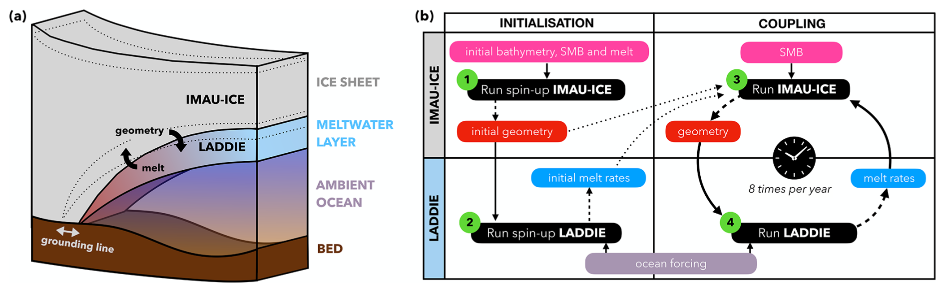
Figure 1Schematic overview of the coupled setup between IMAU-ICE and LADDIE. The spatial overview (a) shows that the models exchange geometry (draft, grounding line, and calving front position) and melt rates at the ice–ocean interface. The grounding line is allowed to retreat or advance during the simulation, which affects the horizontal extent of the LADDIE domain. The dotted lines indicate a modified IMAU-ICE geometry, featuring a retreated grounding line, and the associated adjusted boundaries of LADDIE. In the procedural overview (b), numbers indicate in which order the models run, where step 3 and 4 are repeated until the end of the simulation. The models exchange geometry and melt rates at a fixed coupling frequency (in this case eight times per year) which is independent of the time step in the individual models. Dashed arrows indicate model outputs, solid arrows indicate model inputs, and dotted lines indicate model input only used for the first time step of the coupled simulation. SMB refers to surface mass balance.
The coupled simulation procedure can be broken down into four steps (Fig. 1b). At the start of each coupled simulation, both models need to be initialised. This is done by first initialising IMAU-ICE stand-alone (step 1) and then using the resulting initial geometry, along with prescribed ocean forcing, to initialise LADDIE (step 2). Details of the initialisation settings for the coupled experiments presented in this study are provided in Sect. 2.2.1. Once initialised, the resulting geometry and associated sub-shelf melt rates are used by IMAU-ICE for the first time step of the simulation (step 3). LADDIE is subsequently run for the updated geometry (step 4). Steps 3 and 4 are repeated iteratively until the simulation ends.
The models exchange draft geometry and sub-shelf melt rates at a fixed coupling frequency. To ensure that sub-shelf melt rates are compatible with the geometry, the frequency should be picked such that changes in ice shelf geometry remain minimal over the coupling interval, specifically limiting grounding line retreat to within a single grid cell length. For the experiments conducted in this study, a frequency of eight times per year is used.
At the start of each coupling interval, LADDIE restarts using the layer thickness, temperature, salinity, and velocities from its last time step of the previous coupling interval, now taking into account the updated geometry from IMAU-ICE. When the grounding line retreats, the LADDIE domain expands accordingly, requiring the initialisation of previously grounded cells that are now floating. For the layer thickness, temperature, and salinity, the initial value is set to their nearest-neighbour average. The layer velocities in these newly floating cells are initialised at zero. The time required for LADDIE to reach a new quasi-steady state after each coupling step depends on the magnitude of changes in geometry and external forcing. Since we keep the oceanic forcing constant throughout our experiments, the adjustment time is driven solely by changes in geometry. In our setup, we found that running LADDIE for 4 d between coupling steps of 0.125 years is sufficient for the meltwater layer thickness and velocity to reach near-stable conditions.
As outlined in Sect. 2.1.1, we use the IMAU-ICE setup with the FCMP sub-shelf melt scheme. This scheme applies sub-shelf melt to grounding line cells with a floating centre. The same FCMP mask is used to constrain the ice shelf area in LADDIE. However, between coupling time steps, grounding line retreat can cause additional cells to become afloat. While the sub-shelf melt parameterisations immediately update to reflect these changes, LADDIE only updates its domain at the next coupling time step. To address this discrepancy, we use nearest-neighbour averaging to extrapolate the LADDIE melt field to include the grounding line cells. In practice, however, this extrapolation has little effect on the experiments presented in this study. The ice sheet model time step was often equal to the coupling interval, implying the extrapolated melt values are rarely applied.
2.2 Experimental settings
2.2.1 Initialisation
The ice sheet model is initialised following the MISMIP+ protocol (Asay-Davis et al., 2016). Compared to the geometry presented in the protocol paper, the coordinate system is offset by 400 km in the X direction and 40 km in the Y direction (Fig. 2). It represents a symmetric ice stream flowing into a constrained ice shelf. The spin-up runs for a total of 50 000 years until it reaches a steady state. It starts with a 100 m thick slab of ice which grows over time due to the uniform and constant surface mass balance of 0.3 m yr−1. No melt at the ice shelf base is applied during the spin-up, ensuring that the initial state is independent of how sub-shelf melting is prescribed. To obtain a stable central grounding line position at X=50 km, the spatially homogeneous flow factor is tuned throughout the spin-up. This flow factor impacts the viscosity field of the ice, consequently influencing the ice velocities. A fixed calving front is applied at X=240 km. Ice flowing across the calving front is immediately removed. We do not apply calving based on a threshold thickness. For all experiments presented in this study, we assume a constant bathymetry.
We initialise LADDIE by prescribing the initial ice sheet geometry along with the scenario-specific ocean temperature and salinity profiles. The model starts with zero layer velocities and a uniform layer thickness of 10 m. The initial temperature is set to the ambient ocean temperature at the bottom of the meltwater layer, and the initial salinity is set to 0.1 psu below the ambient ocean salinity, ensuring a stable stratification. We run the model for 40 d to obtain a quasi-steady-state melt pattern that aligns with the initial ice sheet geometry and forcing data. This timescale of 40 d is approximately twice the flushing time of the meltwater layer, which depends on both the size of the ice shelf and the oceanic forcing. This meltwater layer flushing time is considerably shorter than the flushing time of the entire cavity due to the smaller volume of the meltwater layer and the higher velocities within it (Holland, 2017). Specific parameter settings for IMAU-ICE and LADDIE are provided in Appendix B.
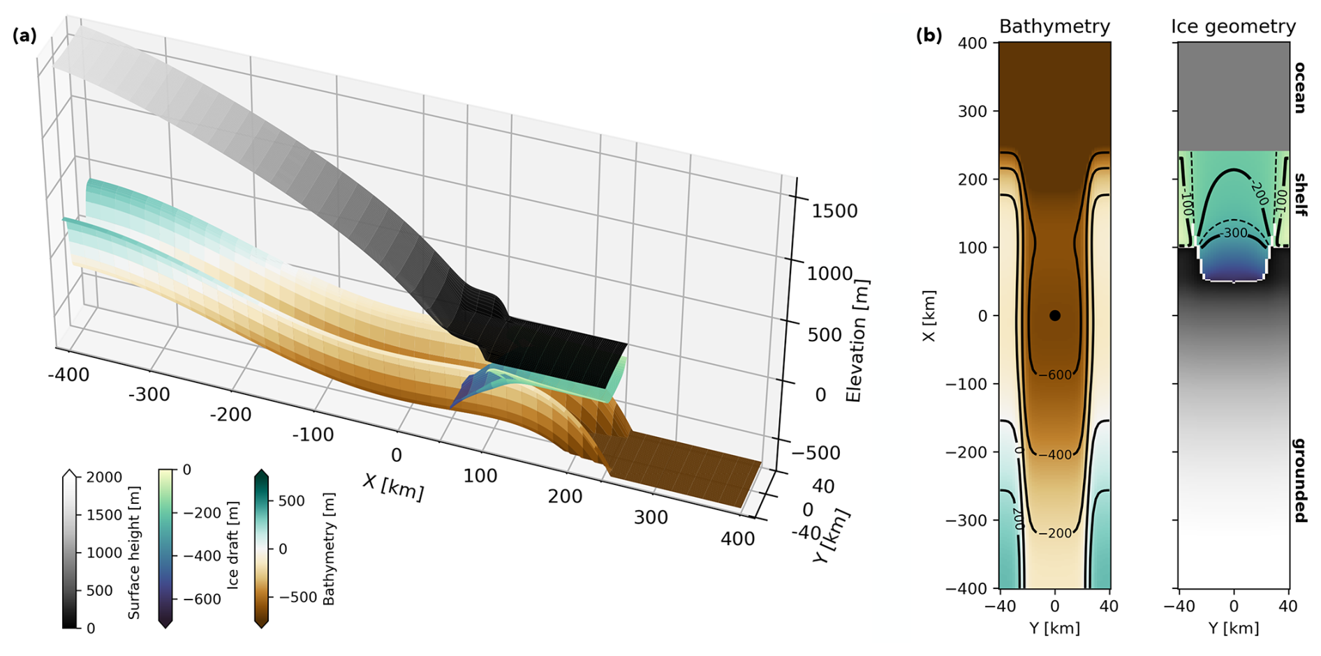
Figure 2The idealised MISMIP+ geometry, offset by 400 km in the X direction and 40 km in the Y direction with respect to the geometry presented in Asay-Davis et al. (2016). (a) 3D view of bathymetry, surface height, and ice draft. The initial grounding line is at X=50 km, and a fixed calving front is applied at X=240 km. (b) Top view of the bathymetry and the ice geometry, using the same colour scales and colour maps as in panel (a). The bathymetry top view includes contours for various depth levels, highlighting the lowest point from the initial grounding line inwards, indicated by the black dot at X=0 km. The ice geometry shows the grounding line in white and ice draft contours at levels indicated in the figure. Dashed lines represent 50 m intervals between these levels.
2.2.2 Perturbation experiments
In this study, we aim to improve the understanding of the transient response of an ice-sheet–shelf system to sub-shelf melt patterns that are governed by a 2D horizontal meltwater flow. Additionally, we compare this with the system's transient response to more idealised melt patterns derived from sub-shelf melt parameterisations. These objectives guide the selection of the perturbation experiments presented in Table 1. All simulations start from the same initial geometry (Fig. 2) and are run over a period of 1000 years. At the start of the simulations, sub-shelf melt is turned on, either through the coupling with LADDIE or through turning on one of the built-in sub-shelf melt parameterisations. We consider three such parameterisations: Quadratic, PICO, and Plume, as described in Sect. 2.1.1. In addition to the perturbation experiments, we include a “no melt” control run to evaluate model drift. This control run is solely used for drift assessment and is not employed for corrections to the perturbation experiments.
Table 1Overview of experiments. The forcing scenario relates to the prescribed temperature and salinity profiles as shown in Fig. 3.
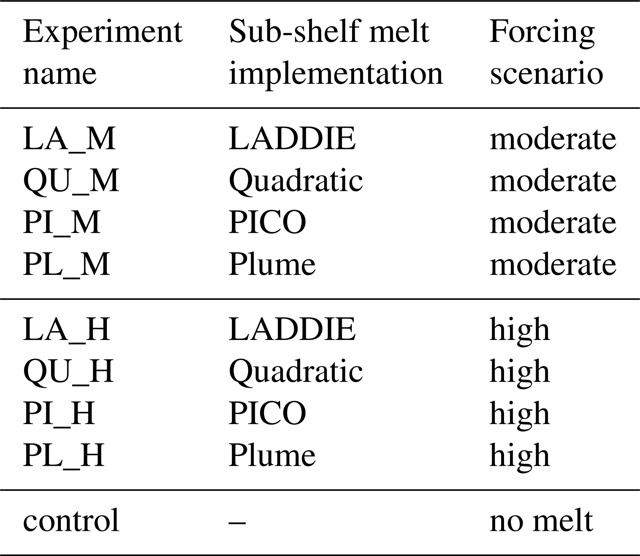
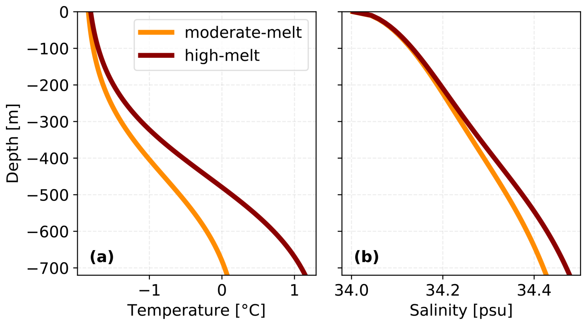
Figure 3Ambient ocean temperature (a) and salinity (b) profiles for the two forcing scenarios used in the experiments. The vertically varying profiles are uniform in horizontal space and remain constant over time.
To test the sensitivity to different ocean temperature states, we apply two forcing scenarios: a moderate-melt scenario and a high-melt scenario (Fig. 3). Both scenarios are expressed as a hyperbolic tangent profile of temperature, resembling temperature profiles observed around Dronning Maud Land and the Amundsen Sea (Locarnini et al., 2018). The salinity profiles are determined such that the density profiles of the moderate-melt and high-melt scenario are identical, based on the linear equation of state coefficients specified in Table A1. The forcing is constant over the entire duration of the simulations, allowing us to isolate the feedback between melt patterns and ice shelf geometry under steady ambient ocean conditions.
2.2.3 Tuning
To ensure a valid comparison between the simulations, we tune the heat exchange coefficient (γT) such that for the moderate-melt scenario, and based on the initial geometry, the average melt rates over the deep area of the ice shelf are consistent between LADDIE and the parameterisations. Here, we define the deep area as the area where the ice shelf draft is below −300 m (Fig. 2b), following the definition in the ISOMIP+ protocol (Asay-Davis et al., 2016).
For LADDIE, we first tune γT such that the averaged deep melt rates in the high-melt scenario are within the ISOMIP+ target of 30±1 m yr−1, determined for their WARM scenario. We then apply the resulting heat exchange coefficient to the moderate-melt scenario, resulting in averaged deep melt rates of 16.75 m yr−1. Earlier work shows that no retuning is required for LADDIE (Lambert et al., 2023), so we take the same value of γT for both forcing scenarios.
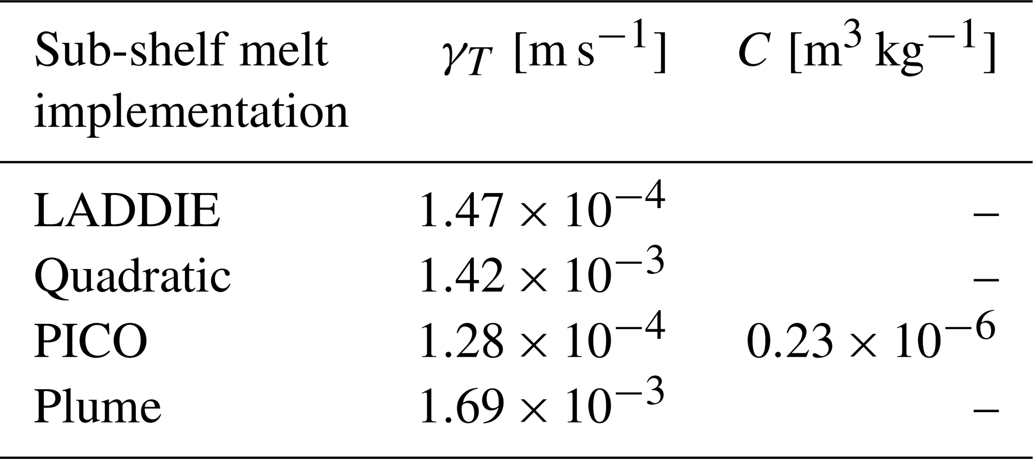
We then take the resultant averaged deep melt rates in the moderate-melt scenario to tune the parameterisations. For PICO, following Reese et al. (2023), we additionally tune the overturning coefficient (C) to optimally match the integrated melt. The values obtained from our tuning procedure are presented in Table 2.
Table 2Values of the heat exchange coefficient (γT) and overturning coefficient (C) used for tuning the different sub-shelf melt implementations.
In Sect. 3.1, we examine the feedback between sub-shelf melt pattern and ice sheet geometry for the LADDIE experiment with moderate-melt forcing (LA_M). In Sect. 3.2, we compare the LADDIE experiments with the parameterised experiments, beginning with the initial melt patterns (Sect. 3.2.1), followed by the melt–geometry feedback (Sect. 3.2.2), and concluding with the volume above flotation and grounding line retreat rates (Sect. 3.3.3).
3.1 Melt–geometry feedback in LADDIE experiments
The simulation with LADDIE melt and moderate-melt forcing (LA_M) shows a rapid grounding line retreat over the first 300 years of the simulation, initiated by high melt rates near the central grounding line and along the western shear margin (Fig. 4). The distribution of high melt rates leads to a steepening of the ice shelf base near the central grounding line. This accelerates the plume flowing along the central grounding line and the western shear margin, deepening the western boundary channel and enhancing deep melt rates. On longer timescales (600 to 800 years), the ice shelf flattens and the grounding line retreats and resides at shallower depth. As a result, the meltwater flow circulation weakens and melt rates reduce, enabling the ice shelf to stabilise on the lateral margins. In the next paragraphs, we describe this evolution in more detail.
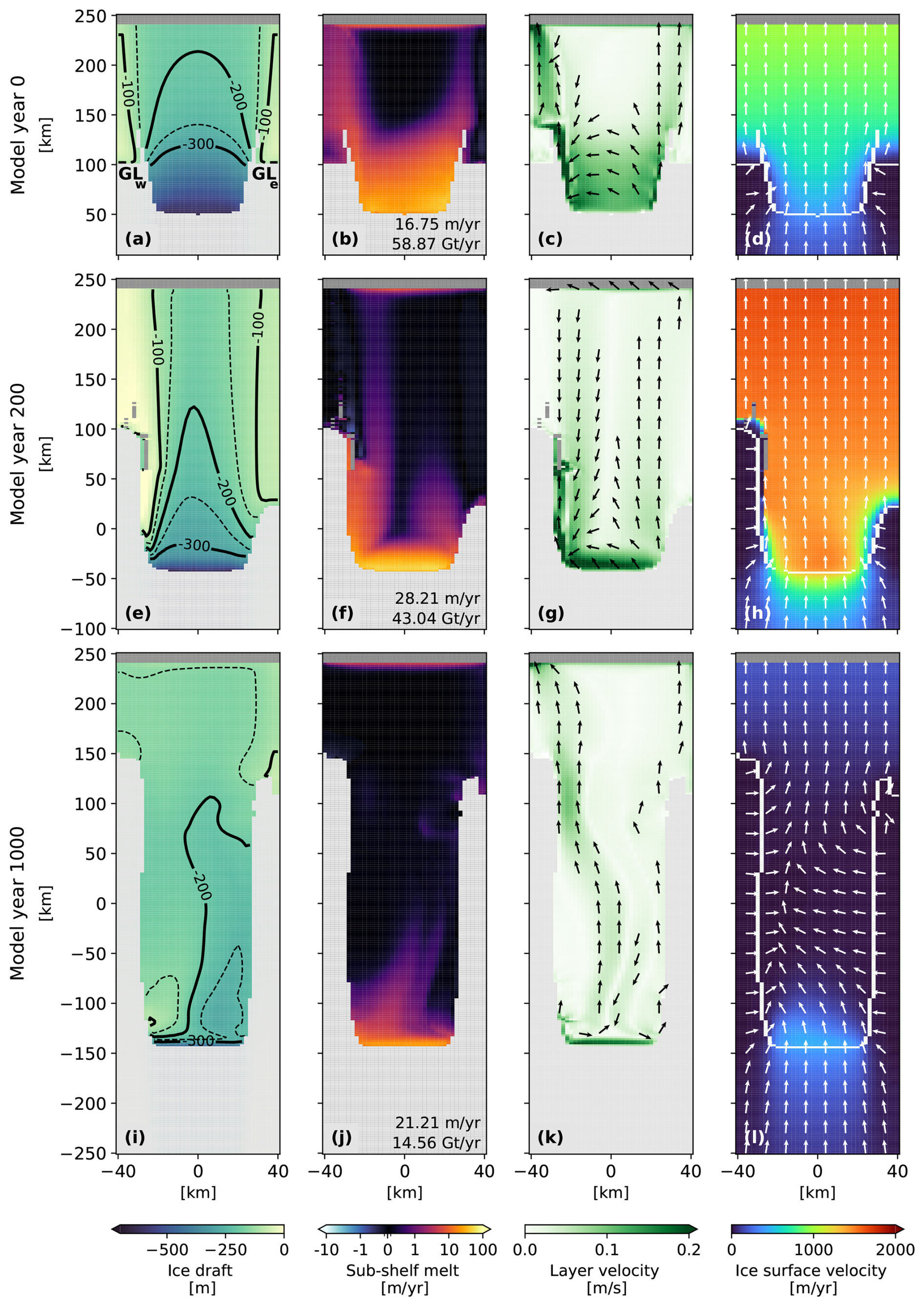
Figure 4Transient response of main variables in the LADDIE experiment with moderate-melt forcing (LA_M). The columns present the ice draft geometry, sub-shelf melt rates, meltwater layer velocities, and ice surface velocities. Contours in the first column show ice draft levels, visualised in the same manner as in Fig. 2. The averaged deep melt rates and integrated melt flux are given in the lower-right corner of the sub-shelf melt panels. In the third and fourth columns, arrows illustrate the direction of the meltwater layer velocity and ice surface velocity, respectively. Arrows for the layer velocity are omitted when velocities are below 0.02 m s−1. In the ice surface velocity plots, the grounding line is marked by a white line. Each row corresponds to a different time slice, indicated to the left of each row. The east–west-oriented grounding lines at the very edges of the domain are labelled as GLw and GLe in the upper-left panel. Grounded ice is masked in light grey in the first three columns. In all panels, the ice-free ocean is masked by dark grey. Dark-grey pixels enclosed by ice shelf pixels indicate areas of melt-through. An animation of this figure, showing time slices every 10 model years, is provided in the Video supplement.
The initial LADDIE melt pattern reveals enhanced melt rates, not only near the deep central grounding line, but also along both the shallower western and eastern flanks (Fig. 4b). The meltwater layer velocities show that, right at the grounding line, the meltwater flow rises along the ice shelf draft following the ice flow direction but then curves towards the west due to Coriolis deflection (Fig. 4c). This westward flow converges into a western boundary current which flows along the western margin of the ice shelf until it eventually reaches the ice shelf front. The boundary current leads to enhanced melt rates on the western side of the shelf, also close to the short section of the east–west-oriented grounding line at the western edge of the domain (GLw). Additionally, the meltwater layer velocities show a current originating at the eastern part of the grounding line. Guided by topographic steering, this current follows the draft contours towards the ice shelf front (Fig. 4a, c), leading to enhanced melt rates on the eastern side of the ice shelf. Melt rates near the short section of the east–west-oriented grounding line at the eastern edge of the domain (GLe) remain close to zero, however.
Over the first 200 model years, ice draft steepening near the central grounding line, driven by earlier melt patterns and accompanied by substantial retreat, increases layer velocities at this location (Fig. 4e, g). This velocity increase affects the melt pattern in two ways (Fig. 4f): first, the increase in velocity directly raises local melt rates; second, it enhances Coriolis deflection of the flow, reinforcing the western boundary channel relative to the eastern boundary channel. These combined effects concentrate high melt rates closer to the grounding line and increase deep melt rates compared to the initial state (Fig. 4b, f). Over this 200-year period, the feedback between ice draft steepening and the melt pattern becomes self-sustaining, as the enhanced melt near the grounding line maintains the steep ice shelf draft.
The reinforcement of the western current relative to the eastern current results in an asymmetry in the locations of the GLw and the GLe (Fig. 4e). The ice velocity field reveals stronger velocity gradients downstream of the GLw than those observed downstream of the GLe (Fig. 4h). Along the western shear margin and near the GLw, enhanced thinning has created a zone where the ice becomes too thin to sustain viscous flow. This effectively causes the grounded ice to dynamically detach from the floating ice, meaning that the velocities in the grounded region are isolated from the influence of the downstream floating ice. This dynamical detachment results in steep velocity gradients and near-zero velocities at the GLw, allowing it to maintain its position. In contrast, at the GLe, a smoother transition from grounded ice to floating ice enables the ice to dynamically thin and eventually unground, causing the GLe to retreat over a distance of 70 km over the first 200 years.
The persisting western boundary current causes localised melt-through along the western shear margin, as the ice flow convergence cannot compensate for the high melt rates in these areas (Fig. 4e). When the western boundary current encounters one of these areas of melt-through in the ice shelf, the buoyant plume exits the cavity through these openings. This results from the open boundary conditions imposed at the spatial interface from ice-covered to ice-free cells, as explained in Sect. 2.1.2. The areas of melt-through allow heat to escape the cavity, and the discontinuous ice shelf draft disrupts the boundary current, preventing its continuation downstream from these regions. This localised melt-through can thus serve as a negative feedback, which limits the impact of warmer forcing.
Additionally, we note that the integrated melt flux is reduced relative to the initial state (Fig. 4b, f). Both the ice shelf area and deep melt rates increased, indicating that the integrated melt over the shallower part has reduced substantially. We attribute this, first, to a larger part of the ice shelf now residing in shallower waters, where ambient ocean temperatures are colder and hence melt rates are lower. Second, we attribute it to large parts of the ice shelf becoming more flat, which suppresses layer velocities, consequently lowering melt rates.
After 1000 years, further retreat of the central grounding line leads to a reduced thermal forcing at this location, as it now resides in shallower, hence colder, waters (Fig. 4i). This results in two major changes to the melt pattern: first, it reduces melt rates near the central grounding line; second, it reduces melt along the western shear margin, as the reduced thermal forcing is insufficient to maintain the strong western boundary current (Fig. 4j). The weakened circulation, combined with topographic constraints imposed by the ice shelf draft, forces the channelised melting originating at the central grounding line to migrate eastwards (Fig. 4k). Melt rates associated with this eastward-shifted channel remain low, however (Fig. 4j). Moreover, the weaker meltwater flow, accompanied by reduced deep and integrated melt rates, allows for ice thickening along both the eastern and western shear margins. This, in turn, enables the readvance of the GLw and the GLe, which increases buttressing of the ice flow. This combination of increased buttressing and reduced melt rates results in a largely stagnant ice flow, as shown by the darker blue colours in Fig. 4l, indicating a substantial slowdown compared to model year 200 (Fig. 4h).
The response in the high-melt scenario experiment using LADDIE melt (LA_H) is qualitatively similar to the LA_M experiment, although some differences in timing are observed (Fig. S1). The fast retreat period is shorter in the high-melt scenario due to earlier and more frequent local melt-through of the ice shelf causing the western boundary current to lose momentum and melt potential. Additionally, the eastward shift of the channelised meltwater flow occurs earlier in the high-melt scenario, allowing the channel to migrate fully to the east by the end of the 1000-year simulation. Similar to the LA_M experiment, this channel is associated with low melt rates.
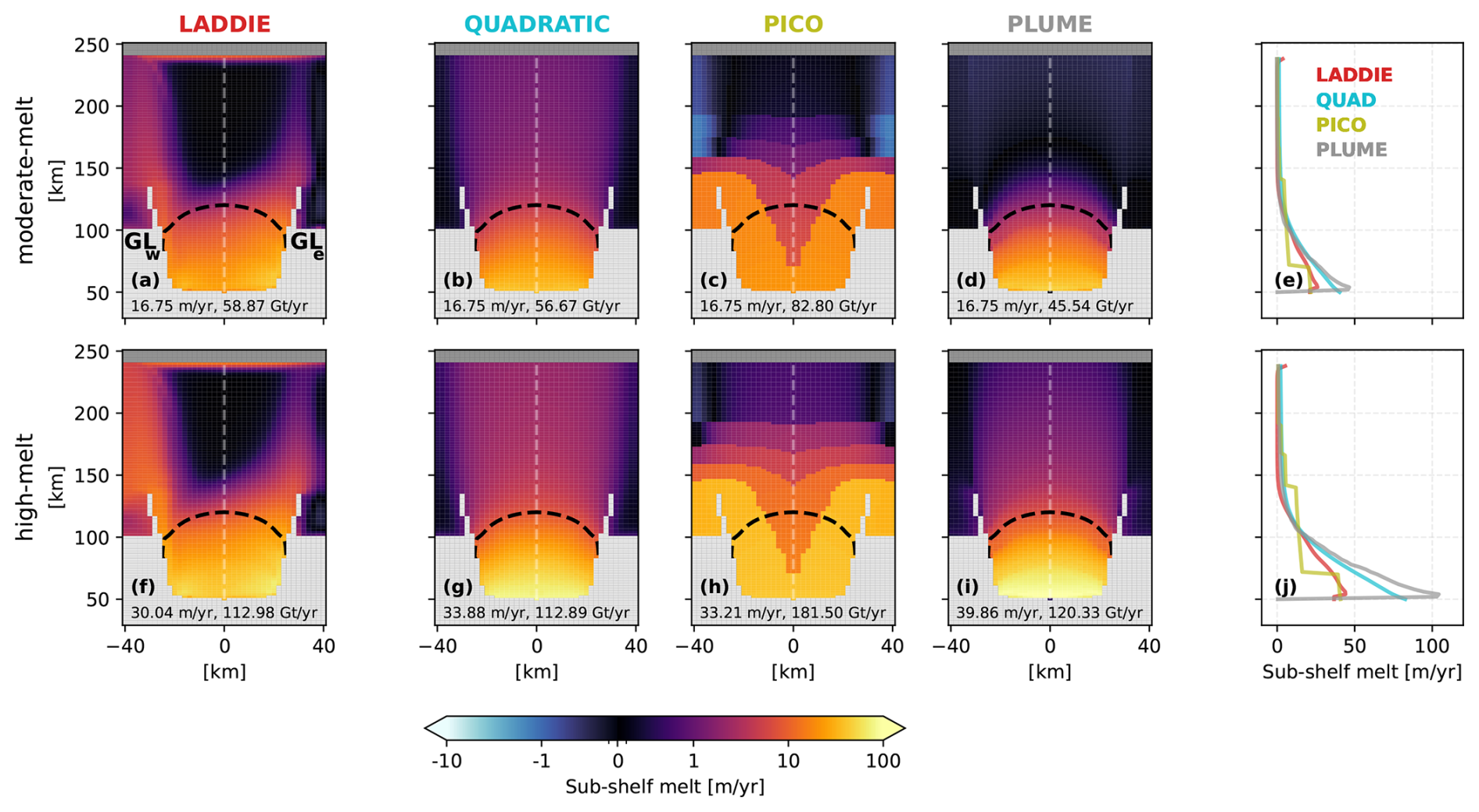
Figure 5Initial melt patterns for the moderate-melt (a–d) and high-melt (f–i) scenario experiments resulting from the tuning procedure (Sect. 2.2.3). The dashed line denotes the 300 m ice shelf draft contour, indicating the deep part of the shelf on which tuning is based. Colours indicate melt rates in m yr−1. The grey area indicates grounded ice, and the blue zone indicates the ocean (so no ice). The averaged deep melt rates (in m yr−1) and integrated melt flux (in Gt yr−1) are given at the bottom of each panel. The right-most panels show melt rates along the central flow line (indicated by grey dashed line in the top-view plots) for the different sub-shelf melt parameterisations in the moderate-melt (e) and high-melt (j) scenarios.
3.2 Comparison with sub-shelf melt parameterisations
3.2.1 Initial melt fields
The initial melt patterns of the parameterised experiments reveal three key differences when compared to the initial melt patterns from the LADDIE experiments (Fig. 5). These differences are largely consistent between the moderate-melt and high-melt scenario and relate to (1) melt rates along the western and eastern flanks of the ice shelf, (2) the distribution of melt near the central grounding line, and (3) the integrated melt flux.
First, melt rates along the western and eastern flanks of the ice shelf differ across the sub-shelf melt implementations, both in the deep tuning zone and in shallower areas. For LADDIE, the Coriolis deflection and topographic steering of the meltwater flow lead to greater melt along the margins than in the centre (Fig. 5a). In contrast, the Quadratic and Plume parameterisations show a much more centralised melt distribution, with minimal melt along the flanks and the east–west-oriented GLw and GLe (Fig. 5b, d). For the Quadratic parameterisation, this is related to these areas being shallow and therefore experiencing low thermal forcing. For the Plume parameterisation, the prescribed flow pathway appears to underestimate the flow convergence towards the shear margins, compared to when the 2D flow is resolved (as in LADDIE). The PICO parameterisation shows enhanced melt rates along the margins (Fig. 5c), similar to LADDIE, but for a different reason. PICO assumes meltwater flow origin along the entire grounding line, whereas in LADDIE, the plume origin is determined by entrainment which is strongest in the deepest regions. This difference causes PICO's melt rates along the margins, beyond the deep tuning area, to exceed those of LADDIE. Additionally, PICO shows enhanced melt at both the GLw and GLe. This contrasts with LADDIE’s pattern, where enhanced melt is only observed at the GLw, where heat transported by the western boundary current can enter the region.
Second, the melt rates along the central flow line reveal a different spatial distribution within the deep tuning area, in particular close to the grounding line (Fig. 5e, j). The Quadratic and Plume parameterisations show substantially higher melt rates close to the grounding line, compared to LADDIE. In contrast, the PICO parameterisation shows melt rates near the grounding line that are more similar to LADDIE’s. However, PICO's box structure results in a much more abrupt decline in melt rates along the central flow line, highlighting its spatially segmented approach, which contrasts with the more gradual reduction observed in LADDIE, Quadratic, and Plume.
Third, the variations in integrated melt flux reflect differences in how melt is distributed between the deeper and shallower regions of the ice shelf, given that average melt rates in the deep tuning area are consistent across all four sub-shelf melt implementations in the moderate-melt scenario. The Quadratic parameterisation shows an integrated melt flux similar in magnitude to LADDIE for both scenarios (Fig. 5b, g), implying a comparable distribution of melt between deep and shallow areas. The PICO parameterisation exhibits a larger integrated flux compared to LADDIE (Fig. 5c). This is due to the high melt rates assigned to the shallow grounding lines along both margins in PICO’s box structure, resulting in more melt occurring in shallower regions. The Plume parameterisation shows the smallest integrated flux (Fig. 5d), with only little melt outside the deep tuning area, indicating lower melt rates in shallow areas relative to LADDIE. Note that in the high-melt scenario the Plume parameterisation produces a larger integrated flux than LADDIE (Fig. 5f, i). This is mainly explained by the increased deep melt rates relative to LADDIE.
Lastly, we remark that the parameterisations exhibit a greater sensitivity to warming, compared to LADDIE. This follows from the averaged deep melt rates for the high-melt scenario for the parameterised melt fields (Fig. 5g, h, i), exceeding the averaged LADDIE deep melt rates (Fig. 5f). The Plume parameterisation has the highest sensitivity, followed by the Quadratic and PICO parameterisations, which have a similar sensitivity.
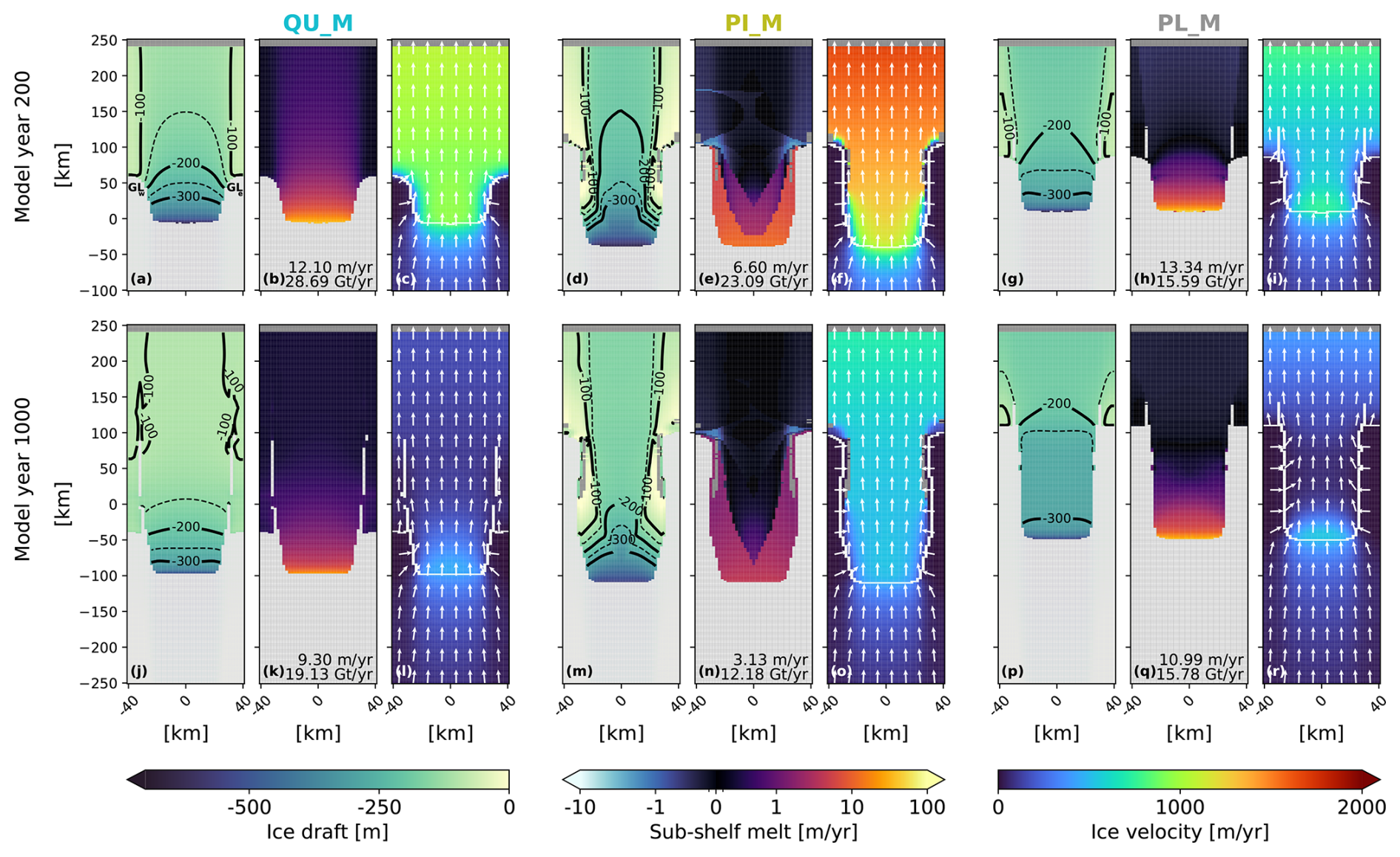
Figure 6Transient response of main variables in the parameterised experiments with moderate forcing (QU_M, PI_M, PL_M). The columns present the ice draft geometry, sub-shelf melt rates, and ice surface velocities. Each row corresponds to a different time slice, indicated to the left of each row. Contours in the first column show ice draft levels, visualised in the same manner as in Fig. 2. The averaged deep melt rates and integrated melt flux are given in the lower-right corner of the sub-shelf melt panels. In the ice surface velocity plots, arrows illustrate the direction of the ice surface velocities, and the white line denotes the grounding line. The east–west-oriented grounding lines at the very edges of the domain are labelled as GLw and GLe in the upper-left panel. Grounded ice is masked in light grey for the ice draft geometry and sub-shelf melt rates. In all panels, the ice-free ocean is masked by dark grey. Dark-grey pixels enclosed by ice shelf pixels indicate areas of melt-through. An animation of this figure, showing time slices every 10 model years, is provided in the Video supplement.
3.2.2 Melt–geometry feedback
In this section, we discuss the feedback between the ice shelf geometry and the sub-shelf melt pattern for the parameterised moderate-melt experiments and compare it to the LA_M experiment (Sect. 3.1). Figure 6 shows the ice shelf draft, sub-shelf melt pattern, and ice surface velocities after 200 and 1000 model years for the QU_M, PI_M, and PL_M experiments. These experiments agree with the LA_M experiment on an initial speed-up of the ice flow and a final stabilisation. The magnitude of ice speed-up and the stabilising mechanisms differ from the LA_M experiment. These differences are related to variations in timing, location, and persistence of enhanced melt, where persistence is defined as the duration over which high melt rates are maintained in a specific region before decreasing again. The following paragraphs provide a more detailed discussion of the feedback between the melt pattern and the geometry for each parameterisation and how it compares with LADDIE. The high-melt scenario results are qualitatively similar (Fig. S2); hence, we only discuss the moderate-melt experiments here.
In agreement with the LA_M experiment, the QU_M experiment shows steepening of the ice draft near the central grounding line over the first 200 model years, indicated by the draft contours moving closer to the central grounding line (Fig. 6a). Unlike for LA_M, this steepening is accompanied with suppressed deep melt rates (Fig. 6b). These suppressed deep melt rates are caused by the onset of melt, which induces ice shelf thinning, resulting in a shallower ice draft which is in contact with colder waters. Additionally, in QU_M, both the GLw and GLe retreat over the first 200 model years (Fig. 6a). This differs from LA_M, where only the GLe retreats due to dynamical detachment along the western shear margin (Fig. 4e). In QU_M, the low melt rates are insufficient to induce a dynamical detachment. Rather, the relatively thick ice maintains a smooth gradient in ice velocity along both margins (Fig. 6c), allowing both margin grounding lines to retreat.
Towards the end of the QU_M experiment, the ice shelf is pinned on the shallow margins, increasing buttressing and reducing ice velocities (Fig. 6j, l). The cause of pinning differs from the cause of readvance in LA_M. For QU_M, pinning at the margins occurs due to thickening, which results from low thermal forcing in these specific areas, caused by the shallow ice draft. In contrast, for LA_M, the thickening at the margins is driven by reduced thermal forcing at the central grounding line, which leads to the migration of the western boundary channel and lower melt rates along the eastern margin. In summary, for QU_M, pinning on the margins is driven by local processes, as this parameterisation neglects meltwater flow, while for LA_M, the readvance is driven by the larger-scale meltwater dynamics.
The PI_M experiment shows high melt rates persisting on both sides after 200 model years (Fig. 6e), in contrast to the LA_M experiment, where melt persists along the western shear margin but weakens along the eastern shear margin. The sustained melt on both sides in the PI_M experiment keeps both margins thin and regionally causes ice shelf melt-through (Fig. 6d). The thin margins allow for dynamical detachment on both sides of the ice shelf (Fig. 6f), similar to that observed at the GLw in the LA_M experiment (Fig. 4h). The dynamical detachment in PI_M has two consequences. First, the GLw and GLe remain at their original position as the ice on the margins is no longer stretched by the downstream ice shelf. Second, it reduces buttressing, allowing for a more rapid ice flow despite the extensively grounded margins.
After 1000 model years, the shear margins remain thin in the PI_M experiment due to persistent margin melt (Fig. 6m, n). This contrasts with LA_M, where shear margin thinning does not persist over this timescale (Fig. 4i, j). Despite the persistent shear margin thinning in PI_M, ice velocities decrease compared to model year 200 (Fig. 6f, o). These reduced velocities are partly due to decreased thermal forcing at the shallower central grounding line, which lowers overall melt rates. Additionally, they are caused by dynamical reattachment near the GLw and GLe, which slightly increases buttressing compared to earlier. However, ice velocities in PI_M remain higher than those observed at the end of the LA_M experiment (Fig. 4l), as the weaker shear margins still allow for a faster ice flow.
The PL_M experiment shows ice draft steepening near the grounding line accompanied by a reduction in averaged deep melt rates over the first 200 model years (Fig. 6g, h), similar to QU_M but contrasting with LA_M. Like LADDIE, the Plume parameterisation relies on ice draft steepness to compute plume velocities. In LADDIE, ice draft steepening establishes a meltwater current along the draft contour line, which enhances melt along this line and further steepens the gradient. This creates a positive feedback between deep melt rates and grounding line steepening. In contrast, the Plume parameterisation generally directs meltwater flow across the draft contour lines (away from the grounding line), preventing the parameterisation from representing this positive feedback. Additionally, while the GLw and GLe have retreated slightly, part of the ice shelf remains pinned on the shallow margins, resulting in lower ice velocities compared to the other experiments (Fig. 6i).
At the end of the PL_M simulation, the GLw and GLe readvance, which suppresses the ice velocities (Fig. 6p, r). The readvance is driven by low thermal forcing at the origin of the plume, located at the shallow GLw and GLe. This low thermal forcing results in limited melt below both flanks of the ice shelf, allowing for regrowth and regrounding (Fig. 6q). The limited melt below the flanks was also observed in the later stages of the LA_M experiment, where it similarly causes readvance of the margins. However, in the Plume parameterisation, the shallow lateral east–west-oriented grounding lines (GLw and GLe) are considered the origin of the plume. As a result, the readvance occurs earlier in the simulation compared to LADDIE, which uses the deeper grounding line as the plume origin.
To synthesise, the Quadratic and Plume parameterisations respond similarly to melt onset. Both capture an initial ice shelf draft steepening, but they fail to represent the positive feedback between enhanced deep melt rates and draft steepening governed by the horizontal meltwater flow adjustment. Over longer timescales, low melt rates along the margins enable stabilisation on these margins through pinning (Quadratic) or a combination of pinning and readvance (Plume). Although this stabilisation resembles that simulated by LADDIE, it arises from different mechanisms tied to the parameterisation's limitations in representing the 2D meltwater flow. For the PICO parameterisation, the melt onset causes thinning and a partial melt-through of the shear margins, reducing buttressing in the short term. This behaviour resembles LADDIE's western margin response but arises from PICO's assumption of meltwater flow origin along the entire grounding line, as opposed to LADDIE's plume originating near the deep grounding line and flowing along the grounding line. Over time, this persistent margin thinning prevents stabilisation, leading to higher ice velocities in PICO compared to LADDIE, where margins thicken due to a weaker meltwater flow.
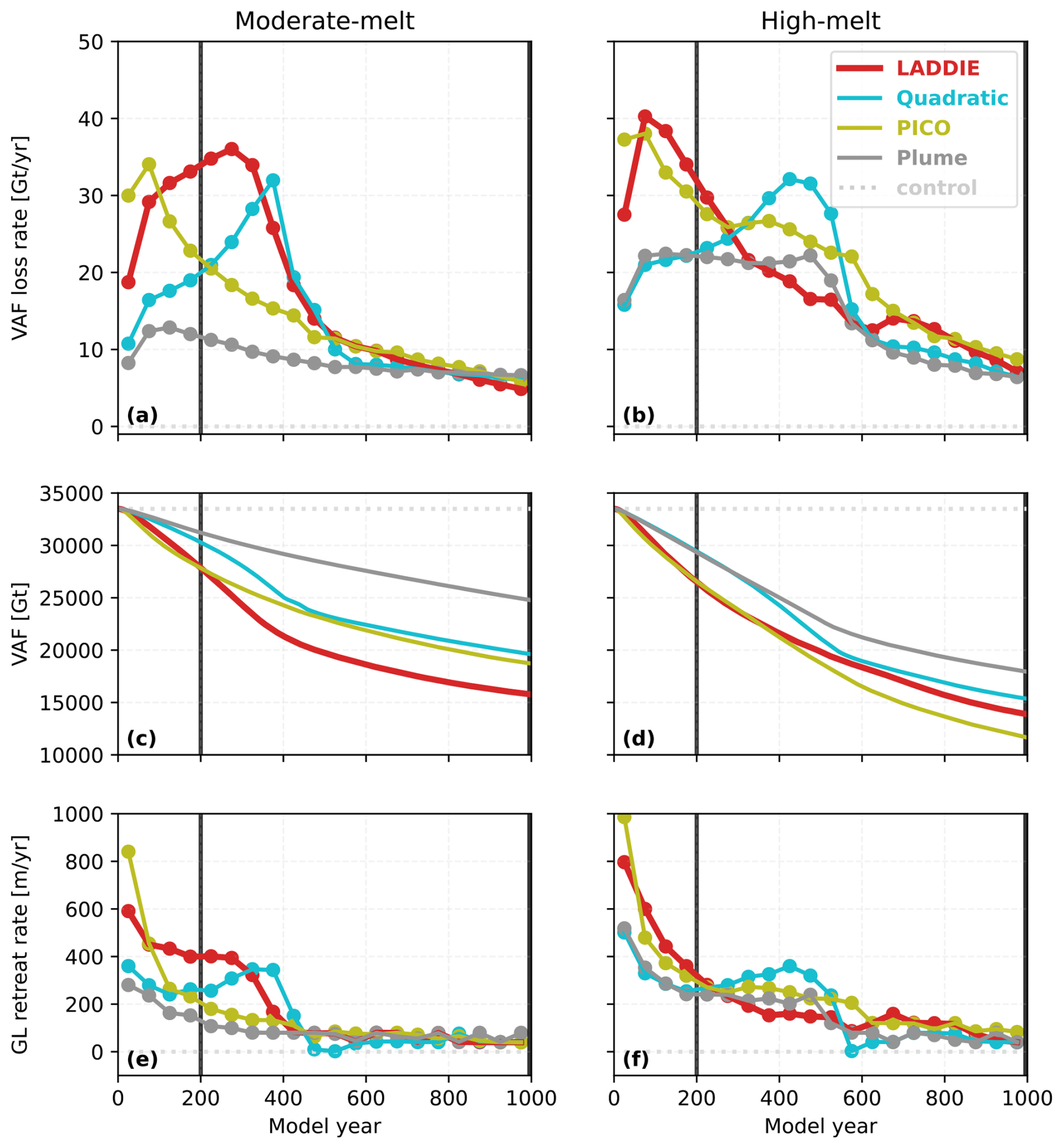
Figure 7Transient response of scalar variables for the entire set of experiments. Volume above flotation (VAF) loss rates (a, b), VAF (c, d), and grounding line retreat rates for the central (Y=0 km) grounding line (e, f) for the moderate-melt (left) and high-melt (right) experiments. VAF loss rates and grounding line retreat rates are calculated as the average rate of change within each consecutive 50-year interval. Thick vertical lines correspond to the time slices presented in Figs. 4 and 6.
3.2.3 Volume above flotation and grounding line retreat
The previous sections covered a qualitative discussion of the melt–geometry feedback for the different moderate-melt simulations. Here, we explore the implications of this feedback on the volume above flotation (VAF) and changes in central grounding line position. By considering these variables, we can quantitatively compare the transient responses of the different simulations and gain deeper insights into their sensitivity to different forcing scenarios. The control experiment, with no melt applied, shows VAF loss rates close to zero throughout the entire simulation, indicating a negligible model drift (Fig. 7a, b).
In all perturbation experiments, the onset of sub-shelf melting potentially triggers marine ice sheet instability (MISI) over the first period of the simulations. Initially, the grounding line is positioned on a retrograde slope, which changes to a prograde slope beyond X=0 km (Fig. 2). Until the grounding line advances across this shift in bed slope, VAF loss and grounding line retreat are driven by a combination of melt-induced thinning and MISI. In most experiments, this crossing occurs within the first 200 years, also being the period which holds the peak rates of VAF loss and grounding line retreat. We note, however, that for a similar geometry, stable grounding line positions can also exist (Gudmundsson et al., 2012). This suggests that MISI may not occur across the entire retrograde bed slope, and in some areas, retreat may be driven only by sub-shelf melting. Once the grounding line crosses the bedrock depression at X=0 km, MISI no longer occurs, and subsequent retreat is governed solely by continued thinning due to melting.
While MISI plays a role in the early retreat phase, the timing and magnitude of peak VAF loss are primarily governed by how LADDIE and the different parameterisations distribute melt beneath the ice shelf. These differences in sub-shelf melt implementation drive the distinct transient responses seen across the moderate- and high-melt scenarios (Fig. 7a, b). In the LADDIE experiments, VAF loss gradually intensifies over the first 100 years, driven by the positive feedback between ice draft steepness and deep melt rates and by thinning along the western boundary. The difference in the duration of strong VAF loss between the moderate-melt and high-melt scenario is explained by the reduced persistence of the western boundary channel in the high-melt scenario due to more frequent ice shelf melt-through (Fig. S1). The Quadratic experiments show a delayed peak VAF loss, relative to the LADDIE experiments. The peak is driven by the retreat of the GLw and GLe, which reduces buttressing and subsequently increases ice velocities later in the simulation. This process of reducing buttressing is slower than the dynamical detachment in the LADDIE experiments, explaining the delay in the peak VAF loss. In contrast, the PICO experiments show an earlier VAF loss peak compared to the LADDIE experiments. This is due to a more rapid margin thinning, inducing earlier dynamical detachment leading to reduced buttressing. The loss rates reduce after about 100 years, when the grounding line retreats past the overdeepening in the bedrock. Past this overdeepening, reduced thermal forcing lowers melt rates, resulting in a gradual decrease in VAF loss rates. Lastly, the Plume experiments show relatively constant VAF loss rates without pronounced peaks. This steady loss is due to persistent pinning along the margins, which restricts ice flow acceleration in the moderate-melt scenario and only moderately allows for it in the high-melt scenario.
Over the first 200 model years, the distinct transient behaviour divides the experiments in two groups, with the LADDIE and PICO experiments showing a stronger VAF loss than the Quadratic and Plume experiments (Fig. 7c, d). This division is also reflected in the grounding line retreat rates over the first 100 model years (Fig. 7e, f). While the initial melt patterns show the highest melt rates near the grounding line for the Plume and Quadratic parameterisation (Fig. 5e, j), the grounding line retreat rates show that these near-grounding line melt rates are not a reliable indicator for the retreat rate. Instead, margin weakening and dynamical detachment allow for a stronger ice speed up in LADDIE and PICO, hence a stronger grounding line retreat. For Quadratic and Plume, strong buttressing prevents a rapid grounding line retreat, regardless of the melt near the grounding line. This suggests that melt along the margins, which is strongly influenced by how the 2D horizontal meltwater flow is represented, may play a more significant role in determining grounding line retreat rates than melt near the grounding line.
On longer timescales, the distinction between the two groups disappears due to a later VAF loss peak of the Quadratic experiments and the different stabilising mechanisms, discussed in Sect. 3.2.2, kicking in. These stabilising mechanisms cause VAF loss rates and grounding line retreat rates to converge to similar magnitudes across the different sub-shelf melt implementations after 600 years. On these timescales, larger-scale ice dynamics appear to be the primary driver of retreat and VAF loss rather than the specific melt pattern, as the latter has little influence due to decreased thermal forcing.
For the resulting VAF at the end of the simulation, however, the choice of sub-shelf melt implementation matters. For the moderate-melt scenario, the melt pattern modelled by LADDIE leads to the largest response in terms of VAF loss over the course of the entire simulation (Fig. 7c). This loss is double that of the Plume experiment and about a quarter more than the losses observed in the Quadratic and PICO experiments. The feedback between steepening and enhanced deep melt rates, accompanied by substantial thinning and local melt-through of the western margin, can sustain a long phase of high VAF loss rates (Fig. 7a). For the Quadratic and PICO experiments, these periods of peak loss are substantially shorter, and for the Plume experiments, VAF loss rates never reach a similar magnitude. For the high-melt scenario, however, the PICO experiment gives the largest amount of VAF loss over the entire simulation (Fig. 7d). This is because the thermal forcing in the high-melt scenario maintains a wider melt-through of the ice shelf margins compared to the moderate-melt scenario. As a result, dynamical detachment occurs over a wider area, leading to elevated VAF loss rates even at the end of the simulation (Fig. S2). In contrast, the LADDIE experiment in the high-melt scenario still shows dynamical reattachment, as reduced thermal forcing weakens the meltwater circulation (Fig. S1). As a result, the final VAF loss in the PICO experiment is over 10 % greater than that in the LADDIE experiment. The Plume experiment shows the least VAF loss; however, the difference with LADDIE is reduced relative to the moderate-melt scenario.
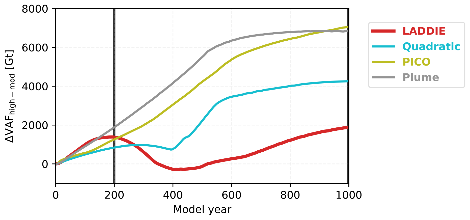
With melt along the margins influencing transient VAF loss and grounding line retreat, we argue it also plays a key role in driving differences in melt sensitivity to the forcing scenario. The additional VAF loss in the high-melt scenario compared to the moderate-melt scenario (ΔVAFhigh-mod) reveals that LADDIE shows a lower sensitivity to the imposed temperature increase compared to the parameterised experiments (Fig. 8). We attribute the low sensitivity in LADDIE to the difference in the persistence of the western boundary channel between the moderate-melt and high-melt scenarios. In the moderate-melt scenario, the channel persists longer, enabling a prolonged phase of dynamical detachment and reduced buttressing. In contrast, in the high-melt scenario, amplified melt in the channel causes localised melt-through, which disrupts the channel (negative feedback), thereby shortening the period of reduced buttressing compared to the moderate-melt scenario (Fig. S1).
For the parameterised experiments, melt along the margins determines the moment of repinning on the lateral margins (Quadratic, Plume) and the extent of ice shelf melt-through (PICO), which influence the VAF, as well as its sensitivity to ocean temperature increase, through their effects on buttressing. For the Quadratic parameterisation, the sensitivity between the scenarios increases sharply after 400 years. This coincides with the moment of pinning in the moderate-melt experiment, where increased buttressing slows down the ice flow. In contrast, the high-melt experiment continues to experience sufficient melt, preventing the ice from repinning just yet. For the PICO parameterisation, thermal forcing at depth at the central grounding line controls melt rates along the margins. Higher temperatures at depth in the high-melt scenario cause widespread melt-through, reducing buttressing and increasing VAF loss compared to the moderate-melt scenario. For the Plume parameterisation, early repinning in the moderate-melt scenario allows the additional VAF loss in the high-melt scenario to accumulate until the high-melt simulation itself also reaches the point of repinning. This again shows that the delay in possible repinning is linked to the stronger VAF loss in a high-melt scenario.
In summary, the timing and magnitude of peak VAF loss vary among the parameterisations and LADDIE, driven by the distribution of melt, particularly along the shear margins. Melt along these margins influences the persistence of the western boundary current in LADDIE, the timing of repinning in Quadratic and Plume, and the extent of melt-through in PICO. As such, it is a key factor that governs the transient VAF loss and grounding line retreat. It also impacts the sensitivity to temperature increases, with the parameterisations showing a greater sensitivity than LADDIE on timescales beyond 300 years. Since the magnitude and persistence of margin melt is influenced by the way the 2D flow is represented, this representation of 2D flow is critical for both the transient behaviour and sensitivity to increased forcing.
Over the first centuries of our LADDIE experiments, the feedback between ice draft steepening and enhanced deep melt rates strengthens the western boundary current, leading to a persistent thinning of the western margin. This margin thinning results in a dynamical detachment between grounded and floating ice on the western side, which leads to reduced buttressing and speed-up of the ice flow, resembling observations of the Crosson ice shelf (MacGregor et al., 2012; Goldberg et al., 2016; Lilien et al., 2018). Furthermore, the western margin thinning aligns with previous modelling studies that identified amplified melt rates on the Coriolis-favoured side of an ice shelf (Goldberg et al., 2012; Gladish et al., 2012). The period of sustained weakening, coinciding with a period of strong volume loss, also supports findings from studies indicating that volume loss is highly sensitive to shear-zone melt (Jordan et al., 2018; Feldmann et al., 2022). Although our simulations are schematic in terms of geometry and forcing, we see qualitatively similar behaviour. Hence, we believe that these observations of Crosson ice shelf can likely be explained by the 2D horizontal meltwater flow.
The phase of strong volume loss is followed by a phase of weaker volume loss as the meltwater circulation weakens and the ice shelf is pinned on the eastern margin, highlighting a distinct transient behaviour. The weakening circulation results from two main factors: first, the reduced heat availability at the central grounding line following its retreat; and second, feedbacks between areas of melt-through and the disruption of the boundary current. With respect to the latter, in LADDIE, the treatment of the open boundary conditions between ice-covered and ice-free cells allows heat and momentum to escape from the cavity, disrupting the downstream meltwater flow. In reality, sea ice may form over these areas, limiting heat loss and potentially allowing the western boundary current to persist. This could prolong the phase of enhanced melt along the full western shear margin, delaying the phase of weaker volume loss. However, observations also indicate that polynyas near basal channels can remain open (Alley et al., 2016). This implies that LADDIE’s representation of heat loss through ice-free areas may still realistically represent key aspects of the system.
LADDIE's ability to capture the margin-specific melt-through and feedbacks between melt and circulation leads to a different response from the sub-shelf melt parameterisations. The parameterisations either lack boundary melt (Quadratic, Plume), preventing melt-through of the western margin, or introduce melt through prescribed melting along the majority of the grounding line, hindering a recovery of the margins later in the simulation (PICO). These limitations in the parameterisations lead to different predictions of potential zones of ice shelf weakening, which might also apply when more realistic geometries are considered. Moreover, the parameterisations fail to replicate the transient behaviour observed in the LADDIE experiments, particularly in the timing and magnitude of peak volume loss. Altogether, this demonstrates that resolving the 2D horizontal meltwater layer dynamics leads to a distinct dynamical ice sheet response not captured by the parameterisations discussed.
Our LADDIE experiments replicate and expand upon key processes hypothesised and demonstrated in earlier studies. For example, Payne et al. (2007) used a model similar to LADDIE on a steady ice shelf draft of Pine Island Glacier and found high melt rates at the grounding line due to a strong ice draft steepness. They hypothesised that the positive feedback between steepening of the ice draft and higher melt rates would finally be compensated by the ice flow, which our simulations indeed confirm. Additionally, Sergienko (2013) showed that melt channel evolution occurs in the absence of variations in external forcing, driven solely by internal interactions between the ocean and the ice shelf. Similarly, in our experiments, we observe basal channel migration under constant external forcing.
The idealised framework of our experiments, both in geometry and forcing, necessitates caution when translating our results to realistic geometries. Our experimental geometry resembles the Pine Island ice shelf in terms of horizontal scale and position within grounded margins. For this ice shelf, melt along the western margin proved crucial in driving volume loss; however, this may not necessarily hold for ice shelves with wider grounding lines and multiple islands, such as the Getz ice shelf. In such cases, melt around these islands, which represents another form of margin melt, is likely to play a more significant role in governing buttressing (Selley et al., 2021). Consequently, differences between LADDIE and the parameterisations in calculating melt rates around such islands may be expected to have a greater impact on the differences in transient volume above flotation. The exact impact of these differences is beyond the scope of this study, as it depends on the specific characteristics of each ice shelf, requiring further investigation.
Using sliding laws other than the Coulomb-limited Schoof sliding law used in our study could yield different surface gradients across the grounding line, which may influence the melt–geometry feedback. For example, sliding laws that do not depend on effective pressure, such as the Weertman power-law relation (Weertman, 1957), may lead to a steeper ice shelf draft near the grounding line. This occurs because they cause a less pronounced reduction in sliding in that region compared to effective pressure-dependent laws like the Schoof sliding law used here. While Schoof sliding already produces a steep draft (see Fig. S3), sensitivity tests suggest that the draft under Weertman sliding could be slightly steeper, albeit marginally (Berends et al., 2023). In LADDIE, a steeper draft could increase meltwater layer velocities at the central grounding line and along the western shear margin. However, the melt–geometry feedback described in Sect. 3.1 is not expected to change fundamentally. Increased meltwater layer velocities may lead to faster thinning of the western shear margin and, consequently, earlier occurrence of melt-through events that disrupt the boundary channel. The latter could shorten the rapid retreat phase via the negative feedback between melt-through events and margin melting discussed in Sect. 3.1. Since earlier sensitivity tests showed only minor differences in draft steepness, switching to a different sliding law is unlikely to substantially affect the melt–geometry feedback for this particular geometry. For the parameterisations, Berends et al. (2023) showed that for this geometry, the choice of sliding has little effect on the final volume compared to the choice of sub-shelf melt parameterisation. However, the choice of sliding law, in combination with more complex geometries, warrants further investigation into the melt–geometry feedback derived from LADDIE and the various parameterisations.
In terms of forcing, the abrupt transition from zero melt at initialisation to the initialised melt fields under the moderate-melt or high-melt scenario introduces a shock to the system. This abrupt change allows us to study the system's response time and resembles the transition from a cold to a warm cavity observed in several modelling studies (Naughten et al., 2021; Jin et al., 2024) or a sudden inflow of warm water due to unpinning (De Rydt et al., 2014) or calving (Bradley et al., 2022). The main caveat of the abrupt switch, compared to gradual temperature changes, is the relatively long timescales of ice dynamics. Ice flow cannot immediately compensate for ice loss driven by sub-shelf melt, allowing high melt rates to dominate the signal in the early years of the simulations. This leads to phenomena such as melt-through of the ice shelf, which occurs when the applied melt rate exceeds the ice shelf thickness divided by the ice sheet model time step (Wearing et al., 2021). Some of these melt-through locations partially recover during the simulations but reopen later, highlighting their intrinsic sensitivity to melt. Altogether, the observations of the western margin melt-through and speed up of the Crosson ice shelf indicate that this simulated process of melt-through may also be induced by relatively moderate changes in ocean temperatures.
Various studies have emphasised the role of calving in influencing ice dynamics (Levermann et al., 2012; Benn and Åström, 2018), prompting us to assess its impact, which we found to be limited. We repeated our experiments, prescribing ice shelf calving in IMAU-ICE when the ice thickness is below 100 m, consistent with the MISOMIP1 protocol (Asay-Davis et al., 2016). While we recognise this as a simplified approach to representing true calving, accurately incorporating it into ice sheet models remains an active area of research (Wilner et al., 2023), so we use the threshold as a first-order approximation. To better understand the influence of calving, we consider its effects through two main mechanisms: (1) changes in melt rate distribution and (2) reductions in ice shelf buttressing. First, calving alters the ice shelf geometry, which in turn can affect the distribution of melt rates. This effect is most evident in the PICO experiments, where calving front retreat modifies the ice-shelf-wide box structure and hence melt pattern (see Video supplement). This restructuring particularly affects melt rates near the deep grounding line, suppressing transient volume loss and grounding line retreat over the initial retreat phase (Fig. S4). In contrast, for LADDIE and the Quadratic and Plume parameterisations, calving front retreat has little influence on melt rates near the grounding line. Second, calving can reduce ice shelf buttressing if it occurs in key areas, such as the shear margins, which play a critical role in buttressing (Fürst et al., 2016). In PICO, although calving along the shear margins may reduce buttressing, its effect is outweighed by the accompanying changes in melt distribution. In the Quadratic and Plume experiments, calving is minimal and confined to the ice shelf front, resulting in a negligible impact on buttressing. In the LADDIE experiments, calving primarily affects ice along the western margin. However, in our default setup, this ice already contributes little to buttressing due to dynamical detachment. As a result, calving, implemented here via a simple thickness threshold, has a limited impact on transient behaviour in LADDIE for this idealised geometry. For more complex geometries or when using more advanced calving laws, further investigation is warranted to better understand the interaction between calving and the melt–geometry feedback for LADDIE and the different parameterisations.
Our results that ice sheet model simulations are sensitive to the representation of sub-shelf melt align with findings from previous studies. We observe a similar magnitude of variation as a result of this modelling choice, consistent with the findings of Berends et al. (2023). Furthermore, we highlight that a more physically advanced representation of sub-shelf melt does not always fall within the uncertainty range of the parameterisations, especially in our moderate-melt experiments. Favier et al. (2019) found that the Plume parameterisation underestimates ice volume loss compared to melt rates computed by a 3D ocean model. Although their implementation of the Plume parameterisation differs from ours, we also find that our Plume experiments underestimate volume loss relative to our LADDIE experiments. Given that tuning targets can affect melt rates in scenarios beyond the tuned case (Burgard et al., 2022), we conducted additional parameterised experiments for the high-melt scenario, adjusting the deep melt rates to match those from the LA_H experiment (Fig. S5). The results demonstrate that our main conclusions remain intact, suggesting that the melt pattern plays a more critical role than the exact magnitude of the melt in determining the transient response. Finally, Lambert and Burgard (2024) showed that a consistent calibration between different sub-shelf melt parameterisations or models does not guarantee consistency in melt sensitivities. We add to this finding that a consistent calibration also does not guarantee a consistent ice sheet response. Overall, our study further underscores that different sub-shelf melt implementations can lead to a divergent ice sheet response over various timescales, regardless of their initial calibration.
We find that the LA_H experiment compares well with 3D cavity-resolving ocean model output for a similar geometry and forcing in the stand-alone ISOMIP+ and coupled MISOMIP1 frameworks (Asay-Davis et al., 2016). In terms of melt rates, the initial ice-shelf average melt rate of approximately 8.2 m yr−1 in LA_H aligns with values between 7.5 and 10.0 m yr−1 reported by Asay-Davis et al. (2016) and Favier et al. (2019). Both studies applied similar external ocean forcing and calibrated their models to achieve deep-cavity melt rates of around 30 m yr−1, consistent with our method. This indicates that LADDIE's partitioning between deep and shallow melt rates is in line with these 3D ocean models. Regarding the circulation patterns, the presence of a western boundary current in LADDIE is in qualitative agreement with the circulation seen across 3D ocean models applied to this geometry. However, melt rates within this current vary across models: some 3D ocean models simulate low melt rates (Vaňková et al., 2025; Zhou and Hattermann, 2020; Scott et al., 2023), while others show high melt rates (Favier et al., 2019; Gwyther et al., 2020). LADDIE’s melt pattern most closely resembles the latter, in particular resembling the pattern produced by NEMO (Favier et al., 2019). In terms of the coupled response, the LA_H experiment shows a 50 % reduction in total melt flux during the first 100 years (see Video supplement), closely matching the MISOMIP1 results presented by Favier et al. (2019). After 100 years, their coupled simulations also exhibit greater volume loss than those using parameterisations, consistent with our findings (Fig. 7b). Furthermore, we observe oscillations in average melt rates, similar to those noted by Zhao et al. (2022), though less pronounced. In our case, the oscillations appear to stem from episodic melt-through events that occasionally disrupt the western boundary current rather than from the exposure of new grid cells.
Although the comparison above demonstrates good agreement between LADDIE and 3D ocean models, we emphasise that our coupled setup is not intended to fully replace the coupling between ice sheet models and 3D cavity-resolving ocean models. Our setup captures changes in ice shelf base geometry leading to different melt patterns and vice versa. However, it does not take into account how changes in meltwater fluxes and geometry impact the general cavity circulation and, consequently, the ambient ocean forcing. De Rydt and Naughten (2024) showed that the evolution of the cavity geometry can substantially alter local ocean dynamics, thereby affecting sub-shelf melt rates. Although computationally demanding, these coupled simulations are crucial for realistic long-term projections. In that context, our setup can be used to employ LADDIE's downscaling functionality by feeding it 3D ocean data to produce physically advanced 2D melt patterns on the ice sheet model grid. This can involve offline-computed 3D ocean simulations or, in the future, online coupling between the ice sheet model and the 3D ocean model, with LADDIE serving as the interface. Besides these downscaling applications, our coupled setup also serves as a stand-alone tool for more process-based studies.
The reality is that many applications of ice sheet models still heavily rely on sub-shelf melt parameterisations (Seroussi et al., 2020, 2024; Hill et al., 2024), which, as our findings reveal, have key limitations compared to a more physically advanced sub-shelf melt representation, especially in how they represent 2D horizontal meltwater flow. These limitations result in different timing and location of ice shelf thinning and melt-through, which are crucial for predicting which parts of the ice shelf are most vulnerable and when an ice shelf region may collapse. As a consequence, they also affect the transient behaviour of volume above flotation, which is essential for obtaining accurate sea level projections. To address these limitations, future research could focus on adapting parameterisations to better capture aspects of 2D horizontal meltwater flow, for instance by allowing meltwater plumes to follow the grounding line rather than following a straight path away from the grounding line (assumed in PICO, Plume). Furthermore, in upcoming model intercomparison projects such as ISMIP7 (Ice Sheet Model Intercomparison Project for CMIP7), it would be valuable to include models that incorporate more physically advanced sub-shelf melt patterns. Given that our LADDIE experiment showed greater volume loss over a millennial timescale under moderate-melt forcing compared to the parameterised experiments, it is important to explore whether the feedback between steepening and enhanced melt along the grounding line and the western margin can also lead to volume loss beyond the parameterised range in more complex geometries with varying forcing.
The coupling of the sub-shelf melt model LADDIE and the ice sheet model IMAU-ICE offers a novel approach to incorporate physically motivated sub-shelf melt patterns in fully dynamical ice sheet simulations. Our simulations conducted with this coupled setup reveal key differences to simulations using widely adopted sub-shelf melt parameterisations in terms of timing, persistence, and the specific location of enhanced melt and eventual melt-through of the ice shelf.
In an idealised geometry, the simulations with LADDIE reveal an important positive feedback mechanism that is not captured by the parameterisations when ocean conditions transition from a cold state with no melt to a warmer state. In both a moderate- and high-warming scenario, the LADDIE experiments reveal an initial steepening of the ice draft near the grounding line, which strengthens the westward meltwater flow along the grounding line, further steepening the ice draft. This, in turn, enhances the western boundary current, leading to increased melt and progressive weakening of the western shear margin of the ice shelf. The commonly used parameterisations assume either no meltwater flow (Quadratic) or meltwater flow directed away from the grounding line (PICO, Plume); hence, they cannot capture this feedback between ice draft steepening and enhanced melt rates along the central and western grounding line.
This enhanced melt along the western shear margin governs the transient behaviour observed in the LADDIE experiments. Initially, thinning of the western margin facilitates a dynamic detachment of the grounded ice from the floating ice, reducing buttressing and accelerating velocities on centennial timescales. On millennial timescales, the meltwater flow weakens due to a reduced thermal forcing near the deep grounding line, suppressing the western boundary channel. This allows the western margin ice shelf to thicken and dynamically reattach to the grounded ice, which ultimately reduces ice velocities and volume loss. Observations of western margin weakening indicate that this process may be important in the recent or future Antarctic response to changes in ocean forcing.
In contrast, the parameterisations cannot replicate this behaviour due to their limited representation of the 2D horizontal meltwater flow. The PICO experiments show high melt rates along the entire grounding line, persisting throughout the full simulation. This forces an initial rapid retreat but prevents later thickening of the margins, thereby reducing buttressing compared to LADDIE. Meanwhile, the Quadratic and Plume experiments reveal low melt at the margins throughout the entire simulation, due to the absence of meltwater flow (Quadratic) or underestimated flow convergence towards the margins (Plume) in these shallow areas. This limited margin melt constrains initial retreat, delaying peak volume loss (Quadratic) or reducing it substantially (Plume).
In summary, our findings suggest that resolving the 2D horizontal meltwater flow introduces new feedbacks and transient behaviour that sub-shelf melt parameterisations, which either neglect or approximate this flow, cannot replicate. The accurate representation of meltwater flow points to an explanation for the weakening of Coriolis-favoured sides of ice shelves and is therefore important to incorporate in more realistic geometries to improve estimates of the future evolution of the Antarctic ice sheet. This can be achieved either by refining existing parameterisations or by directly integrating more detailed melt patterns generated by sub-shelf melt models that resolve the 2D horizontal meltwater flow.
This appendix provides the implementation of the different sub-shelf melt parameterisations in IMAU-ICE.
A1 Quadratic parameterisation
The implementation of the Quadratic parameterisation follows the approach of Favier et al. (2019). Melt rates are computed based on a quadratic relation with the thermal forcing, using
The heat exchange coefficient, γT, is used as tuning parameter; ρw and ρi are the density of ocean water and ice, respectively; cpo is the specific heat capacity of water; and Li is the latent heat of fusion for ice. Values for these parameters are given in Table A1. Ta is the ambient ocean temperature at the depth of the ice shelf base for that particular grid cell. The local freezing temperature, Tf, is defined as a function of salinity, S, and ice shelf base depth, zb, via
Here, λ1, λ2, and λ3 are the liquidus slope, intercept, and pressure coefficient, respectively (Table A1).
Table A1Model parameters used in the sub-shelf melt parameterisations in IMAU-ICE. These parameter settings are also used in LADDIE, except for the PICO-specific EOS parameters.
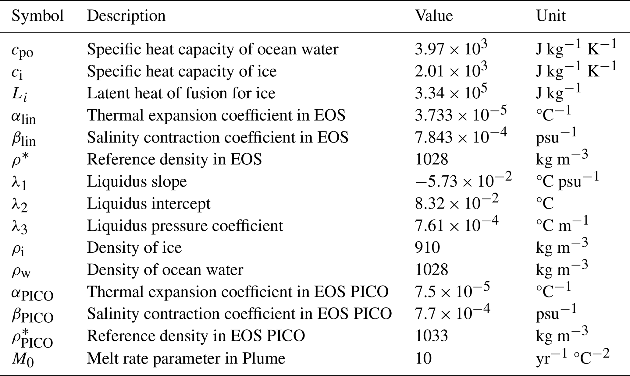
A2 PICO parameterisation
The implementation of PICO follows Reese et al. (2018a). In our experiments, we use the setup with five ocean boxes. Melt rates are computed via
where the subscript k indicates the specific box, with corresponding melt, mk, and ambient temperature and salinity, Ta,k and Sa,k, for that box. γT is treated as a tuning parameter. Moreover, , and , with these parameter values given in Table A1. The ambient ocean conditions Ta,k and Sa,k depend on the overturning flux q, e.g. how much water is transported from one box to the next. pk is the overburden pressure, which introduces a depth dependency within each box. Parameters a, b, and c take the same values as in Reese et al. (2018a). The overturning flux q is defined by
with the overturning coefficient C treated as a tuning parameter. is the reference density in the equation of state (EOS), given in Table A1. Note that we retain the original EOS coefficients from Reese et al. (2018a) for PICO, whereas the forcing, LADDIE, and the Plume parameterisation use values consistent with Asay-Davis et al. (2016). T0 and S0 are the temperature and salinity in box 0, and T1 and S1 are the temperature and salinity in box 1.
A3 Plume parameterisation
The implementation of the Plume parameterisations follows Lazeroms et al. (2018). Melt rates are computed via
Here, M0 is a constant parameter, listed in Table A1; the factor g1(θ) is a function which depends on the basal ice slope θ; Ta is the ambient ocean temperature parameter; Tf,gl is the freezing temperature at the plume origin grounding line; coefficients pk have the same value as reported in Lazeroms et al. (2018); and is defined by
with zb the local ice shelf draft and zgl the ice shelf draft at the grounding line. Length scale l represents the distance from the grounding line at which melting transitions to refreezing and is defined by
It depends on the ambient ocean conditions Ta, freezing temperature at the plume origin Tf,gl, and a slope-dependent factor g2(θ). This slope-dependent factor includes the heat exchange coefficient γT, which we treat as a tuning parameter. For the complete set of equations that describe the Plume parameterisation and its implementation in IMAU-ICE, we refer to Lazeroms et al. (2018). To determine the plume origin, we use an approach similar to the average grounding line origin approach from Lazeroms et al. (2018). Instead of using the 16-direction search algorithm, we average over all grounding line grid cells following Berends et al. (2023).
Table B1 and B2 list the most important model settings for IMAU-ICE and LADDIE, respectively. Additionally, the parameter values shown in Table A1 are also applicable for LADDIE, meaning that both LADDIE and the parameterisations built into IMAU-ICE rely on the same values for these shared parameters. Complete model settings can be found in the configuration files which can be accessed through the link in the data availability statement.
Table B1Main parameter settings for the IMAU-ICE model setup used in this study. Details of the equations and the implementation of these parameters can be found in Berends et al. (2022) and Berends et al. (2023).
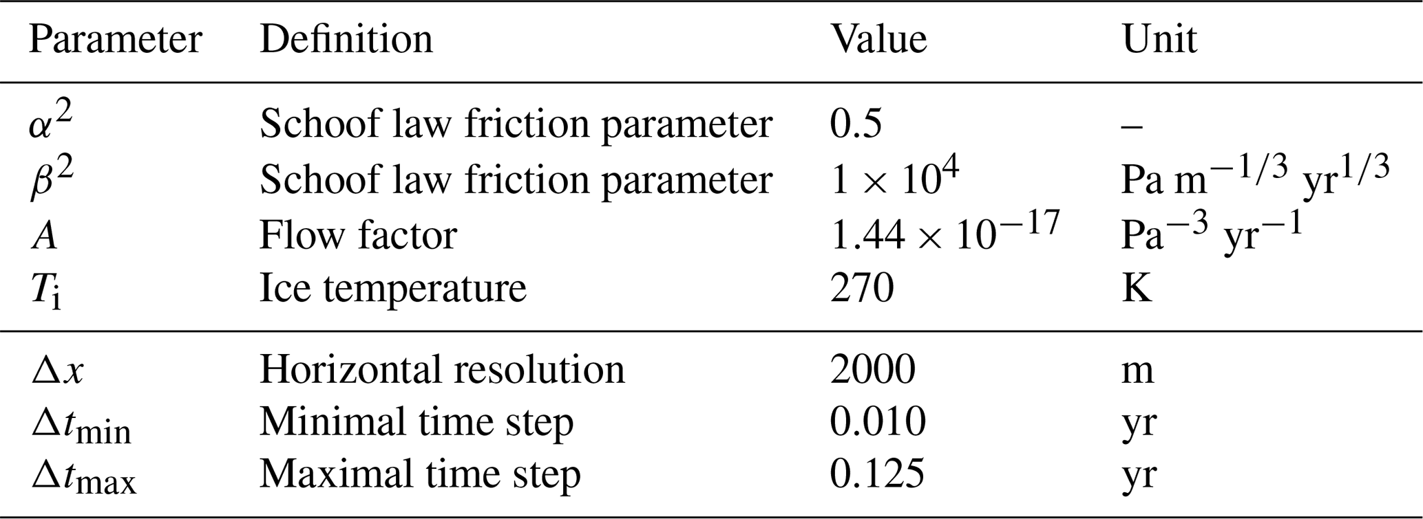
Table B2Main parameter settings for the LADDIE model setup used in this study. Details of the equations and the implementation of these parameters can be found in Lambert et al. (2023).
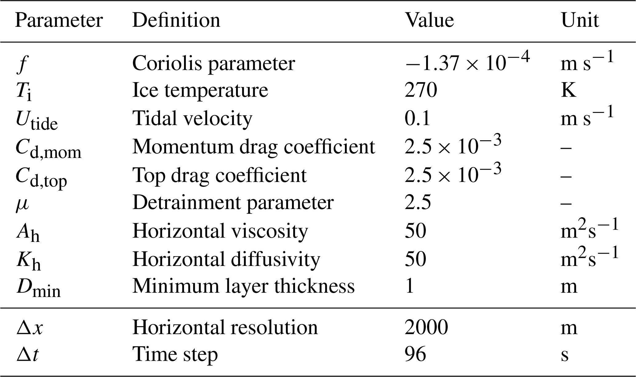
The code for the model versions used in this study, as well as the raw model output and post-processed data, is available via https://doi.org/10.5281/zenodo.14526103 (Jesse, 2024). The scripts to generate the plots are available via https://doi.org/10.5281/zenodo.16881825 (Jesse, 2025).
Animations showing the main variables for all perturbation experiments at a temporal frequency of 10 years are available for download via https://doi.org/10.5281/zenodo.16881825 (Jesse, 2025).
The supplement related to this article is available online at https://doi.org/10.5194/tc-19-3849-2025-supplement.
The conceptualisation was done by FJ, EL, and RSWvdW. FJ conducted the experiments and data analyses; produced the figures; and wrote the manuscript with input from EL and RSWvdW.
The contact author has declared that none of the authors has any competing interests.
Publisher’s note: Copernicus Publications remains neutral with regard to jurisdictional claims made in the text, published maps, institutional affiliations, or any other geographical representation in this paper. While Copernicus Publications makes every effort to include appropriate place names, the final responsibility lies with the authors.
We thank Jan de Rydt, the editor of this paper, for facilitating the review process. Furthermore, we are grateful to the reviewers, Xylar Asay-Davis and Rupert Gladstone, for their thorough assessment and constructive feedback on the manuscript. Franka Jesse used ChatGPT to enhance the readability of specific paragraphs. Following this, the content was reviewed and edited as necessary. Full responsibility is taken for the final publication.
Franka Jesse was funded by Utrecht University. Erwin Lambert was funded by the Netherlands Organisation for Scientific Research (NWO) project HiRISE (grant no. OCENW.GROOT.2019.091).
This paper was edited by Jan De Rydt and reviewed by Xylar Asay-Davis and Rupert Gladstone.
Adusumilli, S., Fricker, H. A., Medley, B., Padman, L., and Siegfried, M. R.: Interannual variations in meltwater input to the Southern Ocean from Antarctic ice shelves, Nat. Geosci., 13, 616–620, https://doi.org/10.1038/s41561-020-0616-z, 2020. a
Alley, K. E., Scambos, T. A., Siegfried, M. R., and Fricker, H. A.: Impacts of warm water on Antarctic ice shelf stability through basal channel formation, Nat. Geosci., 9, 290–293, https://doi.org/10.1038/ngeo2675, 2016. a, b, c
Asay-Davis, X. S., Cornford, S. L., Durand, G., Galton-Fenzi, B. K., Gladstone, R. M., Gudmundsson, G. H., Hattermann, T., Holland, D. M., Holland, D., Holland, P. R., Martin, D. F., Mathiot, P., Pattyn, F., and Seroussi, H.: Experimental design for three interrelated marine ice sheet and ocean model intercomparison projects: MISMIP v. 3 (MISMIP+), ISOMIP v. 2 (ISOMIP+) and MISOMIP v. 1 (MISOMIP1), Geosci. Model Dev., 9, 2471–2497, https://doi.org/10.5194/gmd-9-2471-2016, 2016. a, b, c, d, e, f, g, h
Beckmann, A. and Goosse, H.: A parameterization of ice shelf–ocean interaction for climate models, Ocean Model., 5, 157–170, https://doi.org/10.1016/S1463-5003(02)00019-7, 2003. a
Benn, D. I. and Åström, J. A.: Calving glaciers and ice shelves, Adv. Phys. X, 3, 1513819, https://doi.org/10.1080/23746149.2018.1513819, 2018. a
Berends, C. J., Goelzer, H., Reerink, T. J., Stap, L. B., and van de Wal, R. S. W.: Benchmarking the vertically integrated ice-sheet model IMAU-ICE (version 2.0), Geosci. Model Dev., 15, 5667–5688, https://doi.org/10.5194/gmd-15-5667-2022, 2022. a, b, c
Berends, C. J., Stap, L. B., and Van De Wal, R. S. W.: Strong impact of sub-shelf melt parameterisation on ice-sheet retreat in idealised and realistic Antarctic topography, J. Glaciol., 69, 1434–1448, https://doi.org/10.1017/jog.2023.33, 2023. a, b, c, d, e, f, g
Berger, S., Drews, R., Helm, V., Sun, S., and Pattyn, F.: Detecting high spatial variability of ice shelf basal mass balance, Roi Baudouin Ice Shelf, Antarctica, The Cryosphere, 11, 2675–2690, https://doi.org/10.5194/tc-11-2675-2017, 2017. a
Bradley, A. T., Bett, D. T., Dutrieux, P., De Rydt, J., and Holland, P. R.: The Influence of Pine Island Ice Shelf Calving on Basal Melting, J. Geophys. Res.-Ocean., 127, e2022JC018621, https://doi.org/10.1029/2022JC018621, 2022. a
Bueler, E. and Brown, J.: Shallow shelf approximation as a “sliding law” in a thermomechanically coupled ice sheet model, J. Geophys. Res.-Earth, 114, F03008, https://doi.org/10.1029/2008JF001179, 2009. a
Burgard, C., Jourdain, N. C., Reese, R., Jenkins, A., and Mathiot, P.: An assessment of basal melt parameterisations for Antarctic ice shelves, The Cryosphere, 16, 4931–4975, https://doi.org/10.5194/tc-16-4931-2022, 2022. a, b
Cornford, S. L., Seroussi, H., Asay-Davis, X. S., Gudmundsson, G. H., Arthern, R., Borstad, C., Christmann, J., Dias dos Santos, T., Feldmann, J., Goldberg, D., Hoffman, M. J., Humbert, A., Kleiner, T., Leguy, G., Lipscomb, W. H., Merino, N., Durand, G., Morlighem, M., Pollard, D., Rückamp, M., Williams, C. R., and Yu, H.: Results of the third Marine Ice Sheet Model Intercomparison Project (MISMIP+), The Cryosphere, 14, 2283–2301, https://doi.org/10.5194/tc-14-2283-2020, 2020. a
Davison, B. J., Hogg, A. E., Gourmelen, N., Jakob, L., Wuite, J., Nagler, T., Greene, C. A., Andreasen, J., and Engdahl, M. E.: Annual mass budget of Antarctic ice shelves from 1997 to 2021, Sci. Adv., 9, eadi0186, https://doi.org/10.1126/sciadv.adi0186, 2023. a
De Rydt, J. and Naughten, K.: Geometric amplification and suppression of ice-shelf basal melt in West Antarctica, The Cryosphere, 18, 1863–1888, https://doi.org/10.5194/tc-18-1863-2024, 2024. a, b
De Rydt, J., Holland, P. R., Dutrieux, P., and Jenkins, A.: Geometric and oceanographic controls on melting beneath Pine Island Glacier, J. Geophys. Res.-Ocean., 119, 2420–2438, https://doi.org/10.1002/2013JC009513, 2014. a
Favier, L., Jourdain, N. C., Jenkins, A., Merino, N., Durand, G., Gagliardini, O., Gillet-Chaulet, F., and Mathiot, P.: Assessment of sub-shelf melting parameterisations using the ocean–ice-sheet coupled model NEMO(v3.6)–Elmer/Ice(v8.3), Geosci. Model Dev., 12, 2255–2283, https://doi.org/10.5194/gmd-12-2255-2019, 2019. a, b, c, d, e, f, g, h, i, j
Feldmann, J., Albrecht, T., Khroulev, C., Pattyn, F., and Levermann, A.: Resolution-dependent performance of grounding line motion in a shallow model compared with a full-Stokes model according to the MISMIP3d intercomparison, J. Glaciol., 60, 353–360, https://doi.org/10.3189/2014JoG13J093, 2014. a
Feldmann, J., Reese, R., Winkelmann, R., and Levermann, A.: Shear-margin melting causes stronger transient ice discharge than ice-stream melting in idealized simulations, The Cryosphere, 16, 1927–1940, https://doi.org/10.5194/tc-16-1927-2022, 2022. a
Fox-Kemper, B., Adcroft, A., Böning, C. W., Chassignet, E. P., Curchitser, E., Danabasoglu, G., Eden, C., England, M. H., Gerdes, R., Greatbatch, R. J., Griffies, S. M., Hallberg, R. W., Hanert, E., Heimbach, P., Hewitt, H. T., Hill, C. N., Komuro, Y., Legg, S., Le Sommer, J., Masina, S., Marsland, S. J., Penny, S. G., Qiao, F., Ringler, T. D., Treguier, A. M., Tsujino, H., Uotila, P., and Yeager, S. G.: Challenges and Prospects in Ocean Circulation Models, Front. Mar. Sci., 6, 65, https://doi.org/10.3389/fmars.2019.00065, 2019. a
Fox-Kemper, B., Hewitt, H. T., Xiao, C., Åðalgeirsdöttir, G., Drijfhout, S. S., Edwards, T. L., Golledge, N. R., Hemer, M., Kopp, R. E., Krinner, G., Mix, A., Notz, D., Nowicki, S., Nurhati, I. S., Ruiz, L., Sallée, J.-B., Slangen, A. B. A., and Yu, Y.: Ocean, cryosphere, and sea level change, in: Climate Change 2021: The Physical Science Basis, Contribution of Working Group I to the Sixth Assessment Report of the Intergovernmental Panel on Climate Change, edited by: Masson-Delmotte, V., Zhai, P., Pirani, A., Connors, S. L., Péan, C., Berger, S., Caud, N., Chen, Y., Goldfarb, L., Gomis, M. I., Huang, M., Leitzell, K., Lonnoy, E., Matthews, J. B. R., Maycock, T. K., Waterfield, T., Yelekći, Ã., Yu, R., and Zhou, B., 1211–1362, Cambridge University Press, Cambridge, United Kingdom and New York, NY, USA, https://doi.org/10.1017/9781009157896.001, 2021. a
Fürst, J. J., Durand, G., Gillet-Chaulet, F., Tavard, L., Rankl, M., Braun, M., and Gagliardini, O.: The safety band of Antarctic ice shelves, Nat. Clim. Change, 6, 479–482, https://doi.org/10.1038/nclimate2912, 2016. a
Gaspar, P.: Modeling the Seasonal Cycle of the Upper Ocean, https://journals.ametsoc.org/view/journals/ (last access: 30 August 2024), 1988. a
Gladish, C. V., Holland, D. M., Holland, P. R., and Price, S. F.: Ice-shelf basal channels in a coupled ice/ocean model, J. Glaciol., 58, 1227–1244, https://doi.org/10.3189/2012JoG12J003, 2012. a, b
Goldberg, D. N., Little, C. M., Sergienko, O. V., Gnanadesikan, A., Hallberg, R., and Oppenheimer, M.: Investigation of land ice-ocean interaction with a fully coupled ice-ocean model: 2. Sensitivity to external forcings, J. Geophys. Res.-Earth, 117, F02038, https://doi.org/10.1029/2011JF002247, 2012. a
Goldberg, D. N., Narayanan, S. H. K., Hascoet, L., and Utke, J.: An optimized treatment for algorithmic differentiation of an important glaciological fixed-point problem, Geosci. Model Dev., 9, 1891–1904, https://doi.org/10.5194/gmd-9-1891-2016, 2016. a
Grosfeld, K. and Sandhäger, H.: The evolution of a coupled ice shelf–ocean system under different climate states, Glob. Planet. Change, 42, 107–132, https://doi.org/10.1016/j.gloplacha.2003.11.004, 2004. a
Gudmundsson, G. H.: Ice-shelf buttressing and the stability of marine ice sheets, The Cryosphere, 7, 647–655, https://doi.org/10.5194/tc-7-647-2013, 2013. a
Gudmundsson, G. H., Krug, J., Durand, G., Favier, L., and Gagliardini, O.: The stability of grounding lines on retrograde slopes, The Cryosphere, 6, 1497–1505, https://doi.org/10.5194/tc-6-1497-2012, 2012. a
Gudmundsson, G. H., Paolo, F. S., Adusumilli, S., and Fricker, H. A.: Instantaneous Antarctic ice sheet mass loss driven by thinning ice shelves, Geophys. Res. Lett., 46, 13903–13909, https://doi.org/10.1029/2019GL085027, 2019. a
Gwyther, D. E., Kusahara, K., Asay-Davis, X. S., Dinniman, M. S., and Galton-Fenzi, B. K.: Vertical processes and resolution impact ice shelf basal melting: A multi-model study, Ocean Model., 147, 101569, https://doi.org/10.1016/j.ocemod.2020.101569, 2020. a
Hill, E. A., Gudmundsson, G. H., and Chandler, D. M.: Ocean warming as a trigger for irreversible retreat of the Antarctic ice sheet, Nat. Clim. Change, 14, 1165–1171, https://doi.org/10.1038/s41558-024-02134-8, 2024. a
Hoffman, M. J., Branecky Begeman, C., Asay-Davis, X. S., Comeau, D., Barthel, A., Price, S. F., and Wolfe, J. D.: Ice-shelf freshwater triggers for the Filchner–Ronne Ice Shelf melt tipping point in a global ocean–sea-ice model, The Cryosphere, 18, 2917–2937, https://doi.org/10.5194/tc-18-2917-2024, 2024. a
Holland, D. M. and Jenkins, A.: Modeling Thermodynamic Ice–Ocean Interactions at the Base of an Ice Shelf, J. Phys. Oceanogr., 29, 1787–1800, https://doi.org/10.1175/1520-0485(1999)029<1787:MTIOIA>2.0.CO;2, 1999. a
Holland, P. R.: The Transient Response of Ice Shelf Melting to Ocean Change, J. Phys. Oceanogr., 47, 2101–2114, https://doi.org/10.1175/JPO-D-17-0071.1, 2017. a
Holland, P. R. and Feltham, D. L.: The Effects of Rotation and Ice Shelf Topography on Frazil-Laden Ice Shelf Water Plumes, J. Phys. Oceanogr., 36, 2312–2327, https://doi.org/10.1175/JPO2970.1, 2006. a
Holland, P. R., Jenkins, A., and Holland, D. M.: The Response of Ice Shelf Basal Melting to Variations in Ocean Temperature, J. Clim., 21, 2558–2572, https://doi.org/10.1175/2007JCLI1909.1, 2008. a
Jenkins, A.: A one-dimensional model of ice shelf-ocean interaction, J. Geophys. Res.-Ocean., 96, 20671–20677, https://doi.org/10.1029/91JC01842, 1991. a
Jenkins, A., Nicholls, K. W., and Corr, H. F. J.: Observation and Parameterization of Ablation at the Base of Ronne Ice Shelf, Antarctica, J. Phys. Oceanogr., 40, 2298–2312, https://doi.org/10.1175/2010JPO4317.1, 2010. a
Jenkins, A., Shoosmith, D., Dutrieux, P., Jacobs, S., Kim, T. W., Lee, S. H., Ha, H. K., and Stammerjohn, S.: West Antarctic Ice Sheet retreat in the Amundsen Sea driven by decadal oceanic variability, Nat. Geosci., 11, 733–738, https://doi.org/10.1038/s41561-018-0207-4, 2018. a
Jesse, F.: Data supporting “Sub-shelf melt pattern and ice sheet mass loss governed by meltwater flow below ice shelves” from Jesse et al., Zenodo [data set], https://doi.org/10.5281/zenodo.14526103, 2024. a
Jesse, F.: Data analysis supporting Jesse et al. (2025) (v1.0), Zenodo [code and video], https://doi.org/10.5281/zenodo.16881825, 2025. a, b
Jin, J., Payne, A. J., and Bull, C. Y. S.: Current reversal leads to regime change in Amery Ice Shelf cavity in the twenty-first century, EGUsphere [preprint], https://doi.org/10.5194/egusphere-2024-1287, 2024. a
Jordan, J. R., Holland, P. R., Goldberg, D., Snow, K., Arthern, R., Campin, J.-M., Heimbach, P., and Jenkins, A.: Ocean-Forced Ice-Shelf Thinning in a Synchronously Coupled Ice-Ocean Model, J. Geophys. Res.-Ocean., 123, 864–882, https://doi.org/10.1002/2017JC013251, 2018. a, b, c
Joughin, I., Smith, B. E., and Schoof, C. G.: Regularized Coulomb Friction Laws for Ice Sheet Sliding: Application to Pine Island Glacier, Antarctica, Geophys. Res. Lett., 46, 4764–4771, https://doi.org/10.1029/2019GL082526, 2019. a
Lambert, E. and Burgard, C.: Brief Communication: Sensitivity of Antarctic ice-shelf melting to ocean warming across basal melt models, EGUsphere [preprint], https://doi.org/10.5194/egusphere-2024-2358, 2024. a
Lambert, E., Jüling, A., van de Wal, R. S. W., and Holland, P. R.: Modelling Antarctic ice shelf basal melt patterns using the one-layer Antarctic model for dynamical downscaling of ice–ocean exchanges (LADDIE v1.0), The Cryosphere, 17, 3203–3228, https://doi.org/10.5194/tc-17-3203-2023, 2023. a, b, c, d, e
Lazeroms, W. M. J., Jenkins, A., Gudmundsson, G. H., and Van De Wal, R. S. W.: Modelling present-day basal melt rates for Antarctic ice shelves using a parametrization of buoyant meltwater plumes, The Cryosphere, 12, 49–70, https://doi.org/10.5194/tc-12-49-2018, 2018. a, b, c, d, e, f
Lazeroms, W. M. J., Jenkins, A., Rienstra, S. W., and van de Wal, R. S. W.: An Analytical Derivation of Ice-Shelf Basal Melt Based on the Dynamics of Meltwater Plumes, J. Phys. Oceanogr., 49, 917–939, https://doi.org/10.1175/JPO-D-18-0131.1, 2019. a
Leguy, G. R., Lipscomb, W. H., and Asay-Davis, X. S.: Marine ice sheet experiments with the Community Ice Sheet Model, The Cryosphere, 15, 3229–3253, https://doi.org/10.5194/tc-15-3229-2021, 2021. a, b
Levermann, A., Albrecht, T., Winkelmann, R., Martin, M. A., Haseloff, M., and Joughin, I.: Kinematic first-order calving law implies potential for abrupt ice-shelf retreat, The Cryosphere, 6, 273–286, https://doi.org/10.5194/tc-6-273-2012, 2012. a
Lhermitte, S., Sun, S., Shuman, C., Wouters, B., Pattyn, F., Wuite, J., Berthier, E., and Nagler, T.: Damage accelerates ice shelf instability and mass loss in Amundsen Sea Embayment, P. Natl. Acad. Sci. USA, 117, 24735–24741, https://doi.org/10.1073/pnas.1912890117, 2020. a
Lilien, D. A., Joughin, I., Smith, B., and Shean, D. E.: Changes in flow of Crosson and Dotson ice shelves, West Antarctica, in response to elevated melt, The Cryosphere, 12, 1415–1431, https://doi.org/10.5194/tc-12-1415-2018, 2018. a
Locarnini, M., Mishonov, A., Baranova, O., Boyer, T., Zweng, M., Garcia, H., Reagan, J., Seidov, D., Weathers, K., Paver, C., Smolyar, I., Baranova, O., Boyer, T., Zweng, M., Garcia, H., Reagan, J., Seidov, D., Weathers, K., Paver, C., and Smolyar, I.: World Ocean Atlas 2018, Vol. 1: Temperature, 52 pp., https://archimer.ifremer.fr/doc/00651/76338/ (last access: 22 November 2024), 2018. a
MacGregor, J. A., Catania, G. A., Markowski, M. S., and Andrews, A. G.: Widespread rifting and retreat of ice-shelf margins in the eastern Amundsen Sea Embayment between 1972 and 2011, J. Glaciol., 58, 458–466, https://doi.org/10.3189/2012JoG11J262, 2012. a
Naughten, K. A., De Rydt, J., Rosier, S. H. R., Jenkins, A., Holland, P. R., and Ridley, J. K.: Two-timescale response of a large Antarctic ice shelf to climate change, Nat. Commun., 12, 1991, https://doi.org/10.1038/s41467-021-22259-0, 2021. a, b
Otosaka, I. N., Shepherd, A., Ivins, E. R., Schlegel, N.-J., Amory, C., van den Broeke, M. R., Horwath, M., Joughin, I., King, M. D., Krinner, G., Nowicki, S., Payne, A. J., Rignot, E., Scambos, T., Simon, K. M., Smith, B. E., Sørensen, L. S., Velicogna, I., Whitehouse, P. L., A, G., Agosta, C., Ahlstrøm, A. P., Blazquez, A., Colgan, W., Engdahl, M. E., Fettweis, X., Forsberg, R., Gallée, H., Gardner, A., Gilbert, L., Gourmelen, N., Groh, A., Gunter, B. C., Harig, C., Helm, V., Khan, S. A., Kittel, C., Konrad, H., Langen, P. L., Lecavalier, B. S., Liang, C.-C., Loomis, B. D., McMillan, M., Melini, D., Mernild, S. H., Mottram, R., Mouginot, J., Nilsson, J., Noël, B., Pattle, M. E., Peltier, W. R., Pie, N., Roca, M., Sasgen, I., Save, H. V., Seo, K.-W., Scheuchl, B., Schrama, E. J. O., Schröder, L., Simonsen, S. B., Slater, T., Spada, G., Sutterley, T. C., Vishwakarma, B. D., van Wessem, J. M., Wiese, D., van der Wal, W., and Wouters, B.: Mass balance of the Greenland and Antarctic ice sheets from 1992 to 2020, Earth Syst. Sci. Data, 15, 1597–1616, https://doi.org/10.5194/essd-15-1597-2023, 2023. a
Paolo, F. S., Fricker, H. A., and Padman, L.: Volume loss from Antarctic ice shelves is accelerating, Science, 348, 327–331, https://doi.org/10.1126/science.aaa0940, 2015. a
Payne, A. J., Holland, P. R., Shepherd, A. P., Rutt, I. C., Jenkins, A., and Joughin, I.: Numerical modeling of ocean-ice interactions under Pine Island Bay's ice shelf, J. Geophys. Res.-Ocean., 112, C10019, https://doi.org/10.1029/2006JC003733, 2007. a
Pelle, T., Morlighem, M., and Bondzio, J. H.: Brief communication: PICOP, a new ocean melt parameterization under ice shelves combining PICO and a plume model, The Cryosphere, 13, 1043–1049, https://doi.org/10.5194/tc-13-1043-2019, 2019. a, b
Pritchard, H. D., Ligtenberg, S. R. M., Fricker, H. A., Vaughan, D. G., van den Broeke, M. R., and Padman, L.: Antarctic ice-sheet loss driven by basal melting of ice shelves, Nature, 484, 502–505, https://doi.org/10.1038/nature10968, 2012. a
Reese, R., Albrecht, T., Mengel, M., Asay-Davis, X., and Winkelmann, R.: Antarctic sub-shelf melt rates via PICO, The Cryosphere, 12, 1969–1985, https://doi.org/10.5194/tc-12-1969-2018, 2018a. a, b, c, d, e, f
Reese, R., Gudmundsson, G. H., Levermann, A., and Winkelmann, R.: The far reach of ice-shelf thinning in Antarctica, Nat. Clim. Change, 8, 53–57, https://doi.org/10.1038/s41558-017-0020-x, 2018b. a
Reese, R., Garbe, J., Hill, E. A., Urruty, B., Naughten, K. A., Gagliardini, O., Durand, G., Gillet-Chaulet, F., Gudmundsson, G. H., Chandler, D., Langebroek, P. M., and Winkelmann, R.: The stability of present-day Antarctic grounding lines – Part 2: Onset of irreversible retreat of Amundsen Sea glaciers under current climate on centennial timescales cannot be excluded, The Cryosphere, 17, 3761–3783, https://doi.org/10.5194/tc-17-3761-2023, 2023. a
Rignot, E. and Jacobs, S. S.: Rapid Bottom Melting Widespread near Antarctic Ice Sheet Grounding Lines, Science, 296, 2020–2023, https://doi.org/10.1126/science.1070942, 2002. a
Rignot, E., Mouginot, J., Scheuchl, B., van den Broeke, M., van Wessem, M. J., and Morlighem, M.: Four decades of Antarctic Ice Sheet mass balance from 1979–2017, P. Natl. Acad. Sci. USA, 116, 1095–1103, https://doi.org/10.1073/pnas.1812883116, 2019. a
Schoof, C.: The effect of cavitation on glacier sliding, Proc. Roy. Soc. A, 461, 609–627, https://doi.org/10.1098/rspa.2004.1350, 2005. a
Scott, W. I., Kramer, S. C., Holland, P. R., Nicholls, K. W., Siegert, M. J., and Piggott, M. D.: Towards a fully unstructured ocean model for ice shelf cavity environments: Model development and verification using the Firedrake finite element framework, Ocean Model., 182, 102178, https://doi.org/10.1016/j.ocemod.2023.102178, 2023. a
Selley, H. L., Hogg, A. E., Cornford, S., Dutrieux, P., Shepherd, A., Wuite, J., Floricioiu, D., Kusk, A., Nagler, T., Gilbert, L., Slater, T., and Kim, T.-W.: Widespread increase in dynamic imbalance in the Getz region of Antarctica from 1994 to 2018, Nat. Commun., 12, 1133, https://doi.org/10.1038/s41467-021-21321-1, 2021. a
Sergienko, O. V.: Basal channels on ice shelves: MELT CHANNELS, J. Geophys. Res.-Earth, 118, 1342–1355, https://doi.org/10.1002/jgrf.20105, 2013. a
Seroussi, H., Nakayama, Y., Larour, E., Menemenlis, D., Morlighem, M., Rignot, E., and Khazendar, A.: Continued retreat of Thwaites Glacier, West Antarctica, controlled by bed topography and ocean circulation, Geophys. Res. Lett., 44, 6191–6199, https://doi.org/10.1002/2017GL072910, 2017. a
Seroussi, H., Nowicki, S., Payne, A. J., Goelzer, H., Lipscomb, W. H., Abe-Ouchi, A., Agosta, C., Albrecht, T., Asay-Davis, X., Barthel, A., Calov, R., Cullather, R., Dumas, C., Galton-Fenzi, B. K., Gladstone, R., Golledge, N. R., Gregory, J. M., Greve, R., Hattermann, T., Hoffman, M. J., Humbert, A., Huybrechts, P., Jourdain, N. C., Kleiner, T., Larour, E., Leguy, G. R., Lowry, D. P., Little, C. M., Morlighem, M., Pattyn, F., Pelle, T., Price, S. F., Quiquet, A., Reese, R., Schlegel, N.-J., Shepherd, A., Simon, E., Smith, R. S., Straneo, F., Sun, S., Trusel, L. D., Van Breedam, J., van de Wal, R. S. W., Winkelmann, R., Zhao, C., Zhang, T., and Zwinger, T.: ISMIP6 Antarctica: a multi-model ensemble of the Antarctic ice sheet evolution over the 21st century, The Cryosphere, 14, 3033–3070, https://doi.org/10.5194/tc-14-3033-2020, 2020. a
Seroussi, H., Pelle, T., Lipscomb, W. H., Abe-Ouchi, A., Albrecht, T., Alvarez-Solas, J., Asay-Davis, X., Barre, J.-B., Berends, C. J., Bernales, J., Blasco, J., Caillet, J., Chandler, D. M., Coulon, V., Cullather, R., Dumas, C., Galton-Fenzi, B. K., Garbe, J., Gillet-Chaulet, F., Gladstone, R., Goelzer, H., Golledge, N., Greve, R., Gudmundsson, G. H., Han, H. K., Hillebrand, T. R., Hoffman, M. J., Huybrechts, P., Jourdain, N. C., Klose, A. K., Langebroek, P. M., Leguy, G. R., Lowry, D. P., Mathiot, P., Montoya, M., Morlighem, M., Nowicki, S., Pattyn, F., Payne, A. J., Quiquet, A., Reese, R., Robinson, A., Saraste, L., Simon, E. G., Sun, S., Twarog, J. P., Trusel, L. D., Urruty, B., Van Breedam, J., van de Wal, R. S. W., Wang, Y., Zhao, C., and Zwinger, T.: Evolution of the Antarctic Ice Sheet Over the Next Three Centuries From an ISMIP6 Model Ensemble, Earth's Future, 12, e2024EF004561, https://doi.org/10.1029/2024EF004561, 2024. a, b
Siahaan, A., Smith, R. S., Holland, P. R., Jenkins, A., Gregory, J. M., Lee, V., Mathiot, P., Payne, A. J., Ridley, J. K., and Jones, C. G.: The Antarctic contribution to 21st-century sea-level rise predicted by the UK Earth System Model with an interactive ice sheet, The Cryosphere, 16, 4053–4086, https://doi.org/10.5194/tc-16-4053-2022, 2022. a
Smith, R. S., Mathiot, P., Siahaan, A., Lee, V., Cornford, S. L., Gregory, J. M., Payne, A. J., Jenkins, A., Holland, P. R., Ridley, J. K., and Jones, C. G.: Coupling the U.K. Earth System Model to Dynamic Models of the Greenland and Antarctic Ice Sheets, J. Adv. Model. Earth Sy., 13, e2021MS002520, https://doi.org/10.1029/2021MS002520, 2021. a
Vaňková, I., Asay-Davis, X., Branecky Begeman, C., Comeau, D., Hager, A., Hoffman, M., Price, S. F., and Wolfe, J.: Subglacial discharge effects on basal melting of a rotating, idealized ice shelf, The Cryosphere, 19, 507–523, https://doi.org/10.5194/tc-19-507-2025, 2025. a
Wearing, M. G., Stevens, L. A., Dutrieux, P., and Kingslake, J.: Ice-Shelf Basal Melt Channels Stabilized by Secondary Flow, Geophys. Res. Lett., 48, e2021GL094872, https://doi.org/10.1029/2021GL094872, 2021. a, b
Weertman, J.: On the Sliding of Glaciers, J. Glaciol., 3, 33–38, https://doi.org/10.3189/S0022143000024709, 1957. a
Wilner, J. A., Morlighem, M., and Cheng, G.: Evaluation of four calving laws for Antarctic ice shelves, The Cryosphere, 17, 4889–4901, https://doi.org/10.5194/tc-17-4889-2023, 2023. a
Zhao, C., Gladstone, R., Galton-Fenzi, B. K., Gwyther, D., and Hattermann, T.: Evaluation of an emergent feature of sub-shelf melt oscillations from an idealized coupled ice sheet–ocean model using FISOC (v1.1) – ROMSIceShelf (v1.0) – Elmer/Ice (v9.0), Geosci. Model Dev., 15, 5421–5439, https://doi.org/10.5194/gmd-15-5421-2022, 2022. a
Zhou, Q. and Hattermann, T.: Modeling ice shelf cavities in the unstructured-grid, Finite Volume Community Ocean Model: Implementation and effects of resolving small-scale topography, Ocean Model., 146, 101536, https://doi.org/10.1016/j.ocemod.2019.101536, 2020. a
Zinck, A.-S. P., Wouters, B., Lambert, E., and Lhermitte, S.: Unveiling spatial variability within the Dotson Melt Channel through high-resolution basal melt rates from the Reference Elevation Model of Antarctica, The Cryosphere, 17, 3785–3801, https://doi.org/10.5194/tc-17-3785-2023, 2023. a
- Abstract
- Introduction
- Methods
- Results
- Discussion
- Conclusions
- Appendix A: Details on sub-shelf melt parameterisations
- Appendix B: Model settings
- Code and data availability
- Video supplement
- Author contributions
- Competing interests
- Disclaimer
- Acknowledgements
- Financial support
- Review statement
- References
- Supplement