Retrieving frozen ground surface temperature under the snowpack in the Arctic permafrost area from SMOS observations

We developed and evaluated a new method to retrieve ground surface temperatures T_g below the snowpack from Soil Moisture and Ocean Salinity (SMOS) satellite L-band brightness temperatures (BTs). The study was performed over 21 reference sites providing in situ ground temperatures T_g-insitu in Northern Alaska from 2011 to 2020, representative of Arctic tundra underlined by continuous permafrost, and with various open water fractions. Values of T_g were obtained by inverting two types of microwave emission models (MEMs) tailored for winter Arctic tundra environments. The first MEM assumed homogeneous SMOS pixels and optimized the surface roughness H_r,gs. We observed the important influence of the frozen water bodies on T_g retrievals. Accordingly, we used a second more advanced MEM that accounts for the water surfaces within the SMOS pixels and describes their emission using an optimized water–ice interface roughness parameter, H_r,wi. For sites with water fraction < 0.04, our methods (median R = 0.60) outperformed the European Centre for Medium-Range Weather Forecasts reanalysis (ERA5) product (median R = 0.51) with respect to the reference sites. The bias between retrieved and in situ temperature was slightly negative (median bias = −0.2 °C). For sites with water fraction > 0.20, our water fraction correction reduced the bias, but the correlation of the T_g retrievals remained lower than that of ERA5. This study opens a new avenue for monitoring T_g below the snowpack in the Arctic using L-band BT, by inversion of a relatively simple MEM and limited auxiliary data. Extending this study to the whole Arctic area and taking advantage of the 15 years of SMOS data to study spatio-temporal variability of winter T_g in Arctic environments is extremely promising.

1 Introduction

The ground surface temperature T_g is a key parameter for physical land surface processes. The observed increase in the surface air temperatures over the last decades (Druckenmiller and Jeffries, 2019) and T_g (Biskaborn et al., 2019) in the Arctic regions induced changes in land surface energy and water balance, affecting weather and climate at local and global scales (Schuur et al., 2015; Chadburn et al., 2017; Turetsky et al., 2020). Changes in T_g affect surface runoff and hydrological processes (Rouse et al., 1997; Ala-Aho et al., 2021) and the ecosystem dynamics (Wang et al., 2019). In snow-covered conditions, T_g temporal dynamics are generally decoupled from air temperature (Bartlett et al., 2004; Cao et al., 2020) because of snow thermal insulation capacity (Zhang, 2005; Domine et al., 2019). Hence, T_g modulates the permafrost active layer dynamics and its spatial distribution (Dobiński, 2020). The Arctic freeze/thaw ground state associated with T_g is a key element of Arctic climate change feedbacks as T_g is the main driver of CO₂ release through soil respiration during winter (Natali et al., 2019; Mavrovic et al., 2023). However, meteorological stations over the Arctic are sparse and very few T_g observations are available due to harsh conditions (Shiklomanov, 2012). Model and reanalysis data provide T_g at a global scale covering decades, but in Arctic areas the results remain uncertain (Royer et al., 2021b), mostly during winter when the Arctic is covered by snow (Herrington et al., 2024). Statistical, empirical and machine learning models (Aalto et al., 2018; Lembrechts et al., 2022; Guo et al., 2024) were proposed but the insulation properties of snow coverage remain a major challenge to estimate T_g (Lembrechts et al., 2022).

Satellite remote sensing provides opportunities to map T_g in cold environments (Westermann et al., 2015). The land surface temperature (LST) can be retrieved based on thermal radiometry (e.g., Jiménez-Muñoz et al., 2014). However, during winter, LST corresponds to the temperature of the snow surface (Westermann et al., 2012). High-frequency (f > 10 GHz) passive microwave data (Fily, 2003; Jones et al., 2007; André et al., 2015) showed limited results for determining the T_g under the snowpack (Duan et al., 2020). Moreover, Köhn and Royer (2012) and Mialon et al. (2007) showed that when using Advanced Microwave Scanning Radiometer for EOS (AMSR-E) and Special Sensor Microwave/Imager (SSM/I) observations, the derived LST corresponds to a thin layer (skin) at the air–snow interface. Marchand et al. (2018) showed the potential of using passive microwaves to retrieve T_g by combining AMSR-E and Moderate-Resolution Imaging Spectroradiometer (MODIS) satellite data to inform a land surface scheme. However, the study was performed for a unique site and the integration of remote sensing data in a land surface scheme remains complex and operationally difficult to implement. It is well known that low microwave frequencies (f < 10 GHz) are less sensitive to snow properties, and L-band (protected frequency band f = 1400–1427 GHz, wavelength λ≃ 21 cm) could provide unique information about the frozen ground under the snow (Schwank et al., 2015; Lemmetyinen et al., 2016; Roy et al., 2017).

In this study, we developed a new approach to retrieve T_g under the snowpack in tundra environments from Soil Moisture and Ocean Salinity (SMOS) observations. The emitted radiations observed by SMOS are expressed in terms of brightness temperature (BT), that are predominantly determined by the effective temperature and the emissivity of the observed scene. By considering that the Arctic ground surface remains frozen throughout winter, the ground emissivity remains constant and the BT depends mostly on T_g. However, even if the emissivity (driven by ground permittivity) remains constant, other contributions to the signal, including contributions from snow and water bodies, should be considered in retrieving T_g. We developed a microwave emission model (MEM) for Arctic tundra conditions to address the complex and heterogeneous scene observed at the SMOS footprint scale. The parameterization of central components such as the frozen ground permittivity, the snow layer and the fraction of snow and ice covered water bodies and their effect on T_g retrievals were evaluated. The retrieved T_g were validated against in situ measurements from 21 sites across Northern Alaska and compared with the European Centre for Medium-Range Weather Forecasts (ECMWF) reanalysis (ERA5) ground temperatures T_g-ERA5 (Hersbach, H. et al., 2023). This satellite-based approach opens a new path towards soil temperature monitoring under the snowpack in the Arctic with expected improvement in land and carbon cycle modeling in permafrost area.

2 Datasets

2.1 Brightness temperatures from SMOS

Operated by the European Space Agency (ESA), the SMOS satellite has been acquiring multi-angular BT at L-band since January 2010 (Kerr et al., 2010). We used the SMOS Level 3 brightness temperatures (L3BT) version 330 provided by the Centre Aval de Traitement des Données SMOS (CATDS) (CATDS, 2024). The L3BT are sampled on the global Equal Area Scalable Earth version 2.0 (EASE 2.0 grid, Brodzik et al., 2012) using a cylindrical projection for daily ascending and descending orbits. Both vertical (V) and horizontal (H) polarizations are available for observation (off-nadir) angles θ from 0 to 60° binned over 5° intervals (Al Bitar et al., 2017). The SMOS measurements are affected by radio frequency interferences (RFI) (Daganzo-Eusebio et al., 2013), the consequences of which vary over time, so morning and afternoon orbits were considered separately. The revisit time is shorter than the 3 d revisit at the Equator and enables observations of the study area at least once a day. The BTs are associated with the estimated radiometric accuracy and sample standard deviation obtained in the averaging of measurements into observation angle bins.

2.2 In situ measurements of ground temperatures

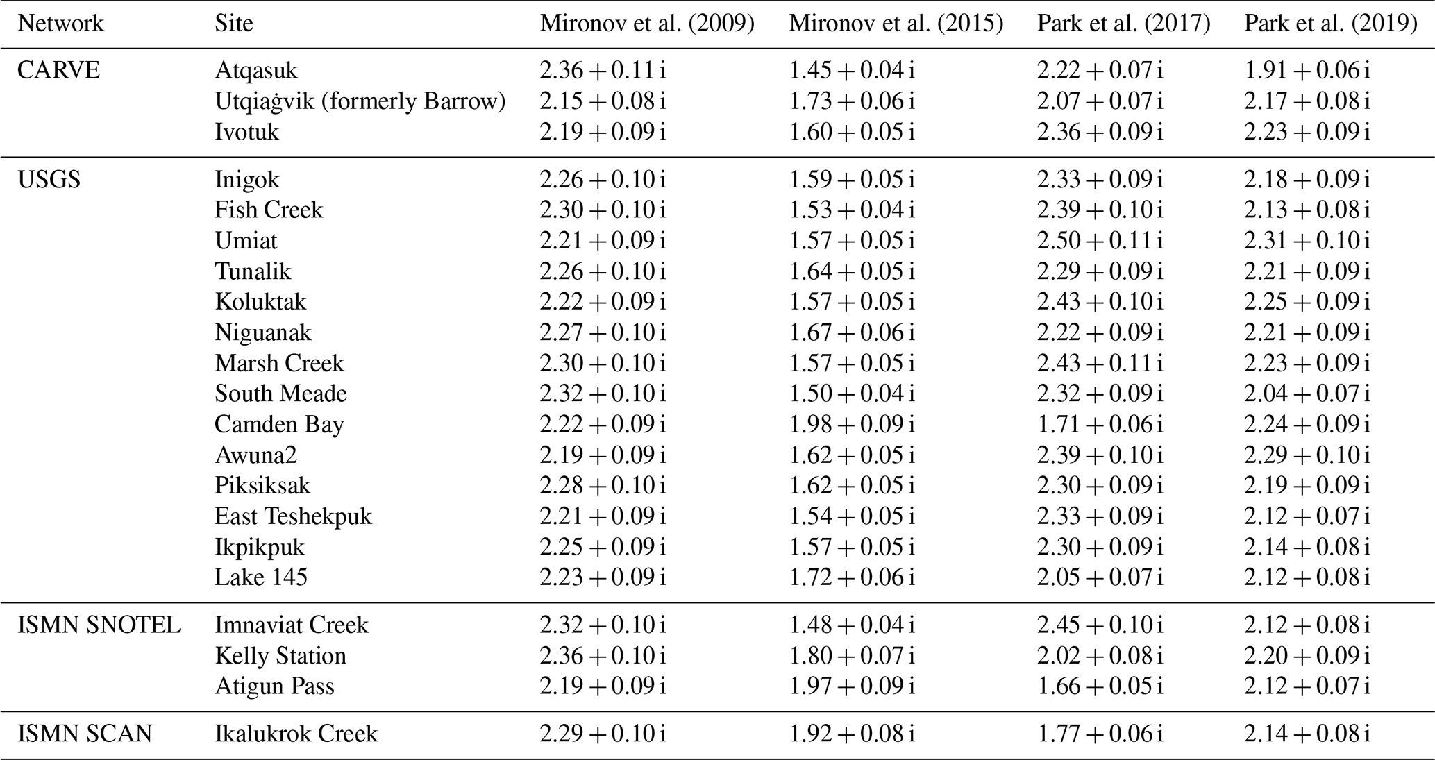
The 21 reference in situ sites are located across Alaska (US), in the Arctic region (Fig. 1 and Table 1). The continuous permafrost landscape integrates numerous lakes, and some sites are located close to the coast (Utqiaġvik (formerly Barrow; Barrow in the figures refers to Utqiaġvik), Lake 145, Fish Creek, Camden Bay), while others are spread inland. All the selected sites are located above the tree line and are representative of the tundra environment with vegetation characterized by low shrubs and mosses (Table 1). SMOS observations are flagged for topography (Mialon et al., 2008), but none of the 21 in situ sites are affected, except for the Atigun pass site which is labeled as moderate topography, i.e., SMOS data quality may be affected by topography. The study sites are part of four different networks. The United States Geological Survey (USGS) (Urban, 2017) provided 14 sites from 1998 to 2019 as part of the Global Terrestrial Network for Permafrost (GTN-P). Three other sites come from the Carbon in Arctic Reservoirs Vulnerability Experiment (CARVE) (Oechel et al., 2016) between 2011 and 2015. The last four sites are part of the Soil Climate Analysis Network (SCAN) (Schaefer et al., 2007) and Snowpack Telemetry (SNOTEL) (Leavesley et al., 2010) and were accessed thanks to the International Soil Moisture Network (ISMN) (Dorigo et al., 2021). The in situ data are available with an hourly temporal resolution and were selected from January 2011 to coincide with SMOS observations. For each site, ground temperatures (T_g-insitu) at variable probing depth are available (Table 1). Other variables such as air temperature at 2 m height and snow depth are available.

Oechel et al. (2016)Urban (2017)Leavesley et al. (2010)Schaefer et al. (2007)

Table 1 In situ stations coordinates with the associated available probe depths. The land cover fractions extracted from the ESA CCI L4 map at 300 m, Version 2.0.7 (2015) (Defourny et al., 2023) using a 40 km diameter buffer around the closest SMOS L3 grid cell center for each study site. Only classes with fractions above 5 % for at least one site are presented.

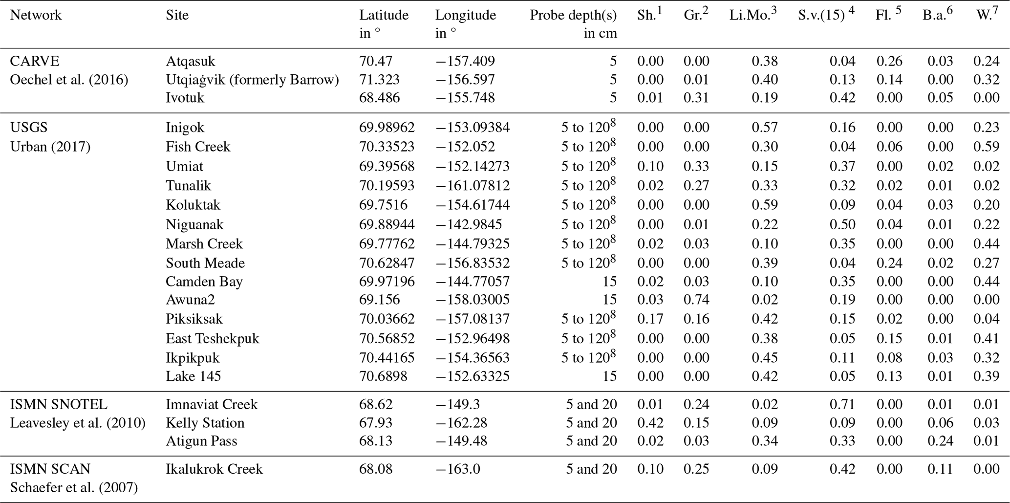
¹ Shrubland, ² Grassland, ³ Lichens and mosses, ⁴ Sparse vegetation (tree shrub herbaceous cover) (< 15 %), ⁵ Shrub or herbaceous cover flooded fresh/saline/brackish water, ⁶ Bare areas, ⁷ Water bodies. ⁸ “5 to 120” refers to all the available depths for the USGS sites, i.e., 5 – 10 – 15 – 20 – 25 – 30 – 45 – 70 – 95 – 120 cm.

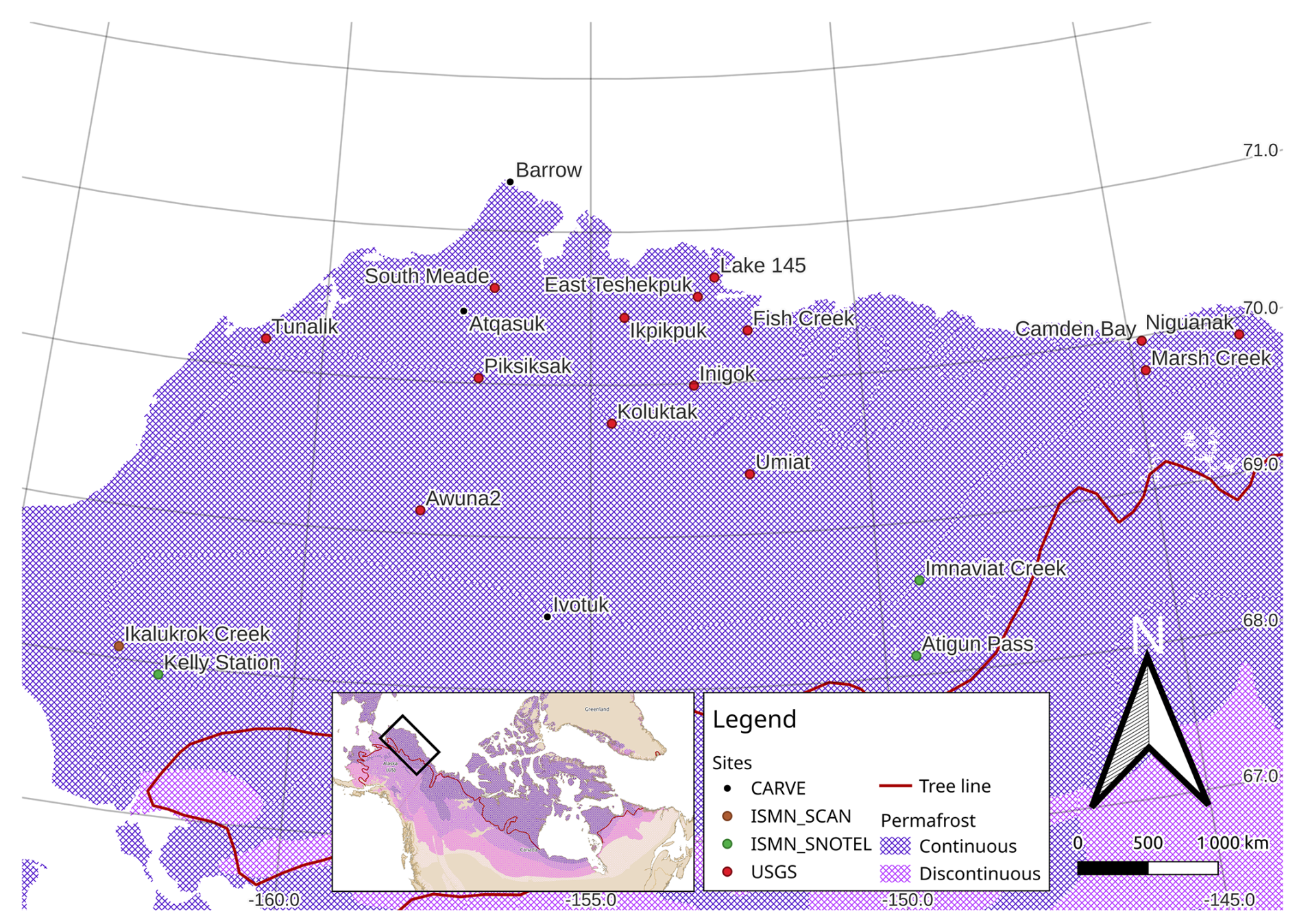
Figure 1 Distribution of the 21 ground-based T_g-insitu stations used as a reference (background: the permafrost extent and tree line from Heginbottom et al. (2002). Sites coordinates are specified in Table 1.

2.3 Model reanalysis ground temperatures

The T_g retrieved from the L3BT was compared to the fifth generation ECMWF reanalysis (ERA5) ground temperature product (Hersbach, H. et al., 2023). We used the shallower soil temperature (Level 1, 0–7 cm depth) T_g-ERA5 provided on a 0.25° resolution grid with an hourly temporal resolution.

2.4 Land cover

The land cover fraction was calculated from the ESA CCI L4 map at a 300 m spatial resolution, Version 2.0.7 (2015) (Defourny et al., 2023). To obtain the fraction of a given land cover class for one grid cell, the number of ESA CCI pixels of the corresponding class was divided by the total number of ESA CCI pixels in a round buffer around the grid cell center. A 40 km diameter buffer zone around each SMOS L3 grid cell center approximately corresponds to a 3 dB antenna pattern cut-off assimilated to the instrumental spatial resolution. The water fraction at each site was within a 40 km buffer. The land cover classes were used for the in situ environment characterization and the analysis of the results. The land cover fractions are summed and listed in Table 1. None of the sites is significantly covered by trees or high vegetation.

3 Methods

3.1 Pre-processing

Our retrievals were based on L-band T_B in H and V polarizations and at angles from 0 to 60°. The T_B were filtered if the RFI ratio (defined as the sum of the RFI flagged instances divided by the sum of the SMOS L1 views combined in each of the L3BT 5° angle bin) was more than 0.1. Due to the RFI situation in North America (Aksoy and Johnson, 2013), observations before 2012 were discarded. In winter, T_g under the snowpack is expected to be diurnally relatively stable (Bartlett et al., 2004). Consequently, we only focused on the daily morning (ascending) orbit passes (approx. 6 am local overpass). We used the T_g-insitu at 5 cm depth to focus on the same ground surface layer for all sites. An exception was made for Awuna2, Camden Bay and Lake 145 where only 15 cm depth measurements were available. For each L3BT, we selected the closest T_g-insitu observed within 30 min of the mean satellite overpass time. The retrieval was performed only when T_g-insitu < −5 °C to ensure that ground conditions satisfy our stable frozen ground permittivity hypothesis (Pardo Lara et al., 2020). We also compared T_g-ERA5 with respect to T_g-insitu. For each site, we considered the nearest neighbor ERA5 node and used the closest time to the satellite overpass time.

3.2 Microwave emission model for the Arctic tundra during winter

Our proposed approach for T_g retrieval required an inversion model based on a MEM (Fig. 2). The upwelling surface $T_{\mathrm{B},\text{surf}}^{\mathrm{p}}\left(\mathit{\theta }\right)$ was considered to be the linear combination of the upwelling BT from the snow-covered ground $T_{\mathrm{B},\mathrm{G}}^{\mathrm{p}}\left(\mathit{\theta }\right)$, from the snow and ice covered water bodies $T_{\mathrm{B},\text{WI}}^{\mathrm{p}}\left(\mathit{\theta }\right)$ weighted by the water bodies fraction ν_wi:

$$\begin{array}{}\text{(1)}& T_{\mathrm{B},\text{surf}}^{\mathrm{p}}\left(\mathit{\theta }\right)=(\mathrm{1}-{\mathit{\nu }}_{\text{wi}})\cdot T_{\mathrm{B},\mathrm{G}}^{\mathrm{p}}\left(\mathit{\theta }\right)+{\mathit{\nu }}_{\text{wi}}\cdot T_{\mathrm{B},\text{WI}}^{\mathrm{p}}\left(\mathit{\theta }\right).\end{array}$$

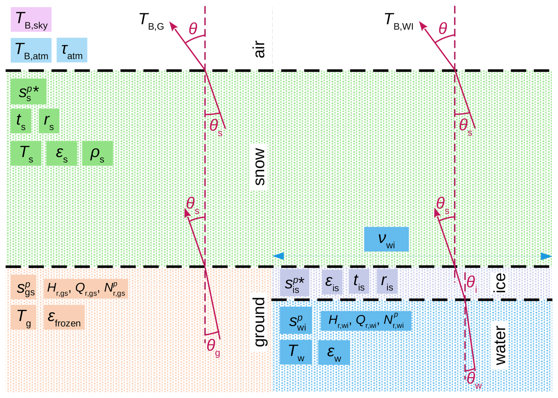
Figure 2 Schematic representation of the MEMs for modeling a winter tundra scene at L-band. MEM_G only considers the left side of the sketch, MEM_G+WI considers both sides.

$T_{\mathrm{B},\mathrm{G}}^{\mathrm{p}}\left(\mathit{\theta }\right)$ and $T_{\mathrm{B},\text{WI}}^{\mathrm{p}}\left(\mathit{\theta }\right)$ were simulated with multi-layer configurations of the Two-Stream model (Schwank et al., 2014) and the Microwave Emission Model of Layered Snowpacks (MEMLS) (Mätzler and Wiesmann, 2012) reflecting the two emission model scenarios depicted in Fig. 2. $T_{\mathrm{B},\mathrm{G}}^{\mathrm{p}}\left(\mathit{\theta }\right)$ resulted from a submodel considering the snow and the atmosphere as two horizontal layers atop the ground which is an infinite half-space. Note that the low vegetation of the tundra is not considered in the submodel. In the case of $T_{\mathrm{B},\text{WI}}^{\mathrm{p}}\left(\mathit{\theta }\right)$, the submodel is made of three horizontal layers (ice, snow and atmosphere) above the water as an infinite half-space. The layers and infinite half-spaces parameterizations are described in the following sections (Sects. 3.2.1–3.2.3); $T_{\mathrm{B},\mathrm{G}}^{\mathrm{p}}\left(\mathit{\theta }\right)$ and $T_{\mathrm{B},\text{WI}}^{\mathrm{p}}\left(\mathit{\theta }\right)$ were also corrected from the atmosphere opacity τ_atm(θ). The deep sky and atmosphere upwelling and downwelling contributions were taken into account as in (Kerr et al., 2020), depending on T_B,sky, T_B,atm(θ) and τ_atm(θ) (Table 2).

Table 2 Input parameters values of the MEM for modeling a winter tundra scene at L-band.

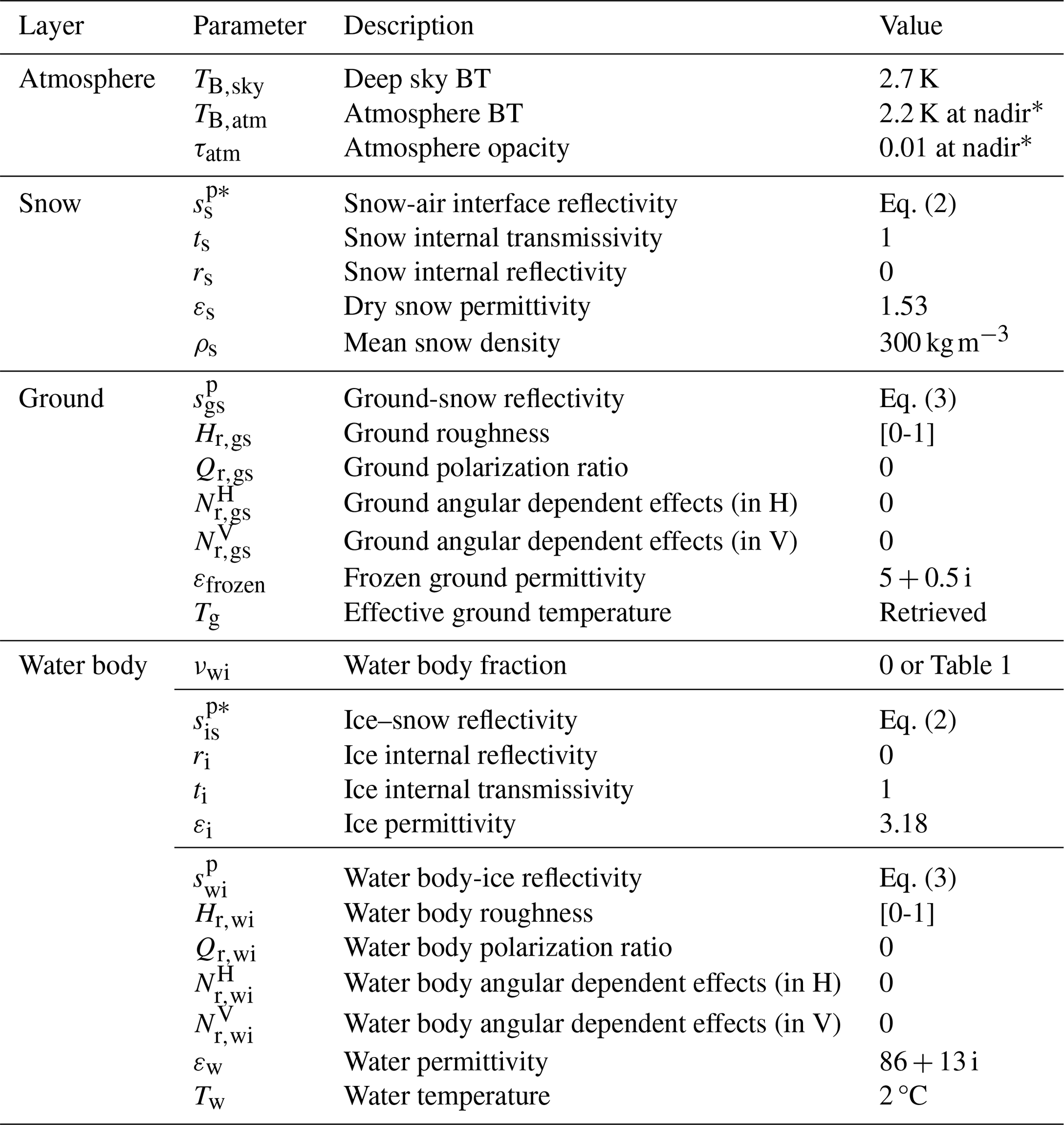
^∗ Example value for θ=0°. For all the angles, T_B,atm and τ_atm are calculated as in Kerr et al. (2020).

Our MEM considered microwave interactions at the interface between two layers: the reflectivity and the refractivity. The reflectivities of the smooth surface between layer n and n+1 are noted as s^H∗(θ) and s^V∗(θ), respectively, and were given by the Fresnel reflection coefficients (Ulaby and Long, 2014):

$$\begin{array}{}\text{(2)}& \begin{array}{rl}& s^{\mathrm{H}\ast }\left(\mathit{\theta }\right)={\left|{\displaystyle \frac{\sqrt{{\mathit{\epsilon }}_n}\cdot A-\sqrt{{\mathit{\epsilon }}_{n+\mathrm{1}}}\cdot B}{\sqrt{{\mathit{\epsilon }}_n}\cdot A+\sqrt{{\mathit{\epsilon }}_{n+\mathrm{1}}}\cdot B}}\right|}^{\mathrm{2}},\\ & s^{\mathrm{V}\ast }\left(\mathit{\theta }\right)={\left|{\displaystyle \frac{\sqrt{{\mathit{\epsilon }}_{n+\mathrm{1}}}\cdot A-\sqrt{{\mathit{\epsilon }}_n}\cdot B}{\sqrt{{\mathit{\epsilon }}_{n+\mathrm{1}}}\cdot A+\sqrt{{\mathit{\epsilon }}_n}\cdot B}}\right|}^{\mathrm{2}},\end{array}\end{array}$$

with A=cos(θ_n) and $B=\sqrt{\mathrm{1}-(\mathrm{1}-A^{\mathrm{2}})\cdot \frac{{\mathit{\epsilon }}_n}{{\mathit{\epsilon }}_{n+\mathrm{1}}}}$, where H and V stand for horizontal and vertical polarization, respectively, θ is the incidence angle and ε_n is the layer n complex dielectric constant.

The H–Q–N model (Wang and Choudhury, 1981) was proposed to empirically consider surface effects (including roughness) in the reflectivity and can be expressed as:

$$\begin{array}{}\text{(3)}& \begin{array}{rl}{s}^{\mathrm{p}}\left(\mathit{\theta }\right)=& \left[(\mathrm{1}-Q_{\mathrm{r}})s_n^{p\ast }\left(\mathit{\theta }\right)+Q_{\mathrm{r}}{s}^{q\ast }\left(\mathit{\theta }\right)\right]\\ & \times \text{exp}\left(-H_{\mathrm{r}}{\text{cos}}^{N_{\mathrm{r}}^{\mathrm{p}}}\left(\mathit{\theta }\right)\right),\end{array}\end{array}$$

where p and q are the two polarizations (q is H (resp. V) when p is V (resp. H)). The surface effects were taken into account with four parameters: the polarization mixing ratio Q_r, the angular effect parameters $N_{\mathrm{r}}^{\mathrm{H}}$, $N_{\mathrm{r}}^{\mathrm{V}}$ and the effective roughness parameter H_r. These four parameters account for not only the geometric roughness effects but also the spatial heterogeneity of the surface characteristics. For instance, Escorihuela et al. (2007) showed H_r dependence on soil moisture content for a ground–air interface. Our values for those parameters are detailed in the following sections and listed in Table 2.

The angle deviation due to refractivity at the interface between the layers n and n+1 is given by Snell–Descartes law:

$$\begin{array}{}\text{(4)}& {\mathit{\theta }}_n=\text{arcsin}\left(\sqrt{{\displaystyle \frac{{\mathit{\epsilon }}_{n+\mathrm{1}}}{{\mathit{\epsilon }}_n}}}\text{sin}{\mathit{\theta }}_{n+\mathrm{1}}\right),\end{array}$$

where ε_n is the layer n complex dielectric constant Ulaby et al. (1984).

3.2.1 Frozen ground parametrization

The bottom-most infinite half-space representing the ground was described using the following parameters: T_g, ε_frozen, H_r,gs, Q_r,gs, $N_{\mathrm{r},\text{gs}}^{\mathrm{p}}$ (see Fig. 2). The ground-snow interface reflectivity $s_{\text{gs}}^{\mathrm{p}}$ was obtained from Eqs. (2) and (3). This study aimed to retrieve the ground surface temperature T_g by considering a fixed and constant ground permittivity in frozen conditions. Various models describe the ground permittivity at 1.4 GHz (Mironov et al., 2009; Bircher et al., 2016; Park et al., 2017), but very few in the case of frozen ground (Hallikainen et al., 1985; Mironov et al., 2015). The permittivity of a frozen ground was set to ε_frozen = 5.0 + 0.5 i, similar to past studies (Schwank et al., 2014; Holmberg et al., 2024) and SMOS algorithm (Kerr et al., 2020). We considered the ground surface reflectivity as in Eq. (3) accounting for various effects including roughness using four parameters (H_r,gs, Q_r,gs, $N_{\mathrm{r},\text{gs}}^{\mathrm{H}}$ and $N_{\mathrm{r},\text{gs}}^{\mathrm{V}}$). The polarization mixing ratio Q_r,gs (Wang and Choudhury, 1981) as well as the angular effects parameters $N_{\mathrm{r},\text{gs}}^{\mathrm{H}}$ and $N_{\mathrm{r},\text{gs}}^{\mathrm{V}}$) were set to zero, as suggested by several studies (Kerr et al., 2020; Wigneron et al., 2011; Lawrence et al., 2013). The value of H_r,gs was optimized for all the sites using a range of 0 to 1 with 0.1 increments.

3.2.2 Dry snow parametrization

The layer accounting for the snow was defined by its effective temperature T_s, permittivity ε_s, layer internal transmissivity t_s and reflectivity r_s (Fig. 2). According to Schwank et al. (2015) and Rautiainen et al. (2016), dry snow is considered transparent at L-band, i.e., its internal transmissivity and reflectivity are t_s=1 (no absorption) and r_s=0 (no volume scattering), respectively. Consequently, our model became independent of T_s. However, Schwank et al. (2015) showed that air–snow interface impacts on impedance matching can not be ignored, i.e., the snow surface reflectivity $s_{\mathrm{s}}^{\mathrm{p}\ast }\ne \mathrm{0}$. We considered refraction (Eq. 4) and reflection for a smooth air–snow interface (Eq. 2). The dry snow permittivity was set to ε_s=1.53 according to Eq. (4) of Schwank et al. (2015) for a mean snow density ρ_s = 300 kg m³, which corresponds to the high Arctic snowpack average density observed by Derksen et al. (2014) and Roy et al. (2017). We assume a snowpack with the same parameters above the ground and the ice-covered water bodies.

3.2.3 Snow and ice covered water bodies parametrization

During winter, water bodies are fully covered by an ice layer with liquid water remaining below the ice layer (Adams and Lasenby, 1985; Jeffries et al., 2013). The ice layer was defined by its permittivity ε_i = 3.18 (Mätzler, 2006) and considered transparent (internal transmissivity t_i=1 and internal reflectivity r_i=0). However, smooth surface refraction (Eq. 4) and reflection $s_{\text{is}}^{\mathrm{p}\ast }$ (Eq. 2) were taken into account at the ice–snow interface. Similarly to the ground layer, the liquid water layer was defined with T_w, ε_w, H_r,wi, Q_r,wi and $N_{\mathrm{r},\text{wi}}^{\mathrm{p}}$ (Fig. 2). The water temperature T_w was considered constant throughout winter and equal to 2 °C (Oveisy et al., 2012). We consider fresh water whose L-band permittivity ε_w was fixed to 86 + 13 i (Liebe et al., 1991; Mätzler, 2006; Ulaby and Long, 2014). The water–ice interface reflectivity $s_{\text{wi}}^{\mathrm{p}}$ was obtained from Eq. (3), accounting for the water–ice interface heterogeneity: Q_r,wi, $N_{\mathrm{r},\text{wi}}^{\mathrm{H}}$ and $N_{\mathrm{r},\text{wi}}^{\mathrm{V}}$ were set to 0 (Choudhury et al., 1979); the value of H_r,wi was optimized for all the sites in a range of 0 to 2 with an iteration step of 0.1. The water body ν_wi accounted for the area percentage of the considered SMOS node covered by water bodies based on the water class from ESA CCI land cover (Table 1).

3.2.4 Microwave emission model configurations

Figure 2 depicts a schematic of the MEMs and Table 2 lists a summary of the input parameters. This study tested two configurations: one considering a homogeneous scene with only ground (hereafter named MEM_G) and one with a heterogeneous scene composed of ground and snow and ice covered water bodies (hereafter named MEM_G+WI).

3.3 Cost function for frozen ground temperature retrievals

Both MEM_G and MEM_G+WI described in Sect. 3.2 were inverted to retrieve the frozen ground temperature T_g, by minimizing the following cost function:

$$\begin{array}{}\text{(5)}& \text{CF}\left(T_{\mathrm{g}}\right)=\sum _{\mathrm{p},{\mathit{\theta }}_k}{\left({\displaystyle \frac{T_{\mathrm{B},\text{obs}}^{\mathrm{p}}\left({\mathit{\theta }}_k\right)-T_{\mathrm{B},\text{sim}}^{\mathrm{p}}({\mathit{\theta }}_k,T_{\mathrm{g}})}{\mathit{\sigma }{T}_{\mathrm{B}}^{\mathrm{p}}\left({\mathit{\theta }}_k\right)}}\right)}^{\mathrm{2}},\end{array}$$

where $T_{\mathrm{B},\text{obs}}^{\mathrm{p}}\left({\mathit{\theta }}_k\right)$ and $T_{\mathrm{B},\text{sim}}^{\mathrm{p}}({\mathit{\theta }}_k,T_{\mathrm{g}})$ are, respectively, the observed and simulated BT for both H and V polarizations and at various incidence angle bins θ_k. The BT standard deviation $\mathit{\sigma }{T}_{\mathrm{B}}^{\mathrm{p}}\left({\mathit{\theta }}_k\right)$ is computed from the estimated radiometric accuracy and sample standard deviation obtained in the averaging of measurements into observation angle bin k.

3.4 Post-processing

The first aim of the post-processing was to reduce the influence of outliers. The retrieved T_g below the first 1 % quantile and above the last 99 % quantile of each site were considered outliers and discarded. We removed the T_g-ERA5 at these dates in the ERA5 time series to ensure that we compared a data pull with the same size. A low short-term variability is expected between T_g under the snowpack that acts like a thermal insulator. The final step smoothed the T_g time series to reduce the impact of the noise in SMOS BT to the retrievals. We used a z-score smoothing, to limit the variations of T_g to 1 standard deviation for a 5 d window. At a date t, the local average $\stackrel{\mathrm{‾}}{T_{\mathrm{g}}^{\mathrm{t}}}$ and standard deviation $\mathit{\sigma }\left(T_{\mathrm{g}}^{\mathrm{t}}\right)$ are calculated for a 5 d window around each $T_{\mathrm{g}}^{\mathrm{t}}$. If $T_{\mathrm{g}}^{\mathrm{t}}>\stackrel{\mathrm{‾}}{T_{\mathrm{g}}^{\mathrm{t}}}+\mathrm{1}\cdot \mathit{\sigma }\left(T_{\mathrm{g}}^{\mathrm{t}}\right)$, $T_{\mathrm{g}}^{\mathrm{t}}$ is replaced by $\stackrel{\mathrm{‾}}{T_{\mathrm{g}}^{\mathrm{t}}}$.

3.5 Metrics

Three statistical indicators were used to assess the comparison between the retrieved T_g and the reference temperatures T_g-insitu ((Entekhabi et al., 2010; Gruber et al., 2020)). The unbiased root-mean-square deviation (ubRMSD) is used for uncertainty estimation as it is corrected from the bias between the two time series (Kerr et al., 2016a; Benninga et al., 2020). The bias corresponds to the mean difference between the compared time series of T_g and T_g-insitu. The Pearson correlation coefficient (R) accounts for the similarities in temporal dynamics of the two time series. Each metric was computed for the whole time series for each site and was provided with its confidence intervals (CI) at 5 % and 95 %. Analytical solutions enabled us to find the CI of the bias, the ubRMSD and R (Gruber et al., 2020). We also evaluated T_g-ERA5 with respect to T_g-insitu with similar metrics.

4 Results

The metrics (bias, R and ubRMSD) for all sites obtained with both MEM_G and MEM_G+WI are summarized in Appendix D. This results section first focuses on the H_r,gs and H_r,wi optimization based on the biases (Sect. 4.1) and then evaluates the T_g retrievals (Sect. 4.2).

4.1 Parameters optimization evaluation

4.1.1 H_r,gs optimization

In the MEM_G configuration, we retrieved T_g by testing H_r,gs values from 0 to 1 with 0.1 increments. Figure 3 shows the biases obtained with all tested H_r,gs and biases obtained with T_g-ERA5 for each site, with respect to T_g-insitu. For all sites, the bias changed in the negative direction with increasing H_r,gs. For sites with ν_wi≤0.04, the biases went from positive down to negative values with increasing H_r,gs, except for Awuna2 and Umiat whose biases remained positive. For sites with ν_wi≥0.20, the biases of numerous sites remained negative and went down close to −30 °C. This suggests that the water bodies strongly affect the T_g retrieval bias. That is why we optimized the value of H_r,gs only on sites less affected by water bodies. For sites with ν_wi≤0.04, the bias was minimized with H_r,gs = 0.8 (average = 0.2 °C, median = −0.2 °C, Q1 = −1.6 °C, Q3 = 0.8 °C, range = 2.4 °C). Surprisingly, the sites with the highest ν_wi (between 0.44 and 0.59) showed positive biases for some H_r,g.

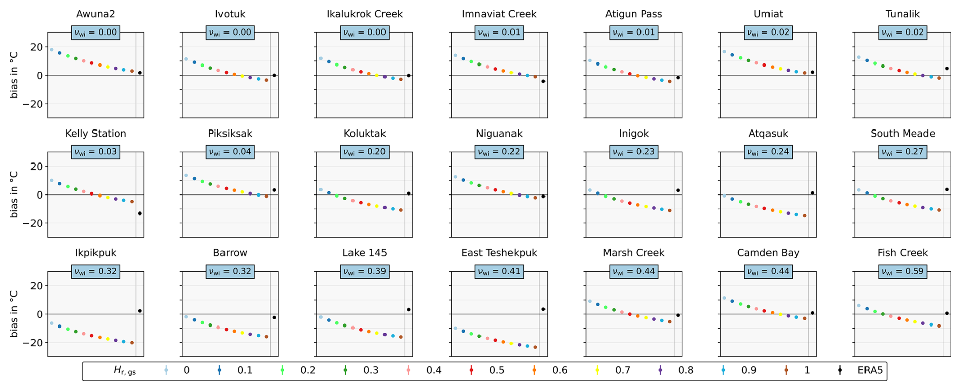
Figure 3 Bias per site for each H_r,gs used in the inversion with the MEM_G model. Each graph corresponds to one site. H_r,gs values are represented by a unique color and are ranged from 0 to 1 on the x axis. The last point of each graph, in black, is obtained with T_g-ERA5. The y axis corresponds to the bias T_g−T_g-insitu. Each point is symbolized with error bars that correspond to the confidence interval. The sites are ordered in ascending order of water fraction (ν_wi in the light blue box).

4.1.2 H_r,wi optimization

The results in Sect. 4.1.1 showed that the T_g retrieval bias strongly depends on water fraction. The MEM_G+WI model accounted for the presence of frozen water bodies (i.e., ν_wi≠0) in the T_B calculation (Fig. 2). In this configuration, T_g was retrieved with different tested H_r,wi values from 0 to 1 with 0.1 increments; H_r,gs was set to 0.8 as shown in Sect. 4.1.1. For each site, Fig. 4 shows the biases obtained with various H_r,wi and compared with T_g-ERA5 bias with respect to T_g-insitu. The higher H_r,wi the more negative the bias, while the slope of the variations is linked to ν_wi. As expected, for sites with ν_wi≤0.04, the biases showed little variations for all H_r,wi. At Piksiksak (ν_wi=0.04) bias went from 5.2 °C ($H_{\mathrm{r},\text{wi}}=\mathrm{0}$) down to 2.0 °C $H_{\mathrm{r},\text{wi}}=\mathrm{1}$. For sites with ν_wi≥0.20, the biases varied considerably with increasing H_r,wi. For instance at Atqasuk (ν_wi=0.24), the bias decreased from 16.5 to −7.8 °C with $H_{\mathrm{r},\text{wi}}=\mathrm{0}$ and $H_{\mathrm{r},\text{wi}}=\mathrm{1}$. At East Teshekpuk (ν_wi=0.41), the bias for the H_r,wi extrema decreased from 37.0 to −16.7 °C. For the sites with the highest ν_wi (between 0.44 and 0.59), all the biases remained greater than 15 °C for the tested H_r,wi range. Consequently, we do not consider them in the following analysis of the water body correction method. For the sites with $\mathrm{0.20}\le {\mathit{\nu }}_{\text{wi}}\le \mathrm{0.41}$, the bias was minimized with H_r,wi = 0.7 (average = 0.7 °C, median = 0.2 °C, Q1 = −2.9 °C, Q3 = 2.8 °C, range = 5.7 °C).

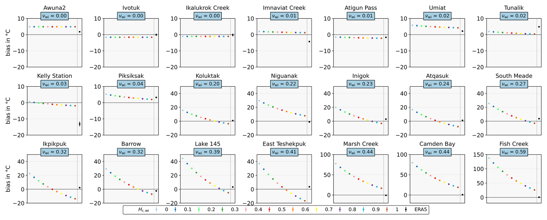
Figure 4 Bias per site for each H_r,wi used in the inversion. Each graph corresponds to one site. H_r,wi values are represented by a unique color and marker combination (see Legend) and are ranged from 0 to 1 with a 0.1 step on the x axis. The last point of each graph, in black, is obtained with T_g-ERA5. The y axis corresponds to the bias T_g−T_g-insitu. Note that the y-axis scale is variable. Each point is symbolized with error bars that correspond to the 5 %–95 % confidence interval. The sites are ordered in ascending order of water fraction (ν_wi in the light blue box).

4.2 T_g retrievals evaluation

4.2.1 T_g retrievals for sites with ν_wi≤0.04

The R, bias, and ubRMSD using MEM_G with H_r,gs = 0.8 and MEM_G+WI with H_r,wi = 1 were compared to T_g-ERA5 metrics in Fig. 5. For the sites with ν_wi≤0.04, when accounting for the water bodies with MEM_G+WI, we selected H_r,wi = 1 for the ice–water interface as it minimized the bias average of these sites (average = 0.6 °C). Each metric (in gray) is given with its confidence limits at 5 % (orange) and 95 % (blue). This representation enables us to show the dispersion of the metrics for all the considered sites. The R values of the retrieved T_g (median = 0.60 for both MEM_G and MEM_G+WI) were better than ERA5 (median = 0.51). Moreover, in the case of ERA5, the interquartile range was larger (Q1 = 0.33, Q3 = 0.55, range = 0.22) and the 5 % confidence limit dropped to negative values. All the biases are centered around zero (mean = 0.2 °C for MEM_G, 0.6 °C for MEM_G+WI and −0.8 °C for ERA5), and all the absolute biases were lower than 5 °C, except an outlier for ERA5 with a strong negative bias = −13.1 °C (Kelly Station, according to Fig. 3). The ubRMSD from both inversions (median = 2.1 °C for both MEM_G and MEM_G+WI) were significantly smaller than those from ERA5 (median = 3.9 °C).

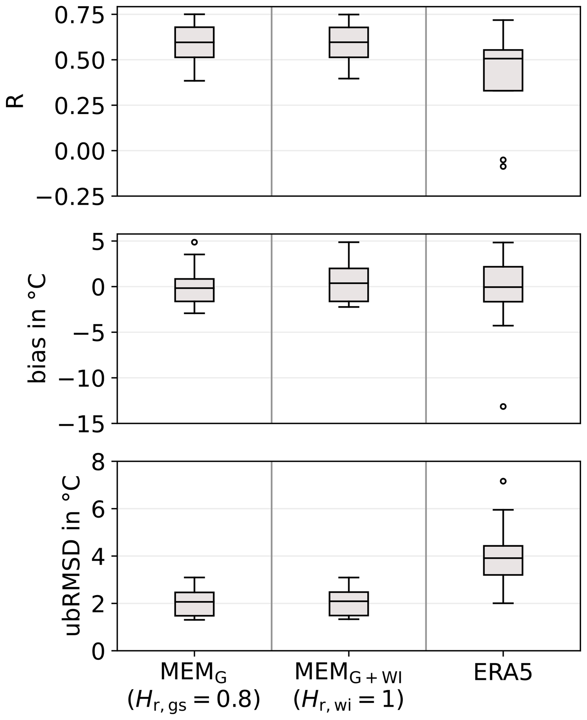
Figure 5 Summary statistics of R, bias and ubRMSD for sites with ν_wi≤0.04. The boxes show the median and interquartile range and whiskers show the 5 and 95 percentiles obtained from all the considered sites. The boxes correspond to the skill estimate (R, bias, or ubRMSD). The associated 5 % and 95 % CI are provided in Fig. B1. The x axis corresponds to the H_r,wi used in the inversion. The boxes are, respectively obtained from: MEM_G with H_r,gs = 0.8 (left), MEM_G+WI with H_r,wi = 1 (center) and ERA5 (right).

4.2.2 T_g retrievals for sites with $\mathrm{0.20}\le {\mathit{\nu }}_{\text{wi}}\le \mathrm{0.41}$

The overall R, bias and ubRMSD for MEM_G+WI with different H_r,wi are summarized in Fig. 6 with the corresponding MEM_G (with H_r,gs = 0.8) and ERA5 metrics. Similarly to Fig. 5, the boxes show the metric dispersion. The R values remained the same for all H_r,wi and equal to the R reached with MEM_G (median R = 0.21), but lower than ERA5 (median R = 0.62). The biases went more negative with increasing H_r,wi values. The bias was minimized for H_r,wi = 0.7 (Sect. 4.1.2), with a median value (0.2 °C) which was closer to zero than the bias with MEM_G (median = −13.0 °C) and with ERA5 (median = 2.3 °C). Yet, for bias, the interquartile range for H_r,wi = 0.7 (Q1 = −2.9 °C, Q3 = 2.8 °C, range = 5.7 °C) remained much larger than ERA5 (Q1 = 0.8 °C, Q3 = 3.2 °C, range = 2.4 °C), which meant that the bias remained higher for some of the sites. A wider range (Q1 = 4.4 °C, Q3 = 6.6 °C, range = 2.2 °C) was also observed for the ubRMSD for all the H_r,wi and MEM_G (Q1 = 3.7 °C, Q3 = 5.3 °C, range = 1.6 °C) with respect to ERA5 (Q1 = 3.2 °C, Q3 = 3.5 °C, range = 0.2 °C).

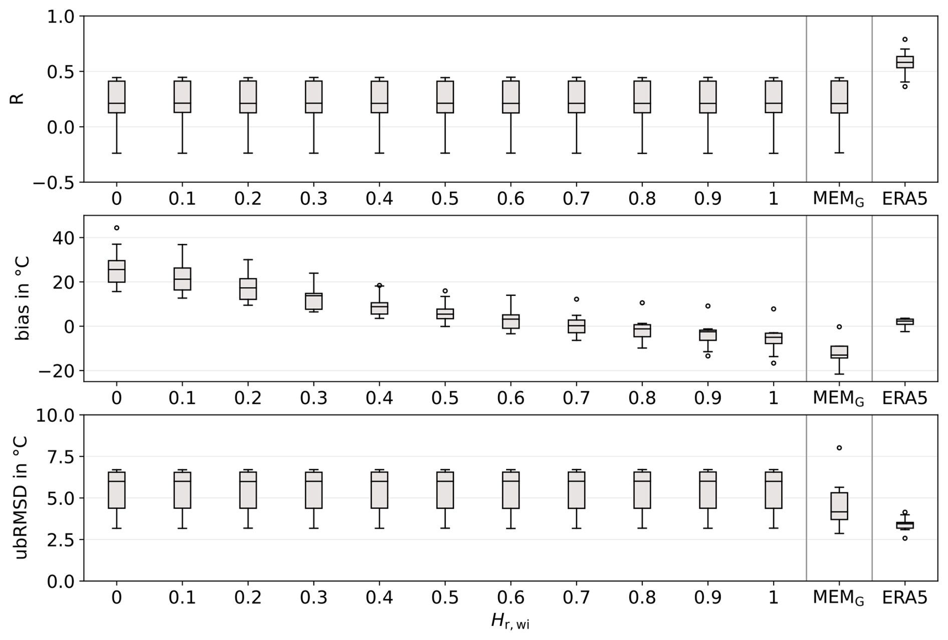
Figure 6 Summary statistics of R, bias and ubRMSD for sites with $\mathrm{0.20}\le {\mathit{\nu }}_{\text{wi}}\le \mathrm{0.41}$. The associated 5 % and 95 % CI are provided in Fig. B2. Boxes represent the site median and interquartile range (Q₃ - Q₁) and whiskers represent the 5 and 95 percentiles. The x axis corresponds to the H_r,wi used in the inversion. The rightmost boxes are obtained with ERA5.

5 Discussion

The SMOS satellite was originally designed to focus on SMOS, but the applications extend to biomass monitoring (Kerr et al., 2010, 2016b; Mialon et al., 2020) and soil freeze–thaw state (Rautiainen et al., 2014, 2016). Recently, cryosphere applications have been increasingly investigated (Leduc-Leballeur et al., 2020; Schwank et al., 2021; Holmberg et al., 2024). The synergy between theses studies should be further explored. For instance, producing T_g maps over the Arctic could complement the information from the freeze–thaw state products. In addition, this satellite-based approach is a first attempt to monitor the soil temperatures under the snowpack in the whole circumarctic permafrost area. Based on L-band observations of SMOS since 2010, continuing efforts in the long-term and operational permafrost state, monitoring would be made possible by the upcoming satellite missions CIMR and CryoRad (Donlon et al., 2023; Macelloni et al., 2018). Such soil temperature measurements would be highly beneficial for climate monitoring and carbon cycle modeling. Future work will look at integrating our approach to assimilation approaches such as the SMAPLv4 to improve soil temperature in winter and winter soil CO₂ emission.

The retrieval model parametrization evaluation showed clear contrasting results according to the water bodies fraction over sites; T_g retrievals outperformed ERA-5 when ν_wi≤0.04 but are mitigated when ν_wi≥0.20. Improvement of the T_g retrievals may be further explored with more complex modeling, auxiliary data or a 2-parameter inversion. Previous studies have shown the effects of ground permittivity and snow density to L-band BTs at theoretical, tower-based radiometer and satellite scales, Schwank et al. (2014); Lemmetyinen et al. (2016); Roy et al. (2017); Holmberg et al. (2024). We can expect the same for snow density and ground temperature. So a joint retrieval of T_g and snow density may remove some artifacts due to the snow signal in the retrieved T_g time series. However, additional prior information may be required to ensure inversion stability. In the high-latitude areas, the revisit time is short. For all the sites, the median value of the difference between T_g-insitu at days t and t+1 is 0.03 °C. This difference remains at 0.1 °C for a 3 d lag. Thus, T_g-insitu is very stable for short time range, which supports the thermal insulation of the snowpack. Considering a small temporal variation of T_g due to the snowpack thermal insulation, retrievals could be based on observations from multiple orbits (Konings et al., 2016). This could decrease the effect of the instrumental noise on the retrievals.

5.1 T_g retrievals under the snowpack for sites with ν_wi≤0.04

For sites with ν_wi≤0.04, correlation, bias and ubRMSD of the retrieval were superior to ERA5. A slightly negative bias was observed when the ν_wi was ignored (using the model MEM_G) but was successfully corrected with a model that accounts for snow and ice covered water bodies MEM_G+WI.

5.1.1 Frozen ground parametrization

We used a frozen ground permittivity of ε_frozen = 5 + 0.5 i, as defined by Hallikainen et al. (1985) and which was commonly used in various studies (Schwank et al., 2014; Kerr et al., 2020; Holmberg et al., 2024). The emission depth of L-band observations is usually associated with the first 5 cm of the ground (Schmugge, 1983). However, the emission depth varies with the ground state and texture, based on the ground attenuation constant α (${\mathit{\delta }}_{\mathrm{e}}=\mathrm{1}/\mathrm{2}\mathit{\alpha }$ Ulaby and Long, 2014), and consequently the ground complex dielectric constant ε_g. For ε_frozen = 5.0 + 0.5 i, the calculation based on Ulaby and Long (2014) shows that the associated emission depth δ_e≃ 15 cm. When it comes to frozen ground, the effective depth is still not well defined and it becomes even more complex with a snow layer on top of the ground. Rautiainen et al. (2012) estimated the emission depth of frozen ground at a maximum of 50 cm, but observed a T_B saturation only when reaching a 30 cm frost depth. By computing metrics for T_g-insitu at all the available depths for the sites with ν_wi≤0.04, we found that R was better than ERA5 (median = 0.51) for depth down to 30 cm (median range from 0.57 to 0.74) (Fig. 7). For in situ measurements down to 45 cm, the median absolute biases were smaller than 1.5 °C and the median ubRMSD were smaller than 2.5 °C. These results suggest that the sensitivity depth is in fact down to 50 cm or less. For deeper T_g-insitu, the correlation decreased to negative values (median R = −0.18 for depth = 120 cm). Note that for the period of this study (focused on T_g-insitu < −5 °C at 5 cm depth) the ground was fully frozen down to 50 cm for the 11 USGS sites that provide ground temperatures down to 120 cm. Due to potential shallow frozen soil, emissions from the underlying unfrozen soil should be taken into account in the early winter (Rautiainen et al., 2012). As observed by Schwank et al. (2004), the observed signal can encompass a contribution of the boundary between frozen and unfrozen soil, which was not taken into account in our modeling.

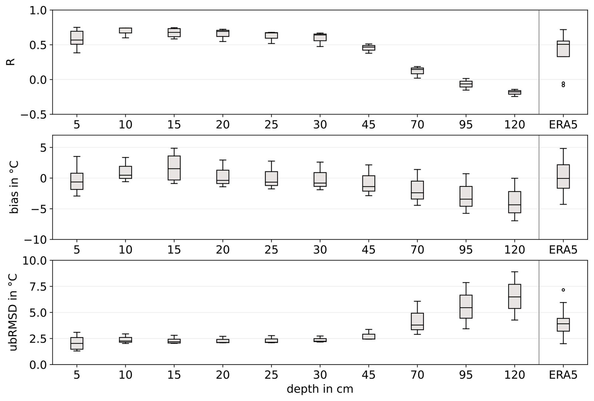
Figure 7 Summary statistics of R, bias and ubRMSD for sites with ν_wi≤0.04. The associated 5 % and 95 % CI are provided in Fig. 7. Boxes represent the site median and interquartile range (Q₃ - Q₁) and whiskers represent the 5 and 95 percentiles. The x axis corresponds to the in situ probing depths used for the validation. The extreme right boxes are obtained with ERA5 and T_g-insitu at 5 cm depth.

Concerning the ground surface parameters, the commonly used H–Q–N empirical model has been tuned for soil moisture (SM) and vegetation optical depth (VOD) retrievals in many studies (Parrens et al., 2017; Chaubell et al., 2020; Preethi et al., 2024). Hence, its parametrization should be optimized for T_g retrievals in the Arctic environment. We found the optimized set of values $H_{\mathrm{r},\text{gs}}=\mathrm{0.8}$, $Q_{\mathrm{r},\text{gs}}=\mathrm{0}$, $N_{\mathrm{r},\text{gs}}^{\mathrm{H}}=\mathrm{0}$, $=N_{\mathrm{r},\text{gs}}^{\mathrm{V}}=\mathrm{0}$ for the snow-ground interface, which is consistent with Holmberg et al. (2024). This parametrization depends on the chosen ground permittivity value. According to the Fresnel reflection coefficients (Eq. 2), increasing ground permittivity leads to a decrease of the emissivity. Using the H–Q–N model (Eq. 3), increasing H_r,gs means an increase of the emissivity. Thus, the soil parametrization requires a joint optimization of ε_g and H_r,gs.

We optimized H_r,gs based on a permittivity of a frozen ground value of ε_frozen = 5 + 0.5 i, but this value could be re-evaluated. The soil permittivity depends on the soil liquid water content and other characteristics (e.g., texture and bulk density). Based on a review of ground permittivity models (see Sect. 5.1.1), we investigated other potential values for frozen soil permittivity. For a frozen ground (T_g < −5 °C), we assumed the water to be completely frozen and thus SM negligible, i.e., SM≃ 0 m³ m⁻³ (Zhang et al., 2010; Mavrovic et al., 2023). Soil property information (clay fraction, sand fraction, soil organic content and bulk density) was extracted at each site location from the SoilGrids 250 m v2.0 database (Poggio et al., 2021) for the 0–5 cm soil layer (Table A1 in the appendices). The Soil Organic Carbon (SOC) content was very high at all the sites, as expected in the Arctic region, i.e 5 to 10 times higher than the global mean 40 g kg⁻¹ (according to SoilGrid v2.0), and so was the bulk density. Dielectric constant models like the commonly used Mironov model do not use the SOC information to compute the permittivity. It was first designed considering SM and clay content (Mironov et al., 2009). It was then further developed to use SM, T_sg (here set as −20 °C), and bulk density (Mironov et al., 2015). Park et al. (2017) was based on silt, clay, sand content and bulk density. Bircher et al. (2016) defined a soil permittivity model tailored for high organic content soils, whereas Park's model was updated to consider soil organic content (Park et al., 2019). The permittivities computed with these models for our sites are listed in Table A2 in the appendices. The obtained ε_frozen real parts went from 1 to 4, while the imaginary parts ranged from 0 to 0.1. This comparison of various permittivity models that depend on soil texture showed that the permittivity variability for frozen arctic soils was low and made legitimate the use of a fixed value for the ground permittivity. However, the obtained permittivities were significantly lower than ε_frozen = 5.0 + 0.5 i. This could be an evidence that SM > 0 m³ m⁻³, even in frozen ground conditions (T_g < −5 °C). In addition, a permittivity equal to ε_frozen = 5.0 + 0.5 i may result from a soil surface which was saturated with water at freezing time. But, as the Arctic soil shows high SOC and high bulk density (Table A1), it may not satisfy this water saturation condition. For the imaginary part of the permittivity, Mironov et al. (2015) showed a decrease with decreasing temperatures. In situ measurements of frozen ground permittivity could be valuable, simultaneously with tower-based radiometer observations in the Arctic tundra environment. Some probes seem efficient for this task, such as the one described in Gélinas et al. (2025). Using a constant permittivity, calculated under the assumption of a homogeneous ground, is a practical solution for our model, as it reduces the number of free parameters and auxiliary data. However, dielectric mixing models enable to characterize heterogeneous materials (Ulaby and Long, 2014) and could better fit the Arctic soils local behavior.

5.1.2 Effects of the snow layer

Snow cover was present for all ground temperature observations used in T_g retrievals (i.e., the observed snow depth was above 10 cm), motivating the use of a snow layer in the MEM model. Lemmetyinen et al. (2016) and Roy et al. (2017) suggested that snow emissions at L-band are related to the bottom 10 cm of the snow layer. The typical Arctic snow profile consists of a dense wind slab of high density (ρ≃ 300–400 kg m⁻³) but with a depth hoar underneath with lower density (ρ≃ 250 kg m⁻³) (Sturm et al., 1995). However, the impact in terms of ε_s is low in the model of Wiesmann and Mätzler (1999) and hence, we used (ε_s(ρ = 300 kg m⁻³) ≃ 1.5 and ε_s(ρ = 250 kg m⁻³) ≃ 1.4) in the present study. In addition, our model does not account for the inclusion of ice crusts in the snowpack (e.g., after rain-on-snow (ROS) events) (Bartsch et al., 2023), nor low vegetation (e.g., shrubs or mosses) that could be observed in the tundra environment (Royer et al., 2021a) and might add complexity to the snowpack microwave emission. In fact, Roy et al. (2015) observed a decrease in horizontal polarization as the impact of ice crust formation, but Roy et al. (2018) underlined the difficulty of modeling and quantifying such event at L-band. As for the vegetation, multiple effects may mitigate the T_g. The presence of shrubs leads to a snow accumulation with a lower density than on herbaceous areas, which means more thermal insulation from the snowpack (Grünberg et al., 2020; Liston et al., 2002). However, Domine et al. (2022) also observed thermal exchanges between air and soil through the branches. As these effects are observed at local scale, it is difficult to model it at the SMOS scale (≃ 40 km). Various temporal matching between in situ measurements T_g-insitu and the retrieved T_g were tested (not shown): closest measurement to the satellite overpass time (Catherinot et al., 2011) or daily maximum, minimum (Jones et al., 2007) or mean. The metrics remained similar because we observed very few daily variations of T_g due to the snow insulation effect.

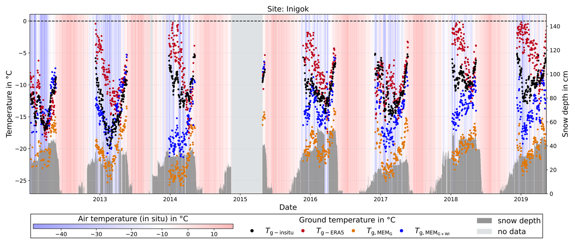
Figure 8 Time series of the ground temperatures (in °C, left axis) at Inigok from 2012 to 2020: T_g-insitu (in black), $T_{\mathrm{g},{\text{MEM}}_{\mathrm{G}}}$ (in orange), $T_{\mathrm{g},{\text{MEM}}_{\mathrm{G}+\text{WI}}}$ (in blue) and T_g-ERA5 (in red). The snow depth (in cm, right axis) is displayed as dark gray bar plots. In the background, stripes from blue to red account for the in situ air temperature (in °C).

5.2 T_g retrievals under the snowpack for sites with ν_wi≥0.20

For sites with $\mathrm{0.20}\le {\mathit{\nu }}_{\text{wi}}\le \mathrm{0.41}$, the retrievals showed a strong negative bias when ignoring the snow and ice covered water bodies with MEM_G. We corrected the bias with the model MEM_G+WI accounting for water body contribution by optimizing the H_r,wi parameter. A single H_r,wi value did not suit all the sites. Validating T_g retrievals for sites with water body fractions between 0.04 and 0.20 may help to understand the water body effects in the retrievals and how to account for them. For sites with ν_wi≥0.44, the bias was larger with MEM_G+WI than with MEM_G. In fact, the bias could already be minimized using an appropriate H_r,gs. However, the correlation remained poor for these sites (R<0.3). For ERA5, the bias median was larger for sites with ν_wi≥0.20 (median = 1.0 °C) than for sites with ν_wi≤0.04 (median = −0.1 °C). For sites with higher biases (namely, Niguanak, Marsh Creek, Camden Bay and Fish Creek), no correlation could be made with surface characteristics, such as land cover (Table 1) and soil content (Table A1). However, we noticed that those sites correspond to coastal pixels, i.e., made of BT measured on the continent and the ocean. Kerr et al. (2020) highlighted the retrieval difficulties for coastal BT that result from mixed pixels. In fact, the observation geometry variations that lead to various water fractions are not taken into account in the MEM.

5.2.1 Effects of the snow and ice covered water bodies

We used the water fraction for a 40 km resolution, but Kerr et al. (2020) showed that a working area of approximately 123 km × 123 km is required to capture all the microwave signal that contributes to the SMOS observed BT. In fact, due to the multiple observation angles, the size and shape of the elliptical footprint vary. Using an average single round buffer for all the angles is a potential error source. For sites located near the coast, the nearby presence of the ocean is non-negligible. The considered water body areas may also vary over time. Dynamic water maps could improve the T_B correction, even more if they provide us with information on the water state (e.g., frozen, snow and ice covered, etc.). The water bodies greatly affect the passive microwaves observations in summer in the Arctic area (Ortet et al., 2024). Including water bodies in the MEM in winter is even more difficult because even if their surface is fully covered with ice, they may not be completely frozen in depth (Lemmetyinen et al., 2011). We tested various modeling configurations for the water bodies (ice only, liquid water only, ice on top of liquid water with a smooth interface, not shown). None were fully successful, but introducing the H_r,wi parameter worked better. Indeed, it represents the surface roughness at the ice–water interface, which is not flat and significantly affects microwave observations. Yet, different models should be applied depending on water body characteristics (e.g., depth) as shallower lakes could freeze down to the bottom or sea ice may be formed on the coastal areas.

5.2.2 Analysis of a site with high water fraction (Inigok)

Figures 4 and 6 show that using a unique H_r,wi for all the sites does not ensure fully optimized T_g. To better understand the possible impact of snow and ice covered water bodies and model configuration, we present the Inigok site with a high water fraction of ν_wi=0.23. Figure 8 shows varying performance of the time series of $T_{\mathrm{g},{\text{MEM}}_{\mathrm{G}}}$, $T_{\mathrm{g},{\text{MEM}}_{\mathrm{G}+\text{WI}}}$ and T_g-ERA5 compared to T_g-insitu. The $T_{\mathrm{g},{\text{MEM}}_{\mathrm{G}}}$ time series showed a negative bias that was well corrected in the $T_{\mathrm{g},{\text{MEM}}_{\mathrm{G}+\text{WI}}}$ time series. The T_g-ERA5 time series did not show a systematic bias with the T_g-insitu time series. However, the ERA5 dynamic was quite different from the in situ measurements. While T_g-insitu and T_g seemed linked to air temperature when it rises above −10 °C (e.g., in early 2014), but with a lag. This was not observed for T_g-ERA5, while it appeared in the retrieved $T_{\mathrm{g},{\text{MEM}}_{\mathrm{G}}}$ and $T_{\mathrm{g},{\text{MEM}}_{\mathrm{G}+\text{WI}}}$. This could be linked to wet snow events, that increase the snowpack thermal conductivity and consequently the link between air temperatures and T_g. They also challenge the snowpack transparency hypothesis (Kumawat et al., 2022), that could no longer be valid, and could lead to an increase in the retrieved T_g values. Using MEM_G or MEM_G+WI did not affect the time series dynamic, as shown by the similar R and ubRMSD in Fig. 6. However, a strong interannual difference is observed. In winter 2014, we found R = 0.46 for T_g-ERA5, while we obtained R = 0.29 for both $T_{\mathrm{g},{\text{MEM}}_{\mathrm{G}}}$ and $T_{\mathrm{g},{\text{MEM}}_{\mathrm{G}+\text{WI}}}$ (see Fig. C1 in the appendices). By contrast, in winter 2019, a correlation of R = −0.03 is obtained with ERA5, while R = 0.61 using MEM_G or MEM_G+WI. These discrepancies between years suggest that ice conditions change throughout the years and further ice parametrization would be needed to obtain satisfactory T_g retrievals for scenes with high water body fractions.

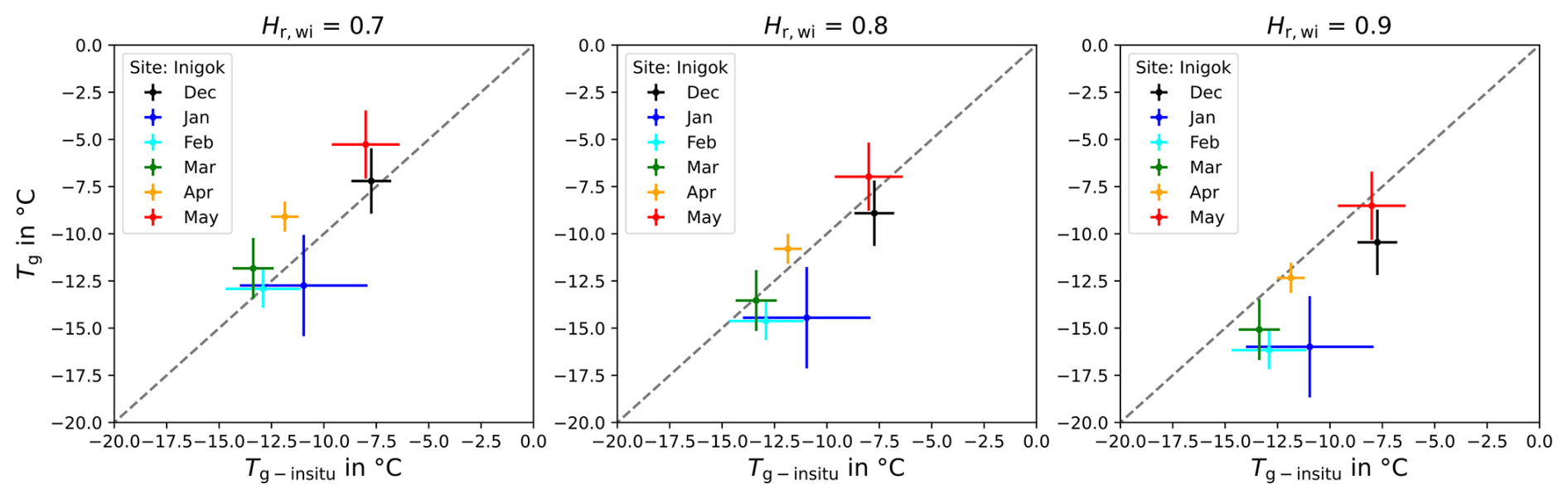
Figure 9 Scatter plots of the retrieved monthly average T_g (in °C) against in situ averaged T_g-insitu (in °C) at the Inigok site from December 2016 to May 2017. The error bars show the standard deviation of the retrieved and measured temperatures. H_r,wi values used in the inversion are 0.7 (left), 0.8 (middle), and 0.9 (right). The gray dashed line corresponds to the 1:1 identity line.

The similarities of behaviors of in situ and retrieved time series also varied during a single season. Figure 9 focuses on the retrievals using MEM_G+WI with different H_r,wi at Inigok from December 2016 to May 2017. This period corresponds to the winter season with best correlation according to Fig. C1 (R = 0.74). The retrieved T_g and T_g-insitu were averaged per month and plotted with their standard deviation. Each graph of Fig. 9 corresponds to a different H_r,wi used in the modeling. The difference between the monthly averaged T_g and the monthly averaged T_g-insitu is denoted $\mathrm{\Delta }\stackrel{\mathrm{‾}}{T}$. December ($\mathrm{\Delta }\stackrel{\mathrm{‾}}{T}$ = −0.5 °C), January ($\mathrm{\Delta }\stackrel{\mathrm{‾}}{T}$ = −1.8 °C) and February ($\mathrm{\Delta }\stackrel{\mathrm{‾}}{T}$ = 0 °C) T_g are in good agreement with T_g-insitu for H_r,wi = 0.7. However, in March, H_r,wi = 0.8 provides better results ($\mathrm{\Delta }\stackrel{\mathrm{‾}}{T}$ = −0.2 °C). The best H_r,wi is 0.9 for April ($\mathrm{\Delta }\stackrel{\mathrm{‾}}{T}$ = −0.5 °C) and May ($\mathrm{\Delta }\stackrel{\mathrm{‾}}{T}$ = −0.5 °C). This suggests a possible evolution of the ice conditions throughout the winter that affects the ice–water surface rugosity and T_g inversion. This is in agreement with synthetic aperture radar (SAR) studies (Duguay and Lafleur, 2003; Murfitt et al., 2023) which take into account roughness parameters over lakes to represent the impact of the roughness at the water–ice interface on microwave signal. Murfitt et al. (2023) linked the water–ice interface roughness with the growth of tubular bubbles during ice formation, leading to higher roughness. Slushing water in ice cracks at the end of the freezing season induces more complexity than our three horizontal layer modeling for water bodies (Adams and Lasenby, 1985). Ground-based radiometric observations would be highly beneficial to better understand the seasonal effect of water–ice interface roughness on T_B in Arctic regions. Such observations may also help the development of a more complex model to better describe the L-band emissions of the circumarctic lakes and their variations through the seasons.

6 Conclusions

This study aimed to expand the previous studies on L-band passive microwave modeling and ground-based observations of snow-covered scenes by retrieving ground temperatures from satellite measurements in winter conditions. Our approach is based on SMOS L-band observations from 2012 to 2019. Two MEM configurations were explored to retrieve the T_g below the snowpack in the Arctic: one considering a homogeneous scene (MEM_G) and another one correcting the scene for the snow and ice covered water body fraction (MEM_G+WI). Values of T_g retrieved with both MEM were validated with in situ measurements of 21 sites across Northern Alaska and compared to T_g-ERA5. Several conclusions can be drawn from our results:

• T_g under the snowpack can be retrieved from SMOS observations with a relatively simple MEM and limited auxiliary data.

• For sites with low water fraction (≤ 0.04), values of T_g were retrieved with a median correlation R of 0.60 and a median bias of −0.2 °C. For the same sites, the ERA5 median R was 0.51 and median bias was −0.8 °C.

• For sites with a higher water fraction (≥ 0.20), ignoring the water fraction (MEM_G) leads to strong negative biases. The bias can be reduced using an ice–water roughness parameter H_r,wi, but correlation with in situ data remains low (< 0.5 and worse than ERA5).

• Further work needs to be done to assess the impact of the snow and ice covered water bodies on L-band T_B evolving through the winter season.

With its launch in 2010, SMOS has offered observations for almost 15 years to this day. Producing T_g maps over the Arctic for the whole period would improve monitoring of the permafrost state in space and time and would be highly beneficial for carbon models.

Appendix A: Soil properties

Table A1 Study sites soil characteristics at 0–5 cm extracted from SoilGrids 250 m v2.0 database (Poggio et al., 2021).

Mironov et al. (2009)Mironov et al. (2015)Park et al. (2017)Park et al. (2019)

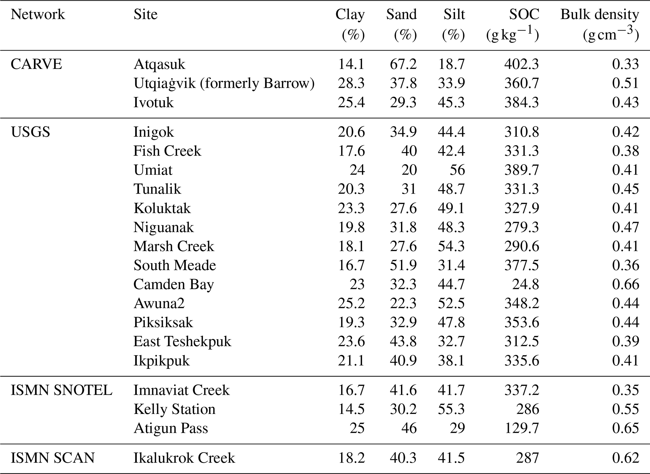
Table A2 Frozen soil permittivity ε_frozen obtained from various dielectric constant models. No unfrozen water is considered, i.e., SM = 0 m³ m⁻³. When needed, the other soil properties are from SoilGrid 250 m v2.0 (Poggio et al., 2021) (Table A1). Note that the sign before the imagery part depends on different conventions. i is defined as an imaginary number, e.g. $i^{\mathrm{2}}=-\mathrm{1}$.

Appendix B: Results – figures with confidence intervals

The Figs. B1–B3 below are, respectively, similar to the Figs. 5–7 but with the confidence intervals (CI) of each metric. The 5 % and 95 % CI are, respectively, represented in orange and blue, the metric in gray. As for each metric, the CI distribution of all sites is represented with a boxplot.

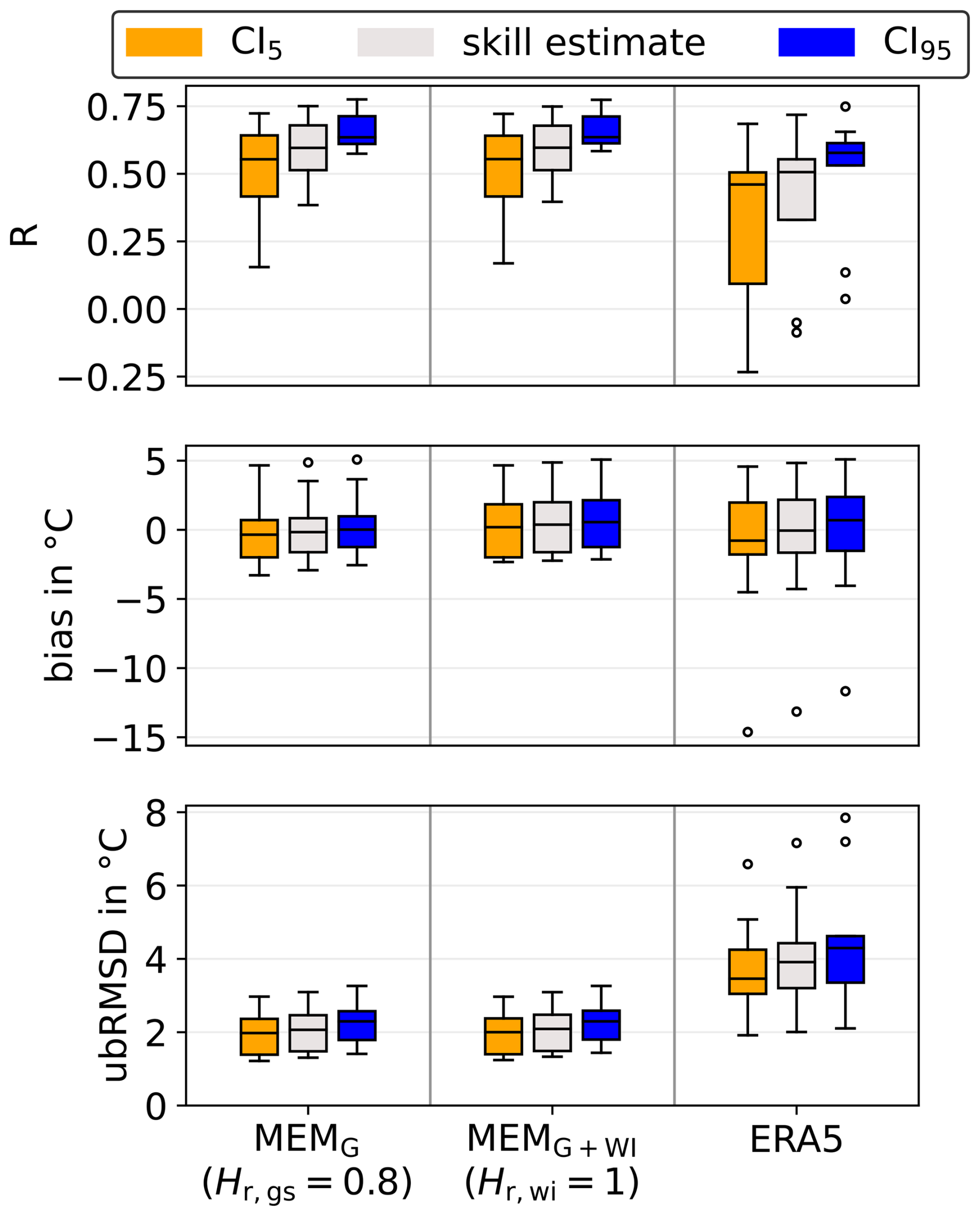
Figure B1 Summary statistics of R, bias and ubRMSD for sites with ν_wi≤0.04. The boxes show the median and interquartile range and whiskers show the 5 and 95 percentiles obtained from all the considered sites. The gray box corresponds to the skill estimate (R, bias, or ubRMSD). Respectively, the orange and blue boxes correspond to the associated 5 % and 95 % confidence interval limits obtained from all the considered sites. The x axis corresponds to the H_r,wi used in the inversion. The boxes are, respectively obtained from: MEM_G with H_r,gs = 8 (left), MEM_G+WI with H_r,wi = 1 (center) and ERA5 (right).

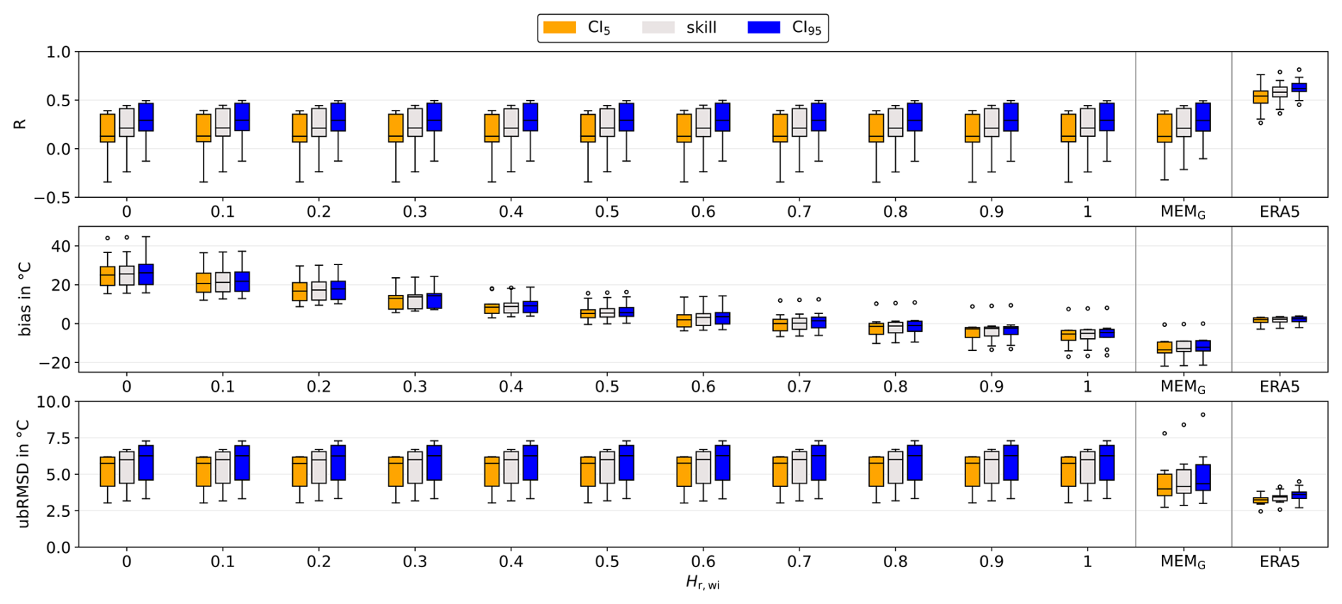
Figure B2 Summary statistics (in gray) of R, bias and ubRMSD and their 5 % (in orange) and 95 % (in blue) confidence intervals for sites with $\mathrm{0.20}\le {\mathit{\nu }}_{\text{wi}}\le \mathrm{0.41}$. Boxes represent the site median and interquartile range (Q₃ - Q₁) and whiskers represent the 5 and 95 percentiles. The x axis corresponds to the H_r,wi used in the inversion. The rightmost boxes are obtained with ERA5.

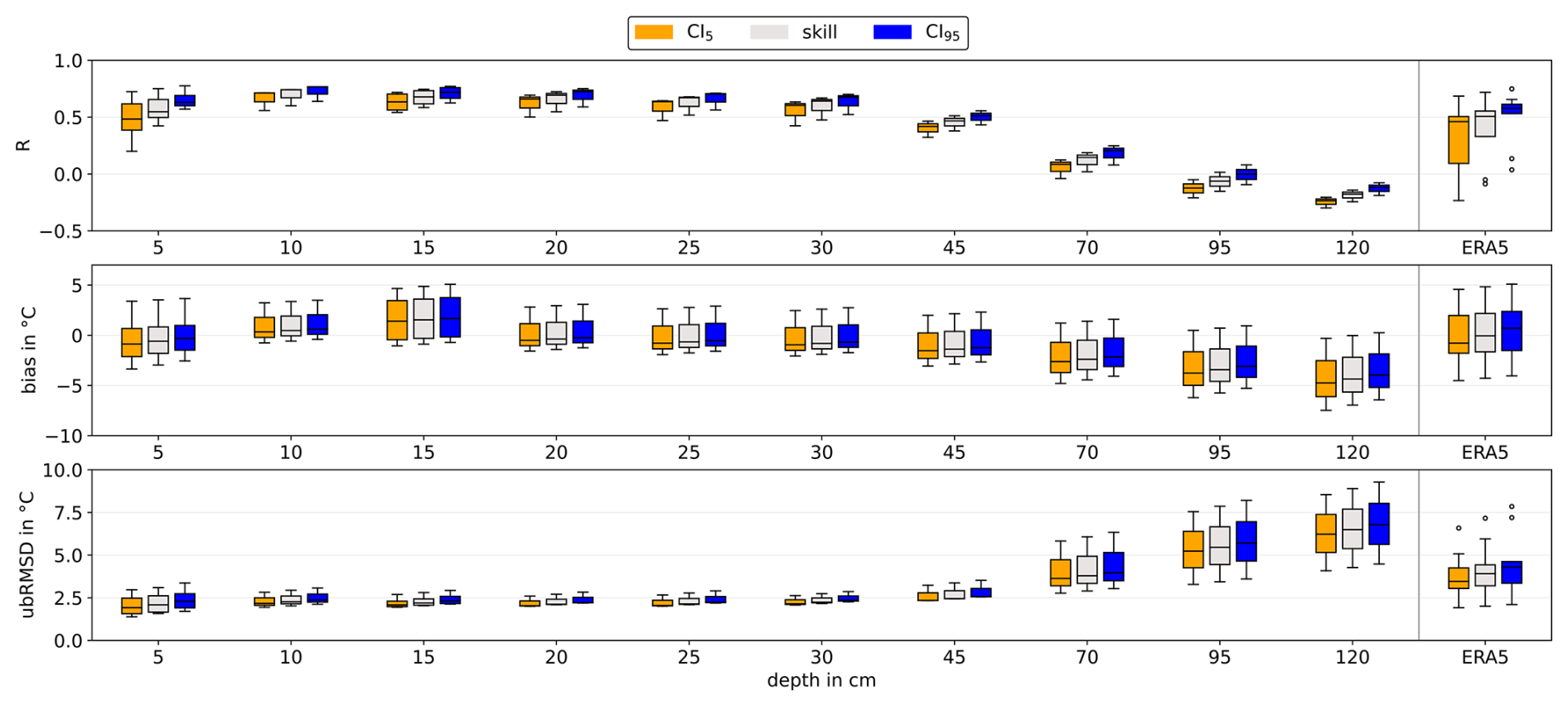
Figure B3 Summary statistics (in gray) of R, bias and ubRMSD and their 5 % (in orange) and 95 % (in blue) confidence intervals for sites with ν_wi≤0.04. Boxes represent the site median and interquartile range (Q₃ - Q₁) and whiskers represent the 5 and 95 percentiles. The x axis corresponds to the in situ probing depths used for the validation. The extreme right boxes are obtained with ERA5 and T_g-insitu at 5 cm depth.

Appendix C: Case study – Inigok

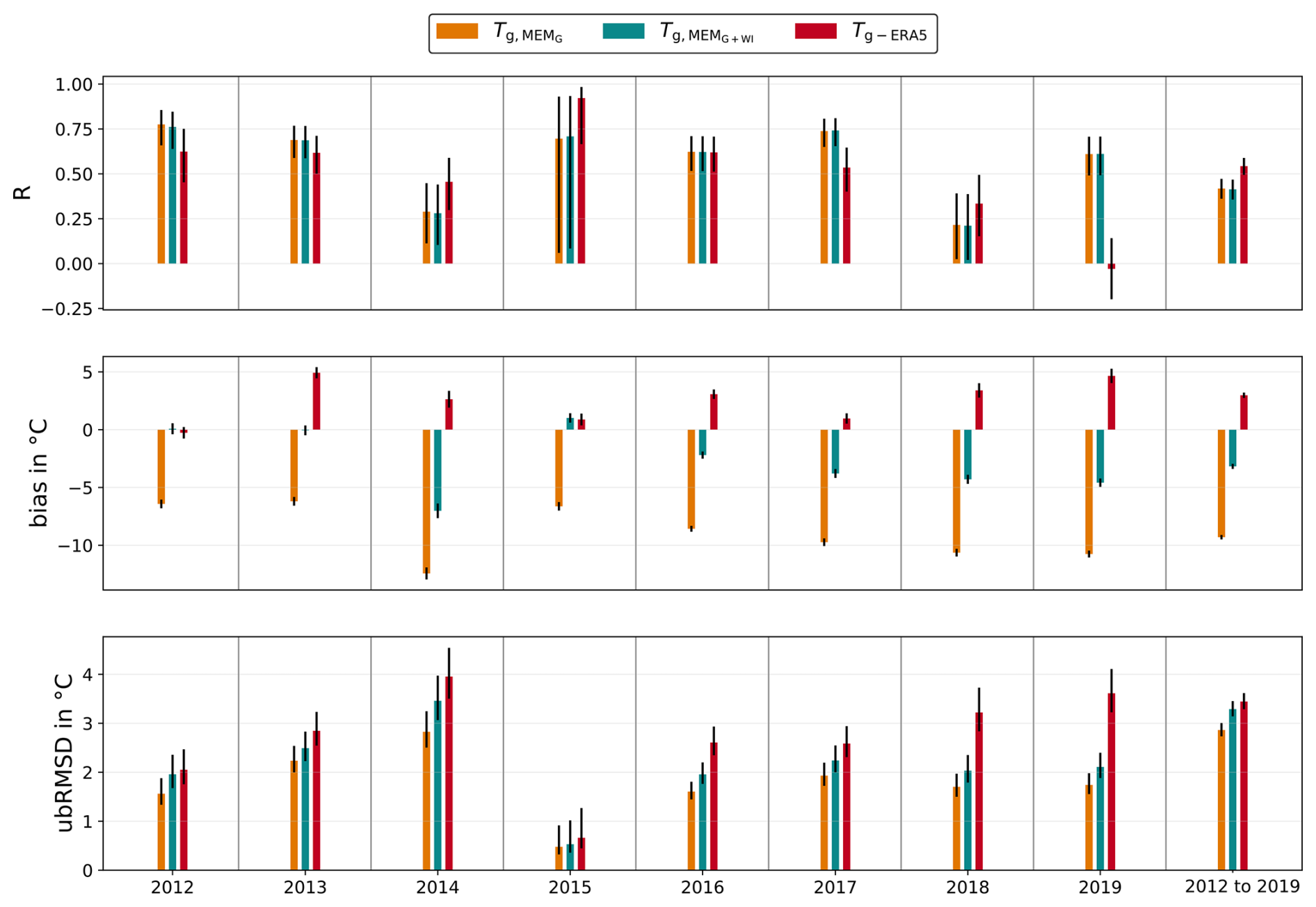
Figure C1 Yearly metrics obtained at Inigok from 2012 to 2020: $T_{\mathrm{g},{\text{MEM}}_{\mathrm{G}}}$ (in orange), $T_{\mathrm{g},{\text{MEM}}_{\mathrm{G}+\text{WI}}}$ (in blue) and T_g-ERA5 (in red). R, bias and ubRMSD are plotted as bar plots, with error bars accounting for their 5 % and 95 % confidence intervals. On the far right, we show the global metrics obtained for the whole time series.

Appendix D: Summarizing performances

Table D1 Biases in °C for all sites (lines) and all H_r (columns). The last column gathers scores from ERA5. The sub-table on top corresponds to the model MEM_G and the one below to the model MEM_G. The smallest bias obtained with MEM_G or MEM_G+WI per site (i.e., line) is in bold.

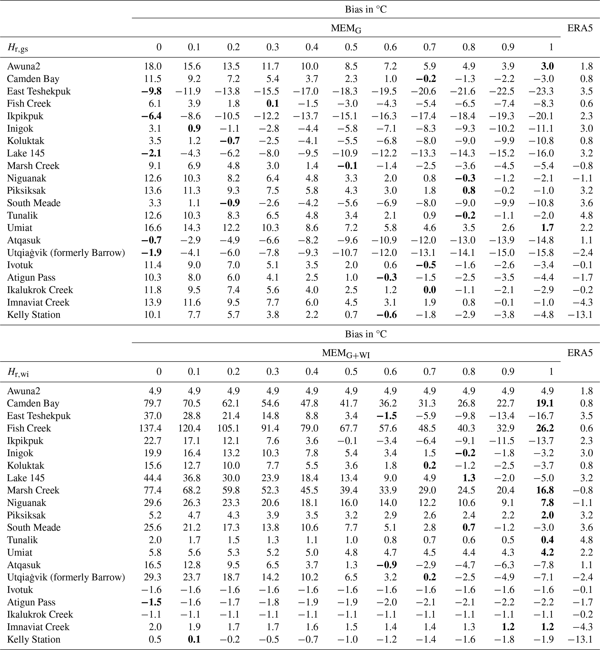
Table D2 R for all sites (lines) and all H_r (columns). The last column gathers scores from ERA5. The sub-table on top corresponds to the model MEM_G and the one below to the model MEM_G.

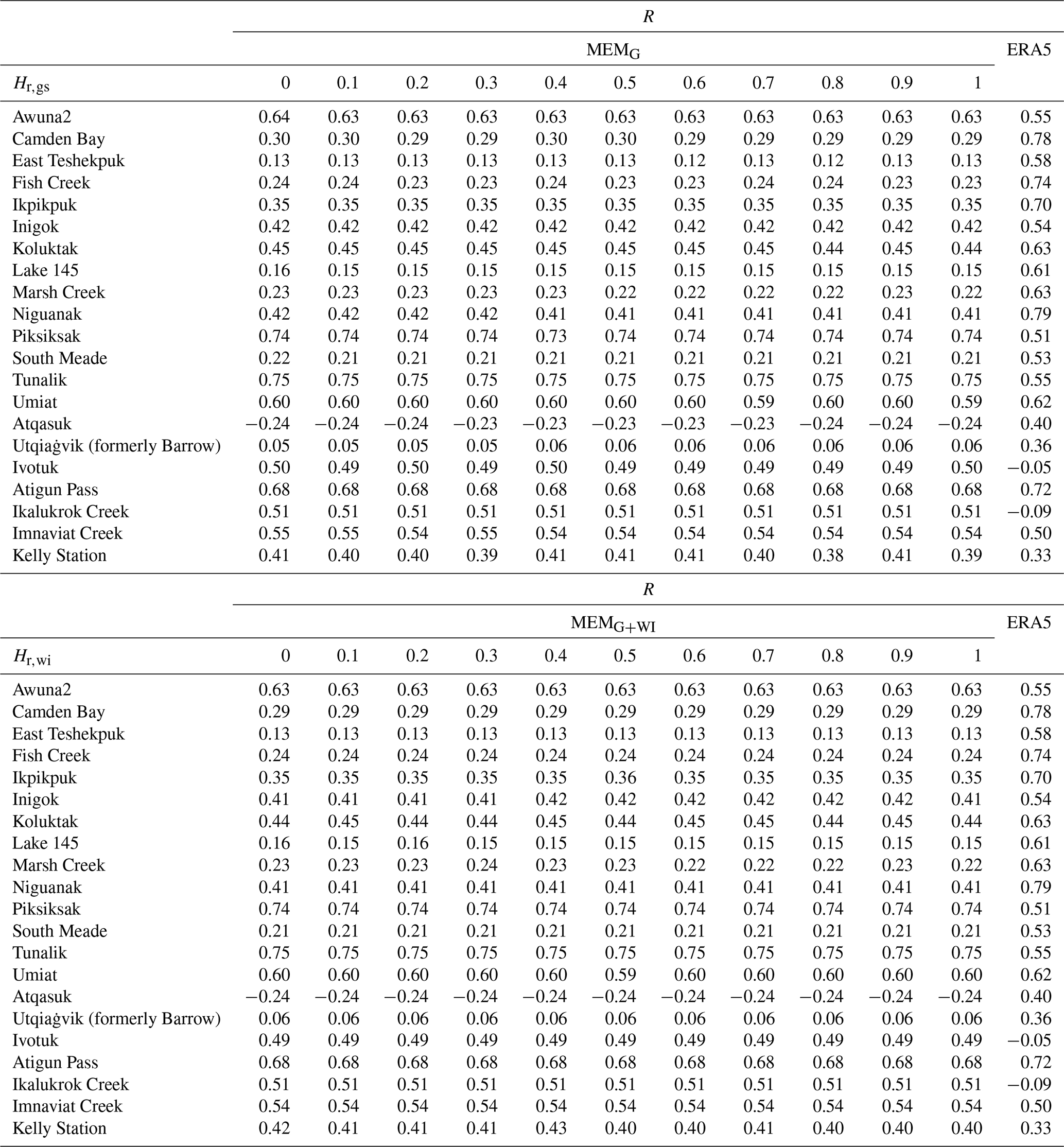
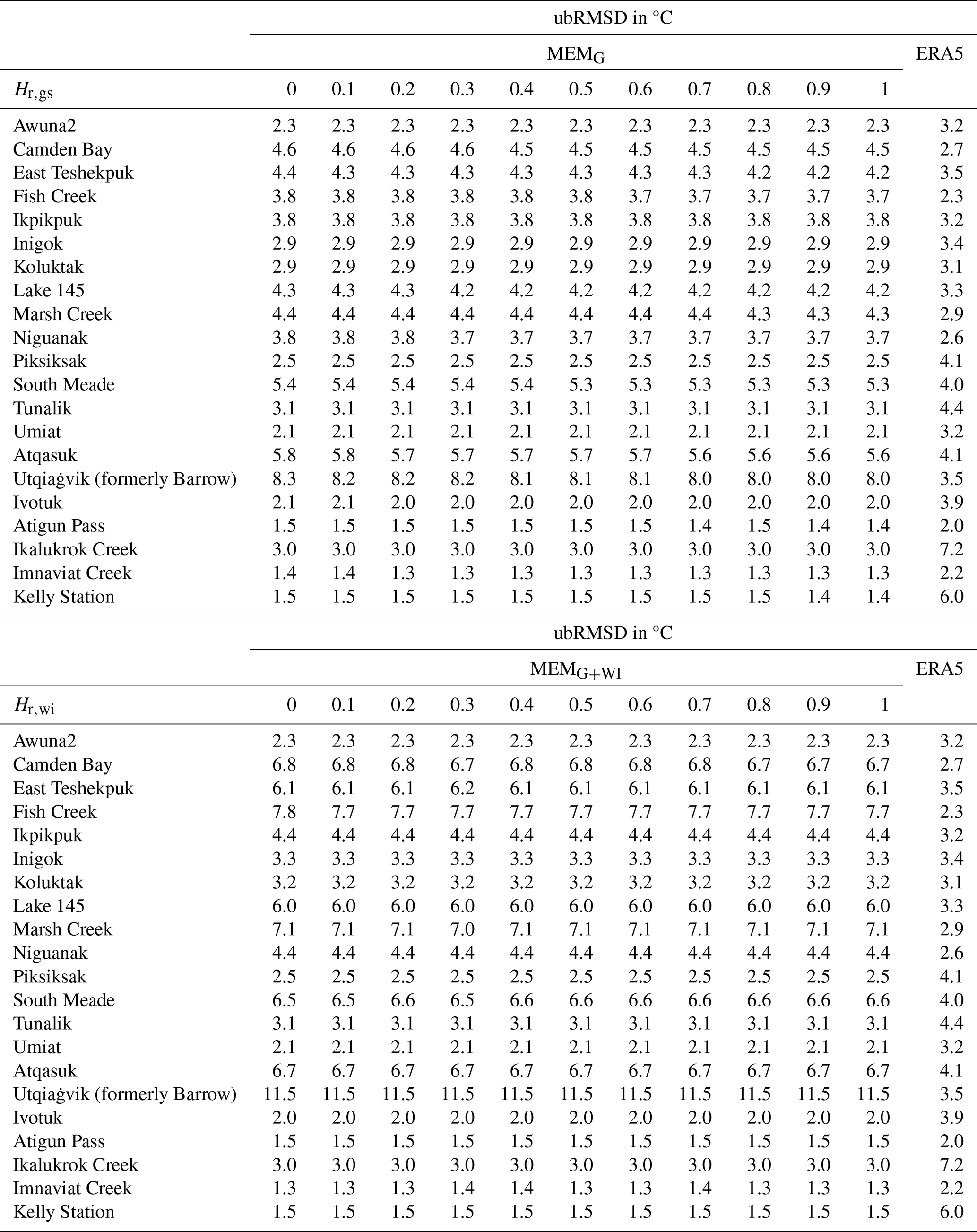
Table D3 ubRMSD in °C for all sites (lines) and all H_r (columns). The last column gathers scores from ERA5. The sub-table on top corresponds to the model MEM_G and the one below to the model MEM_G.