ITS_LIVE global glacier velocity data in near-real time

Glaciers and ice sheets cover some 15 million square kilometers of the Earth's surface, shaping continental landscapes and modifying climate on a global scale. Recent decades of atmospheric and oceanic warming have induced rapid glacier loss worldwide that has caused sea level rise, flooding, changes to Earth's overall energy balance, and changes in water resources. Accounting for the total impact of glacier change requires observations on a global scale, and planning for future change will require improved understanding of the physical controls that govern glacier change. One key factor that dictates glacier and ice sheet loss is changes in rates of ice flow, the physics of which remain poorly constrained. Our physical understanding of ice flow can be advanced with high-resolution monitoring of glacier flow in near-real time. Automated tracking of glacier flow from space became possible with the launch of Landsat 4 in 1982. Since then, an increasing number of optical and radar satellite sensors have provided a full decade of year-round, global data coverage. This recent plethora of data has introduced new challenges for efficiently processing such large and myriad data streams in a standardized manner with low latency. Here we present the NASA Making Earth System Data Records for Use in Research Environments (MEaSUREs) Inter-mission Time Series of Land Ice Velocity and Elevation (ITS_LIVE) global glacier velocity dataset, which is freely available to the public and is currently on major release version 2.0. ITS_LIVE has computed surface velocities using every, excluding those with high cloud cover, available image from Landsat 4 through Landsat 9 as well as Sentinel-1 and Sentinel-2, creating a global glacier velocity record of over 36 million image pairs dating back to 1982. The ITS_LIVE processing chain automatically performs feature tracking on more than 20 000 image pairs per day, within minutes of image availability, and will soon include data from Sentinel-1C and NASA-ISRO SAR Mission (NISAR) satellites. This paper describes the ITS_LIVE processing chain and provides guidance for working with the cloud-optimized velocity data it produces.

1 Introduction

In recent decades, glacier velocity observations have revealed a complex and evolving landscape of ice flow that spans the globe and shapes the Earth's surface and human behavior. In the distant past, glacier flow carved great fjords, such as those of Greenland, where fishing and tourism along the coast represent major pillars of the country's modern economy (Bendixen et al., 2019). In modern times, satellite observations have revealed glacier acceleration that has increased ice discharge to the ocean and raised sea levels (IPCC, 2023; Otosaka et al., 2023), impacted ocean circulation and primary productivity (Li et al., 2024; Perner et al., 2019), increased risk of flooding (Cook et al., 2016; Bazai et al. 2021; Rounce et al., 2017), modified stream flows (Pritchard et al., 2019; Ultee et al., 2022), and shifted Earth's energy balance (Hansen et al., 2011; Sicart et al., 2008). Understanding and accounting for the myriad impacts of global changes in ice dynamics have been made possible by global satellite data coverage, and as we face a future of certain climate change, preparing for the impacts of glacier variability will require near-real-time monitoring of glacier dynamics on a global scale.

The use of satellite images to measure glacier velocity began in the 1980s with manual identification of persistent features (e.g., crevasses) that were displaced between pairs of satellite images (e.g., Lucchitta and Ferguson, 1986; Whillans and Bindschadler, 1988). By the 1990s, template matching algorithms (i.e., normalized cross-correlation) were developed to systematically measure displacement fields from image pairs for investigations of glacier flow (Bindschadler and Scambos, 1991; Scambos et al., 1992), and that work has since led to the development of several open-source software packages for feature tracking, including COSI-Corr (Leprince et al., 2007), MATLAB-based ImGRAFT (Messerli and Grinsted, 2015), Python-based PyCorr (Fahnestock et al., 2016), Glacier Image Velocimetry (GIV: Van Wyk de Vries and Wickert, 2021), and the autonomous Repeat Image Feature Tracking (autoRIFT) package (Gardner et al., 2018; Lei et al., 2021) used to generate the ITS_LIVE data described in this paper. After years of algorithm development and remote sensing data collection, a few major efforts have generated large-scale ice velocity mosaics that have each enabled a new wave of advancements in glaciological observation and modeling.

One of the first large-scale ice velocity mapping projects used RADARSAT synthetic aperture radar (SAR) data to map the flow of the Greenland Ice Sheet (Joughin et al., 2010), and soon after, multiple years of SAR data were stitched together to create a nearly complete map of the flow of the Antarctic Ice Sheet (Rignot et al., 2011). In the years that followed, ice-sheet-wide mosaics became available at annual (Gardner et al., 2022; Joughin, 2023a; Mouginot et al., 2017) and subannual (Joughin, 2022, 2023b; Solgaard and Kusk, 2022) intervals, and image-pair-level velocity data were made available for the full Landsat 8 record via GoLIVE (Scambos et al., 2016) and later ITS_LIVE (Gardner et al., 2022). Beyond the ice sheets, glacier velocity data have been generated globally for a single snapshot in time (Millan et al., 2021), as annual mosaics (Gardner et al., 2022), and as displacement fields measured in individual image pairs from various satellite sensors (Gardner et al., 2022; Scambos et al., 2016). The large and rapidly growing volume of remote sensing data now far exceeds the storage and processing capabilities of any laptop computer or local workstation, meaning modern, cloud-optimized approaches for velocity data generation and storage will be essential to usher in the next generation of glaciological advancement (López et al., 2023). The cloud-native processing chain developed for ITS_LIVE version 2.0 is described below.

2 Processing system

Due to the sheer volume of data and intensive processing needs, ITS_LIVE decided to adopt a cloud-first approach to data processing and access. The ITS_LIVE processing chain is an Amazon Web Service (AWS) cloud-native application. It is composed of three major components: (1) ITS_LIVE Monitoring that watches for new satellite image acquisitions, (2) Hybrid Pluggable Processing Pipeline (HyP3) ITS_LIVE that orchestrates the processing of image pairs, and (3) HyP3-autoRIFT that processes image pairs and publishes them to the ITS_LIVE AWS OpenData Simple Storage Service (S3) bucket.

2.1 ITS_LIVE Monitoring

The ITS_LIVE Monitoring stack (Kennedy et al., 2025a) uses an event-driven architecture to listen for new input satellite data products to be published, find new images to use for velocity estimation, and submit qualifying image pairs (criteria described in Sect. 3) for processing to HyP3 ITS_LIVE (Sects. 2.2–3). Figure 1 illustrates the data flow for Landsat images.

For Landsat 8/9 data, ITS_LIVE Monitoring subscribes to the USGS's Simple Notification Service (SNS) topic, which broadcasts messages describing newly available Landsat data. All level 1, tier 1 and 2 products from Collection 2 are placed into an AWS Simple Queue Service (SQS), which then triggers an AWS Lambda that evaluates if the corresponding scene qualifies for processing based on the scene's metadata in the USGS SpatioTemporal Asset Catalog (STAC). Each qualifying scene is used as a reference scene, the USGS STAC is searched for qualifying secondary scenes, and each reference and secondary scene pair is submitted to HyP3 ITS_LIVE for processing. New velocity granules are published to the its-live-data AWS S3 bucket by HyP3 ITS_LIVE, typically within 15 min of a new Landsat data product being broadcast.

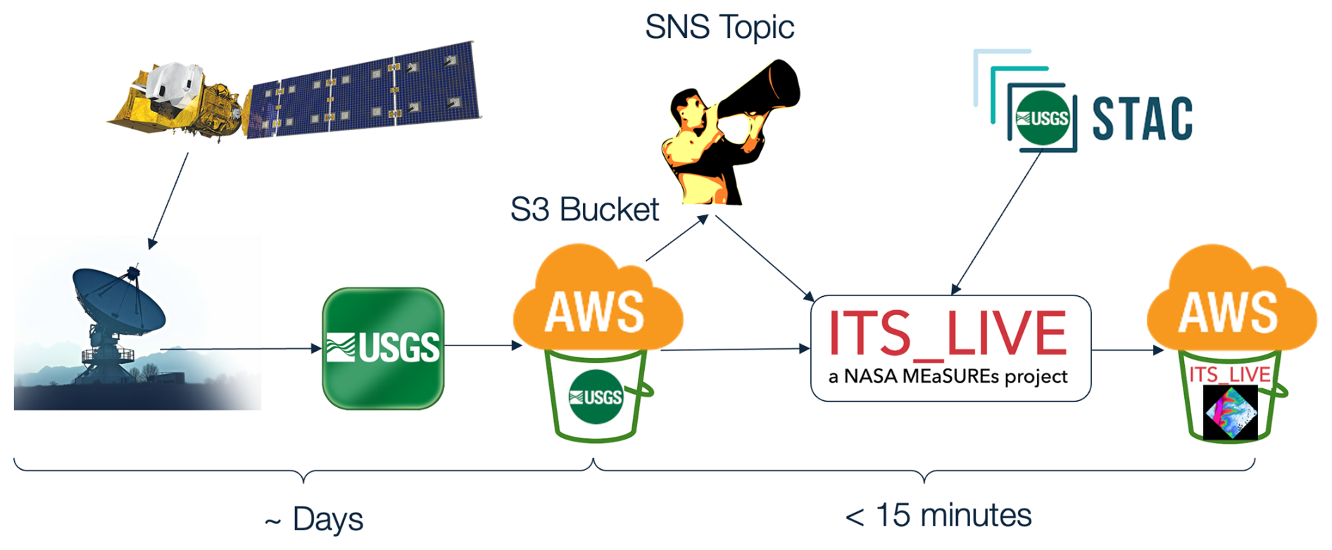
Figure 1 Landsat data flow, from acquisition to ITS_LIVE velocity. Landsat acquisitions are downlinked, processed by the USGS ground segment, published to the USGS-Landsat AWS S3 bucket, and broadcast via an AWS SNS topic. ITS_LIVE monitoring subscribes to this topic, selects older secondary scenes to pair with the new scene, and submits the pairs for processing. Scenes are processed by HyP3 ITS_LIVE (Sect. 2.2), and new velocity granules are published to ITS_LIVE's S3 bucket. New velocity granules are typically available within 15 min of the corresponding new scene being broadcast. Landsat 9 satellite rendering is courtesy of Northrop Grumman, USGS logos are courtesy of the US Geological Survey, and the STAC logo is adapted from stacspec.org.

The Sentinel-2 data flow mimics the Landsat data flow, with the primary difference being that Sentinel-2 scenes are acquired, downlinked, and processed by ESA. Within a few hours of Sentinel-2 image availability, scenes are published by Synergize to an S3 bucket, catalogued in Element84's Earth Search STAC, and broadcast by an AWS SNS topic in the eu-central-1 region. Once a new scene has been broadcast, we check that it qualifies for processing by using metadata from the Earth Search STAC as well as SentinelHub's RESTful Online Data Archive (RODA) Application Programming Interface (API) since the percent data coverage is missing from the STAC. If the new scene qualifies, it is used as the reference scene, and the Earth Search STAC and RODA are used to find corresponding secondary scenes that qualify for processing. To comply with institutional policies and minimize the cost of pulling scenes across regions, we download Sentinel-2 scenes from Google Cloud. If scenes are not available on Google Cloud, we wait 8 h and try again, repeating the check up to three times. Images submitted for processing may take up to 24 h to be published in the ITS_LIVE S3 bucket from when the new scene SNS message was broadcast, meaning velocity estimates from Sentinel-2 are available within about 30 h after publication by ESA.

The near-real-time processing chain for Sentinel-1 and NISAR resembles the Landsat processing chain, with the distinction that Sentinel-1 scenes are acquired, downlinked, and processed by ESA and NISAR scenes will be acquired, downlinked, and processed by NASA JPL. Within 24 h of publication of Sentinel-1 scenes or acquisition of NISAR scenes, the new scenes are ingested and archived by the Alaska Satellite Facility (ASF) NASA Distributed Active Archive Center (DAAC) in a private S3 bucket and catalogued in NASA's Common Metadata Repository (CMR). CMR allows users to set up near-real-time notification subscriptions for collections which will broadcast messages into a user-provided AWS SQS when new scenes are ingested. Once a new scene has been broadcast, we will check that it qualifies for processing, query CMR for corresponding secondary scenes, and submit pairs for processing. Processing velocity estimates for Sentinel-1 is significantly more complex than the optical products, and this will likely hold true for NISAR products. Therefore, we expect new velocity estimates to typically be available within 2 h of the new scene being catalogued by NASA, or <30 h after publication by ESA or acquisition by NASA. It should be noted that at the time of writing, ITS_LIVE processing of Sentinel-1 was temporarily put on hold due to the cost of processing. A major code refactoring of the SAR processing pipeline is being undertaken to significantly reduce processing costs and to prepare ingestion of NISAR data. At the time of writing, Sentinel-1 data have only been processed for the period 2014–2022. We anticipate low-latency SAR processing to resume by mid-2025.

2.2 HyP3 ITS_LIVE

We utilize a custom deployment of the open-source, cloud-native ASF HyP3 processing pipeline (Hogenson et al., 2020; Johnston et al., 2025) deployed to the us-west-2 region, which is the same region that houses USGS Landsat, NASA's mirror of Sentinel-1, and NASA's NISAR mission products, as well as the ITS_LIVE data products. In the HyP3 architecture, storage and egress costs are minimized by bringing the compute to the data. HyP3 is built using a serverless architecture and can easily scale to handle large processing campaigns; for ITS_LIVE v2 data, we have scaled up to 10 000 vCPUs and were able to process 25 million image pairs in a single month.

HyP3 is a user-driven, high-throughput processing pipeline. Users, or in our case, the ITS_LIVE Monitoring stack, can request new data products through the API, which follows the OpenAPI specification and is self-documented with a SwaggerUI, or through a Python Software Development Kit (SDK). Processing requests are tracked in an AWS DynamoDB and executed through AWS StepFunctions, which tracks the job status, runs HyP3 plugins (containers; see Sect. 2.3) via AWS Batch, and updates processing records with information. When jobs are completed, job status, output file locations, and other relevant job metadata are available to users via the API or SDK.

2.3 HyP3 autoRIFT

HyP3 autoRIFT (Kennedy et al., 2025b) is a docker container that follows the HyP3 plugin specification and is used to process input image pairs and publish ITS_LIVE velocity granules. HyP3 autoRIFT is responsible for the end-to-end processing workflow and contains the autoRIFT processing code (described in Sect. 3) for both the optical and radar data, as well as a Python library that handles finding and staging necessary input data (images, digital elevation models (DEMs) , parameter files, etc.), determining the correct processing parameters to use for a scene pair, executing the processing workflow, packaging the autoRIFT outputs into an ITS_LIVE NetCDF data product, generating product browse and thumbnail images, and finally uploading the products to an AWS S3 bucket.

3 Velocity calculations

ITS_LIVE employs a two-tiered approach (Level 2 and Level 3 products) to processing optical or SAR data streams on common Universal Transverse Mercator (UTM) or Polar Stereographic grids. Level 2 image pairs are processed for every available combination of satellite images separated by fewer than a threshold number of days for each sensor, then compiled into Level 3 regional velocity mosaics. To maximize computational efficiency and minimize distortion or loss of information that could result from interpolation and grid transformations, ITS_LIVE developed the Geogrid algorithm (Lei et al., 2022) that provides a direct mapping between image coordinates (radar or optical) and map coordinates. The algorithm allows autoRIFT to perform feature tracking in the native image coordinates that are then directly mapped to geographic coordinates. This is achieved by centering search chips on a predefined grid and then mapping these locations to native image coordinates, accounting for rotations and distortions between mappings. ITS_LIVE then generates velocities on a uniform grid without the need for resampling or interpolating, regardless of whether the data are in line-of-sight coordinates (radar) or in a native projection that differs from the target projection. For all sensors, ITS_LIVE version 2.0 velocities are determined at the same geographic locations on a common 120 m resolution grid.

3.1 Level 2 image pairs

Using a template-matching approach, displacement fields are calculated from image pairs acquired up to 546 d apart for optical images and 12 d for radar images. Our goal is to increase the temporal span for radar images if we are able to achieve increased processing efficiency, i.e., reduced cost. All image pairs are processed by the autonomous Repeat Image Feature Tracking (autoRIFT) algorithm version 1.4.0, which was originally developed for Landsat imagery (Gardner et al., 2018), has since been expanded to handle Sentinel-2 and Sentinel-1 data (Lei et al., 2021, 2022), and is now a registered and maintained conda-forge Python package that gained wide use within the research community (e.g., Hong et al., 2022; Kochtitzky et al., 2022; Liu et al., 2024).

Table 1 Source imagery characteristics.

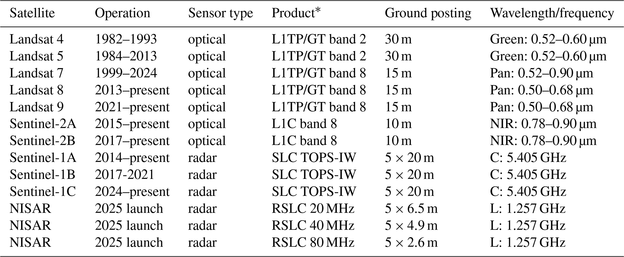
^* LITP = Level 1 precision and terrain correction. LIGT = Level 1 systematic terrain-corrected. SLC TOPS-IW = Single Look Complex Terrain Observation by Progressive Scan Interferometric Wide Swath. RSLC = Range Doppler Single Look Complex acquired at 20/40/80 MHz.

3.1.1 Optical data from Landsat 4–9 and Sentinel-2A/B/C

ITS_LIVE continuously processes optical images from Landsat 4 (1982–1993), Landsat 5 (1984–2013), Landsat 7 (1999–2024), Landsat 8 (2013–present), Landsat 9 (2021–present), Sentinel-2A (2015–present), Sentinel-2B (2017–2025), and Sentinel-2C (2024–present); see Table 1. Surface displacements are calculated for “same-path-row” image pairs that are acquired from the same satellite position and look geometry and are separated in time by fewer than 546 d. To increase data density prior to the launch of Landsat 8, images acquired from differing satellite positions (i.e., cross-path row), generally from crossing ascending and descending orbits, are also processed if they have a time separation between 10 and 96 d. Feature tracking of cross-path-row image pairs produces velocity fields with lower signal-to-noise ratio due to residual parallax from imperfect terrain correction that is largely self-canceling in imagery acquired with the same viewing geometry (i.e., same-path row).

All optical images are pre-processed using a 5 × 5 Wallis operator to normalize for local variability in image radiance caused by shadows, topography, and sun angle, all of which can generate spurious artifacts when applying feature tracking to derive surface flow from optical imagery. For Landsat 4 and 5 band 2 images, along-track artifacts introduced by the Thematic Mapper whisk-broom sensor are removed using Fourier filtering. Missing data in Landsat 7 images, introduced after the scan line corrector failure in May of 2003, are filled with random noise so that they do not contribute to the amplitude of the correlation peak used in the feature tracking.

Using autoRIFT, pre-processed same-path-row and cross-path-row pairs of images are searched for matching features by finding local normalized cross-correlation (NCC) maxima at sub-pixel resolution by oversampling the correlation surface by a factor of 16 using a Gaussian kernel. As a first step, a sparse grid pixel-integer NCC search ($\mathrm{1}/\mathrm{16}$ of the density of the full search grid) is used to determine areas of coherent correlation between image pairs. Results from the sparse search guide a dense search with search centers spaced such that there is 50 % overlap between adjacent template windows. Areas of unsuccessful retrievals, as determined using a normalized displacement coherence (NDC) filter (Gardner et al., 2018), are searched with progressively increasing template chip sizes. Minimum and maximum acceptable template chip sizes for each search center are defined geographically and depend on land surface type (ice or rock), spatial gradient of a reference velocity mapping, distance from the ocean, and distance from the ice edge. The data are then filtered one last time using the NDC filter, and small data gaps are filled by interpolation. Interpolated values are indicated in each image pair data product as interp_mask = 1. Our reference velocity is derived from a synthesis of version 1 MEaSUREs ITS_LIVE Regional Glacier and Ice Sheet Surface Velocities (Gardner et al., 2022), MEaSUREs version 1 of the Multi-year Greenland Ice Sheet Velocity Mosaic (Joughin et al., 2016), and version 1 MEaSUREs Phase-Based Antarctica Ice Velocity Map (Mouginot et al., 2019).

To reduce computational demand, autoRIFT employs a downstream search that centers the NCC search template window in the search image at the expected downstream location of displacement, as determined from the reference velocity. The NCC search radius is unique in both x and y directions and varies spatially. The NCC search radius is defined according to the surface type (ice or rock), magnitude of the component reference velocity (vx, vy), and distance from the ocean. Ocean area is identified according to the Global Self-consistent, Hierarchical, High-resolution Geography Database (GSHHG). In Greenland, land ice area is identified according to a dataset provided by Frank Paul (Bolch et al., 2013); in Antarctica, land ice is identified according to Depoorter et al. (2013), and everywhere else land ice is determined using the Randolph Glacier Inventory Release 6.0. Rock is defined as neither ocean nor land ice.

3.1.2 SAR data from Sentinel-1A–1B

The ITS_LIVE project also includes velocity products derived from synthetic aperture radar (SAR) imagery. SAR imagery has qualities that are valuable for imaging of polar glaciers and ice sheets as retrievals are not obscured by cloud or limited by solar illumination. These capabilities are highly complementary to optical retrievals. ITS_LIVE continuously processes “same-path-frame” SAR images from Sentinel-1A (2014–present), Sentinel-1B (2016–2021), and Sentinel-1C (2024–present) (see Table 1), separated by 12 d or fewer. When applied to SAR imagery, autoRIFT generates a rotation matrix that allows derivative surface velocities to be generated from two Level 2 ITS_LIVE granules, one ascending and one descending, using only range offsets that are significantly more precise than azimuth offsets (Joughin et al., 1998).

Processing of SAR data closely mimics the processing steps described for optical data, with the following distinctions: all Sentinel-1 Single Look Complex (SLC, Level 1.1) of TOPS IW mode data are pre-processed using the NASA/JPL InSAR Scientific Computing Environment version 2 (ISCE2) software (https://github.com/isce-framework/isce2, last access: February 2025) prior to dense offset tracking, where the two SLC images are precisely co-registered using the satellite orbit geometry. We use the Global Copernicus GLO-30 digital elevation model in our SAR processing. All SAR images are pre-processed using a 21 × 21 Wallis operator to normalize for local variability in radar backscatter caused by topography, followed by a 32 bit floating point to 8 bit integer data compression to save space and improve efficiency. Pre-processed same-path-frame pairs of images are searched for matching features by finding local normalized cross-correlation (NCC) maxima at sub-pixel resolution by oversampling the correlation surface by a search-chip-size-dependent factor. Correlation surface oversampling values of 32, 64, 128, and 128 are used for chip sizes of 240, 480, 960, and 1920 m, respectively, using a Gaussian kernel (Lei et al., 2022). The search-chip-size-dependent factor is used to match the oversampling ratio with maximum achievable precision from the data. See Lei et al. (2022) for a more detailed description of the Sentinel-1 processing.

3.1.3 Velocity uncertainty in Level 2 image pairs

Sources of uncertainty in ITS_LIVE Level 2 velocity data products are related to the accuracy of the geolocation that can be obtained for an image pair and the quality of the correlation peak for a given sub-image pixel match. The observed initial offset error, assessed as the uncorrected offset to stable surfaces (rock or slow-moving ice), averages under half a pixel for both Landsat 8 and Sentinel-2A/B/C and less for Sentinel-1A/B/C, but it can be as large as a full pixel. Geolocation offsets are corrected by adjusting scene pair velocities to known stable surfaces such as rock or slow-moving ice, and after correction, displacement accuracy is better than a tenth of a pixel (Lei et al., 2021). Correlation-related errors are also on the order of less than a pixel where correlation peaks are distinct. With restrictive masking of weakly correlated offset matches, remaining offsets over stationary targets have conservative root mean square errors of 0.1 pixels, which translate to conservative estimates of individual velocity errors of ∼ 1 m d⁻¹ for a pair of Landsat images separated by 16 d, or 0.12 m d⁻¹ error for a pair of Landsat images separated by 96 d, in agreement with similar data products (Mouginot et al., 2017). Offset errors are significantly smaller with larger search chip sizes, and, as each search chip used for offset determination contains 50 % overlap with adjacent chips, the surrounding offsets can be averaged with the error decreasing as

$$\mathit{v}x/y\mathit{\_}error\cong {\displaystyle \frac{\mathrm{mean}(vx/y\mathit{\_}error)}{{\left(\frac{n}{\mathrm{4}}\right)}^{\mathrm{2}}}},$$

where n is the number of offsets averaged. To correct for geolocation errors, component velocities vx and vy are tied to a “stable” surface wherein the median of each velocity component is set to zero over rock surfaces and set to the median reference velocity over slow-moving areas (ice movement of less than 15 m yr⁻¹) of Greenland and Antarctica. If an image pair does not intersect a stable surface, an alternative error metric is included with almost equivalent performance that uses the area of the slowest 25 % of the reference velocity. After geolocation corrections are applied, velocity uncertainty in each component direction is calculated as the root mean square of measured velocities over the stable reference surface. An additional error metric v_error is calculated as

$$v\mathit{\_}error=\sqrt{{\left(vx\mathit{\_}error\times {\displaystyle \frac{vx}{v}}\right)}^{\mathrm{2}}+{\left(vy\mathit{\_}error\times {\displaystyle \frac{vy}{v}}\right)}^{\mathrm{2}}}.$$

SAR orbit and viewing geometry between same-path-frame image pairs are highly stable, so the geolocation error is very small for an image pair consisting of the same satellite (both images from Sentinel-1A or both from Sentinel-1B). However, the inter-satellite (Sentinel-1A/B) image pairs suffer from subswath-dependent and full-swath-dependent geolocation errors due to systematic issues. To correct for subswath-dependent geolocation error, 11 Sentinel-1A/B image pairs were characterized over the interior of Greenland with slow-moving ice surface, and the inter-swath range/azimuth pixel offset bias estimates are then used as a static correction of the subswath-dependent geolocation error in each ITS_LIVE Sentinel-1 image pair product (Lei et al., 2022).

3.2 Data cubes

After generating Level 2 image pair data, a cloud-optimized data cube product is generated internally to collect Level 2 data for compositing and mosaicking. In this process, each glacierized region is subdivided into 100 km by 100 km tiles, and Level 2 data within each tile are stored as layers in a Zarr data format.

3.3 Level 3 composites and mosaics

Individual annual and climatological composites are created for each 100 km by 100 km data cube. As a first step, Level 2 optical and SAR data undergo numerous quality controls to account for issues related to geolocation errors, sensor-specific performance, and feature locking, all of which are described in Appendix A. Filtered Level 2 optical and SAR image pair velocities are combined to form annual composites for the data cube using an error-weighted least-squares approach that simultaneously solves for the mean annual velocity and a sinusoid that characterizes the climatological average seasonal cycle (Greene et al., 2020). In this approach, total displacement measured between the acquisition times of each image pair is fit to an amplitude and phase of a sinusoid and a constant value corresponding to each year. Displacement coefficients are then converted to velocity values to obtain annual mean velocity values vx, vy, and v. The result is a mathematical best-fit characterization of typical seasonal velocity variability that accounts for total displacement over long polar winters when optical data are often unavailable and an annual mean velocity value that is unbiased by the timing of image acquisitions throughout the year. In this process, outlier observations determined by a median absolute deviation filter are discarded after an initial fit to all data, and then the fit is repeated with outliers removed.

In addition to annual velocity values, overall summary climatology composites are generated for each region as Level 3 data files containing 0000 in place of a year in the filename. Summary velocities are calculated using a least-squares fit applied to image pair data with a mid-date between 1 January 2014 and 1 January 2023. Seasonal components (vx_amp, vy_amp, v_amp, vx_phase, vy_phase, v_phase) are determined directly from the least-squares fit. The mean velocity and velocity trend are determined from an error-weighted linear fit to the annual values. We then solve the fit velocity for an arbitrary date of 2 July 2018 to create a consistent map of velocity with minimal spatial variation that might otherwise be caused by a simple mean of the data available in each grid cell. The intention here is to create a best snapshot of flow that can be used in mass-conserving divergence or gradient calculations, with a consistent effective timestamp across all pixels. The slope of the linear fit to annual values is also provided as velocity trends dvx_dt, dvy_dt, and dv_dt in the summary mosaic file. Note that the date range used for climatology calculations will be updated as the record lengthens. It is recommended that users inspect product metadata to confirm the dates of the input data.

Regional mosaics are then created by re-projecting 100 km by 100 km composites into a common projection and merging. When re-projecting those data, care is taken to rotate and scale the velocity components to be consistent with the target map projection. Overlapping composites are weighted by data counts. Count is taken as the maximum count of overlapping composites. ITS_LIVE produces mosaics for the 16 regions shown in Fig. 2 that cover the majority of glacierized area. For areas that fall outside of these 16 regions, users can work directly with the unmerged composites.

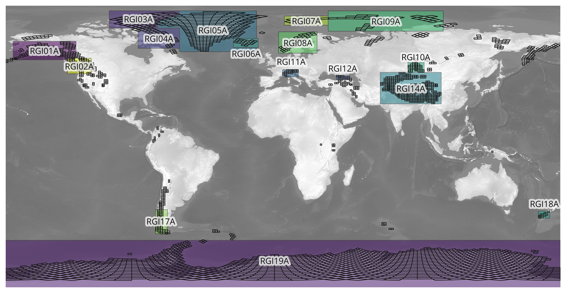
Figure 2 Shaded rectangles show the coverage of the 16 ITS_LIVE mosaic regions. Regions follow a similar naming convention as the Randolph Glacier Inventory version 6. All 3086 100 km by 100 km ITS_LIVE data cubes are shown with black outlines.

3.3.1 Error estimates and quality metrics

Annual velocity mosaics contain a count variable indicating the number of image pairs that at least partially contribute to the error-weighted least-squares fit for that year. Annual mosaics also contain estimates of vx_error, vy_error, and v_error, which are error-weighted means of error estimates of all contributing Level 2 data for each year.

Climatology mosaics containing 0000 in the filenames include a count variable indicating the total number of image pairs used to estimate the climatology velocities, trends, and seasonal variability and an outlier_percent indicating the percentage of Level 2 data excluded from the Level 3 climatology fit. Formal errors from Level 2 products are propagated through to the annual mosaics but can produce an overly optimistic estimate of product errors, so we adopt a more conservative approach and calculate the errors as the standard error of the mean. This is calculated by taking the root sum of squares of the residuals to the least-squares fit and dividing by the number of observations. Annual errors are then propagated to determine mean flow mosaics errors. Estimates of vx_amp_error, vy_amp_error, and v_amp_error describe the overall mismatch of velocity observations to the seasonal fit. Uncertainty of seasonal phase values cannot be estimated formally but is expected to be accurate within a few days or weeks where amplitudes are significant and hundreds of image pairs or more contribute to the fit (Greene et al., 2020).

4 Data counts and global statistics

ITS_LIVE version 2.0 global velocity mosaics describe the flow of 14 190 690 km² of Earth's land ice, covering every glacier larger than 5 km² north of 83° S. The data reveal diverse landscapes of glacier flow and complex responses to an evolving climate. The summary mosaics show that the world's fastest land ice is in Greenland, where the central trunk of Sermeq Kujalleq (Jakobshavn Glacier) exceeds 10,000 m yr⁻¹. The fastest grounded ice in Antarctica flows from Pine Island Glacier into the Amundsen Sea at more than 4000 m yr⁻¹, and the fastest glacier outside the great ice sheets is Hubbard Glacier in Alaska, where average speeds exceed 3000 m yr⁻¹. Annual mosaics show that Alaska's Columbia Glacier exhibits velocities comparable to Hubbard Glacier near its terminus, but its top speed is not accurately reflected in the climatology due to rapid retreat that has been ongoing there since the 1980s. Elsewhere in the Arctic, Storisstraumen Glacier (Basin 3) in Svalbard has averaged nearly 3000 m yr⁻¹ while slowing steadily at a rate of 200 m yr⁻² over the past decade. Glaciers in middle to low latitudes are generally characterized by slow velocities. However, areas of fast flow are observed for the largest glaciers (e.g., Pio XI glacier in the Patagonian ice field reaches 3000 m yr⁻¹, and Fedchenko glacier, Pamir, reaches 800 m yr⁻¹), at localized icefalls (Khumbu icefall, Nepal, up to 400 m yr⁻¹; Bossons icefall, French Alps, up to 500 m yr⁻¹) or during glacier surges, which are particularly prevalent in Pamir and Karakoram (Khurdopin glacier, Karakoram, peaked above 3500 m yr⁻¹ in May 2017).

Level 3 summary mosaics of ITS_LIVE version 2.0 confirm that glaciers around Greenland have accelerated over the past decade, and Antarctica's most significant dynamic changes are concentrated in the Amundsen Sea Embayment, most notably at Pine Island and Thwaites glaciers. Although velocity variability is seen in every region of the globe, glaciers have not responded uniformly to recent climate change. In the data, we do not see any definitive global bias toward glacier acceleration or deceleration since 2014, but we do see subtle regional trends and a diversity of behaviors within each region. The largest magnitudes of dv_dt in Alaska are driven by surges, and the signs of these linear trends are closely linked to the timing of surge activity. For example, the velocities of Seward, Steller, and Lowell glaciers all trended upward in the past decade due to recent surge events, while the velocities of Fisher, Walsh, and Klutan trended downward following surge events that initiated in 2015 and 2016. Similarly, several glaciers in Svalbard and the Canadian Arctic show decadal velocity trends that can be attributed to timing of surge events.

Globally, the highest concentration of high-amplitude seasonal variability is observed in Alaska, where velocities tend to peak in spring or summer. In contrast, some glacier velocities in High Mountain Asia peak in spring, while others peak in fall. We confirm previous reports of seasonally variable discharge in Greenland that peaks in summer (King et al., 2018) but find little evidence of seasonal variability around Antarctica, particularly on grounded ice.

In total, more than 36 000 000 image pairs currently contribute to ITS_LIVE version 2.0, beginning with the 1982 launch of Landsat 4. The record is somewhat sparse globally until the 2013 launch of Landsat 8 (Fig. 3), which was followed by yearly launches of Sentinel satellites through 2017 and the launch of Landsat 9 in 2021. Now, almost every grid cell in the world is captured by multiple satellites each year, velocity is directly measured throughout long polar nights with the Sentinel-1 satellites, and some locations are characterized by as many as 100 000 velocity estimates per year. The sheer volume of observations now available suggests that glaciology is no longer a field held back by data starvation.

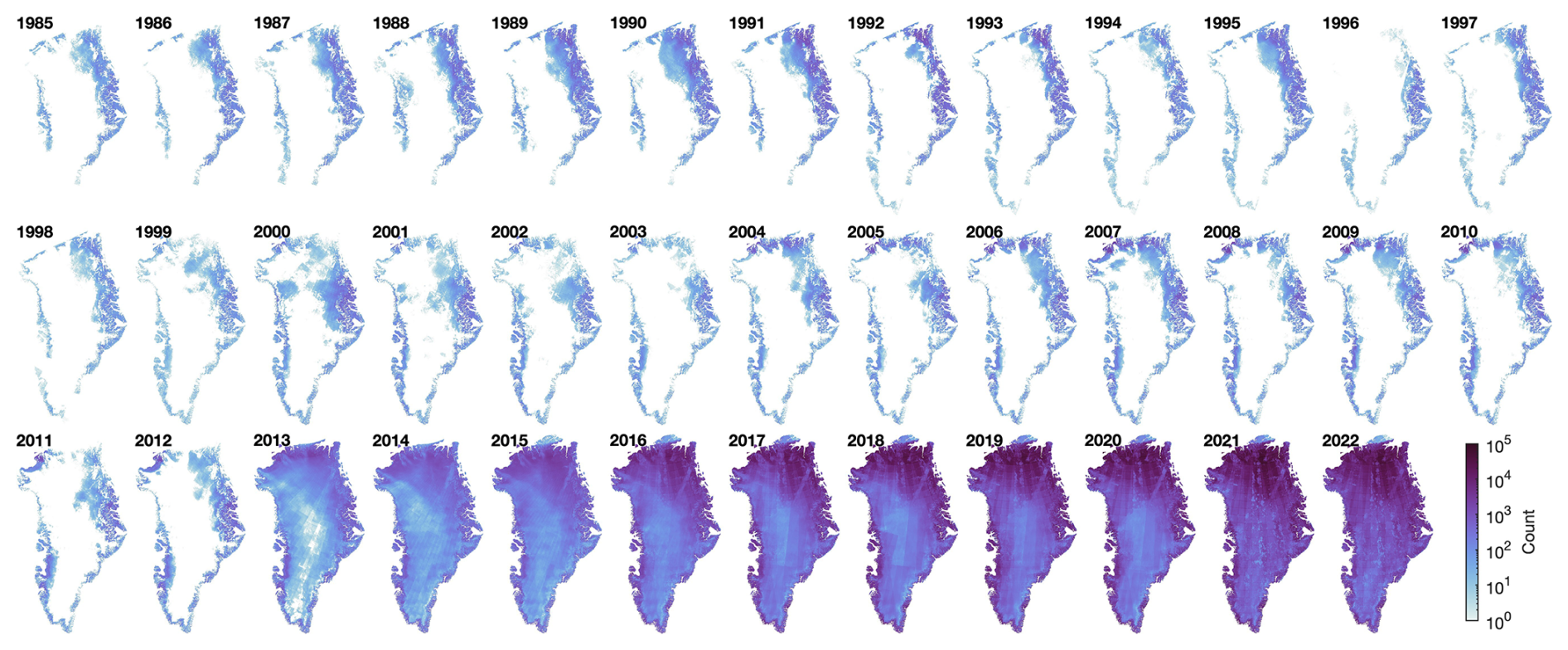
Figure 3 Time series of the number of Level 2 image pairs contributing to each grid cell of each Level 3 annual velocity mosaic of Greenland. Satellite names appear in the first year they contribute to an annual mosaic in ITS_LIVE version 2.0.

4.1 Limitations and uncertainties

Although Level 2 image pairs can be processed within minutes of satellite image availability, some appreciable lag is necessary before Level 3 mosaics can be generated. Because we process image pairs separated by up to 546 d, some observations covering December 2023, for example, will not be available until their paired images are acquired in June 2025. To ensure that all available data are included in annual mosaics, ITS_LIVE generates Level 3 mosaics in dedicated campaigns after all contributing images are acquired.

Level 2 image pairs are most accurate where rock or other stable surfaces are present within the satellite image frame for georeferencing. Data users should be aware that feature tracking directly measures displacements, and precision is limited by image pixel size and image quality. Velocity is calculated as displacement over time, so errors in velocity can be mitigated by increasing the time between images (dt), but long separation times between images come at the cost of temporal resolution and can allow the surface to change or lose its distinguishing features between image acquisitions. As described above, at some locations near ice edges, ice falls, or bends in glacier flow, surface patterns may be replicated with enough similarity that long values of dt confuse the feature tracking algorithm by allowing it to skip or lock onto the incorrect pattern cycle. A filter is in place to identify and discard velocity values that likely correspond to skipping or locking before Level 3 mosaics are calculated (Sect. 3.3 and Appendix A), but users of Level 2 data should be aware of the potential benefits and risks of using image pairs with short versus long dt values.

Level 3 velocity uncertainty is reduced where an abundance of Level 2 observations are available, so mosaics generally have lower uncertainty values toward the poles, where satellite orbit patterns converge and many images overlap. Low data counts can result from sparse orbits, persistent cloud cover that obscures optical images, or high accumulation rates that create featureless or frequently changing surfaces that cannot be tracked. For example, data counts are particularly low along the high peaks of the southern Andes, where cloud cover is common and accumulation rates are high. Whereas the median data count among land ice grid cells is 5407 in the summary mosaic of Region 5 (Greenland), the median value is only 881 in Region 17 (South America), and some high-elevation locations in this region have nearly no valid data at all.

Metrics of seasonal variability are most accurate where several hundred or more image pairs contribute to the sinusoid fit (Greene et al., 2020). This condition is met in most locations around the world, but where data counts are lower, the least-squares fit becomes especially sensitive to extreme velocity values and v_amp may be larger than the true amplitude of seasonal variability. We note that the sinusoid fit to the seasonal cycle is a best-fit model that describes only the fundamental mode of seasonal variability and does not account for higher-order acceleration/deceleration or changes in seasonal behavior from one year to the next. The timing of the maximum velocity in a sinusoid fit may not align with ephemeral spikes in velocity, and although filters are in place to remove outliers before performing the final fit, discrete events such as glacier surges can in some cases contaminate the overall seasonal characterization. We recommend exploring the complete time series of Level 2 data at any given location to interpret the summary mosaic metrics of seasonal variability. Similarly, interpretation of dv_dt velocity trends since 2014 may warrant inspection of the complete time series to determine any potential influence of surge-type behavior that is nonlinear by nature and cannot be accurately characterized by a linear fit.

The update of ITS_LIVE velocity data from version 1.0 to version 2.0 includes a change in reporting of velocity values. Whereas version 1.0 included a correction for map distortion, velocities in version 2.0 are now reported in map units of the projection in which the data are published. Projection distortion can be on the order of a few percent in some locations and should be corrected when comparing to in situ observations (e.g., GPS), but the change was made for consistency within the data product, to allow calculation of flow lines from the velocity components in map projected coordinates, and to allow flux estimates that no longer require the flux gate cross-section to be corrected for map distortion.

5 Data access and tools

ITS_LIVE version 2.0 velocity data are hosted on AWS as part of the AWS Open Data Sponsorship Program and served through NASA's National Snow and Ice Data Center Distributed Active Archive Center (NSIDC DAAC). The data can be accessed in several ways according to user needs and preferences.

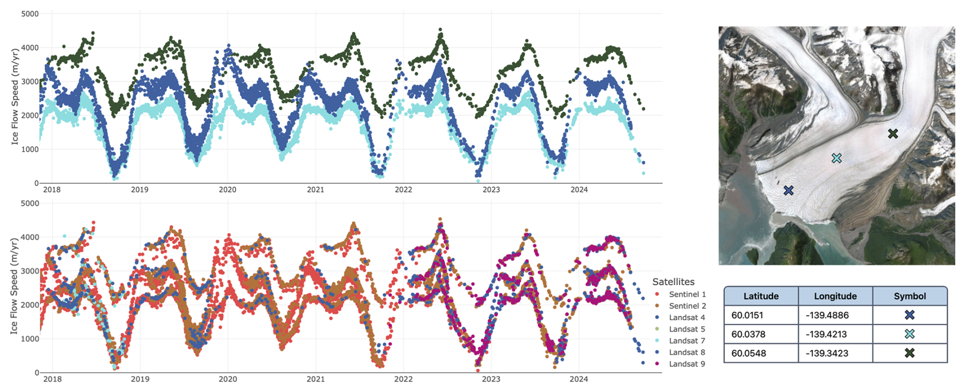
Figure 4 An example velocity record for lower Hubbard Glacier, Alaska. Upper left: ice flow speed for three points shown on the map on the right. Lower left: The same data, color-coded by satellite. Sentinel-1 (red) adds significant detail and sampling density in this very cloudy coastal setting and provides speeds through the winter. Basemap from Earthstar Geographics (TerraColor NextGen) imagery. An interactive version of this figure can be accessed at https://its-live.jpl.nasa.gov/app/index.html?z=11&lat=60.0151&lon=-139.4886&lat=60.0378&lon=-139.4213&lat=60.0548&lon=-139.3423&int=1&int=100&x=2017-11-10&x=2024-12-12&y=-31&y=5115, (last access: February 2025).

Level 2 image pairs and Level 3 mosaics can be accessed through the NSIDC using the ITS_LIVE app at https://nsidc.org/apps/itslive/ (last access: February 2025​​​​​​​). In this app, users can pan and zoom an interactive map to find Level 3 annual and summary mosaics for each region or build search queries to find and download Level 2 image pair granules as NetCDF files. A suite of other Python tools and notebooks are available at https://github.com/nasa-jpl/its_live (last access: February 2025​​​​​​​), and similar utilities for data download and analysis are available for Julia and MATLAB users, links to which are provided on the main ITS_LIVE website (https://its-live.jpl.nasa.gov, last access: February 2025) along with other helpful information.

The Level 2 velocity pipeline generates a large amount of data such that any single point on Earth may be covered by 100 000 image pairs or more. To eliminate the need for users to download or open such a large number of granules, ITS_LIVE also provides all Level 2 data in 3086 100 km by 100 km cloud-optimized Zarr data cubes that are structured for rapid time series access. The data cubes retain all fields and metadata from the original Level 2 data and are hosted on public AWS S3 cloud storage, allowing users to write generic workflows that do not require downloading tens or hundreds of thousands of individual Level 2 NetCDF files. ITS_LIVE also hosts a geojson catalog of all of the data cubes on public S3 cloud storage. Utilities for working with Zarr data cubes can be found at https://github.com/nasa-jpl/its_live.

The adoption of cloud-hosted, cloud-optimized Zarr data cubes has enabled the creation of a serverless web app (Fig. 4) that allows users to interactively explore glacier velocity time series at any location on Earth. The interface allows users to enter geographic coordinates or select points on a map to instantly plot the full record of velocity data at specified locations. Users can then share a hyperlink to the same map with collaborators or students for frictionless workflows and lesson plans that are open and replicable. The map interface can be accessed at https://its-live.jpl.nasa.gov/app/index.html(last access: February 2025​​​​​​​).

6 Conclusions

One of ITS_LIVE's goals is to provide as complete a record of ice flow as practical from online imagery collections – an observational record of glacier flow that is global in scope, processed with open-source tools in a consistent way, and that can be extended with new data as they are acquired. ITS_LIVE has now processed more than 36 million satellite image pairs, spanning the globe and covering four decades and counting. The data are free and easily available in multiple file formats and can be accessed locally or in the cloud, and open-source tools are available in multiple computing languages to help users access, analyze, and understand the data. The release of version 2.0 preserves traditional NetCDF granule access while also supporting cloud-native Zarr access for modern big-data machine learning applications. Level 2 image pairs are available for process studies that require high-resolution reconstructions of dynamic time series; Level 3 mosaics can easily be employed to estimate ice sheet mass discharge and sea level contributions; and together, the ITS_LIVE products will enable precise ice sheet and glacier model calibration and validation for improved projections of future changes in Earth's climate system. Version 2.0 velocity products complement additional ITS_LIVE geophysical data products of surface elevation (Nilsson et al., 2022, 2023; Nilsson and Gardner, 2024), ice shelf basal melt (Paolo et al., 2024, 2023), and ice sheet extent (Greene, 2024; Greene et al., 2022, 2024), which together aim to characterize changes in the world's ice in every dimension, in usable, interoperable formats.

Version 2.0 of ITS_LIVE velocity products have been processed at 120 m resolution globally, which is an improvement over the 240 m resolution of the version 1.0 products. Future releases of ITS_LIVE velocity data products are expected to include data from the Sentinel-1C and NISAR. ITS_LIVE is also assessing ways to fill in the historical archive with data from the Advanced Spaceborne Thermal Emission and Reflection Radiometer (ASTER) instrument that was launched aboard the Terra satellite in 1999 and RADARSAT-1 that was launched in 1995 and decommissioned in 2013.

The dense spatiotemporal coverage of the ITS_LIVE version 2.0 and future releases will help scientists discover previously unknown patterns of glacier flow and the mechanisms that cause and control them. In the data, users will find glaciers surging, shear margins migrating, kinematic waves propagating up and down glaciers, dynamic responses to calving events and ice shelf thinning, and speedups and slowdowns driven by seasonal changes in basal hydrology. A world of new insights now resides in ITS_LIVE version 2.0 and is waiting to be discovered.

Appendix A

The following details the processing steps used to generate composites from the multi-sensor data cubes (one composite per data cube).

• A.

  Add systematic errors to image pair component velocity errors based on the level of co-registration as indicated by the “stable_shift_flag” attribute that is included with the product. The stable_shift_flag is a flag for tracking the velocity bias correction: 0 = no correction; 1 = correction from overlapping stable surface mask (stationary or slow-flowing surfaces with velocity <15 m yr⁻¹) (top priority); 2 = correction from the slowest 25 % of overlapping velocities (second priority). A random error for each image pair is provided with each granule and is calculated as the standard deviation between the reference and the measured component velocities over the co-registration surface (i.e., stable or slowest 25 %). A default random error is assigned when stable_shift_flag = 0. We add an additional systematic error to the random errors as listed in Table A1.

• B.

  Over ice sheets it was found that image pairs that were co-registered to limited areas of “stable” surfaces could contain unrealistically small velocity errors. These unrealistically small errors cause issues with the error-weighted composite generation. To correct for this, in regions RGI05A (Greenland) and RGI19A (Antarctica), we replaced vx_error and vy_error with vx_error_slow and vy_error_slow, respectively.

• C.

  Apply a StableShiftFilter. This routine discards low-quality image pair data that have absolute $vx/vy\mathit{\_}stable\mathit{\_}shift$ values that exceed, per each mission group, the thresholds (thresholds determined from histograms of stable_shift values for each sensor) that are listed in Table A2.

  If an image pair exceeded the mission-specific threshold in StableShiftFilter (i.e., very large $vx/vy\mathit{\_}stable\mathit{\_}shift$ have been applied) then the following actions were taken: if $stable\mathit{\_}shift\mathit{\_}flag==\mathrm{1}$ then the image pair was excluded and if $stable\mathit{\_}shift\mathit{\_}flag==\mathrm{2}$ then the stable shift was removed from the velocity field (i.e., added back to $vx/vy/vr/va$).

• D.

  ITS_LIVE velocities are produced by finding correlated features between two image chips, a process referred to as feature tracking. In some locations, feature tracking can be susceptible to surface “skipping” or “locking”, where instead of tracking the surface features that are the intended targets, the correlation incorrectly locks onto features that have shapes that are similar to the intended target features (Fig. A1). The problem is caused by high-frequency radiometric features that are not removed by the high-pass filter and are stationary because of topography, surface water, curved flow lines (constrains both x and y), crevasse chains, or some combination of all. Radar speckle tracking will also suffer from “skipping” where high-frequency stationary features exist in the amplitude image (ice falls, curved flow lines, surface water). The degree of locking/skipping depends on the surface features, sensor characteristics (spatial resolution, radiometric resolution), high-pass pre-processing filter, and search chip size. The three places where skipping/locking is most prevalent are near ice edges, ice falls, and flow bends.

  Sensors that have a lower spatial and/or radiometric resolution and image pairs that are acquired further apart in time are most prone to surface skipping/locking. We apply the SensorExcludeFilter to identify and remove surface skipping/locking errors as follows.

  • a.

    Load the landice_2km_inbuffer mask for the data cube being processed. landice_2km_inbuffer is a binary mask that defines the extent of glacierized areas after applying a 2 km inward buffer from the glacier edge.

  • b.

    Define sensor groups: Landsat 4/5, Landsat 7, Landsat 8/9, Sentinel-2, Sentinel-1

  • c.

    Exclude any data that have a velocity magnitude >20 000 m per year from further analysis.

  • d.

    Apply SensorExcludeFilter for locations that are within 2 km of the ice edge: landice_2km_inbuffer mask $==$ 0. The following steps are taken when applying the SensorExcludeFilter.

    • i.

      Sentinel-2 image pair data are used as the reference sensor group as they are least prone to skipping/locking errors. If there are no Sentinel-2 granules for a given location then the SensorExcludeFilter is not applied.

    • ii.

      Only include image pair data with time separation less than or equal to 64 d. This is done as image pair data with longer time separations are more prone to skipping/locking errors.

    • iii.

      For each sensor group we compute mean vx and mean vy and then calculate the unit vector. All image pair vx and vy are then projected onto their corresponding sensor group unit vector.

    • iv.

      Projected velocities are binned into $\mathrm{1}/\mathrm{5}$ of a year bins spanning the time range of the Sentinel-2 data. For bins with more than three values the following statistics are calculated: mean projected velocity, standard deviation, and count. If the reference sensor (Sentinel-2) has no bins with more than three values then the SensorExcludeFilter is not applied.

    • v.

      For each non-reference sensor group we identify bins that are valid for both the sensor group and the reference sensor. If there are fewer than three co-valid bins then we do not apply the SensorExcludeFilter to that sensor group. If there are more than three co-valid bins we compute the standard error between the co-valid projected velocities. If the mean of the co-valid sensor group values is 3 times the standard error below the mean of the reference sensor, then the sensor group is excluded from composites calculation at that pixel location. Here, excluded values are likely experiencing significant skipping/locking errors and should therefore not be included in the composites.

• E.

  Next, we apply the MaxDtFilter that determines the maximum image pair time separation that should be included in the composite creation. This is done to minimize skipping/locking errors that are more prevalent with increasing image pair time separations. A maximum image pair time separation (dt_max) is determined for each sensor and each location as follows.

  • a.

    Calculate the median composite velocities for all image pair data with time separation less than or equal to 16 d. Each point must have at least 50 valid values. If a location has fewer than 50 valid values, the time separation threshold is progressively increased from 16 to 32 to 64 to 128 to 256 to infinity until at least 50 valid values are identified. If this condition is never met then the location is set to “no data” in the composite creation. Where the condition is met, we calculate the median velocity magnitude and unit flow vector from the median composite velocities.

  • b.

    If the median velocity magnitude is less than or equal to 50 m yr⁻¹ then MaxDtFilter is not applied.

  • c.

    Project all image pair velocities to the median unit flow vector.

  • d.

    Bin projected velocities by image pair time separation into bins with edges 0, 16, 32, 64, 128, 256, and infinity days.

  • e.

    For each bin calculate the median, count, and median absolute deviation from the median (MAD).

  • f.

    Compute minimum and maximum projected velocity bounds for each bin based on median ± MAD.

  • g.

    Identify a reference bin as the first bin with 50 or more velocities moving from bin 0 to 16 d through to 256 to infinity days. If no such bin exists, the reference bin is set to the first bin with two or more velocities. If no such bin exists, MaxDtFilter is not applied.

  • h.

    Find the first bin, moving from bin 0 to 16 d through to 256 to infinity days, that does not have overlapping bounds with the reference bin. Set the maximum allowed time separation (dt_max) equal to the lower bound of the identified bin. If all bins overlap then dt_max is set to infinity.

  • i.

    For composite creation, only include data for which the image pair time separation is less than or equal to dt_max.

• F.

  Determine annual and climatological glacier velocities for each 120 m pixel location following Greene et al. (2020).

  • a.

    Apply a 15-point moving window filter to all input velocity data.

  • b.

    Create a matrix M of coefficients that define the percentage of each year spanned by each image pair. The matrix M is used in the least-squares calculation to obtain a mean annual velocity corresponding to each year.

  • c.

    Calculate the least-squares weighting for each value as 1 divided by the square of the displacement error (velocity error time dt).

  • d.

    Determine annual composite outputs as the optimal fit of all valid data in an error-weighted least-squares sense.

  • e.

    For climatological composites we do the same least-squares fit but only include image pair data with a mid-date between 1 January 2014 and 1 January 2023. Mean velocity and velocity trend are determined from an error-weighted linear fit to the annual data (time intercept of 1 January 2018).

• G.

  In areas distant from the ice edge ($landice\mathit{\_}\mathrm{2}km\mathit{\_}inbuff==\mathrm{1}$) and with low radiometric contrast, Sentinel-2 image pair velocities can contain high noise due to image processing artifacts. These artifacts can introduce significant noise into the composite creation. To mitigate this, we apply an S2Filter as follows.

  • a.

    Recompute the annual and climatological composite outputs excluding all Sentinel-2 data.

  • b.

    If the original seasonal amplitude is twice as large as the recomputed seasonal amplitude, and the difference in the seasonal amplitudes is greater than 2 m per year, then exclude Sentinel-2 data, at this location, from the composites.

• H.

  If annual velocity magnitude is greater than 20 000 m yr⁻¹ then all data for that year are excluded. If the seasonal amplitude is greater than 10 000 m yr⁻¹ then all data for that point are excluded.

Table A1 Systematic error added to $v[x/y]\mathit{\_}error$ as a function of stable_shift_flag.

Table A2 Mission-specific StableShiftFilter thresholds.

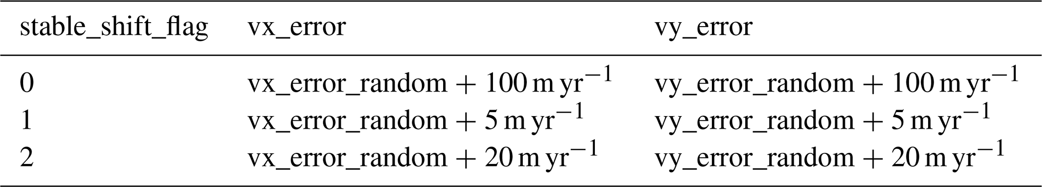
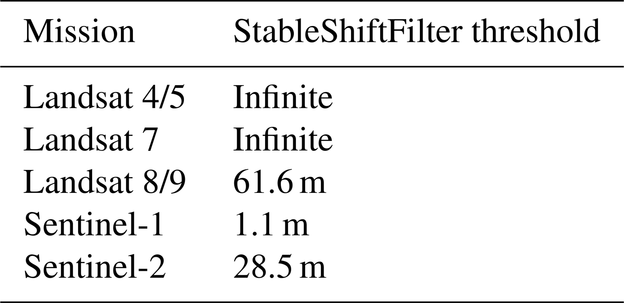
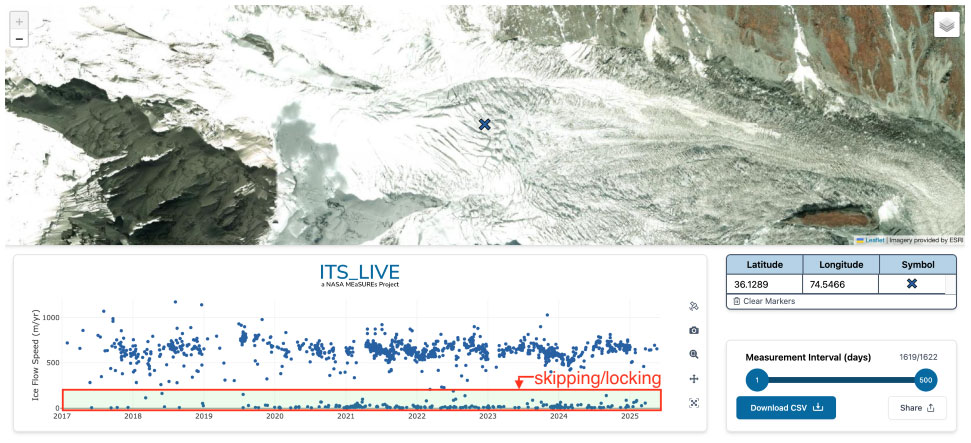
Figure A1 Example of surface skipping/locking feature tracking matches that result in periodic near-zero velocities. Retrieved flow speeds are shown for the blue “x” that is located at the edge of an ice fall. Flow speeds are generally in the range 300–1000 m yr⁻¹. The clustering of flow speeds near 0 m yr⁻¹ is erroneous and results from surface skipping/locking. Basemap from Maxar (Vivid) imagery captured on 15 October 2022. Image generated from ITS_LIVE app for data cube exploration: https://its-live.jpl.nasa.gov/app/index.html?z=15&lat=36.1289&lon=74.5466&int=1&int=500&x=2016-12-23&x=2025-06-08&y=-33&y=1202 (last access: August 2025​​​​​​​).