Brief communication: Representation of heat conduction into ice in marine ice shelf melt modelling

Basal melt of marine-terminating glaciers is a key uncertainty in predicting the future climate and the evolution of the Antarctic and Greenland ice sheets. Regional ocean circulation models rely on an approximated heat budget at the ice–ocean interface that includes turbulent heat flux from the ocean below, latent heat for phase transition, and heat conduction into the ice in order to parameterize melt rates. Here we review the formulations of Holland and Jenkins (1999) for the approximation of heat conduction into ice, utilizing three distinct observed ice temperature profiles. We show that the formulation accounting for constant vertical advection and vertical diffusion of heat into ice best represents the observed ice temperature profiles. Using idealized ocean simulations of a Greenlandic fjord and observed melt rates from Antarctica, we find a difference of up to 28 % (average of 12 %) in melt rates between the different approximations.

1 Introduction

In ocean general circulation models (OGCMs), marine-terminating glaciers are usually assumed to be static and the local melt rate is parameterized using a set of three equations consisting of a linearization of the local freezing point temperature of water as well as heat and salt budgets at the ice–ocean interface (Holland and Jenkins, 1999). The turbulent transport of heat from water to the ice–ocean interface is partly balanced by the heat conduction into the ice. Any excess heat from the combination of these two processes is used as latent heat for the solid-to-liquid phase change. Hence, a good representation of ice shelf basal melting in ocean models requires accurate simulations of both the turbulent heat transport in the water below the ice and the heat conduction into the ice shelf.

Heat conduction into ice has often been neglected in ocean simulations resolving ice shelf cavities, with the idea that the resulting bias does not affect melt rates by more than 10 % (Dinniman et al., 2016; Holland and Jenkins, 1999). Other models have adopted a crude representation of this flux by assuming a linear temperature profile between the freezing temperature at the ice shelf base and a typical annual mean air temperature at the ice shelf surface (e.g. Losch, 2008; Mathiot et al., 2017). More than 60 years ago, Wexler (1960) proposed a more elaborate formulation of this conductive heat flux by accounting for heat advection by vertical ice motion, based on the observation of a few vertical temperature profiles. The formulation was completed by Holland and Jenkins (1999), who proposed a linear approximation of Wexler's solution so that it can be incorporated into the solution of the three-equation system used to estimate basal melt rates in ocean models.

In this brief communication, we review these approaches and assess them using, for the first time, ice temperature profiles representing multiple typical scenarios of refreezing and melting. We further discuss the approaches' accuracies by applying them to realistic applications and estimate the influence of heat conduction on ice shelf basal melt rates around Antarctica. Additionally, we investigate the relative importance of the heat conduction in the presence of a realistic ocean circulation and possible ice–ocean feedbacks. We propose future directions to improve the calculation of these fluxes in ocean or Earth system models.

2 Assessment of the various approaches

The heat budget at the ice–ocean interface that is used to derive melt rates in ocean models can be expressed as

$$\begin{array}{}\text{(1)}& {\displaystyle }{\displaystyle }mL={\mathit{\rho }}_{\mathrm{w}}{c}_{\mathrm{w}}{u}_{\star }{\mathrm{\Gamma }}_{\mathrm{T}}\left(T_{\mathrm{w}}-T_{z_{\mathrm{d}}}\right)+{\mathit{\rho }}_{\mathrm{i}}{c}_{\mathrm{i}}{\mathit{\kappa }}_{\mathrm{i}}{\left({\displaystyle \frac{\partial T_{\mathrm{i}}}{\partial z}}\right)}_{z_{\mathrm{d}}},\end{array}$$

where m is the melt rate ($\mathrm{kg}{\mathrm{m}}^{-\mathrm{2}}{\mathrm{s}}^{-\mathrm{1}}$) (negative in the case of refreezing), ρ_w and ρ_i the densities of seawater and ice, L the melting or freezing latent heat of water, c_w and c_i the heat capacity of seawater and ice, u_⋆ the friction velocity calculated by the ocean model, Γ_T the turbulent transfer parameter of temperature, κ_i the heat diffusivity of ice, T_i the ice temperature, T_w the ocean temperature at some distance from the ice–ocean interface, $T_{z_{\mathrm{d}}}$ the local freezing point temperature, and z_d the ice draft vertical position (z negative below sea level and increasing upward).

The three common approximations made in ocean models to deal with heat conduction in ice are

$$\begin{array}{}\text{(2)}& {\displaystyle }{\displaystyle }\left\{\begin{array}{ll}{\mathit{\rho }}_{\mathrm{i}}{\mathit{\kappa }}_{\mathrm{i}}{\left(\frac{\partial T_{\mathrm{i}}}{\partial z}\right)}_{z_{\mathrm{d}}}=\mathrm{0}& \text{(A)},\\ & \\ {\mathit{\rho }}_{\mathrm{i}}{\mathit{\kappa }}_{\mathrm{i}}{\left(\frac{\partial T_{\mathrm{i}}}{\partial z}\right)}_{z_{\mathrm{d}}}={\mathit{\rho }}_{\mathrm{i}}{\mathit{\kappa }}_{\mathrm{i}}\frac{T_{\mathrm{s}}-T_{z_{\mathrm{d}}}}{z_{\mathrm{s}}-z_{\mathrm{d}}}& \text{(B)},\\ & \\ {\mathit{\rho }}_{\mathrm{i}}{\mathit{\kappa }}_{\mathrm{i}}{\left(\frac{\partial T_{\mathrm{i}}}{\partial z}\right)}_{z_{\mathrm{d}}}=\left(T_{\mathrm{s}}-T_{z_{\mathrm{d}}}\right)\text{max}\mathit{\{}m,\mathrm{0}\mathit{\}}& \text{(C)},\end{array}\right.\end{array}$$

where T_s is the ice surface temperature at height z_s.

Approximation (A) in Eq. (2) would be a good approximation if there were ice shelves close to the ocean freezing point over their entire thickness, but such ice shelves are likely unstable (Morris and Vaughan, 2003). It can still be a reasonable approximation for locations where ice shelves have a layer of marine ice at their base (Fig. 1a), although the permeable nature of this type of ice makes proper calculations complicated (Wang et al., 2022).

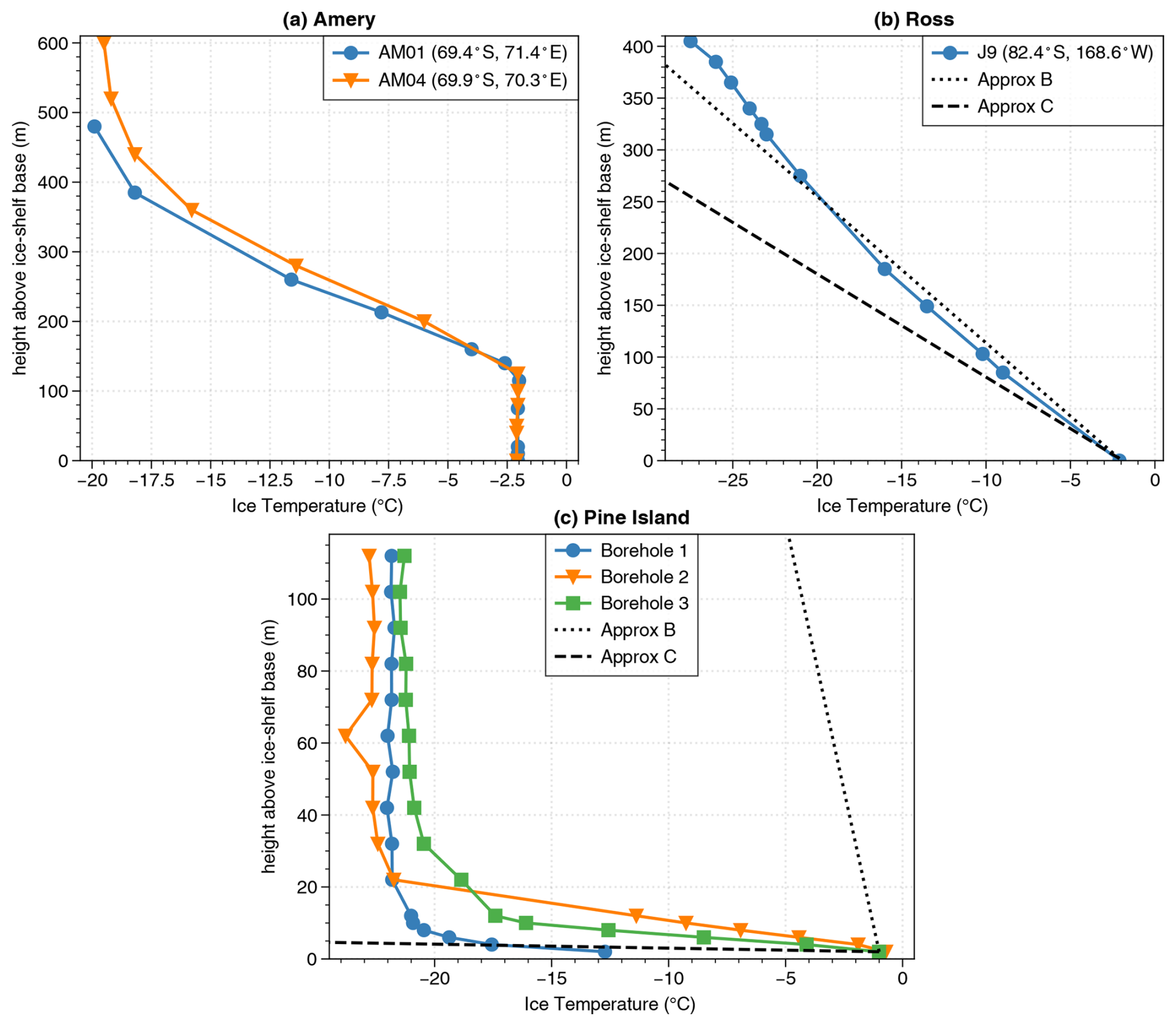
Figure 1 Ice temperature profiles measured by thermistor strings in boreholes at (a) two sites on the Amery Ice Shelf (69.4° S, 71.4° E and 69.9° S, 70.3° E, referred to as AM01 and AM04, respectively), (b) one site in the middle of the Ross Ice Shelf (82.4° S, 168.6° W, referred to as J9), and (c) three sites on Pine Island Ice Shelf (75.1° S, 100.5° W). The black dotted and dashed lines in panels (b) and (c) show temperature profiles approximated from Eqs. (2B) and (2C) using observed melt rates and the annually averaged surface temperature. A layer of marine ice is present underneath the ice shelf at sites AM01 and AM04 (more than 100 m thick) and at site J9 (6 m thick).

Approximation (B) in Eq. (2) assumes no heat advected by the ice and a temperature profile that has reached a steady state between the freezing temperature at the base and a constant surface temperature. This seems to be a good approximation for the Ross Ice Shelf (RIS, Fig. 1b). The ice typically takes 1000 years to go from the grounding line to the borehole of the shown temperature profile (Mouginot et al., 2019), which corresponds to the typical time taken by heat to be conducted from the surface or base to the middle of a 400 m thick ice shelf (estimated as $(H/\mathrm{2}{)}^{\mathrm{2}}/{\mathit{\kappa }}_{\mathrm{i}}$, where H is the ice thickness). The ice may take less than a century to cross some of the smaller ice shelves of similar thickness (Mouginot et al., 2019), which makes it unlikely that a thermal steady state is reached for these other ice shelves. Furthermore, RIS is characterized by very low basal melt rates (Rignot et al., 2013) and a relatively low accumulation rate at the surface (Kittel et al., 2021), which is expected to result in relatively low ice vertical velocities. Therefore, the thermal regime is very different for small ice shelves with high melt rates, such as the Pine Island Ice Shelf characterized by a strong temperature gradient at the base (Fig. 1c).

Approximation (C) in Eq. (2) is made to account for vertical heat advection and was obtained by Holland and Jenkins (1999). They considered a vertical ice velocity directly proportional to the basal melt rate. That is, they assumed that the melted ice was instantaneously compensated for by surface accumulation or ice flow convergence, which is correct for a constant ice shelf shape. The formulation of Eq. (2C) is a linearization of a more complex expression that tends to 0 for refreezing rates greater than ∼0.1 m of ice per year (Holland and Jenkins, 1999). This formulation represents both a uniform ice temperature gradient throughout the ice shelf thickness associated with weak melt (Fig. 1b) and strong ice temperature gradients at the ice shelf base associated with high melt rates (Fig. 1c). Here, a steady state is still assumed, but the characteristic time to reach the steady state is imposed by the basal melt rate and not by heat conduction (see Supplement for a detailed discussion). The typical aspect ratio and horizontal ice velocities make this approximation reasonable for many ice shelves of Antarctica and Greenland (Rignot et al., 2013; Mouginot et al., 2019).

When considering the variety of ice temperature profiles found in Antarctica (Fig. 1a–c), it appears that approximation (A) only works in the presence of refreezing (Fig. 1a), while approximation (B) only works for large ice shelves with very weak basal melt rates (Fig. 1b). Approximation (C) appears to be the only one able to represent the variety of temperature profiles. In the case of refreezing (m<0 in Eq. 2C), no heat is conducted into the ice (Fig. 2a), which is consistent with the vertical temperature profiles observed in the marine ice layer beneath the Amery Ice Shelf (Fig. 1a). In the case of actual melting (m>0 in Eq. 2C), the conductive heat flux is proportional to the melt rates, consistent with the strong temperature gradients observed at the base of Pine Island Ice Shelf. The range of very weak melt rates ($-\mathrm{0.05}<m<\mathrm{0.05}$ m yr⁻¹) is the only one where the linear temperature profile is a better approximation than the linearization of Holland and Jenkins (1999) (Fig. 2a).

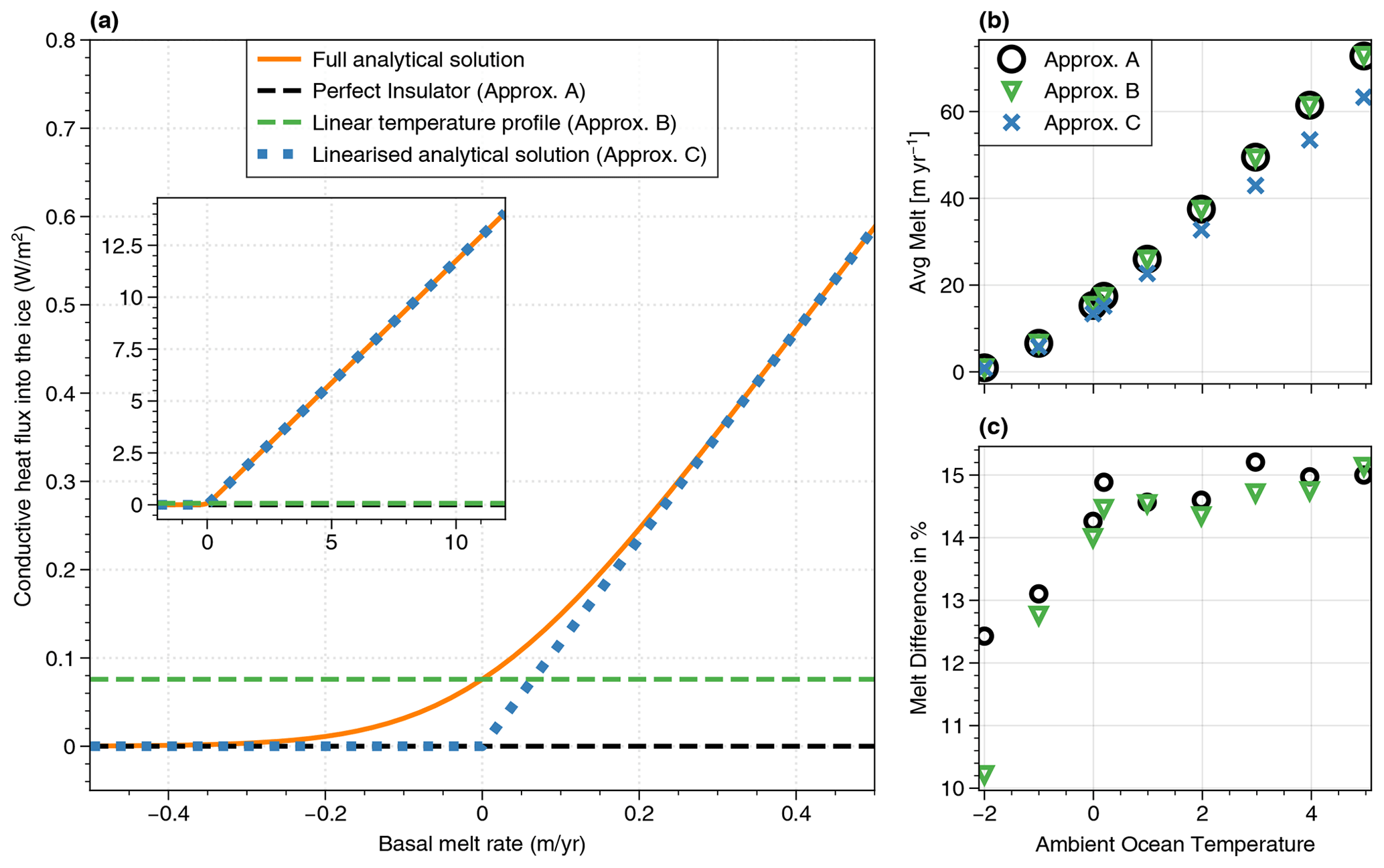
Figure 2 (a) Conductive heat flux at the ice shelf base as a function of the basal melt rate expressed in metres of ice per year. The inset shows the same lines but with a broader range of melt rates. The orange line is the full analytical solution provided by Holland and Jenkins (1999), the dotted blue line is the linear simplification that they suggest (approximation (C) in Eq. 2), and the green line is derived from the assumption of a linear temperature profile across the ice shelf thickness (approximation (B) in Eq. 2). (b) Simulated average melt rate from identical MITgcm ocean simulations of an idealized, 2D Greenland fjord-like domain (Wiskandt et al., 2023) using the three different approximations of Eq. (2) as a function of bottom-layer ocean temperature. (c) Melt rate difference with respect to approximation (C).

If we assume positive melt rates and use Eq. (1), we can estimate the relative difference between approximation (A) and approximation (C):

$$\begin{array}{}\text{(3)}& {\displaystyle }{\displaystyle \frac{\mathrm{\Delta }m}{m}}={\displaystyle \frac{c_{\mathrm{i}}\left(T_{\mathrm{s}}-T_{z_{\mathrm{d}}}\right)}{L}}.\end{array}$$

Considering the parameter values used in Holland and Jenkins (1999), melt rates calculated without considering heat conduction in the ice are overestimated by 11 % for a surface temperature of −20 °C and a freezing point temperature of −2 °C at the ice base. The overestimation is often similar when using the linear temperature profile rather than nothing, except in the absence of basal melting.

Applying Eq. (3) to the observed melt rates in Antarctica gives an idea of where differences in the heat flux estimation have the largest effect on melt (Fig. 3). We use the 40-year (1980–2019) average snow surface temperatures as T_s and calculate the pressure-dependent freezing point temperature $T_{z_{\mathrm{d}}}$ using a typical salinity of 34.6 g kg⁻¹ everywhere. Ice shelves in the Amundsen embayment and the large ice shelves show a difference of around 12 %, with even higher values seen at the Amery Ice Shelf (AmIS) and the eastern RIS (both above 27 %). Under most of RIS this leads to only small differences in absolute numbers (below 0.1 m yr⁻¹, Fig. 3b), since melt rates there are very low (Rignot et al., 2013). In crucial areas, such as close to the grounding lines of the Filchner–Ronne Ice Shelf (FRIS), most of AmIS, and the smaller ice shelves draining towards the Amundsen Sea, the difference is several metres per year, surpassing even 10 m yr⁻¹ at Pine Island Glacier and AmIS. At the calving fronts of FRIS and RIS, melt rate differences are around 1 m yr⁻¹.

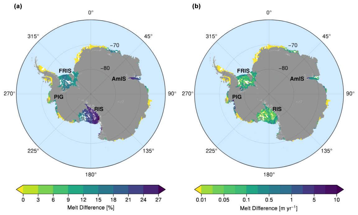
Figure 3 Map of Antarctica showing relative melt rate differences (Eq. 3) between approximations (A) and (C) and respective absolute values when applied to melt rate data for floating ice shelves (b). White areas indicate regions of refreezing.

3 Application to ocean simulations of a small cavity

For a practical implementation of approximation (C) in an ocean model, the criterion on m to bound the heat conduction to zero is not very convenient, as this would require some iterations of the three-equation system because m is a solution that is not known a priori. A more practical solution is to check the sign of the thermal forcing ($T_{\mathrm{w}}-T_{z_{\mathrm{d}}}$ in Eq. 1) to decide whether or not heat conduction is set to zero. This is common procedure for implementing the three equations in ocean modelling. We test this implementation in the MITgcm ocean model (Adcroft et al., 2004) and evaluate whether the relative importance of heat conduction, as derived from theory, is still valid in the presence of a realistic ocean circulation and possible ice–ocean feedbacks.

To show the differences between the three approaches in the melt parameterization in a regional circulation model, we set up a suite of idealized, 2D, and non-rotational simulations (Wiskandt et al., 2023) in the MITgcm with varying ocean temperatures comparing the three different approaches introduced in Eq. (2). The geometry is representative of a long and narrow fjord typically found around Greenland. The domain is 30 km long and 1 km deep with an ice shelf covering the first 20 km of the domain, a grounding line depth of 950 m, and a 50 m deep vertical front. Note that none of the present simulations exhibits refreezing. For all details of the simulation, please refer to Wiskandt et al. (2023).

Given the constant small difference between the conductive heat fluxes from approximations (A) and (B) (Fig. 2a), the simulated melt rates are very similar in these two approximations (Fig. 2b and c). The differences in absolute melt rate are barely discernible to the eye, and the relative differences are <1 % for the simulated temperature range, except for the coldest experiment (Fig. 2c). The difference between approximation (C) and either (A) or (B) is between 10 % and 15 % in most of the experiments. For example, those with temperatures ≥0 °C show a difference of 14 %–15 %.

4 Conclusions

Previous ocean circulation studies at both Greenlandic and Antarctic marine-terminating glaciers implemented approximation (A) (e.g. Gwyther et al., 2020; Comeau et al., 2022) or approximation (B) (e.g. De Rydt and Naughten, 2024; Wiskandt et al., 2023; Holland et al., 2008; Losch, 2008) in Eq. (2) for heat conduction into ice. Combining for the first time a suite of ice temperature profiles representing a variety of melting conditions, we have shown that only approximation (C) estimates the temperature gradient in the ice accurately across the full range of possible melting and refreezing scenarios. We provide a novel map of the local impact of heat conduction parameterization on melt rates in Antarctica and find that approximation (A) overestimates melt rates by up to 25 % (12 % average) compared to approximation (C). Based on Fig. 3a, we can expect a similar overestimation of melt from approximation (B).

We have shown that an inaccurate representation of heat conduction into ice induces biases in melt rates with a high spatial variability. This cannot be corrected by tuning a constant drag or heat transfer coefficient as often done in ocean models. Accurate local melt rates are also crucial for estimating the stability of the ice shelf, e.g. close to the grounding line, where changes in the ice shelf geometry can trigger rapid ice loss (De Rydt and Naughten, 2024). In ocean circulation models, a melt-dependent local temperature gradient is relatively straightforward to implement and, in fact, is available in the MITgcm in the SHELFICE package (Losch, 2008). The Finite-volumE Sea ice–Ocean Model (FESOM2) (Danilov et al., 2017) also uses an approach similar to approximation (C).

We argue here that the parameterization using a linear dependency of the heat flux on the melt rate is the most accurate one. It is nonetheless based on several approximations (Holland and Jenkins, 1999). To accurately model the ice–ocean interactions, a coupled ice sheet–ocean model should be used, with a representation of both vertical and lateral heat conduction and heat advection in the ice (Sergienko et al., 2013). A large number of the current ice sheet models do not however explicitly simulate the ice sheet temperatures and sometimes use approximations of the Stokes equation that prevent a good representation of vertical heat advection in ice. Hence, we suggest that coupled models currently under development should consider calculating the ice sheet temperature gradients or heat fluxes and transfer them to the ocean model to accurately calculate the melt rate using the three-equation system. For non-coupled models, the authors strongly suggest implementing approach (C) of Eq. (2) when parameterizing marine basal melt, as it more accurately represents the heat conduction into the ice and comes at very little additional computational cost.