Insights into supraglacial lake drainage dynamics: triangular fracture formation, reactivation and long-lasting englacial features

Supraglacial lake drainage through fractures delivers vast amounts of water to the ice sheet base, which occurs on timescales of hours. This study is concerned with the mechanisms of supraglacial lake drainage and how a particular area of Nioghalvfjerdsbræ (79° N Glacier), with a lake of a volume of up to 1.23×10⁸ m³, evolved over the last decades. We found extensive fracture fields being formed and vertical displacement across the fracture faces in some instances. The fractures form triangular-shaped moulins, with apertures that are tens of metres wide, into which water flows even after the main lake drainage period. The water level in these moulins may reach the surface and occasionally overflow. These triangular moulin fractures are sometimes reactivated in subsequent years, and their size at the surface remains unchanged for some years, which agrees with viscoelastic modelling. Using ice-penetrating radar, we find englacial three-dimensional features originating from the drainage, changing over years but remaining detectable even years after their formation. The drained water forms a blister underneath the lake, which is released over several weeks. In this area, no lakes existed before an increase in atmospheric temperatures in the mid-1990s, as we demonstrate using reanalysis data. The area is transformed from lake-free to frequent abrupt drainage, delivering massive amounts of lubricant and freshwater at the seaward margin.

1 Introduction

Since the mid-1990s, the Greenland Ice Sheet (GrIS) has been losing mass, with an acceleration of its contribution to sea level rise since the early 2000s (Shepherd et al., 2020). While the mass loss was most prominent in the southern and northwestern parts in the first decade, it has now reached the northeast of Greenland, where the floating tongue of Zachariæ Isstrøm (ZI) disintegrated in 2013 (Khan et al., 2014; Mouginot et al., 2015). Since then, only three floating tongues remain: Petermann Glacier, Ryder Glacier and Nioghalvfjerdsbræ (79° N Glacier, 79NG), with the latter showing the first signs of destabilisation (Humbert et al., 2023b). For floating tongue glaciers, oceanic heat is supposed to be a main driver for thinning and stability (Straneo and Heimbach, 2013; Schaffer et al., 2020), but subglacial freshwater discharge plays a role in this system (Reinert et al., 2023; Zeising et al., 2024). The mass loss of GrIS is attributed to two contributions: (i) glacier acceleration and (ii) changes in surface mass balance, which primarily means an increase in surface melting (van den Broeke et al., 2016; Mouginot et al., 2019). Changes in surface mass balance are a consequence of changes in air temperatures. In the mid-1990s, the weather station Danmarkshavn (76.8° N, 18.7° W) recorded an increase in 2 m temperature of more than 1 °C (Zhang et al., 2022). In this study, we will show that the genesis of a massive meltwater lake coincides with changes in surface temperatures.

The motion of ice sheets and outlet glaciers can be described as gravity-driven lubricated flow. The lubrication can be altered by meltwater that is locally formed in crevassed areas of the ablation zone and is transported through cracks to the glacier base. This can lead to a seasonal acceleration in ice flow via basal lubrication (e.g. Rosenau et al., 2015; Vijay et al., 2019; Neckel et al., 2020). However, the seasonality of glacier speed is not just straight acceleration but exhibits distinct patterns, which depend on the form of the subglacial environment (e.g. Moon et al., 2014). Farther upstream and at higher-elevation locations, the surface meltwater percolates either into the firn matrix or, when the melt onset is too rapid to accommodate complete percolation, into surface runoff. The runoff becomes an organised system of streams and rivers that lead water to topographic depressions where supraglacial lakes may form. These depressions usually correspond to basal topographic lows, and the lakes may range in size from a few square metres to tens of square kilometres. In this study, we focus on a single lake with a size of about 21 km², which we use as a case study.

Supraglacial lakes may drain by either overflowing into pre-existing conduits or through fractures, sometimes denoted as bottom drainage (e.g. Tedesco et al., 2013). This study focuses on drainage through fractures, similar to the studies of Das et al. (2008), Stevens et al. (2015) and Chudley et al. (2019). We use moulin fractures as a term for conduits that are formed by cracking and that are features of a horizontal extent of some tens of metres. In some locations, the ice surface is already highly crevassed when moving into a depression (Neckel et al., 2020). In this case, hydrofracturing (in the sense that a pre-existing crack is water-filled and the crossing of a critical stress threshold triggers the drainage) is the likely drainage mechanism. In other cases, only very shallow pre-existing cracks are present, and fractures are formed during the drainage event. Detailed geophysical studies have revealed that fracture-driven drainage events are rapid and that fractures open to form a water passage and close after the main drainage takes place (Das et al., 2008; Doyle et al., 2013; Stevens et al., 2015; Chudley et al., 2019). It has also been observed that an englacial conduit can remain open over a longer period of time and potentially influence basal melting (Catania and Neumann, 2010). Most in situ observations of englacial systems were conducted outside the large ice sheets (e.g. Fountain and Walder, 1998; Fountain et al., 2005; Gulley et al., 2009). These studies revealed that the englacial systems are often formed by fractures that are initiated in different stress fields.

As fractures are suggested as the origin of englacial pathways, it is important to consider the material behaviour of ice. While ice in glaciers was mainly treated as a viscous fluid obeying non-Newtonian rheology, in recent decades, the solid nature of ice, hence the elastic contribution to deformation, has been explored in more detail (Reeh et al., 2000; Gudmundsson, 2011; Humbert et al., 2015; Christmann et al., 2019, 2021; Rosier and Gudmundsson, 2020). The characteristic of a Maxwell material is that it responds elastically over short timescales, while viscous creep dominates over long timescales. This was found in the 1950s in laboratory studies (Jellinek and Brill, 1956). The solid nature of ice is also the origin of crack formation, which is key for supraglacial lake drainage and englacial channel formation. On the other hand, the fluid nature of ice supports the closure of englacial channels over time.

In this study, we aim to investigate how the drainage of a massive supraglacial lake at 79NG (see Fig. 1) is facilitated, what role fractures play in the drainage and if former drainage systems become reactivated. To this end, we use satellite remote sensing data and data from airborne surveys to investigate lake filling, drainage and englacial pathways of water. We incorporate viscoelastic modelling as a case study to understand if and how drainage pathways close over time. We aim to simulate how a drainage channel at the surface of the glacier would change in size over time. To this end, we employ COMice-ve (https://gitlab.awi.de/jchristm/viscoelastic-79ng-greenland, last access: 5 August 2025), previously used for simulating deformation (Christmann et al., 2021). The lake we focus on is exceptional in size, but more importantly, we built an extensive database from longer-term observations (1985 to 2023).

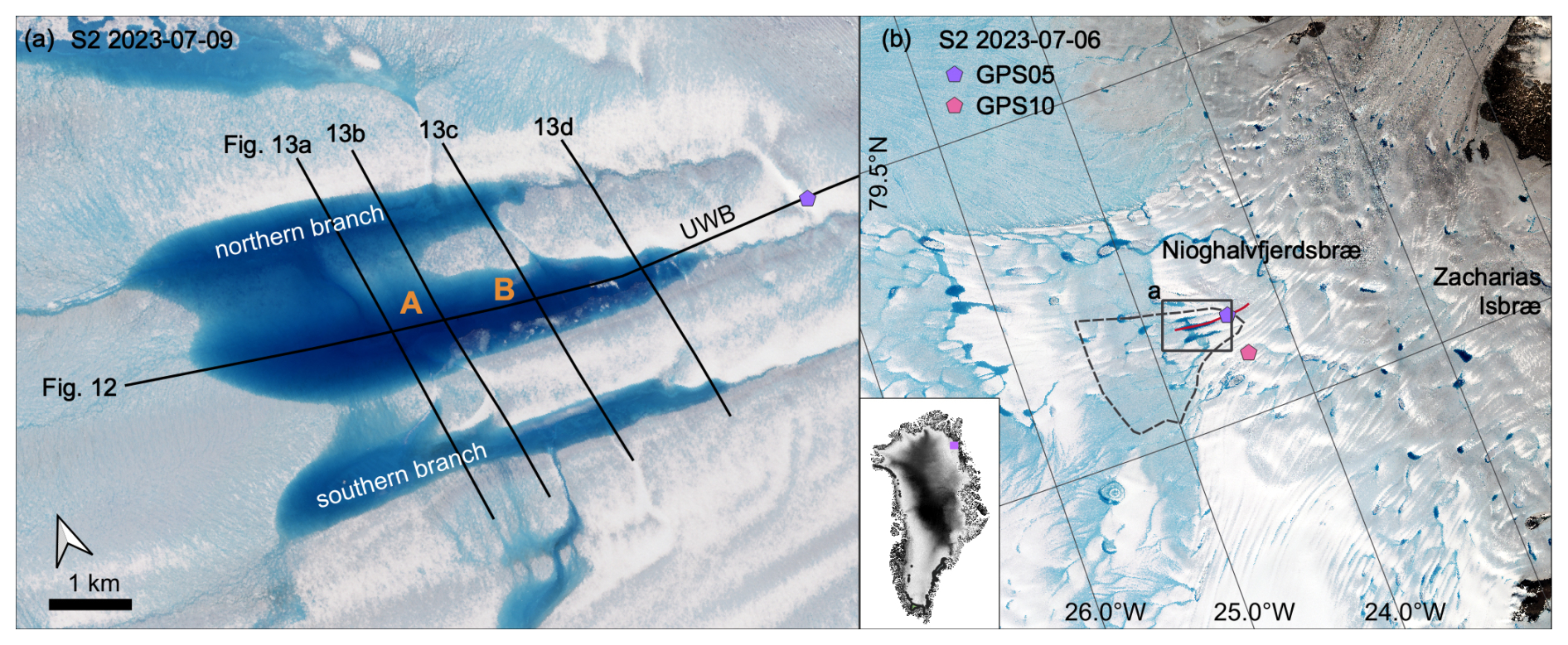
Figure 1 Overview figure. Panel (a) shows the lake on which this study focuses, as seen by S2 on 9 July 2023, with positions of airborne survey crossings as black lines (radar profiles shown in Figs. 13 and 14). Panel (b) gives a wider overview of the region. Superimposed onto the S2 scene from 6 September 2023 is the area for the CARRA (Schyberg et al., 2020) subset, shown in Fig. 16 as a dashed line and the GNSS positions presented in Fig. A1 as pink and purple symbols. The inset shows the location of panel (b) in Greenland.

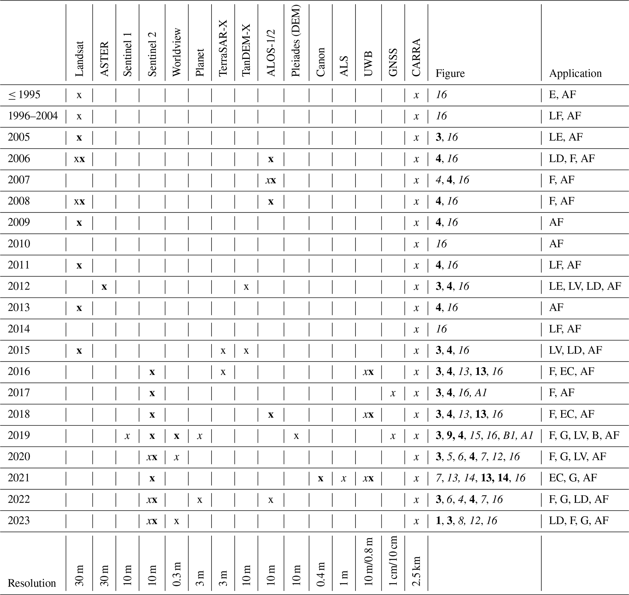
The article is structured as follows: we first present the methods and give an overview of the extensive database and the model. Subsequently, we present the results from observations, followed by the simulations. A discussion and a synthesis of data and modelling continue this. As we use data from various sources for several purposes, we provide a comprehensive overview in Table 1.

Table 1 Overview of the data used in this study in respective years. The bold font refers to the appearance within the article. x denotes that the data are shown in a figure; x indicates that we used this data to extract a feature (e.g. a line, a moulin fracture position), which is shown in a figure; and x shows that the data are used to draw information or a conclusion that is discussed in the text only. B = blister, E = existence, EC = englacial channel, F = fracture, G = triangular moulin fracture, LD = lake drainage, LE = lake extent, LF = lake filling, LV = lake volume, AF = atmospheric forcing. The last line presents the resolution. If two numbers are given, the first is the horizontal resolution and the second is the vertical resolution.

2 Data and methods

2.1 Satellite data and method

2.1.1 Optical satellite data

We use optical satellite imagery from different missions: (1) in medium-resolution (10 m) S2 (S2) imagery for time series and (2) in high-resolution WorldView2 imagery (1.2 m multi-chromatic, 0.3 m panchromatic) for snapshots in time to measure the geometry of the drainage pathways and to detect the crack locations. (3) We use Landsat and ASTER data to extend the time series. All data available in the Landsat, ASTER and Sentinel archives were manually quality-assessed, and only acceptable quality and cloud cover images were used in this study. Sentinel-2 (S2) MSIL1C products have been processed using the European Space Agency's (ESA's) SNAP toolbox. We use bands 2, 3 and 4 to obtain RGB images. The original data were projected onto the resolution of band 2. Most of the imagery we use here is cloud-free, but in some circumstances we need to use imagery that contains some cloud cover. We use WorldView imagery from 23 August 2019, 19 August 2020 and 1 August 2023 in the panchromatic mode. The data have not been further processed and are used in the original resolution.

2.1.2 Radar satellite data

We used ALOS-1 and ALOS-2 data to identify fractures and moulins. In 2006, we used one ALOS-1 single-polarisation data acquisition to detect fractures formed during lake drainage since no dual- or quad-pol data were available. ALOS-1 quad-pol data have been used in this study to detect the locations of fractures and drainage features for 2007 and 2008. We applied a Pauli decomposition using the Gamma software package (released 1 December 2023). The processing includes radiometric correction, multi-looking and georeferencing the Arctic digital elevation model (DEM) before the Pauli decomposition. The resulting product has a 20 m pixel resolution and contains single scattering, double scattering and volume scattering as three bands. The ALOS-2 data used in this study are only dual-pol data; thus, no full Pauli decomposition could be applied. Here, we use the different polarisations HH, HV and HH-HV as three bands to identify fractures and drainage features. We used the TerraSAR-X product, acquired in stripmap mode and enhanced ellipsoid corrected (EEC). We conducted a bi-cubic interpolation for speckle reduction to a 12.5 m resolution.

2.1.3 Maximum lake area

We digitised the lake outlines before the drainage event (shown in Fig. 3a), based on the last available imagery before major drainage: 20 July 2005 (Landsat), 25 July 2012 (ASTER), 24 July 2015 (TSX), 26 July 2019 (S2), 13 August 2021 (S2), 13 August 2022 (S2) and 9 July 2023 (S2).

2.1.4 Lake volume estimate

To estimate the water volume of the supraglacial lake, we generated three digital elevation models (DEMs) for the empty lake basin. While two DEMs originate from TanDEM-X data, acquired on 16 May 2012 and 2 November 2015, the third DEM was generated from Pleiades data, acquired on 11 May 2019. TanDEM-X DEMs were generated using SAR interferometry, as described by Neckel et al. (2013), and the Pleiades DEM was derived by stereo photogrammetry employing NASA's Ames stereo pipeline (Beyer et al., 2018). All DEMs were horizontally and vertically adjusted to the global TanDEM-X DEM (Wessel et al., 2016) near the lake using the pc_align utility provided within the Ames stereo pipeline. From the DEMs, we picked shoreline elevations, employing the closest available optical satellite scenes of the filled lake. For this, we used an ASTER satellite scene acquired on 23 July 2012, a Landsat-8 scene acquired on 24 July 2015, and two S2 scenes acquired on 27 July 2019 and 14 July 2020. After filling the lake basin, we calculated the difference between the picked shoreline elevations and the respective DEM of the empty lake. From the integrated differences, we estimated the total water volume of the lake on the four dates of optical satellite acquisitions.

2.1.5 Surface subsidence maps

To estimate surface subsidence in the vicinity of the lake, we will make use of additional Sentinel-1 SAR acquisitions. We employed Sentinel-1 Interferometric Wide Swath (IW) Single Look Complex (SLC) data acquired in 2017 and 2019. Interferograms were formed by calculating the phase difference between two Sentinel-1 acquisitions of the same satellite orbit separated by 6 d. The topography-induced phase difference was cancelled with the help of the global TanDEM-X DEM (Wessel et al., 2016). The remaining interferometric phase is mainly attributed to vertical and horizontal surface displacement projected into the line of sight (LOS) of the satellite (e.g. Rignot et al., 2011; Friedl et al., 2020; Neckel et al., 2021). To cancel the horizontal ice movement, we employed one master interferogram, including data acquisitions from 2 October 2019 and 8 October 2019. Hence, we attribute the remaining phase difference solely to the vertical surface displacement between the August and September 2019 data acquisitions. Depending on the magnitude of the surface displacement and the coherence of the interferograms, unwrapping can be challenging in some cases, requiring different strategies for absolute estimates of surface displacements. In these cases, we employed speckle-tracking methods on the same data acquisitions as used for interferometry (e.g. Joughin et al., 2016a). Finally, the unwrapped interferometric estimates and the speckle-tracking-derived fields were projected from the LOS direction to the vertical, representing short-term variations in vertical surface displacement (Fig. 15).

2.2 In situ data

2.2.1 Ground-based GNSS

Two dual-frequency Novatel GNSS receivers were deployed in the 2017 field season to measure the horizontal and vertical displacement of the glacier surface over time. The receivers collected data for roughly 2 years, with some data gaps occurring during winter. The flow trajectory was computed using the precise point positioning (PPP) post-processing option, which included precise clocks and ephemerides of the commercial GNSS Waypoint software package (version 8.90). The accuracy of the post-processed trajectory is better than 0.02 m. Based on the trajectories, we could estimate temporal variations in the ice flow velocity and vertical displacements after lake drainage events.

2.3 Airborne methods

The airborne data were acquired in three campaigns. The dates of the survey flights were 27 June 2016, 11 April 2018 and 29 July 2021. The corresponding flight lines can be viewed in the online radar data viewer of the Alfred-Wegener-Institut Helmholtz-Zentrum für Polar- und Meeresforschung (AWI, https://marine-data.de/viewer/d181f76f-fa15-44c9-8452-07540c72e0be, last access: 5 August 2025). The last campaign was dedicated to englacial reflections, and the lake was surveyed in more detail than in the prior campaigns. The transects we used here are only parts of the entire campaigns.

2.3.1 Airborne GNSS

For georeferencing the optical imagery, laser scanner and radar data, the aircraft position was measured using a dual-frequency NovAtel OEMV GNSS receiver with a sampling rate of 20 Hz. The flight trajectory was computed using the PPP post-processing option, which included precise clocks and ephemerides of the commercial GNSS Waypoint software package (version 8.90). The accuracy of the post-processed trajectory varies along the track but is better than 0.1 m.

2.3.2 Airborne optical camera

On board AWI's research aircraft, a Canon EOS-1D Mark III digital single-lens reflex (DSLR) camera, in combination with a Canon 14 mm f/2.8L II USM lens, is routinely employed. Images were acquired in 6 s intervals and stored with a GNSS time tag in RAW data format. All images were corrected for vignetting effects. During the conversion to JPG format, the original resolution was preserved. The images were geocoded using the post-processed GNNS trajectory in combination with the aircraft attitude data.

2.3.3 Airborne laser scanner

During the same flight on 29 July 2021, laser scanner data were acquired using a RIEGL LMS VQ-580 with a scan angle of 60° at about 300 m flight height, which results in a width of the footprint of about 300 m. The mean point-to-point distance is ∼0.5 m. The raw laser data were combined with the post-processed GNSS trajectory and corrected for aircraft altitude and calibration angles using AWI's laser scanner processing software, leading to calibrated georeferenced point cloud (PC) data. We used crossovers to calibrate the system and to derive the elevation accuracy. The georeferenced PC has an accuracy better than 0.1 ± 0.1 m. The bias is <0.1 m and varies along the track. It arises from the vertical accuracy of the post-processed GNSS trajectory. The resulting DEM was derived from the PC using an inverse distance weighting (IDW) algorithm and a 5 m search radius. Its resolution is 1 m in the horizontal direction. The elevation was referenced to the EGM2008 geoid (Pavlis et al., 2012).

2.3.4 Airborne ice-penetrating radar

This study used an ice-penetrating radar to determine the glacier's internal structure. The data were acquired using AWI's ultrawideband (UWB) Multichannel Coherent Radar Depth Sounder (MCoRDS, version 5), with an array of eight antennas (Hale et al., 2016). The total transmit power is 6 kW. In our survey, we used a bandwidth of 370 MHz within the frequency band of 150–520 MHz. The radar was operated with a pulse repetition frequency of 10 kHz and a sampling frequency of 1.6 GHz. The dynamic range was increased using alternating sequences of different transmission (recording) settings (waveforms). Short pulses (1 µs) and low receiver gain (11–13 dB) are used to image the glacier surface. Longer pulses (3 and 10 µs) with higher receiver gain (48 dB) are used to image the internal features and the ice base. The waveforms are defined, considering the glacier's ice thickness. Data processing was performed using the CReSIS toolbox. It included a pulse compression in range direction and synthetic aperture radar focusing on the along-track direction, which leads to an along-track resolution of 10 m. A relative permittivity of ε_r=3.15 in ice was used for the time-to-depth conversion. The survey area is in the ablation zone. Thus, we assume no extensive firn layer to be present. Therefore, we did not apply any firn correction. After pulse compression, the theoretical range resolution is about 0.23 m. In the last processing stage, the echograms of the two waveforms were concatenated into one radargram, covering the ice from the surface to the base with a high dynamic range. This has been done for all flight segments on 29 July 2021 in along-flow and across-flow directions.

2.4 Reanalysis data

2.4.1 Copernicus Arctic Regional Reanalysis (CARRA)

To investigate the impact of the atmospheric forcing on the lake formation, we analysed the summer skin temperatures for June, July and August between 1991 and 2022 using the CARRA system (Schyberg et al., 2020). The skin temperature represents the temperature of the uppermost surface layer that responds instantaneously to changes in surface fluxes. The product of this analysis consists of daily skin temperatures at 15:00 UTC with a horizontal resolution of 2.5 km. We averaged the daily skin temperature in the lake's drainage basin and calculated the daily 5-year median temperature, with shorter intervals for the first (1991–1994) and last periods (2020–2022).

2.5 Modelling methods

2.5.1 Viscoelastic modelling

To simulate the radial horizontal displacement of the englacial channel at the top surface of the glacier, we chose a two-dimensional top view and modelled the system as a rectangular disc with a circular hole. From this point of view, gravity is not taken into account. Thus, the statement of the local equilibrium reads

$$\begin{array}{}\text{(1)}& \text{div}\mathit{\sigma }=\mathrm{0},\end{array}$$

with the Cauchy stress tensor σ. We confine our calculations to small deformations. From the two-dimensional displacement vector $\mathit{u}=(u,v{)}^T$, the linearised strain tensor ε is derived as

$$\begin{array}{}\text{(2)}& \mathit{\epsilon }={\displaystyle \frac{\mathrm{1}}{\mathrm{2}}}(\mathrm{\nabla }\mathit{u}+(\mathrm{\nabla }\mathit{u}{)}^T).\end{array}$$

For polycrystalline ice, the established rheological model is the Maxwell material, as introduced by Christmann et al. (2021). This material shows instantaneous elastic deformation as well as time-dependent viscous creep. A series of springs and dampers is the one-dimensional mechanical equivalent to the Maxwell material. In the multi-dimensional case, the volumetric stress is related to reversible elastic volume changes and is, therefore, not time-dependent. We decompose the stress and strain tensors into a volumetric and deviatoric part by performing $(\cdot {)}^D=(\cdot )-\mathrm{1}/\mathrm{3}\text{tr}(\cdot )\mathbf{I}$, with the trace operator tr(⋅) and the second-order identity tensor I. The material behaviour can be described by using only the time-dependent deviatoric parts. For the Maxwell material, the total deviatoric strain comprises an elastic (⋅)_e and a viscous (⋅)_v part as

$$\begin{array}{}\text{(3)}& {\mathit{\epsilon }}^D={\mathit{\epsilon }}_{\mathrm{v}}^D+{\mathit{\epsilon }}_{\mathrm{e}}^D.\end{array}$$

The deviatoric stress in the viscous element with viscosity η equals the deviatoric stress in the elastic element with shear modulus μ and reads

$$\begin{array}{}\text{(4)}& {\mathit{\sigma }}^D=\mathrm{2}\mathit{\eta }{\dot{\mathit{\epsilon }}}_{\mathrm{v}}^D=\mathrm{2}\mathit{\mu }{\mathit{\epsilon }}_{\mathrm{e}}^D,\end{array}$$

with the time derivative $\dot{(\cdot )}=\mathrm{d}(\cdot )/\mathrm{d}t$. Inserting Eq. (3) into Eq. (4), we obtain the evolution law for the deviatoric strain:

$$\begin{array}{}\text{(5)}& \mathit{\mu }({\mathit{\epsilon }}^D-{\mathit{\epsilon }}_{\mathrm{v}}^D)=\mathit{\eta }{\dot{\mathit{\epsilon }}}_{\mathrm{v}}^D.\end{array}$$

The resulting stress to fulfil the equilibrium statement Eq. (1) follows from the material law of the elastic element as

$$\begin{array}{}\text{(6)}& \mathit{\sigma }=K\text{tr}\left(\mathit{\epsilon }\right)\mathbf{I}+\mathrm{2}\mathit{\mu }{\mathit{\epsilon }}_{\mathrm{e}}^D,\end{array}$$

with the bulk modulus $K=E\mathit{\mu }/\left(\mathrm{3}\right(\mathrm{3}\mathit{\mu }-E\left)\right)$, where E is the elastic Young's modulus.

The system of equations is solved with the finite-element software COMSOL Multiphysics (version 5.4). For the simulation, we chose typical values for polycrystalline ice, such as

$$\begin{array}{c}{\displaystyle }E=\mathrm{9}\mathrm{GPa}\\ {\displaystyle }\mathit{\mu }=\mathrm{3.396}\mathrm{GPa}\\ {\displaystyle }\mathit{\eta }=\mathrm{3}\times {\mathrm{10}}^{\mathrm{14}}\mathrm{Pa}\mathrm{s}\\ {\displaystyle }{p}_{\mathrm{0}}=\mathrm{1}\times {\mathrm{10}}^{\mathrm{5}}\mathrm{Pa}\text{ for }\mathrm{0}<t<\mathrm{10}\mathrm{d}.\end{array}$$

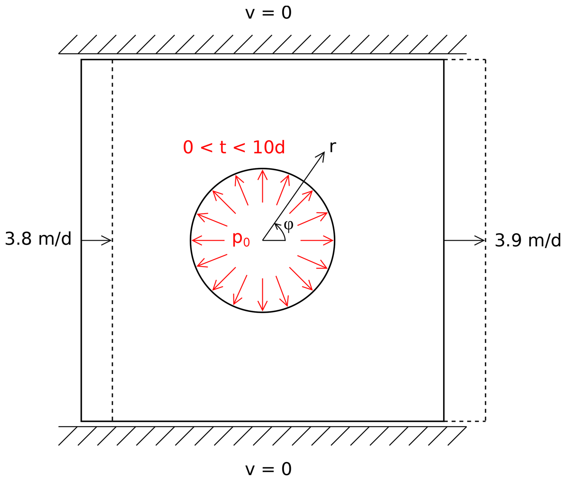
The edge length of the rectangular disc is 20 km, and the radius of the hole is chosen to be 20 m (Fig. 2). A horizontal displacement is applied for every time step t on the boundaries to model the accelerated ice flow. As the left boundary condition, we chose $\mathrm{3.8}\mathrm{m}{\mathrm{d}}^{-\mathrm{1}}\cdot t$, in accordance with remote-sensing-based velocities, and on the right boundary $\mathrm{3.9}\mathrm{m}{\mathrm{d}}^{-\mathrm{1}}\cdot t$. The upper and lower boundaries are fixed in the vertical direction but can move freely in the horizontal direction. The water pressure inside the channel before and after drainage is modelled by applying traction in the radial direction. The traction is applied for 10 d and then set to zero for another 10 d to simulate the small deformations during the immediate drainage event.

Figure 2 Coordinate system and boundary conditions for disc and hole.

2.5.2 Inversion modelling

We employ an inverse model similar to the one in Humbert et al. (2023a) in order to obtain principal angles. We leverage the Ice sheet and Sea-level System Model (ISSM; Larour et al., 2012) to simulate the ice dynamics around the supraglacial lake in 3-D using higher-order approximation (Blatter, 1995; Pattyn, 2003). The bed and surface topography is from BedMachine Greenland (version 4) (Morlighem et al., 2017; Morlighem et al., 2021). The mesh resolution beneath the subglacial lakes is around 500 m. The mesh is vertically extruded into 15 layers that are refined near the base. We infer the basal friction coefficients under the grounded ice through inversions following Morlighem et al. (2013), utilising surface velocities of the MEaSUREs dataset (Joughin et al., 2010, 2016b). A cost function is minimised to match the target velocity during the inversion process. An L-curve analysis was performed to select the optimal parameters for the inversion to avoid overfitting or overregularisation. The thermal regime is assumed to be in a steady state. We ensure that velocities and temperatures are consistent by running a thermomechanical steady state until both fields converge. At each inversion iteration, we compute the ice temperature and update the ice hardness accordingly to ensure consistent ice flow and thermal regimes. Therefore, the initial temperature computed is based only on present-day conditions and does not include past climate history. This approach is similar to that used by Seroussi et al. (2013) but with an improved description of the enthalpy scheme (Rückamp et al., 2020; Kleiner et al., 2015; Aschwanden et al., 2012). Stresses in a Cartesian coordinate frame are computed from velocity gradients and ice viscosity at the surface following Eq. (4). These stresses are then rotated to match the principal direction.

3 Results

3.1 Supraglacial lake genesis and drainage characteristics

In the following, we present the results from the satellite imagery, which is the most extensive part of this section. Subsequently, we will show observations from the airborne survey. Lastly, we will provide data on atmospheric forcing. The intention is to present the evolution of this lake from the beginning to its current state.

Although the data coverage in the 1980s and 1990s is sparse, no lake was observed having formed in the observational data until 1995. It took about 10 years until the first drainage occurred (see Table 2). Figure 3 presents the lake extent before drainage. The lake area before the first drainage was the largest on record. The timing of the drainage can be constrained to the fall of 2005 and June 2006, as the lake surface in a Landsat image acquired on 3 June 2006 (not shown) was no longer a flat, snow-covered area. In the ALOS-1 L-band imagery from 3 April 2007, almost a year later, we find line-shaped cracks and triangular features (Fig. 4).

Table 2 Timing of start and completion of filling and drainage.

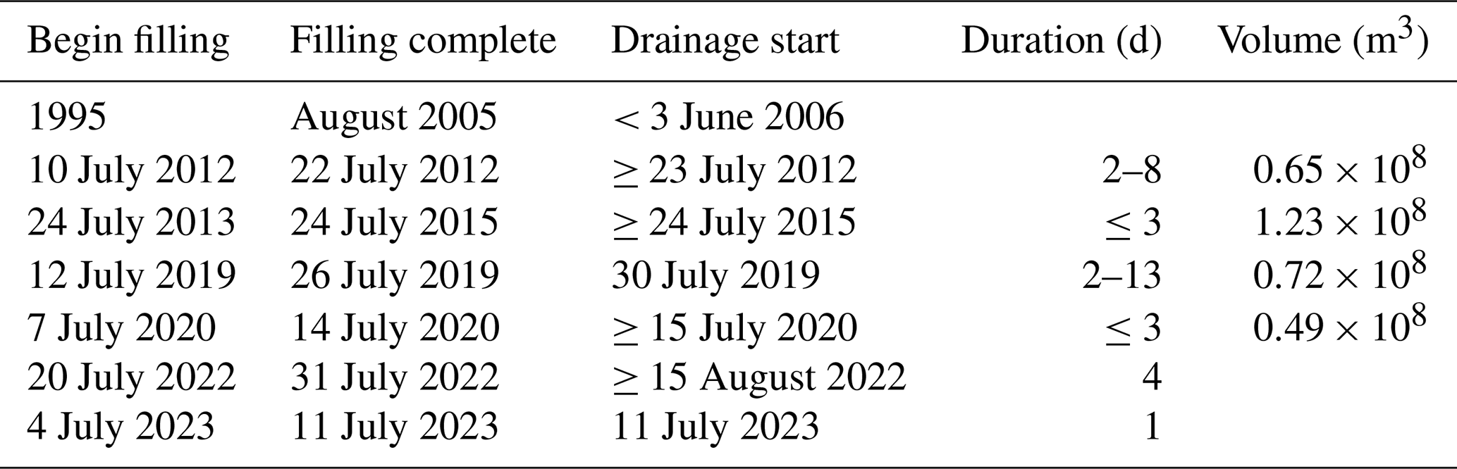
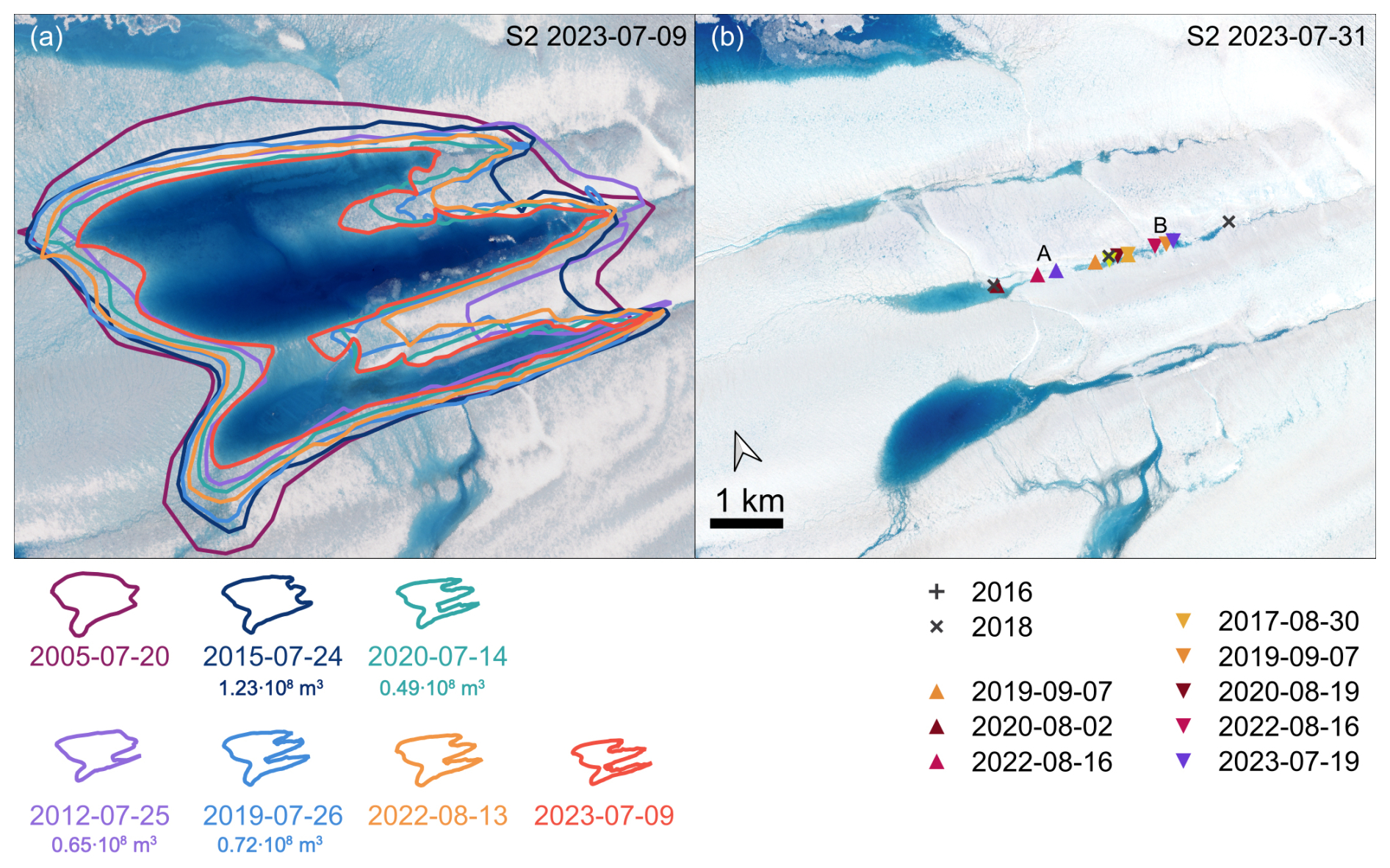
Figure 3 (a) Maximum lake extent before lake drainage for all drainage events (coloured lines) superimposed over S2 imagery from 9 July 2023. (b) S2 imagery from 31 July 2023 after lake drainage. Triangular moulin locations in areas A and B are shown as triangles. The colour corresponds to the year of the moulin's formation. Grey crosses mark locations with englacial reflections in the UWB radargrams (Fig. 13) in 2016 and 2018. The volume of the lake before drainage is given below the dates.

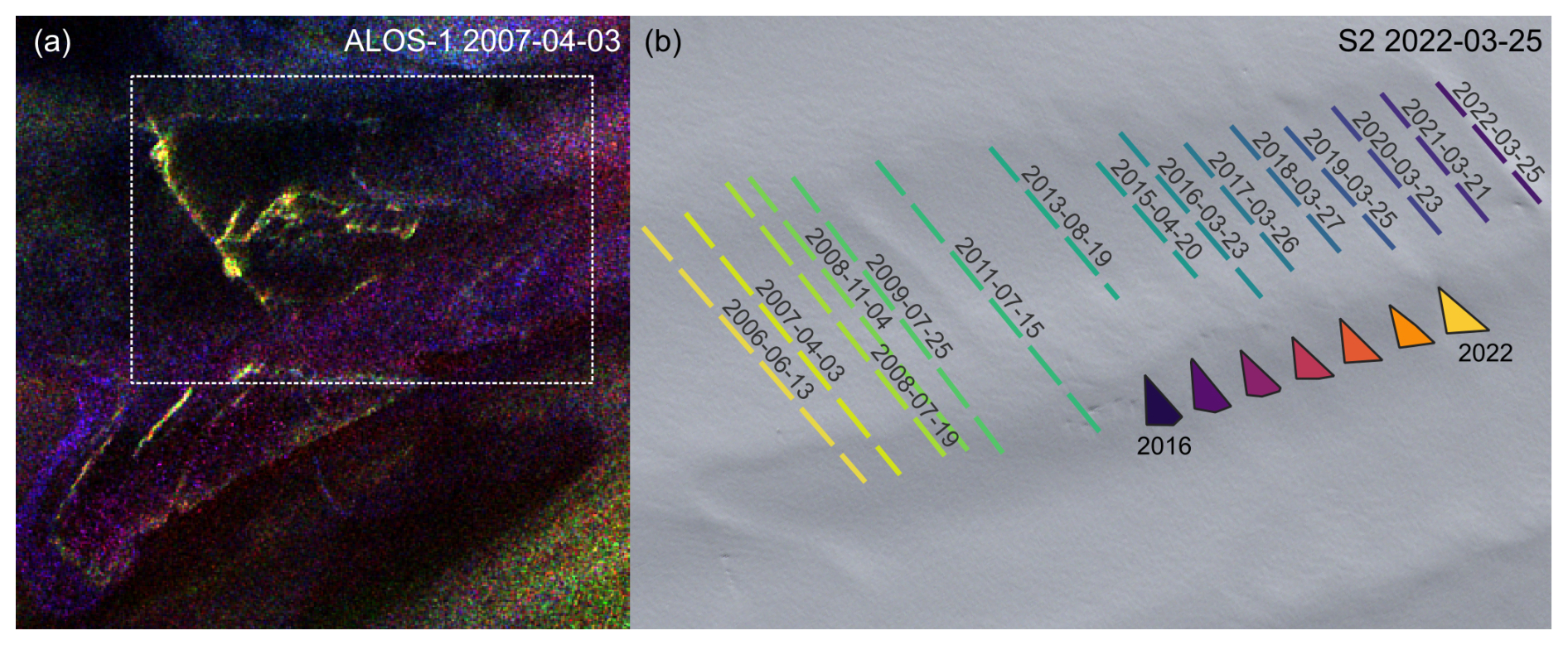
Figure 4 Panel (a) displays a Pauli decomposition from an ALOS-1 quad-pol acquisition (© JAXA (2007)) on 3 April 2007. Panel (b) displays an S2 image on 25 March 2022 in the background. Coloured lines denote the fracture from the 2005/2006 drainage event and its evolution over time. Note the shade of the background image of the last dashed grey line, which indicates a topography step. Coloured triangles mark the triangular-shaped feature from the 2015 drainage event that remains visible in subsequent years in optical imagery, although with a fading appearance.

The second drainage occurred in 2012 between 23 July and 26 July (ASTER). The lake extent before drainage was 32 % smaller than in 2005 (Fig. 3a).

In 2013, the middle branch of the lake filled but no drainage occurred, indicating that the drainage pathways from 2012 were shut. At the end of August, the lake's surface froze over. In the summer of 2014, the lake filled but no drainage occurred. The lake's surface froze over at the end of summer 2013 and 2014. In 2015, the third drainage took place between 24 July 2015 (Fig. 3a) and 27 July 2015 (Landsat, not shown). The drainage occurred while the lake was still covered with ice, preventing drainage fracture analysis. However, together with the drainage, cracks were formed (also clearly visible in a TSX acquisition on 4 August 2015, not shown), which are discussed in the section below. At the end of August (26 August 2015, not shown), an overflow from a northern lake is found in TSX imagery. In 2016, the lake did not fill entirely, although some melting occurred (visible in S2 imagery, which we do not display here). This is consistent with a still open and active drainage system. The TSX imagery of 21 July 2016 (not shown) exhibits open water in the northern, central and southern branches. In the central branch, the shape of the ponding is comparable to other years but has an ending in the form of a 155 m long line. On 9 September 2016, a hole was visible at the southern end of that line. It is the first feature that we identify as a triangular moulin fracture. It is located in area B (see Fig. 1b) and shown in Fig. 3b. In S2 imagery, surface cracks and drainage features are visible, which will be discussed below. In 2017, melting started late and filled the lake from 26 July 2017 with a small amount of water. The peak was reached on 1 August 2017, with a reduction in the northern branch on 2 August 2017 (both not shown here). The GNSS data show a velocity increase between 31 July 2017 and 6 August 2017 of about 10 % (Appendix A). The moulin in area B has moved with the speed of the glacier (yellow mark for 30 August 2017 in Fig. 3b). The year 2018 had a rather cold summer in which no substantial melting occurred at the lake's elevation. A nearby GNSS station was covered with snow the entire summer. The S2 scenes do not show any meltwater, and ALOS-2 data do not exhibit any new signs of fracture. The fourth drainage event happened in 2019: the largest lake extent in 2019 was found on 26 July 2019 (Fig. 3a), again smaller than in 2005, 2012 and 2015. The S2 acquisitions cover the drainage. While the lake was still filled on 30 July 2019 (not shown), the scene from 31 July 2019 (not shown) shows that the lake volume reduced drastically, but deeper areas were still filled. One drainage location can be identified, which we denote as location A (Fig. 3b). This moulin fracture at location A can, however, only be inferred due to the ponding at the end of summer – 22 August 2019 (S2) – which has a form that is consistent with a drainage pathway at this location. Also, in WorldView on 23 August 2019, this location is the end of a water body, as shown in Fig. 10. It looks as if the water has been flowing into a triangular hole with 54, 44 and 67 m edge lengths formed by cracks, and it appears visually deeper than the surroundings. Moreover, an S2 scene from 22 August 2019 shows a concentration of cracks around a spot that we denote as location B (Fig. 3b). This image also reveals a crack 1060 m downstream of the moulin fracture in region A that year, which was not the main drainage location in 2019. Drainage event number five occurred in 2020, the first one just 1 year after a prior drainage event. The lake was filled on 14 July 2020 (Fig. 6a), just 7 d after it started to fill. Only 1 d later, on 15 July 2020, a large amount was drained, but drainage continued until 17 July 2020. It is mainly drained, although the southern branch still contains a significant amount of water. A triangular-shaped moulin in the 10 m resolution S2 imagery is most striking. On 19 August 2020, a high-resolution scene (WV) was acquired, as displayed in Fig. 5. At the location of the moulin fracture, visible a month before in the S2 imagery, a triangular-shaped area is filled with water (230, 213 and 170 m side lengths), and a heap of ice blocks is found (the largest block measures 6 m in width). Outside this moulin, southeast of the heap, larger ice blocks are found (the closest is 318 m away from the moulin). The largest one measures 20 m in width, and the majority are in the order of 10 m in width. At the end of summer, the central branch of the lake is drained entirely, and the southern branch drained between 10 August 2020 and 15 August 2020 (Fig. 6b). Only the northern branch contains some water, which appears to come from an overflow of the neighbouring lake. The meltwater in the summer of 2021 did not lead to a complete refilling, and besides some water ponds in the middle branch, no drainage took place by the end of summer. The 2021 survey (UWB, ALS and Canon camera, 29 July) showed that the moulin had the same horizontal geometry as in 2019 (Fig. 7c and d), although the triangular feature has snow cover. Laser scanner data reveal this corner to be 16 m deeper than the surrounding surface. Note that this is not the actual depth of the englacial channel, as the flight elevation and speed do not allow for a sounding of the depth. Just 1 d later (30 July 2021), S2 imagery shows that the lake ice is entirely melted and the width of the ponding area at area A is 278 m. By 8 August 2021, this width is reduced to 96 m at the same location. The moulin at location A-2020 has moved between 19 August 2020 and 2 September 2021 by 297 m, consistent with a glacier velocity of 290 m a⁻¹. At location B, the drainage channel is still “blocked” with ice fragments and is elevated about 1 m higher than the surrounding lake area, underlining the finding that the ice fragments piled up.

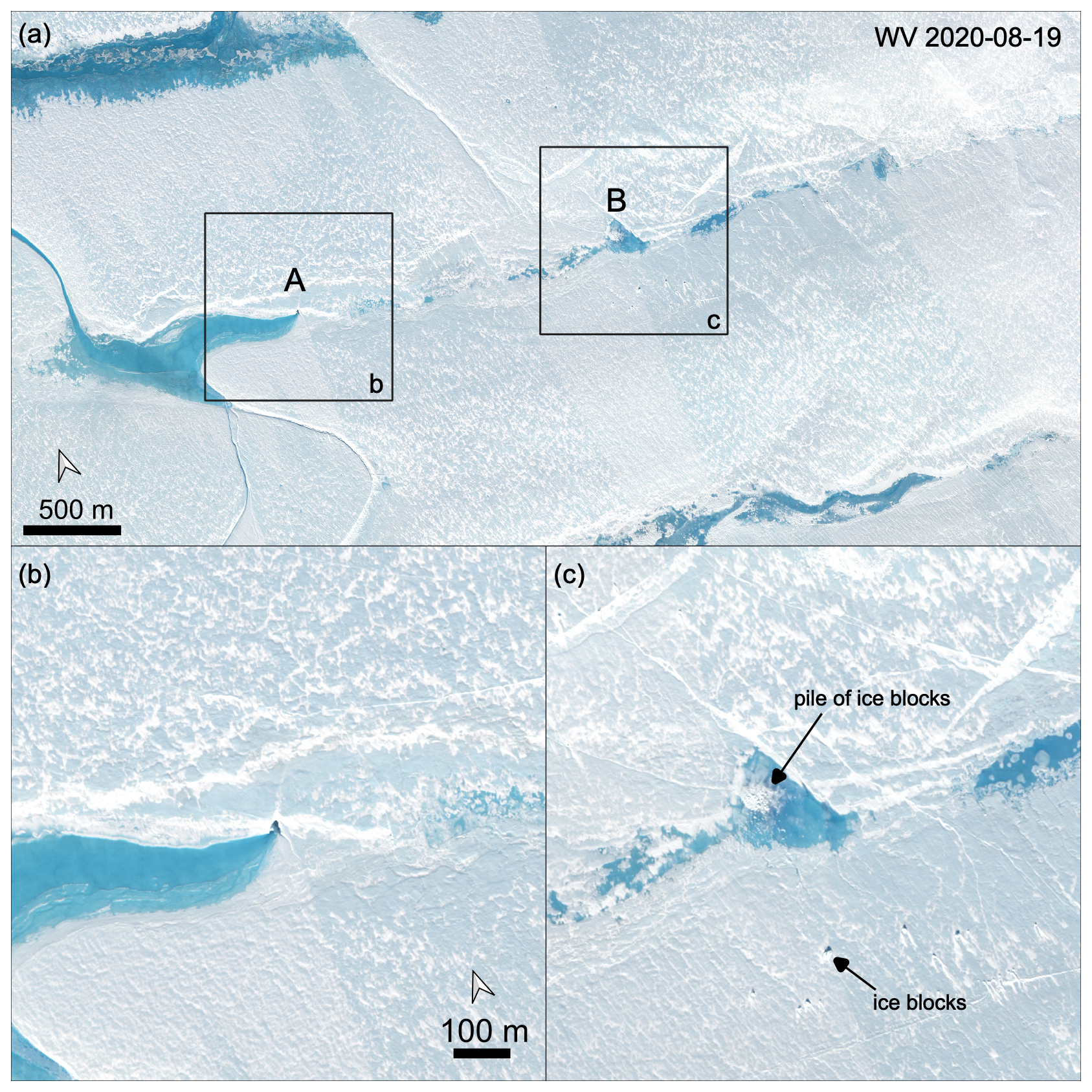
Figure 5 Triangular moulin fracture in the drainage event in 2020. The high-resolution image is a multi-chromatic WorldView image (© DigitalGlobe, Inc. (2020), provided by European Space Imaging) acquired on 19 August 2020. Panel (a) displays the central branch of the lake and indicates the location of the two areas of panels (b) and (c).

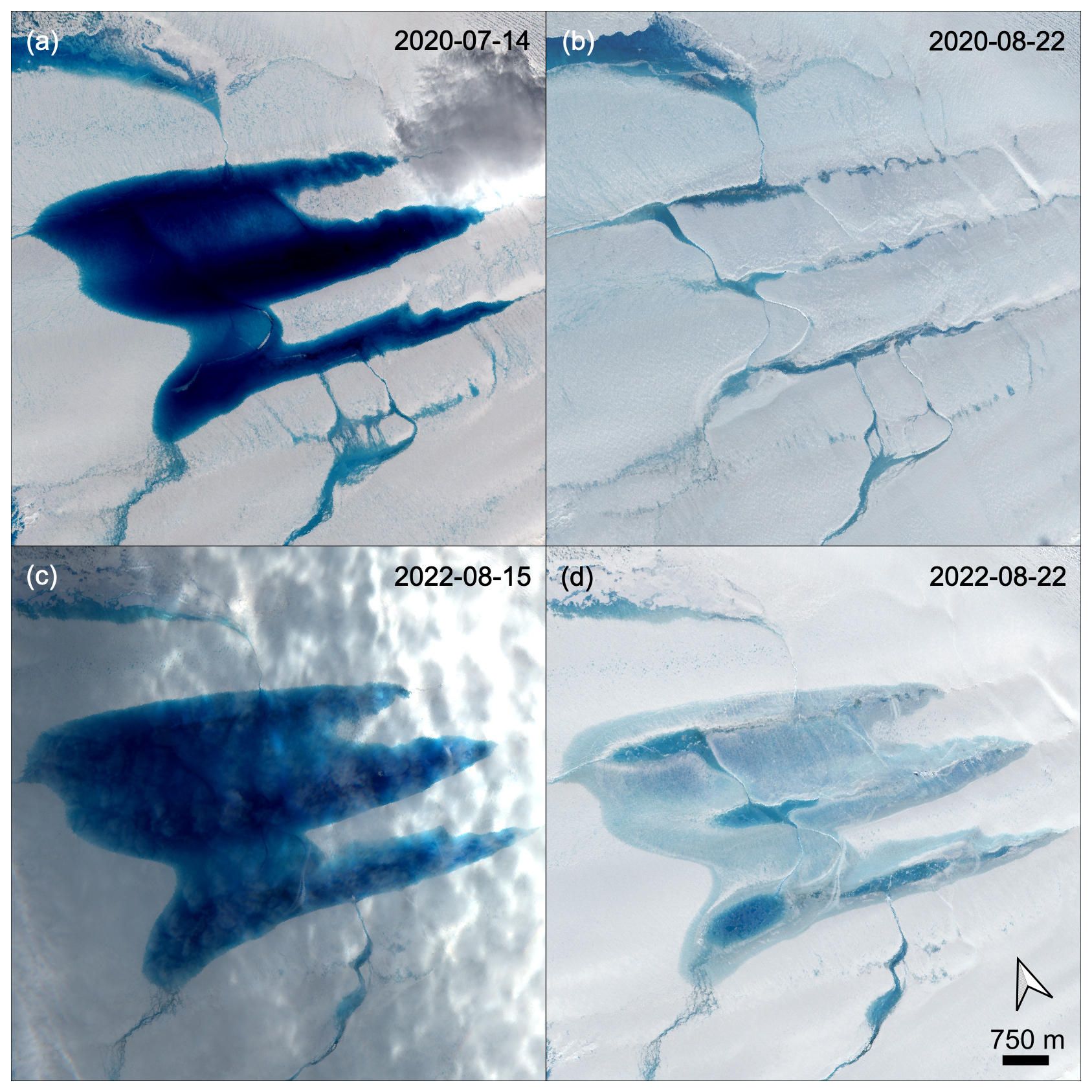
Figure 6 S2 images before and after drainage: (a, c) lake filling on the last day before drainage and (b, d) the last day of the season after drainage.

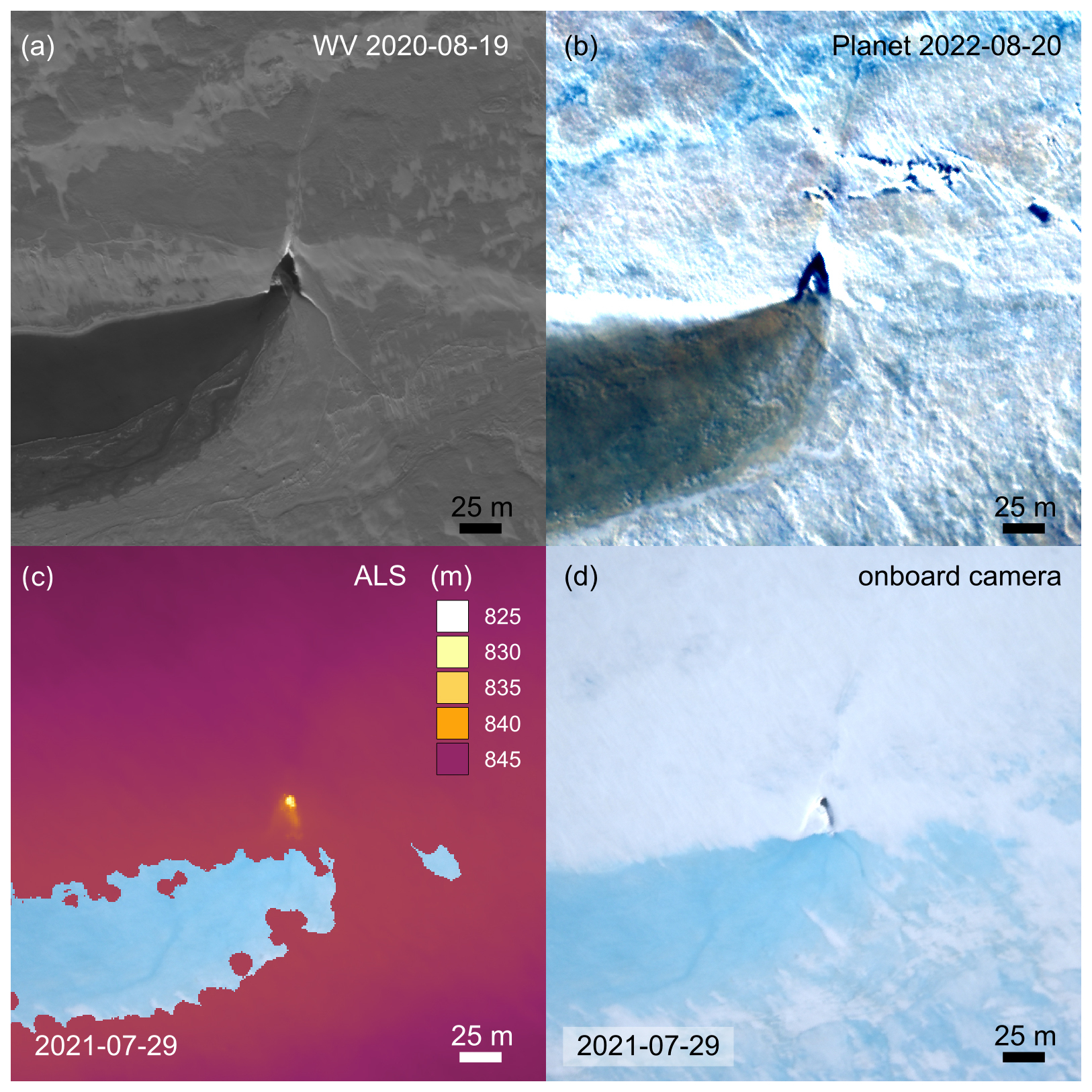
Figure 7 Panels (a) and (b) show the triangular moulin fracture at location A (Fig. 3) in high resolution. Panel (a) is a pan-chromatic WorldView image (© DigitalGlobe, Inc. (2020), provided by European Space Imaging) and panel (b) displays a multi-chromatic Planet image (© Planet (2025)). The time between the two high-resolution images is 2 years, and the geometry of the triangular feature remains the same. In panel (c), the topography of the surface is shown, while panel (d) shows the synchronous optical imagery of the Canon onboard camera.

In 2022, the moulin at location A was visible in the filled lake in the S2 imagery for several days before the lake drainage. At location B, we identified some floating ice blocks near the drainage channel on 15 August 2022 (Fig. 6c; the scene is unfortunately cloudy). A day later, the lake drained substantially. Ice blocks are visible next to the drainage channel at location B. High-resolution imagery from 20 August 2022 (4–5 d after drainage) reveals that the size of the triangular moulin in area A is about the same as in 2020 (location marked with a purple mark in Fig. 3b). A change in the size of the triangular feature in region B cannot be estimated, as the moulin fracture was covered with ice fragments and water in 2020. The ice blocks formed before drainage appear to have a size of 8–20 m. The closest is only 10 m away from the moulin, and the farthest distance (in the coverage of this acquisition) is about 1.2 km. After the drainage in 2022, the lake still contains water, as seen in the optical satellite imagery (Fig. 6d). As the moulin fracture has moved with the glacier, it is now at a slightly higher-elevation location than in the years before, preventing a complete water discharge.

In 2023, the lake filled rapidly. Over only 7 d, the lake filled slightly less than in 2007 and significantly less than in 2020 and 2022 (Fig. 3a). Nevertheless, between 11 July 2023 and 12 July 2023, most of the lake drained, with some filling remaining in the southern branch. This is the earliest recorded drainage so far. No new fractures were visible, but the two from 2022 can be identified even in S2 imagery (Fig. 3b). This indicates a reactivation of the moulins. Figure 8 displays the situation on 1 August 2023, with water still flowing into cracks.

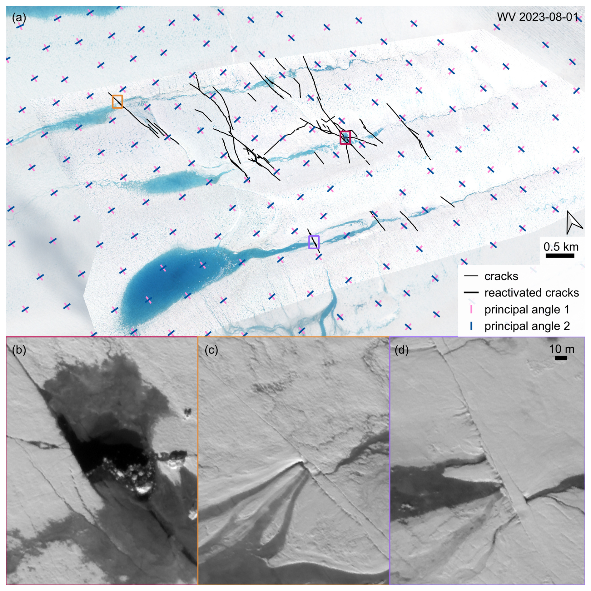
Figure 8 Detailed view of the 2023 drainage pathways. Panel (a) shows a WorldView multi-chromatic image (© DigitalGlobe, Inc. (2023), provided by European Space Imaging) from 1 August 2023 in the background, with black lines superimposed that denote crack locations. Fractures that already existed in 2022 are marked as bold lines, and new cracks formed in 2023 are shown as thin lines. The crosses denote principal stress directions retrieved from inverse modelling. Panels (b–d) display pan-chromatic imagery from the same acquisition as in panel (a) at locations marked in panel (a). The dark colour represents water.

3.2 Crack formation associated with drainage

Next, we present evidence of crack formation in accordance with lake drainage. As the drainage events in 2005/2006 and 2015 are different in type from the events from 2019 onwards, we start with these two events. In the events 2005/2006 and 2015, a long crack, transverse to the ice flow direction, appears over the entire width of the lake. A triangular-shaped feature is visible in both cases, with one side of the triangle located on the main long crack. A Pauli decomposition of the L-band ALOS-1 and ALOS-2 data reveals that the reflection is a double bounce, thus either from a crack face or a face of a higher-elevated block of ice. The triangular-shaped features also appear as double-bounce features.

The ALOS-1 quad-pol imagery from 3 April 2007 (Fig. 4a) reveals strong double-bounce reflectors. Among those reflectors is a linear feature with a triangular-shaped area, denoted as a line and a triangle in Fig. 4b. The same feature is also visible in a single-pol acquisition from 15 July 2006, and the distance equals the glacier motion. Its sides have a length of 200–300 m. No double-bounce reflectors are visible in an ALOS-1 quad-pol coverage on 4 November 2008 and 14 December 2010.

The long crack in the 2005/2006 event is shown in Fig. 4b. This crack can be followed over several years, although the appearance changes. The distance between the lines is not equal because satellite imagery is not available at the same time each year. Note that even in the (background) image from 2022, the 2005/2006 crack is visible as a shade. The shade indicates a vertical displacement of both crack faces, with the downstream side being elevated higher than the upstream side. This is also supported by the lake's shape after 2006, where a part of this crack marks the lake margin. Unfortunately, our database does not allow us to analyse if similar features also appeared in the 2012 drainage event.

A comparison of the drainage in 2005 and 2015 (Fig. 4b) shows that the triangular feature can be tracked over the years. In 2015, the crack is 2725 m long, and the triangle has a side length of 250–300 m. Both features are still clearly visible in the ALOS-2 imagery from 18 December 2016 as surface reflectors, 17 months after their formation. The high-resolution WV imagery from 2020 also shows a triangular-shaped feature of similar size (170–230 m side length); although strongly eroded, it is still identifiable in 2022, 7 years after its formation (Fig. 4). By 2021, the crack line visible in 2015 has disappeared, and the triangular feature is slightly off the trajectory between regions A and B, 200–500 m farther south. Most importantly, it now sits at a higher elevation, at the margin of the lake's middle branch, and is thus unlikely to be the main drainage channel.

We can identify the cracks associated with the drainage event based on the high-resolution imagery. Figure 8 shows the situation in 2023, and Fig. 9 shows an overview of 2019, 2020, 2022 and 2023. We find cracks in all three branches of the lake, but the densest network of cracks is situated in the middle branch, while the southern branch has only a few cracks in all the years. The crack system is centred around the triangular moulins. From there, cracks have reached in some years into the northern (2019, 2020, 2023) and southern (2019, 2022) branches. Wherever cracks are crossing river systems inside the lake area, it appears that water is flowing into the cracks (Fig. 8c and d), even weeks after the main drainage event occurred.

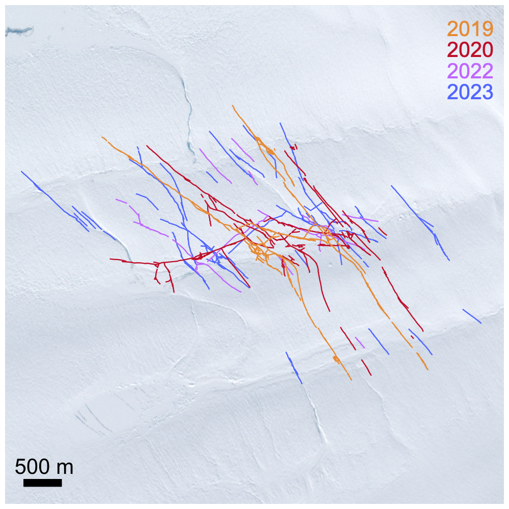
Figure 9 Cracks detected in the high-resolution optical imagery in 2019, 2020, 2022 and 2023. The background image is S2 on 5 September 2023.

The cracks predominantly match the principal stress directions (Fig. 8; calculated by inverse modelling, as in Humbert et al., 2023a), indicating that the dominant fracture mode is tensile (mode I). A close inspection of the surface of the lake ground shows that narrow and potentially shallow cracks exist in the area inside and outside the lake and also the presence of cracks that are not aligned with the principle direction (Fig. 8d). This is explained by the formation of tiny cracks at a 45° angle, which are formed in the main shear direction (similar to Humbert et al., 2023a). Once these cracks propagate at 45°, they form a connection from one row of narrow cracks to the next, where the crack propagation follows the main principal direction for a while until it again jumps onto the 45° and so on.

As the sun was low at one acquisition, we can use shadows to assess whether an uplift occurred across a rift. Figure 10 shows an inset around the drainage location with an arrow pointing to a shadow. We infer that an uplift has occurred along this crack and still exists 23 d after the drainage began. The conversion of shadow length to object height reveals the step between the crack faces to be roughly between 0.8 and 1.0 m (sun azimuth is 283.41° at acquisition, sun altitude 9.26° at 79.14360° N, 24.58510° W).

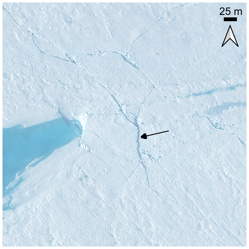
Figure 10 Triangular moulin fracture and cracks with uplift (WorldView image (© DigitalGlobe, Inc. (2019), provided by European Space Imaging) from 23 August 2019). The arrow points towards shadows that mark the uplift of the ice between the moulin and this crack.

3.3 Simulation of the conduit shape at the surface

To evaluate the shape and size stability of englacial channels, the model in Sect. 2.5.1 was set up. The deformation for a time span of 10 or 20 d is simulated to predict a tendency to open for an immediate drainage event. Figure 11 shows the resulting radial horizontal displacement on the hole boundary relative to the rigid body movement of 3.8 m d⁻¹ for three time steps. The shape of the curves t>0 indicates that the initially circular channel was deformed into an elliptical shape, with a mean change in radius of 0.032 m for t=20 d. The corresponding surface change is 0.3 %. From this, we conclude that our simulation predicts no significant surface change in the channel but a slight widening. This can be attributed to the different boundary conditions at the outer boundaries of the simulation domain. On the left side, we applied the upstream velocity of 3.8 m d⁻¹ and, on the right side, the downstream velocity of 3.9 m d⁻¹. Both velocities are in accordance with remote sensing observations. Because of the velocity difference, the simulation domain faces not only a rigid body motion but also an elongation, which appears to be a driving force for the opening of the channel in this model.

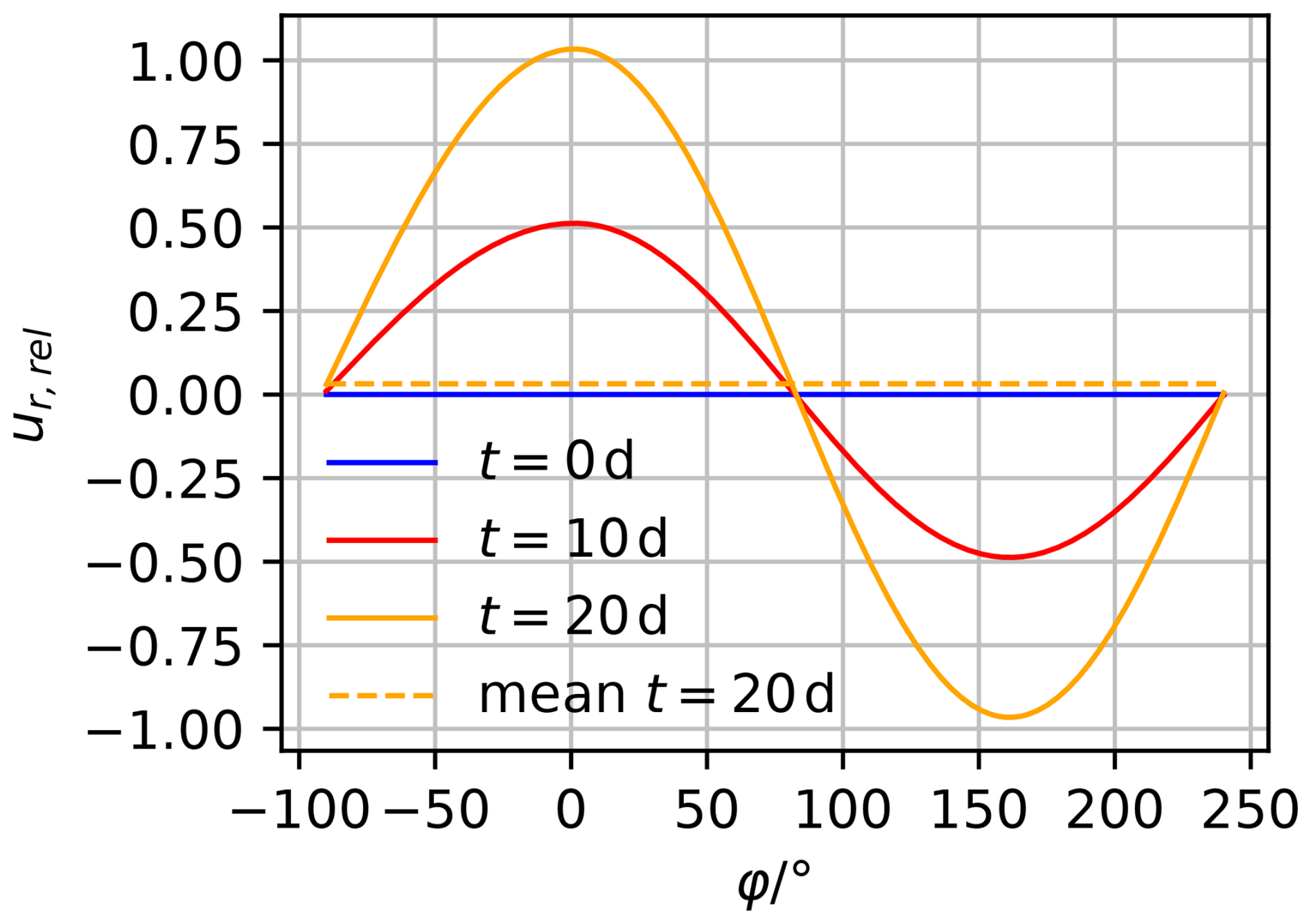
Figure 11 Simulated radial horizontal displacement of the hole boundary relative to rigid body movement.

3.4 Moulin refilling

We observed a refilling of the moulin at location B in the years 2020 and 2023. Figure 12 displays the satellite imagery in 2023 and 2020 in the upper and lower rows, respectively. After the main drainage event, we find an open moulin, where the darker pixels are shadows and the brighter pixels are sunlight reflections. On 31 July 2023, the moulin is filled with water, and a patch around the moulin is filled, too. In 2020, the scenario we observed was slightly different: within 4 d, the moulin overflowed. Some ice blocks were visible, and another 4 d later, it was empty again. Then, 16 d later, the drainage channel overflowed, and the area filled with water remained present until it froze. On 28 July 2020, the lake ground appeared wetter than the days before and after. This is not the case in 2023. In both years, cloud cover prevents a closer inspection; thus both the timeline and indications of the origin of the water need to be treated with care.

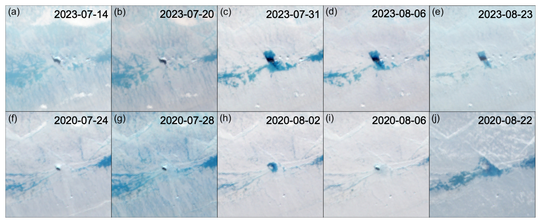
Figure 12 Refilling of the moulin after drainage from S2 images. The upper row (a–e) shows the temporal evolution in 2023, and the lower row (f–j) shows the temporal evolution in 2020.

3.5 Englacial features

Figure 13 presents three radargrams that are all acquired at the same flowline across the lake but in different years: 27 June 2016 (Fig. 13a), 11 April 2018 (Fig. 13b) and 29 July 2021 (Fig. 13c). Below the lake, the radargrams exhibit englacial reflections quite distinct from normal stratigraphic internal layering or folds near the base. No englacial reflections are found near the lake downstream of the presented profile. Please note that with our flight profile, we are likely crossing a three-dimensional feature, while we do not have any information of the perpendicular direction.

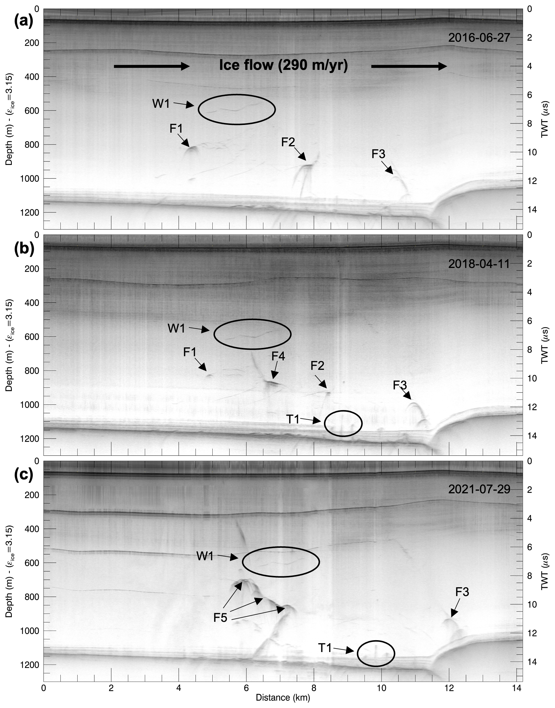
Figure 13 Radargrams along the cross-section in the along-flow direction of the glacier (red line in Fig. 1) acquired in 2016 (panel a), 2018 (panel b) and 2021 (panel c). All three radargrams show the same cross-section. The flow direction of the glacier is from left to right. The location of the transects is shown in Fig. 1. We identified englacial features (labelled F1 to F5), which reoccur in all three panels (F3) or are newly developed (F4, F5). A persistent wing-shaped feature is labelled W1, and a triplet of features close to the ice bed are labelled T1.

We find in 2016 three prominent features 200–300 m above the ice base (at distances of 4.5, 7.8 and 10.5 km, denoted as F1, F2 and F3 in Fig. 13a). There are further features visible that appear as thin, oblique or wing-shaped reflections with lower amplitude (at distances of 3 to 7.5 km), of which the one closest to the ice surface (lake base) is at a depth of roughly 500 m (W1 in Fig. 13a). In 2018, all three prominent features (F1–F3) are still present. Features F1 and F2 have changed their width and strength; they have become narrower and have a lower amplitude than in 2016. One new prominent feature appeared at a distance of about 6.8 km (denoted as F4 in Fig. 13b) and is located about 300 m above the bed.

In the radargram from 2021 (Fig. 13c), the uppermost englacial feature is only 300 m below the lake ground. It is the only profile containing reflections high up in the ice column. A wide feature is visible at a 5.5–7.5 km distance, consisting of several individual hyperbolas (denoted as F5 in Fig. 13c). Above and below we find two smeared or diffuse reflections: one from about 250 m below the lake ground, pointing towards feature F5, and one in the lower 250 m, oriented towards the base.

One of the less strong reflections (W1) from 2016 can be found with a strikingly similar shape in the radargram from 2018 and 2021, located at a position approx. 1 km downstream, which is consistent with the surface velocity of the glacier. A triplet of features close to the ice base in the radargram of 2018 (T1) is visible in the 2021 radargram in the same shape, just advected downstream.

The feature farthest downstream (F3 in Fig. 13a) can be tracked over the 5 years. As in the other cases, its travel distance corresponds to the glacier's velocity. Interestingly, in 2021, it is smeared out, which could potentially originate from vertical shear while climbing across the bedrock step. Using the glacier velocity to trace this feature upstream shows that it would have been located in 2005 at location A. Thus, it may be the remnants of the first drainage event.

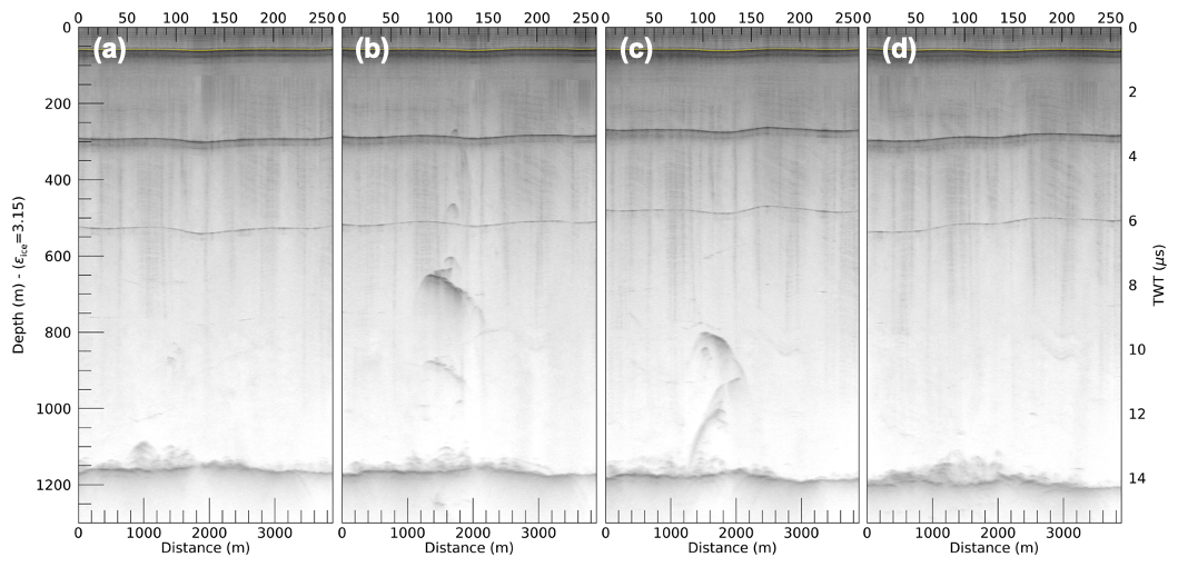
In 2021, we acquired four transects across the flow direction and the along-flow direction profile. Their position is shown in Fig. 1a. The across-flow profile acquired farthest upstream is acquired at the location of the moulin fracture in region A in 2020 (not at the location where the moulin fracture advected to at the time of the airborne survey). It exhibits some englacial features in the lower 100 m (Fig. 14a). The second one is recorded 380 m downstream of the moulin fracture at location A. This radargram contains strong englacial reflections, which are located about 500 m above the base (Fig. 14b). The lateral extent of these englacial features is 1 km. Farther up in the ice column, a narrow feature is found, which is located 400 m below the ice surface (lake ground). Very close to the base, several hyperbolas are visible. The third across-flow profile is located just 150 m upstream of the moulin fracture from the 2020 event, at location B. We again find a strong internal reflector, situated about 300–400 m above the base, and a lateral dimension of 1 km (Fig. 14c). Below this reflector, we also find hyperbolas close to the base. The fourth cross-section within the lake area is 1.2 km downstream of the moulin at location B. This radargram exhibits no strong englacial feature but has a broader and higher area of hyperbolas close to the base (Fig. 14d).

Figure 14 Radargrams in the across-flow direction from the upstream end of the lake to the downstream end. The location of the transects is shown in Fig. 1.

3.6 Blister evolution

These radargrams give some insight into englacial drainage pathways, so now we must consider where water masses might be stored beneath the glacier and how this varies in time. We use double-differential interferometry data from 2019 to assess the evolution of the surface elevation after the drainage event. Unfortunately, the surface condition allows this to occur only 3 weeks after the drainage. Figure 15 displays the displacement from 3–4 to 7–8 weeks after the main drainage, and Fig. B1 shows the interferograms. The results are discussed with respect to the absolute displacement and its location relative to the lake area and cracks. The centre of the fringes is at the beginning slightly upstream of the moulin fracture location. The largest displacement occurred directly in the lake. Still, it reaches about 2.3 km in the downstream direction, 2.0 km in the upstream direction and even ∼6 km in the northward direction (going beyond the neighbouring lake). The downstream end of the fringes coincides with the bedrock step visible in Fig. 13, at a distance of 11.5 km. In the subsequent weeks, this extent reduces, and the centre of the fringes moves slightly downstream to the moulin fracture. The magnitude outside the lake is significantly lower and, in the order of magnitude, this is consistent with the vertical displacement detected by the GNSS stations (see Fig. A1). During the time covered by the interferogram, the level of the remaining water patches does not change anymore. Still, lake ice is formed, which is not covered by a snow layer (last optical imagery from 7 September 2019). This indicates that the elevation change is due to a blister formed during the drainage underneath the lake.

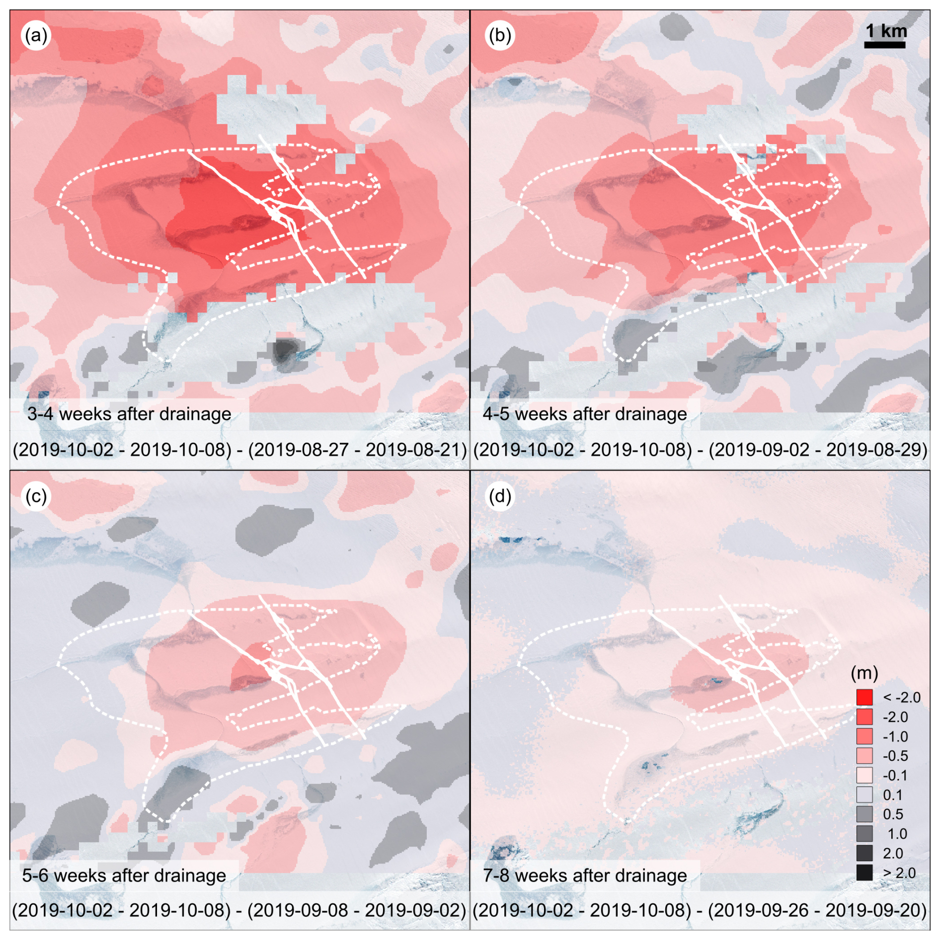
Figure 15 Surface elevation change based on interferograms, with the red colour representing subsidence. The four panels cover 3–4 to 7–8 weeks after the main drainage. The dashed white line represents the maximum filling on 26 July 2019, while the bold white line represents the cracks on 23 August 2019. The background image is an S2 image from 7 September 2019.

3.7 Atmospheric forcing

As a last step, we want to set all previous results in the context of atmospheric forcing, the origin of lake genesis and subsequent processes. We present skin temperatures in the lake's catchment from the 1990s to 2022 in Fig. 16. Each year is shown as a grey line, while 5-year median skin temperatures are superimposed in colour (the first and last average contain fewer years). While the median shows little variation in magnitude in mid-July, early and late summer temperatures have increased substantially. This increases the period in which melt occurs and, consequently, the amount of meltwater available. Below, we will synthesise this dataset with lake filling and drainage observations.

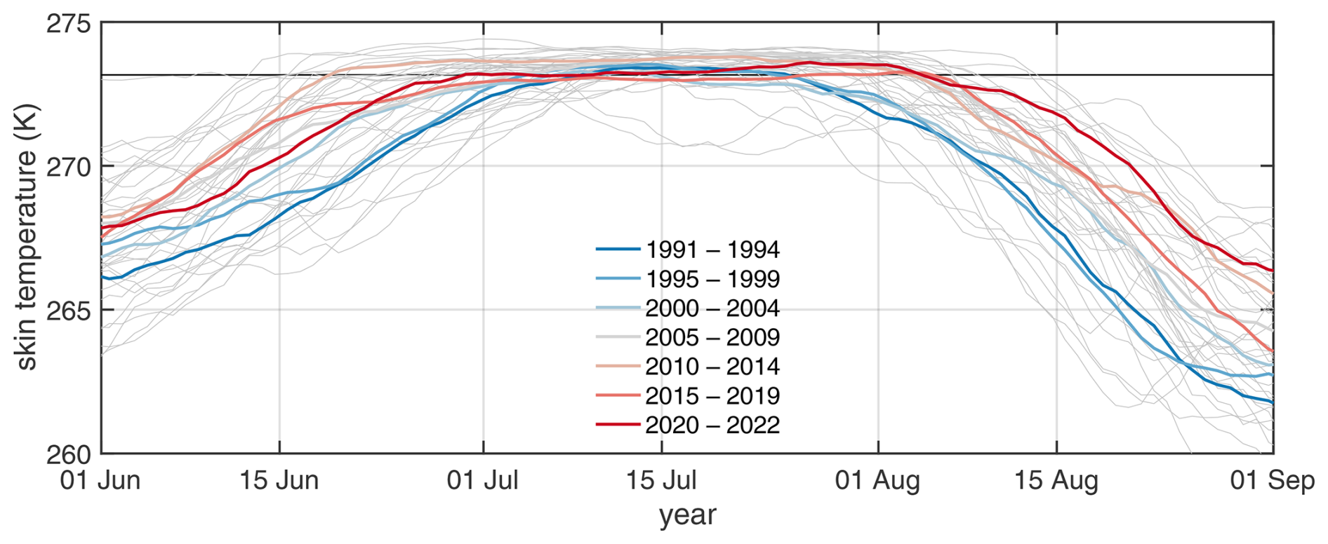
Figure 16 Atmospheric forcing: CARRA skin temperatures from the 1990s to the present. Each year is displayed in grey, and the median temperatures of 5 years (the first and last periods are shorter) are superimposed in colour.

4 Discussion

We begin our discussion with an evaluation of the evolution of the lake, followed by an analysis of the surface and englacial fractures, before attempting to understand their long-term change and the climate context.

After the genesis of the lake, its size was reduced over time. With the occurrence of triangular moulin fractures from 2019 onwards and more frequent drainages, the size of the lake remained diminished. We suggest that this is due to the reactivation of former moulins for which we expect a lower mechanical load to be required than for the formation of entirely new fractures. The reactivation is feasible because the lake length is large compared to the glacier motion per year. The fractures are for a long time in the topographic low and, with that, also in the area of highest water pressure at the lake bed.

The triangular moulin fractures and further cracks are concentrated around two locations (marked A and B in Fig. 1). One potential reason for this is the influence of bed topography on the local stress field. The coincidence of moulin location with bedrock ridge was found by Catania and Neumann (2010). To clarify this further, a dense coverage of radar survey flights over this lake is required, which is highly recommended for future airborne campaigns. We find crack formation with lake drainage near the triangular moulin fracture at location B. We envisage the drainage to occur not only through the large triangular pathway but also through these cracks, similar to the studies of Das et al. (2008) and Chudley et al. (2019). In the optical imagery after drainage, the cracks are very narrow, and we assume they closed (not healed) elastically after the water passage. The radargrams (Figs. 13 and 14) intersect a network of cracks and englacial channels. Although we know the fractures only at those intersections, the multitude of reflections demonstrate that more than only one pathway for water exists. Therefore, we anticipate that elastic contributions in fracture closure and blister formation are essential, and a more complete fracture mechanical analysis is needed, ideally a combination of airborne radar surveys and in situ measurement networks such as in Chudley et al. (2019), combined and repeated over multiple years.

The radargram in 2016 was acquired 11 (and 47) months after lake drainage. In 2018, no massive drainage occurred before data acquisition. The profile in 2021 was measured 12 and 24 months after enormous lake drainage. Thus, we do not measure right after a moulin fracture or surrounding cracks are formed, which limits the interpretation of the radargrams slightly: in particular, the assignment of a radargram feature to a surface feature. On the other hand, only the survey long after the drainage events enables us to assess the long-term englacial changes. Both come with pros and cons.

The prominent features we see in the radargrams are all within 850 m above ground. Our radar is not sensitive in the uppermost tens of metres of the ice sheet in this setting; thus we cannot measure any features right below the lake ground. Nevertheless, it is consistent for all three acquisitions that the upper 200 m of the ice is free of englacial features almost a year after the drainage events. Features within 850 m above ground are either changing over time (features indicated by F1 and F2 in Fig. 13) or remaining nearly similar while being advected with the ice flow (features indicated by W1, T1 and F3 in Fig. 13). This could be related to a hydraulic head of 850 m above the ground, which would exert some pressure that counterbalances creep shut. We find no change in the size and geometry of the triangular moulin between 2020 and 2022. At the end of summer 2020 and 2023, the hydraulic head at the moulin is still above the lake ground (see Fig. 12). This shows an increase in the head due to the drainage compared to the “background” hydrological system without any perturbation due to lake drainage.

Interestingly enough, several internal features situated in the lower half of the glacier (W1 in Fig. 13), even very close to the bottom (T1 in Fig. 13), move without any change in shape or appearance. This indicates a plug flow regime and no healing during our observational period. Assuming that the farthest downstream feature is indeed from 2012, we infer that even after 9 years, no healing took place. On the other hand, we do find that the most prominent features from 2016 (F1 and F2 in Fig. 13) changed their shape by 2018 and 2021. The first drainage event in 2005/2006 was located farther south than the profile we surveyed here, which is potentially the reason why we do not see any features that can be linked to this event in the radargrams.

We find evidence for the reactivation of former drainage pathways. This would fit well with the finding that the triangular moulin and fractures are not forming at the same geographical location in every drainage year but that the positions fit the advection with the glacier motion. The temporal evolution of the reactivation was in all but one case during our observational period, such that the englacial part of the moulin must have been shut, allowing the lake to fill, as the former moulin fracture is visible at the lake ground before the drainage was triggered. We find that the triangular moulin was reactivated with the subsequent drainage, but more fractures in the vicinity were formed. In one case, the reactivation was different: the lake did not fill in 2021, which suggests that the moulin from 2020 was still active, and water was continuously flowing into the moulin fractures that summer. Also, the velocity increase of 10 % in summer 2017 (Fig. A1) indicates higher bed lubrication, consistent with a decline in the water body in the satellite imagery. This points to a still-active drainage system. In both cases, an easy-to-reactivate system is conceivable but cannot be distinguished here from a still-active system. We also found deactivated former drainage pathways: a crack in 2019 downstream of the moulin was active in 2015's drainage but inactive in 2019.

We found ice blocks that became afloat (Fig. 6) and drifted some distance from their origin before drainage. This indicates a succession of events before the large cracks and englacial fractures facilitate the drainage. What controls the size of these blocks is so far unclear. We find that the ice blocks from 2022 are, before and after the drainage in 2023, still in the same constellation, which indicates that they did not become afloat again, and no drift took place. We envisage the following reason: the water level at the end of 2022 was low enough that it froze entirely during winter, encapsulating the blocks. This may also have led to a more rapid filling of the lake, as less water volume is needed to reach the same area extent than in other years.

The principal stresses mainly control the fracture orientation at the surface, and fractures mainly appear as mode I cracks, with some deviations due to shear-dominated crack tips. The repeated formation of fractures that lead to a triangular shape for the main drainage channel is not easy to understand from the observations and will need some fracture mechanical modelling studies. The GNSS data from 2019 also reveal that the drainage started after the seasonal acceleration. This could act as a drainage event trigger if the stresses are already close to a critical threshold, as an increase in strain rate acts as an additional displacement boundary condition, as suggested by Alley et al. (2005).

Prominently, the vertical displacement between the crack faces remains longer (Fig. 4). This has also been observed by Doyle et al. (2013). The high-resolution imagery is all taken a couple of weeks after the drainage event (and thus in the phase where the blister is relaxing), and still, rivers flow into the cracks, supplying the basal system with further water volume. This implies that the hydraulic head is below the glacier surface in some years. In contrast, we find a refilling of two moulins (Fig. 12) in 2 years, which implies that the hydraulic head is at or above the glacier surface. Chudley et al. (2019) have found considerable uplift downstream of the lake after drainage, while in our case, the largest vertical displacement is inside the lake area (based on subsidence weeks after the drainage; Fig. 15).

We have so far discussed the mechanisms involved in lake drainage and their impact in detail. We now want to take a broader perspective: with the surface temperature increase in the mid-1990s (Fig. 16), the lake started to form (Table 2). In just 10 years, this subglacial hydrological system changed from no seasonality to seasonality and extreme events in the form of massive and abrupt perturbations of meltwater input timescales of hours to days. These are extreme perturbations of a system, and it is still not explored how the ability of the englacial and subglacial system to receive this water amount influences the drainage itself.

A crucial question is if the frequent drainage events have forced the system into a transition of a new state or if the system is (still) getting back to a normal winter state despite such extreme water inputs. Farther downstream of this lake, massive changes in the system occurred, in which 500 m high channels at the underside of the ice developed (Zeising et al., 2024). After 2015 – the year with the highest lake volume – the channel evolution increased significantly. As the channel is on the grounded ice, its formation has to be driven by subglacial discharge. It is plausible that the lake evolution we presented here and the frequent drainages in the past years contributed to the formation of the channel. The imminent question is how this system will evolve in future.

5 Conclusions

This study is concerned with a massive supraglacial lake at 79NG, formed only in the mid-1990s. We find that the formation of this lake is linked to an increase in surface temperature in the lake's catchment. The lake volume exceeded 10⁸ m³ in 2015, but after that, the reactivation of drainage pathways led to smaller lake volumes, and drainage happened more frequently. The drainage pathways are cracks and triangular-shaped moulins, which can become water-filled in some years when the hydraulic head rises to exceptionally high values, a condition that persists until freezing. The cracks cause the vertical displacement of ice that remains detectable more than 15 years after the initial drainage. Englacial features also persist directly underneath the lake or are advected downstream with a slightly altered shape. We find a blister beneath the lake and its neighbourhood of non-radial shape that relaxes over 2 months. The multitude of observational methods enabled us to obtain an understanding of the genesis of supraglacial lakes, from inexistence to frequent drainage. This type of approach can provide useful insights for developing models from fracturing, englacial pathway formation and closure, and the response of the subglacial system.

Appendix A: GNSS

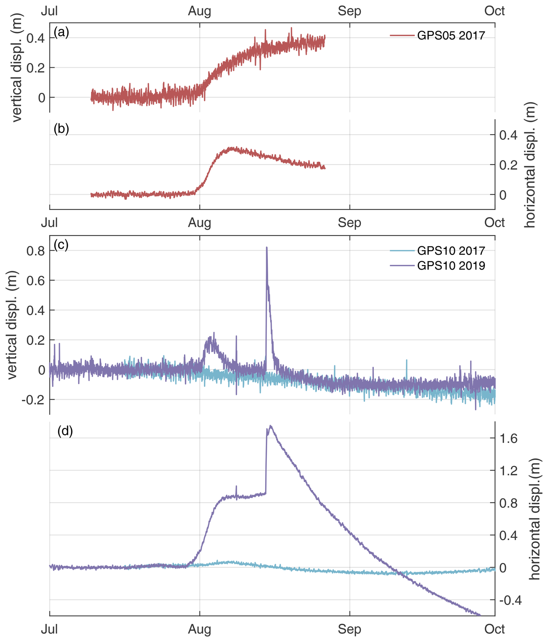
Figure A1 Horizontal and vertical motion in the vicinity of the lake. Panels (a) and (b) present data from a GNSS downstream of the lake in the summer of 2017, while panels (c) and (d) display data about 5 km distance to the lake in the summer of 2017 and 2019. The location of the GNSS stations is shown in Fig. 1.

Appendix B: Blister relaxation

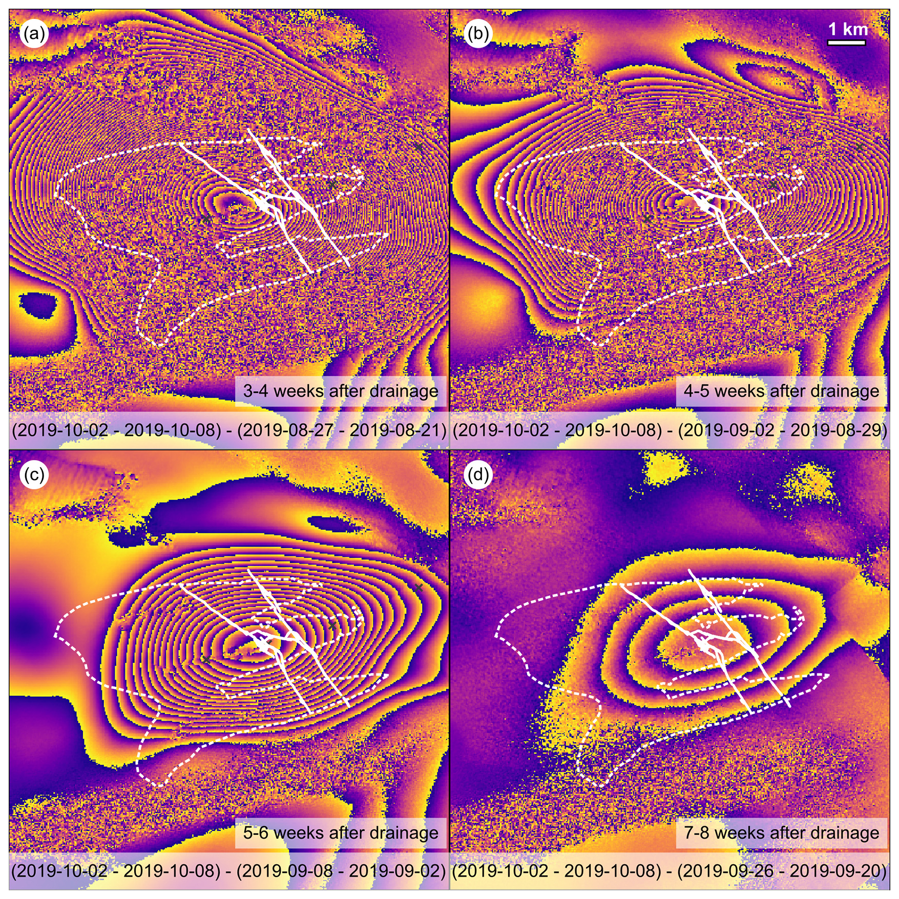
Figure B1 Double-differential interferograms using Sentinel-1 data. The four panels cover 3–4 to 7–8 weeks after the main drainage. The dashed white line represents the maximum filling on 26 July 2019, while the bold white line represents the cracks on 23 August 2019.