Sea level rise contribution from Ryder Glacier in northern Greenland varies by an order of magnitude by 2300 depending on future emissions

The northern sector of the Greenland Ice Sheet contains some of the ice sheet's last remaining glaciers with floating ice tongues. One of these glaciers is Ryder Glacier, which has been relatively stable in recent decades, in contrast to the neighbouring Petermann and C.H. Ostenfeld glaciers. Understanding Ryder Glacier's future behaviour is important as ice-tongue loss could lead to acceleration and increased ice discharge. Meanwhile, it is unclear whether Greenland-wide modelling attempts are able to accurately resolve the influence of fjord and bedrock topography and small-scale variations in ice dynamics for a glacier like Ryder. To fill these gaps, here we conduct targeted high-resolution modelling of Ryder Glacier until the year 2300. We find that mass loss is dominated by discharge under a low-emissions scenario all the way to 2300, leading to a sea level contribution of between 0.8 and 2 mm depending on the amount of ocean warming. Discharge also plays a key role under a high-emissions scenario up until 2100, after which a strongly negative surface mass balance becomes the dominant driver of mass loss. This negative surface mass balance leads to a much higher sea level rise contribution by 2300 of between 44 and 52 mm, with little sensitivity to the range of ocean warming scenarios used in this study.

1 Introduction

The Greenland Ice Sheet is currently the largest single contributor to global sea level rise, having exhibited an acceleration of mass loss during the last 2 decades (Briner et al., 2020; King et al., 2020; Millan et al., 2023; Greene et al., 2024). Mass loss occurs both due to a negative surface mass balance and through dynamic loss directly into the oceans – with these dynamic processes having driven the recent increase in mass loss (King et al., 2020). Air temperatures in northern Greenland are already higher than at any time during the past millennium (Hörhold et al., 2023), and current projections suggest we are on track to experience rates of mass loss that have not been seen during the entire Holocene (Briner et al., 2020; Goelzer et al., 2020). Paleo-evidence suggests that the Greenland Ice Sheet as a whole is sensitive to substantial deglaciation in climates that are only slightly warmer than at present (Schaefer et al., 2016) and that a rise in global mean temperatures of around 2°C above pre-industrial temperatures may be enough to trigger self-sustained melting of the Greenland Ice Sheet (Bochow et al., 2023). However, the large degree of spatial heterogeneity in Greenland outlet glacier behaviour contributes to a large uncertainty in the response of these glaciers to ocean forcing (Mouginot et al., 2019).

The northern sector of the Greenland Ice Sheet has been relatively understudied (Hill et al., 2018b), and uncertainties with respect to the future behaviour of this region are considered larger than for other sectors of the ice sheet (Choi et al., 2021; Goelzer et al., 2020). One reason for this is that this sector contains the last few remaining ice tongues in Greenland (Millan et al., 2023). If these floating ice tongues are lost, the reduction in buttressing has the potential to accelerate upstream ice flow and associated dynamic mass loss (Millan et al., 2023). In total, this sector has the potential to contribute ca. 93 cm to global sea level rise (Mouginot et al., 2019), with the associated increased freshwater release to the oceans having knock-on impacts through changes in biogeochemical conditions (Kanna et al., 2022) and through potential weakening of the Atlantic Meridional Overturning Circulation (Yang et al., 2016).

Observational records from recent decades have shown a large degree of spatial heterogeneity between neighbouring glaciers, underscoring the high uncertainty surrounding the future behaviour of glaciers (Porter et al., 2014, 2018; Cooper et al., 2022). As such, recent research has concluded that changes need to be considered at the scale of individual glaciers (Cooper et al., 2022) and that seemingly stable glaciers are key targets for ongoing research due to the potential for rapid retreat to occur out of sync with climate forcing (Robel et al., 2022). Heterogeneity in glacier behaviour is well exemplified by considering three northern Greenlandic glaciers: the Petermann, Ryder, and C.H. Ostenfeld glaciers. The Petermann and Ryder glaciers are two of the few Greenlandic glaciers which still have a floating ice tongue, although Ryder Glacier also has a smaller, grounded terminus. Petermann Glacier has been retreating, having lost around 40 % of its ice tongue over the past 15 years (Münchow et al., 2016), whilst Ryder Glacier's terminus position has shown little net movement. Petermann Glacier exhibited an average terminus retreat rate of 311 m yr⁻¹ between 1948 and 2015, at the same time as Ryder Glacier experienced little overall change in margin position despite periods of both advance and retreat (Hill et al., 2018b; Holmes et al., 2021). Meanwhile, C.H. Ostenfeld Glacier lost its ca. 20 km long ice tongue between 2002 and 2003 and has since had a relatively stable front position (Hill et al., 2018b). It has previously been suggested that a shallow bathymetric sill in front of Ryder Glacier's grounding line may be responsible for the lack of terminus and grounding line retreat through blocking intrusions of warm Atlantic water, thus keeping melt rates under the ice tongue low (Jakobsson et al., 2020; Nilsson et al., 2023). This is in contrast to Petermann Glacier, which has a bathymetric sill with a deeper channel that has been shown to allow greater intrusion of warm Atlantic water (Jakobsson et al., 2018). Although this likely goes some way to explaining Ryder Glacier's terminus stability, uncertainties remain in light of the fact that recent satellite-derived observations of ice-tongue melt at the Petermann and Ryder glaciers have indicated significantly higher grounding line melt rates at Ryder Glacier than at Petermann Glacier during the 2000–2020 period (Millan et al., 2023).

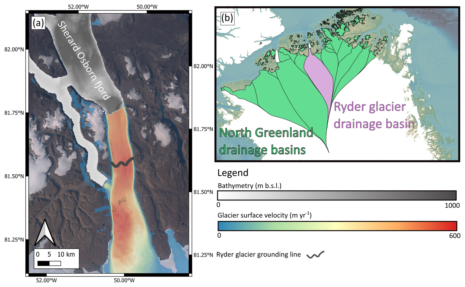
Figure 1 Close-up of the frontal area of Ryder Glacier (a), with the position of its drainage basin in northern Greenland shown (b). The present-day velocities, grounding line position, and fjord bathymetry are shown. Drainage basins are from Mouginot et al. (2019). The bathymetry and grounding line position are from BedMachine v5 (Morlighem et al., 2017). The satellite image is a 2019 Sentinel-2 image mosaic from MacGregor et al. (2020). The surface velocities are from 2015–2016 and were obtained from the MEaSUREs dataset (Joughin et al., 2016, 2018).

Looking towards the future, several studies have identified the need to understand the dynamic impact of ice-tongue loss in northern Greenland and the potential impact on sea level rise projections (Millan et al., 2018; Hill et al., 2018b; Millan et al., 2023). Specifically, there is a possibility for discharge to increase substantially after the breakup of an ice tongue due to the loss of buttressing. This behaviour is however complex and varies from glacier to glacier, making its incorporation in future projections an area of uncertainty. This is of particular importance in the present day as recent observations have suggested that all of Greenland's ice tongues have experienced considerable weakening during the last few decades (Millan et al., 2023). Whilst there have been many targeted studies of Petermann Glacier (Nick et al., 2012; Hill et al., 2018a; Rückamp et al., 2019; Åkesson et al., 2022) and analysis of C.H. Ostenfeld Glacier's response to ice-tongue collapse (Hill et al., 2018b), we are not aware of any published studies focusing on Ryder Glacier and how it may respond to future ice-tongue collapse. Whilst several studies have targeted the future behaviour and sea level rise contribution from the entire Greenland Ice Sheet, the associated computational cost means that the spatial resolution of these models is often relatively coarse, and processes such as ice–ocean interactions are crudely represented (Aschwanden et al., 2019; Beckmann and Winkelmann, 2023; Choi et al., 2021). These considerations lead to two key research questions. (i) How will Ryder Glacier respond to future climate change, and what are the implications for sea level rise? (ii) How does potential future ice-tongue loss at Ryder Glacier compare to neighbouring systems in northern Greenland, and what does this tell us about the controls on ice-tongue and glacier evolution?

To answer these questions, we conduct targeted, high-resolution simulations of Ryder Glacier's response to future projected atmospheric and oceanic changes. Ryder Glacier is of particular interest in light of the fact that it has not been retreating in recent decades and, unlike Petermann Glacier, has not previously been the focus of targeted modelling studies. By disentangling the controls on glacier evolution under different magnitudes of climate warming, the results from our simulations will have implications for other glacier–fjord systems. The background on the numerical model is given below, followed by a description and discussion of the model results.

2 Methods

The numerical model employed in this work is the Ice-sheet and Sea-level System Model (ISSM) (Larour et al., 2012), a finite-element model that has been used extensively to model glaciers in both Greenland and Antarctica.

The model domain encompasses the entire drainage basin of Ryder Glacier, as defined by Mouginot et al. (2019), and is shown in Fig. 1. It is extended up until the mouth of Sherard Osborn Fjord to allow for potential glacier advance during all relaxation and forward simulations. The mesh is extruded to have seven vertical layers, and the horizontal mesh resolution varies between 300 and 10 000 m based on surface velocity, with areas flowing faster than 500 m yr⁻¹ having the finest resolution. For the bathymetry and bedrock topography, we use BedMachine v5 (Morlighem et al., 2017), which includes the newest bathymetric data from the Ryder 2019 expedition to Sherard Osborn Fjord with the Swedish icebreaker Oden (Jakobsson et al., 2020). For the initial surface elevation, we use the GIMP DEM with a nominal date of 2007 (Howat et al., 2014), which is provided along with BedMachine v5 (Morlighem et al., 2017).

For all simulations, a higher-order (HO) approximation of ice flow, the Blatter–Pattyn approximation, was used, which is computationally cheaper than full-Stokes approximations (Blatter, 1995; Pattyn, 2003). Previous studies have compared this HO approximation to full-Stokes set-ups and found limited differences, with the velocity–thickness misfit between HO and full-Stokes solutions being smaller than that between the full-Stokes solution and the even cheaper shelfy-stream approximation (Yu et al., 2018). For transient simulations, the time step size was set to 0.083 years, corresponding to a monthly time step. In scenarios where large accelerations were observed, the simulations were re-run with a time step of 3 d (0.008 years) in order to satisfy the Courant–Friedrichs–Lewy condition (Courant et al., 1928).

2.1 Model set-up

The first step in the workflow was to invert for basal friction under glaciated areas by minimising the misfit between modelled velocities and observed 250 m resolution velocities in 1995–2015 from MEaSUREs (Joughin et al., 2016, 2018).

For all simulations, a Budd-type friction law is used. This law was found through a comprehensive comparison of several friction laws to work best for the neighbouring Petermann Glacier (Åkesson et al., 2021). This friction law has additionally been used successfully for simulations covering the entire Greenland Ice Sheet (Choi et al., 2021). Here, basal drag τ_b is based on the inverted friction parameter α, basal velocity u_b, and effective pressure N, which itself is calculated from ice density ρ_i, water density ρ_w, gravitational acceleration g, ice thickness H, and ice base elevation b, as follows:

$$\begin{array}{}\text{(1)}& {\mathit{\tau }}_{\mathrm{b}}=-{\mathit{\alpha }}^{\mathrm{2}}N{\mathit{u}}_{\mathrm{b}},N={\mathit{\rho }}_{\mathrm{i}}gH-{\mathit{\rho }}_{\mathrm{w}}gb.\end{array}$$

Similar to several recent studies, an inversion was also performed to infer the spatially variable rheology of the floating ice tongue, using the same velocity dataset that was used to infer the friction parameter α under grounded ice (Åkesson et al., 2021; Choi et al., 2021; Åkesson et al., 2022; Humbert et al., 2023; Wilner et al., 2023). The rest of the domain is assumed to have a constant viscosity matching the behaviour of an ice temperature of −12 °C based on the ISMIP6 Greenland experiments (Goelzer et al., 2020).

Basal melting below the ice tongue is prescribed so that it varies linearly with depth in a manner that is consistent with observations from northern Greenland (Slater and Straneo, 2022). Here, basal melt is initially set to equal 0 m yr⁻¹ at depths shallower than 100 m and linearly increases to a maximum melt rate of 40 m yr⁻¹ for depths at or below 300 m. These values are based on observations of Ryder Glacier from Wilson et al. (2017), where melt rates of ca. 40 m yr⁻¹ are found at the grounding line, decreasing to ca. 0 m yr⁻¹ as the ice tongue thins towards the terminus. Observations additionally show considerable lateral variation in grounding line melt rates (e.g. between 10 and 60 m yr⁻¹) – something that is not accounted for here. In all simulations, including the relaxation, the melt rate applied across the entire submarine portion of any grounded part of the terminus is set to equal half of the maximum melt rate below the floating tongue – something that was chosen due to the fact that it allowed for a stable terminus during the relaxation and required no inputs of e.g. temperature or subglacial discharge for calculations, as these data points are not available for this part of the fjord. This, for example, applies to the smaller grounded calving front that Ryder Glacier has in the present day.

Calving is another important mass loss process at Ryder Glacier's marine margin, with the choice of the calving law being identified as a key source of uncertainty in models of Greenland's future (Goelzer et al., 2020). We use a von Mises calving law for all simulations, chosen as recent studies comparing several different calving laws found it to perform best in both Greenland and Antarctica (Choi et al., 2018; Wilner et al., 2023). The von Mises calving law computes the calving rate c depending on the terminus velocity u and the von Mises tensile stress $\stackrel{\mathrm{̃}}{\mathit{\sigma }}$ (Morlighem et al., 2016). In this formulation, calving occurs where the von Mises tensile stress is greater than the tuned stress threshold parameter σ_max.

$$\begin{array}{}\text{(2)}& c=\left|\mathit{u}\right|{\displaystyle \frac{\stackrel{\mathrm{̃}}{\mathit{\sigma }}}{{\mathit{\sigma }}_{max}}}\end{array}$$

The stress threshold σ_max is set to 200 KPa for floating ice and 500 KPa for grounded ice (see Sect. 2.2 for information on how this was chosen).

Atmospheric-driven forcing is also included in all simulations through the use of surface mass balance (SMB) datasets. Several different reference datasets are used in this study, with all of them being outputs from CESM2-forced RACMOv2.3p2 simulations at a 1 km resolution. To improve the representation of SMB as the ice elevation changes with time, we set a relation between surface elevation and SMB to account for the melt–elevation feedback, which is often neglected in similar studies (Nick et al., 2013; Bassis et al., 2017; Steiger et al., 2018). This is incorporated through the use of the SMB gradient module implemented in ISSM, where the SMB from a reference dataset is altered at each time step to account for changes in surface elevation (Helsen et al., 2012). The gradient method is only applied in the ablation zone (evaluated at each time step based on where the reference dataset shows a negative SMB) due to uncertainties regarding the melt–elevation relationship in the accumulation zone (Helsen et al., 2012; Calov et al., 2018; Choi et al., 2018).

2.2 Model relaxation

Before running the forward simulations which constitute the results of this study, a relaxation simulation is run for 50 years with two main aims: (i) to calibrate the calving parameters (see Eq. 2) and (ii) to validate the model against present-day observations of Ryder Glacier and trends at Ryder Glacier since 2000 (Fig. 2). Specifically, we compare the relaxed state of the model to mean 1995–2015 velocities (Joughin et al., 2016, 2018), present-day thicknesses from BedMachine v5 (Morlighem et al., 2017), the trend of mass loss since 2000 (Mouginot et al., 2019), front position changes since 2000 (Holmes et al., 2021), and grounding line position changes since 2000 (Millan et al., 2023).

Both SMB and basal/frontal melt were applied during the relaxation. We use a temporally fixed SMB forcing equal to the mean of 1950–2014 SMB from RACMO (Noël et al., 2022a). Basal melt follows a linear increase with depth described in Sect. 2.1, with the maximum melt rate kept constant at 40 m yr⁻¹. The calving stress threshold σ_max for both floating and calving ice is calibrated by running this relaxation with various values for each parameter to find the best fit, beginning with the values used by Åkesson et al. (2021) for Petermann Glacier and then adjusting by 20 KPa with each iteration in response to whether too much advance or retreat was seen. As was done by Choi et al. (2018), we compare the overall terminus position change when choosing the calibration parameters – e.g. we chose the values of σ_max that led to a stable terminus position rather than trying to recreate the cycles of advance and retreat that have been observed at Ryder Glacier. This is because the chosen calving law is a calving rate law – i.e. it does not model individual calving events but the overall advection of the front. Whilst this means that it does not always perfectly recreate the pattern of ice front migration (such as the cyclic advance and retreat at Ryder Glacier), it performs well over the centennial cycles we aim to simulate in this study (Choi et al., 2018).

During the 50-year relaxation simulation, Ryder Glacier exhibits mass loss equal to 0.9 Gt yr⁻¹, which is similar to the observed mass loss between 2000 and 2017 of 0.96 Gt yr⁻¹ (Mouginot et al., 2019). The front position remains stable throughout the relaxation, corresponding with reports of net terminus stability at Ryder Glacier (Holmes et al., 2021). A small grounding line retreat of ca. 2 km is seen in the relaxation – something which corresponds to recent reports of Ryder Glacier's behaviour (Millan et al., 2023). Modelled velocities and thicknesses at the end of the relaxation match well with observed velocities, with ice-tongue speeds of around 550 m yr⁻¹. The velocities, thicknesses, terminus movement, and grounding line movement from the relaxation in comparison to observations are shown in Fig. 2.

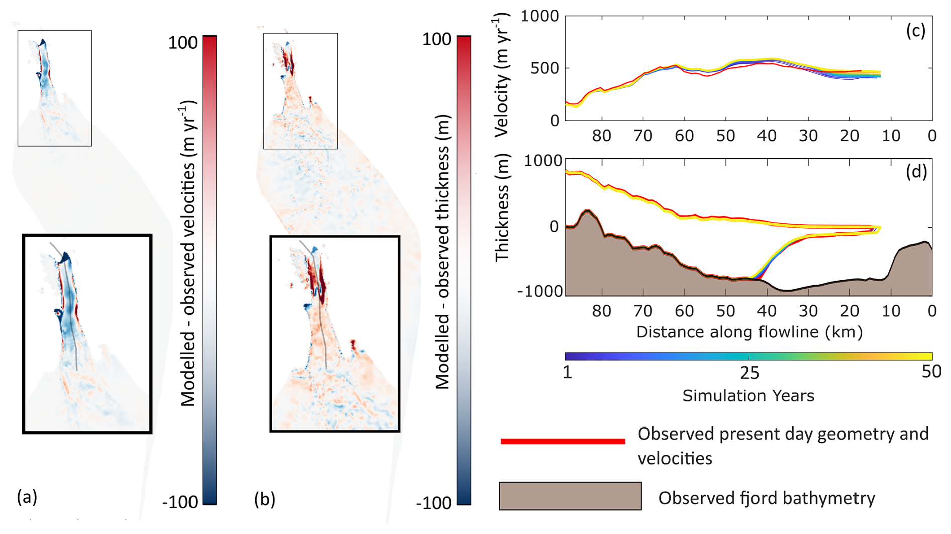
Figure 2 Modelled state of Ryder Glacier at the end of the relaxation. The misfit between the modelled and observed velocities is shown in (a), alongside the thickness misfits in (b), with a inset close-up of the frontal area shown for both metrics. In (c), the glacier velocity along the central flowline (grey line in the inset panels in a and b) is shown, with the observed velocities plotted in red. In (d), the glacier geometry along the flowline is shown, with the observed present-day geometry in red. Observed thickness and geometry data are from BedMachine v5 (Morlighem et al., 2017), and observed velocities are from MEaSUREs (Joughin et al., 2016, 2018).

2.3 Future climate scenarios

For the future transient simulations until 2300, two different SMB scenarios are used. These SMB fields correspond to SSPs 1-2.6 (low emissions) and 5-8.5 (high emissions) (CMIP6-forced ensemble mean RACMO output) and are given at a monthly resolution when running transient simulations to 2300 (Noël et al., 2022a). These future SMB scenarios are independent of the historical SMB fields used during the relaxation. The SMB–gradient feedback is included as standard in all simulations. However, one simulation for both of the emissions scenarios is run without the feedback so that its impact can be assessed.

In terms of submarine melt, we run the same suite of potential scenarios for both the high- and the low-emissions simulations. Subsurface ocean temperatures around northern Greenland are projected to increase by around 1 °C by 2100 and around 2 °C by 2200 (Yin et al., 2011) under a mid-range increase in greenhouse gas emissions. These numbers were chosen as a basis for our ocean scenarios as they are based on an ensemble of model runs, are specific to northern Greenland, and target increases in the subsurface water temperatures thought to be of importance for Ryder Glacier (Jakobsson et al., 2020). Recent work suggests that the increase in melt rates per degree of ocean warming depends on the magnitude of subglacial discharge (Slater and Straneo, 2022; Wiskandt et al., 2023). For Ryder Glacier, melt rates are likely to increase by ca. 12 m yr⁻¹ °C⁻¹ in the absence of any subglacial discharge and by ca. 20 m yr⁻¹ °C⁻¹ assuming a high level of subglacial discharge (set at 3.88 km³ yr⁻¹ by Wiskandt et al., 2023). Assuming warm Atlantic waters will be able to reach the grounding line of Ryder Glacier, maximum melt rates at Ryder Glacier are likely to increase by between 12 and 20 m yr⁻¹ by 2100 and by 24 to 40 m yr⁻¹ by 2200. Assuming the warming trend continues linearly to 2300, this would mean an additional 36 to 60 m yr⁻¹ of melt by 2300. However, this linear relationship between ocean temperature and melt rate may be on the conservative side; a combined observational–modelling study at 79N Glacier (another Greenlandic glacier with an ice tongue) found a quadratic relationship between ocean temperatures and basal melt rates under the ice tongue (Wekerle et al., 2024). As such, we also impose nonlinear increases in melt rates for some simulations (see Sect. 2.4). Thus, although we do not explicitly model the impact of supraglacial melt and subglacial discharge, the different basal melt scenarios emulate the impact of these processes based on present-day observations of the relationships between subglacial discharge and basal melt. In reality, temporal variations in ocean melt rates on seasonal, interannual, and interdecadal scales also occur (Christian et al., 2020). However, these variations are often stochastic and not straightforward to explicitly include in simulations of the future. A fully coupled glacier–ocean–atmosphere model would allow for better representation of these processes but would require considerable computational resources and more data for validation.

In the relaxation, the values of σ_max for both grounded and floating fronts were calibrated based on recent/present-day behaviour. However, calving frequency and magnitude have been observed to vary both seasonally and interannually in response to variables such as subglacial discharge, ice mélange, or sea ice presence (Todd et al., 2019; Barnett et al., 2022; Slater and Straneo, 2022). Additionally, there are indications of ice-tongue weakening in northern Greenland (Millan et al., 2023) with increased supraglacial melt on Ryder Glacier, potentially leading to increased calving of the ice tongue (Holmes et al., 2021). As such, several experiments have emulated a gradual reduction in ice mélange/sea ice strength year on year by reducing the value of σ_max linearly over the course of a simulation (see Table 1). These experiments additionally provide a way to assess the sensitivity of the model to the chosen value of σ_max.

2.4 Experimental design

In order to isolate the individual impacts of future atmospheric and ocean thermal forcing, different scenarios of SMB and ocean warming were imposed with only one variable changed. Additionally, simulations were run with a combination of different forcings to understand the combined impact of atmospheric and oceanic forcings. A summary of all the simulations is shown in Table 1, with more detailed explanations given here. A simulation was also run with forcings set to equal those applied during the relaxation (e.g. SMB, calving, and basal/frontal melt equal to present-day values). This allows for an assessment of committed sea level rise from Ryder Glacier and an evaluation of which changes are due to the imposition of the future SMB scenarios.

Table 1 Summary of forcings applied in each of the transient simulations to 2300. All low-emissions scenarios are abbreviated to LE and all high-emissions scenarios to HE. Simulations are labelled NG where no SMB–elevation feedback (or no gradient) is included. The melt scenario imposed is denoted as LMI for a low melt increase, HMI for a high melt increase, and MMI for a maximum melt increase. Where increased calving is simulated through a reduction in the calving stress threshold, this is abbreviated to IC. Simulations that increase calving and submarine melt rates are labelled with IC/IM.

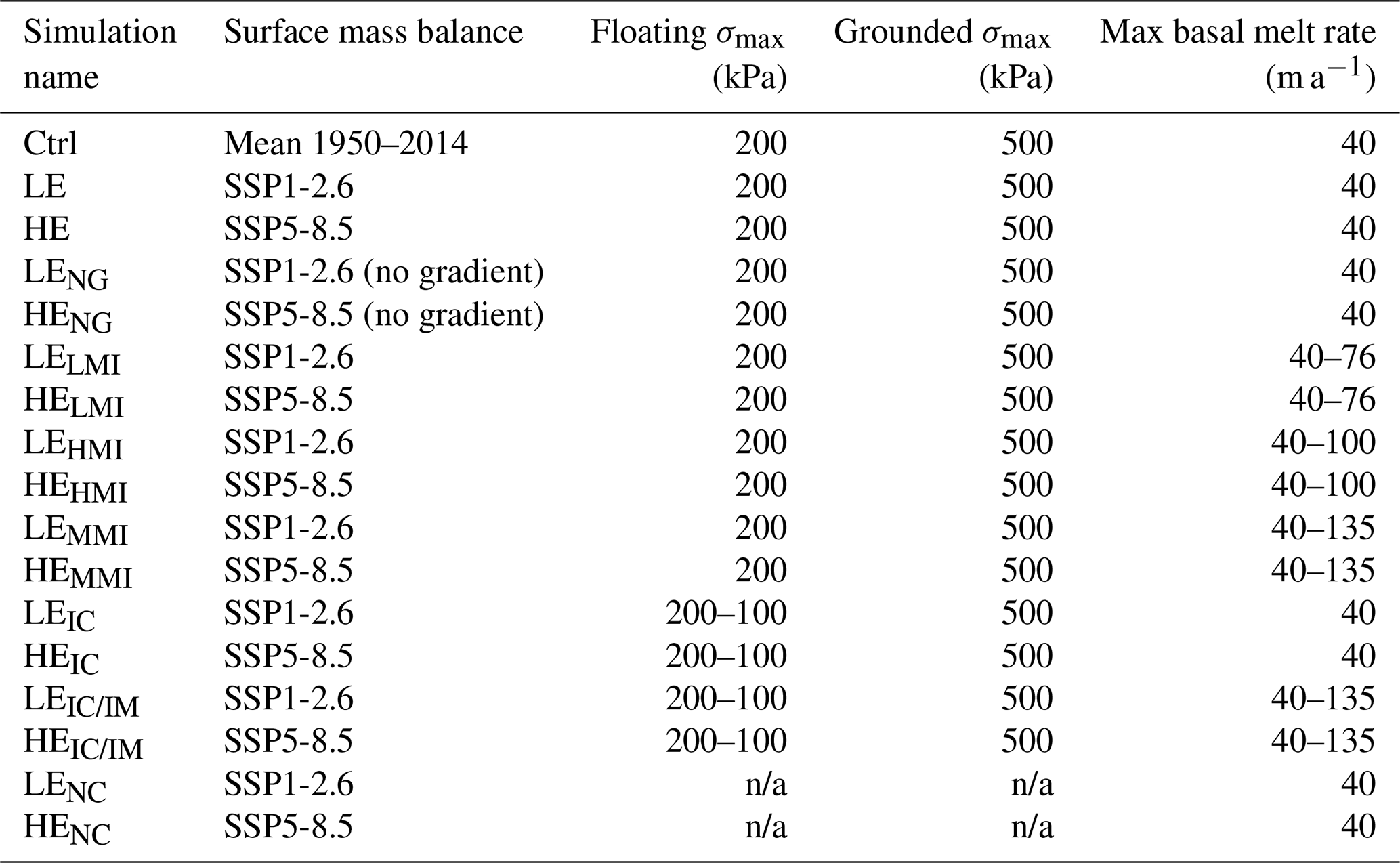
n/a: not applicable.

Two of the simulations, low emissions (LE) and high emissions (HE), impose different SMB scenarios (SSP1-2.6 and SSP5-8.5 respectively) whilst keeping the calving and ocean-driven melt parameters at present-day values. The no-gradient (NG) simulations, LE_NG and HE_NG, are the same as the former, except that in these simulations – and only in these simulations – the SMB–elevation feedback is not included. Three different ocean-driven melt rate increase scenarios are then tested: a low melt increase (LMI), a high melt increase (HMI), and a maximum melt increase (MMI). For the LMI scenario, we assume a linear increase in ocean temperatures relative to the present day of 1 °C by 2100, 2 °C by 2200, and 3 °C by 2300. Each of these 1 °C increases corresponds to a 12 m yr⁻¹ increase in submarine melt rates, which should be considered a low-end estimate for Ryder Glacier (Wiskandt et al., 2023). For the HMI scenario, we assume the same increase in ocean temperatures but impose an additional 20 m yr⁻¹ of submarine melt per degree of ocean warming – a high-end estimate for Ryder Glacier (Wiskandt et al., 2023). For the MMI scenario, we draw on insights from Wekerle et al. (2024) and impose a nonlinear increase in melt rates for each degree of ocean warming to represent processes such as increases in subglacial discharge with time. Here, we impose an increase of 20 m yr⁻¹ for the first degree of warming by 2100, followed by an increase of 25 m yr⁻¹ for the second degree of warming towards 2200, and finally an increase of 30 m yr⁻¹ for the third degree of warming by 2300. Furthermore, we look into the possibility of increased calving (IC) in the future by reducing the stress threshold for floating ice linearly with time, both with a constant submarine melt rate (experiments LE_IC and HE_IC) and in combination with the maximum prescribed increase in submarine melt rates (experiments LE_IC/IM and HE_IC/IM). To assess the impact of neglecting calving in model simulations, simulations with no calving are also run (experiments LE_NC and HE_NC). All of these scenarios are run with SMB forcing from both SSP1-2.6 and SSP5-8.5.

3 Results

3.1 Sea level rise contribution

In the control (Ctrl) simulation, where SMB was set to equal the mean of the 1950–2014 SMB fields, overall mass loss was the lowest out of all simulations. The sea level rise contribution in 2300 from this simulation was 0.3 mm, which includes both committed sea level rise and model drift.

The cumulative sea level rise contribution from all low- and high-emission scenarios is shown in Fig. 3. Here, it is seen that the sea level rise contribution from the low-emissions scenarios varies between 0.8 and 2.0 mm by 2300. Subtracting the sea level rise contribution from the Ctrl simulation shows that, under SSP1-2.6, between 0.5 and 1.7 mm of sea level rise from Ryder Glacier is due to future changes in external forcing. Most of the low-emissions scenarios lead to somewhere between 0.8 and 0.9 mm of sea level rise, but there are a few exceptions. The first of these is the LE_NC simulations, where no calving was allowed and a total sea level rise (SLR) contribution of only 0.68 mm was seen. On the other end of the spectrum, the simulations LE_MMI and LE_IC/IM show a higher contribution of nearly 2.0 mm. These high-SLR-contribution simulations follow a similar trajectory to all other LE simulations up until the late 2200s, after which their mass loss accelerates. The shared feature between these two simulations is that they both include the maximum increase in submarine melt, where a nonlinear relationship between ocean temperatures and basal melt rates is assumed. In both of these simulations, the high level of basal melt causes the glacier to retreat into bedrock depression – retreat through which is associated with the rapid increase in mass loss and terminus retreat seen in Fig. 3.

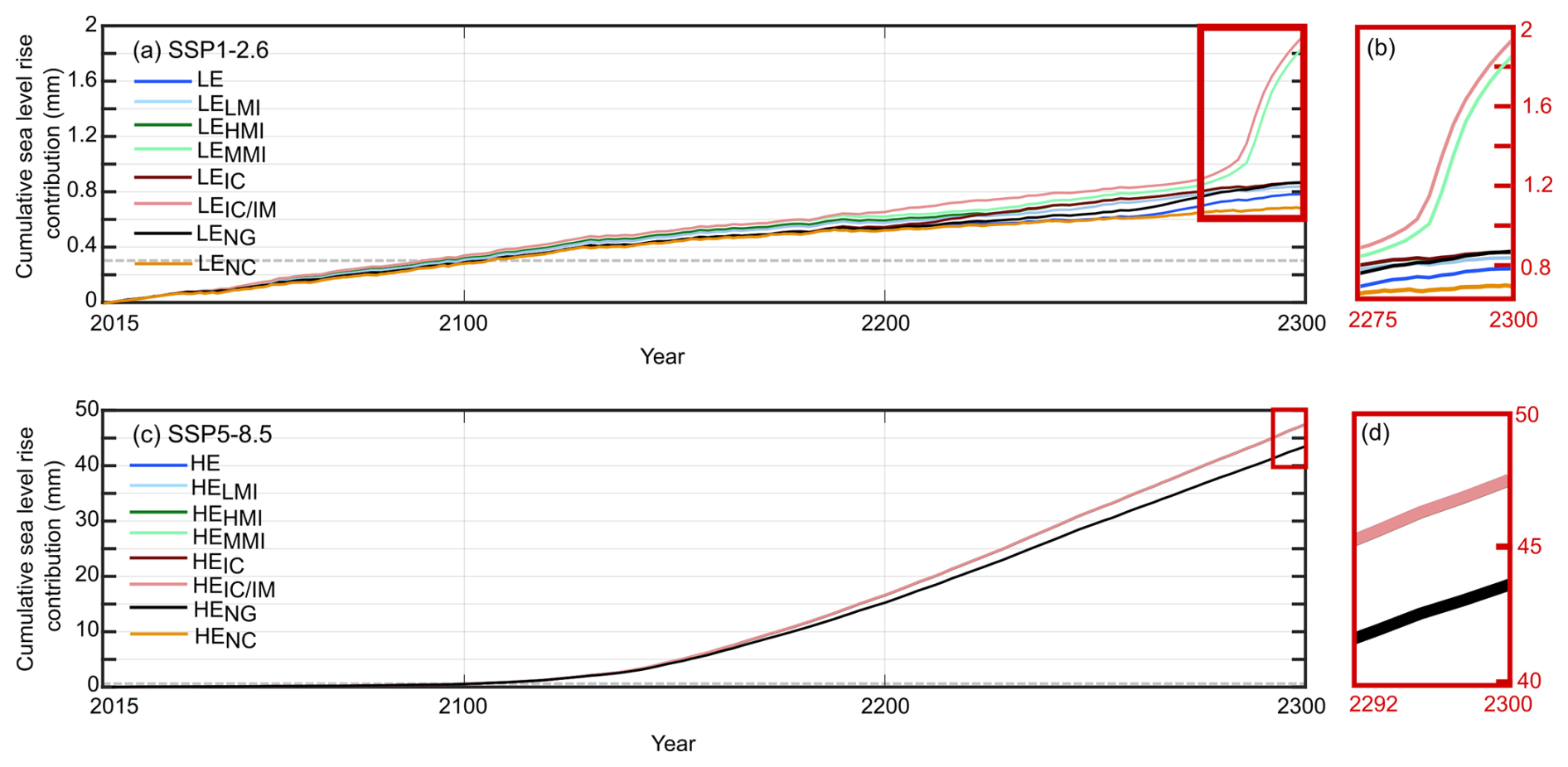
Figure 3 Cumulative sea level rise contribution in millimetres for all low-emissions simulations for 2015–2300 is shown in (a), with a close-up of 2275–2300 shown in (b). Cumulative sea level rise for all high-emissions simulations for 2015–2300 is shown in (c), with a close-up for 2292–2300 shown in (d). In the high-emissions simulations, all the simulations except for HE_NG (no gradients) show the same sea level rise contribution curve, meaning that they overlap, and it is not possible to discern the different lines on the plot – even when zoomed in. Note the different y axes used for the low- and high-emissions scenarios. In panels (a) and (c), a dashed grey line denotes the sea level rise contribution of 0.3 mm from the Ctrl simulation.

In the high-emissions scenarios, all the simulations, with the exception of HE_NG, show an almost identical trajectory in terms of sea level rise contribution. By 2300, all of these simulations lead to ca. 47 mm of sea level rise, of which ca. 46.7 mm can be attributed to changes in external forcing by subtracting the results from the Ctrl simulation. In contrast, the HE_NG simulation leads to 44 mm of sea level rise (43.7 mm when subtracting the Ctrl simulation). All of these sea level contributions are over 40 mm greater than the sea level contribution from any SSP1-2.6-forced simulations. Ryder Glacier currently holds enough ice to contribute 129 mm to sea level rise, meaning that these modelled sea level rise contributions correspond to almost one-third of the total sea level rise potential.

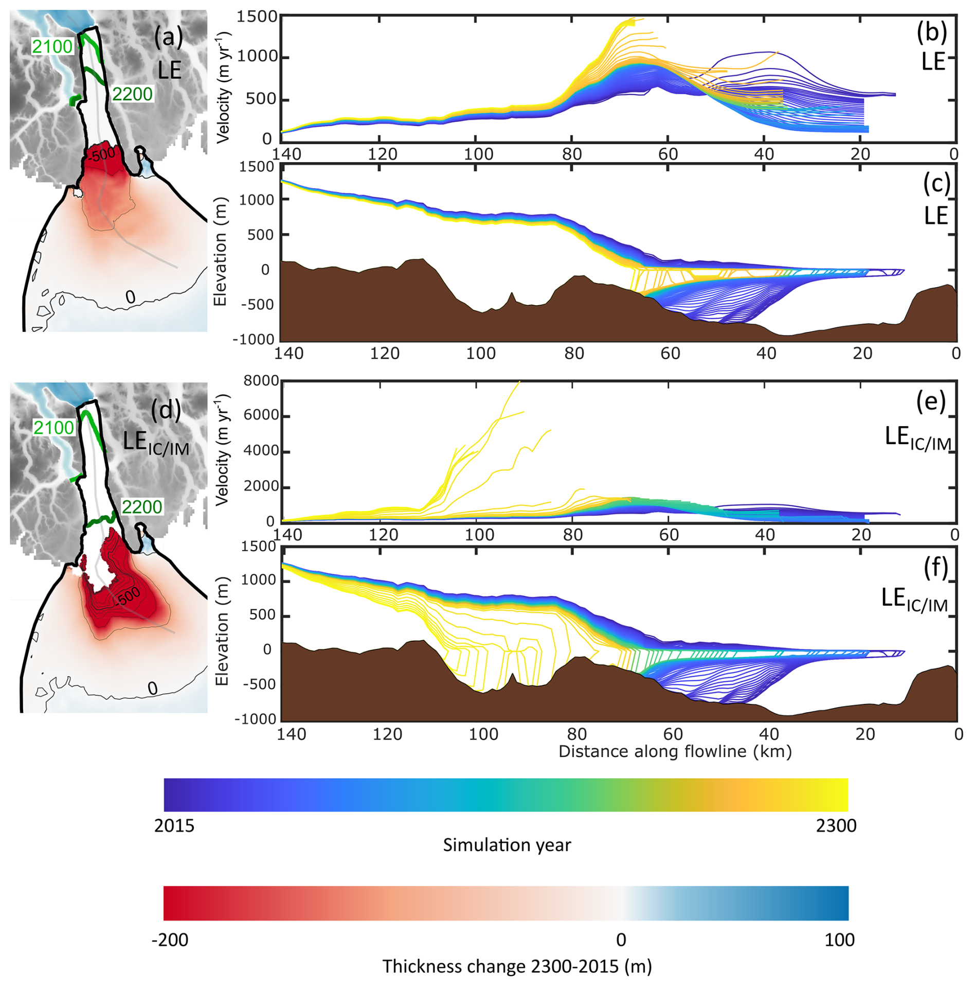
Figure 4 Changes in front position, velocity, and ice thickness from LE (a–c) and LE_IC/IM (d–f). The thickness change between 2015 and 2300 is shown in panels (a) and (d), where the front positions in 2100 and 2200 are shown. The front position in 2300 corresponds to the limit of the thickness change map. Contours of thickness change are also shown, with thin lines denoting 100 m of change and the bold lines denoting 500 m of change. Panels (b) and (e) show velocity along a flowline with time (note the different y-axis scales), and panels (c) and (f) show glacier geometry along a flowline with time. The flowline follows the retreating glacier front and is shown as a pale grey line in panels (a) and (d). Bedrock topography, bathymetry, and ice mask data are from BedMachine v5 (Morlighem et al., 2017).

3.2 Terminus retreat and glacier dynamic response

The terminus retreat, velocity changes, and thinning magnitude are shown in Fig. 4 for the LE and LE_IC/IM simulations and in Fig. 5 for the HE and HE_IC/IM simulations. These simulations were chosen as they constitute the simulation where only SMB was changed compared to the relaxation, as well as the simulation in each scenario with the greatest mass loss. Common between all LE and HE simulations is a trend of retreat and thinning during the 2015–2300 period. This is in contrast to the Ctrl simulation, where limited thinning and retreat leads to the ice tongue persisting all the way to 2300. In the Ctrl simulation, the terminus also remains mostly stable but exhibits a retreat of 6 km at its eastern margin. Grounding line retreat of ca. 7.7 km is seen at the centreline.

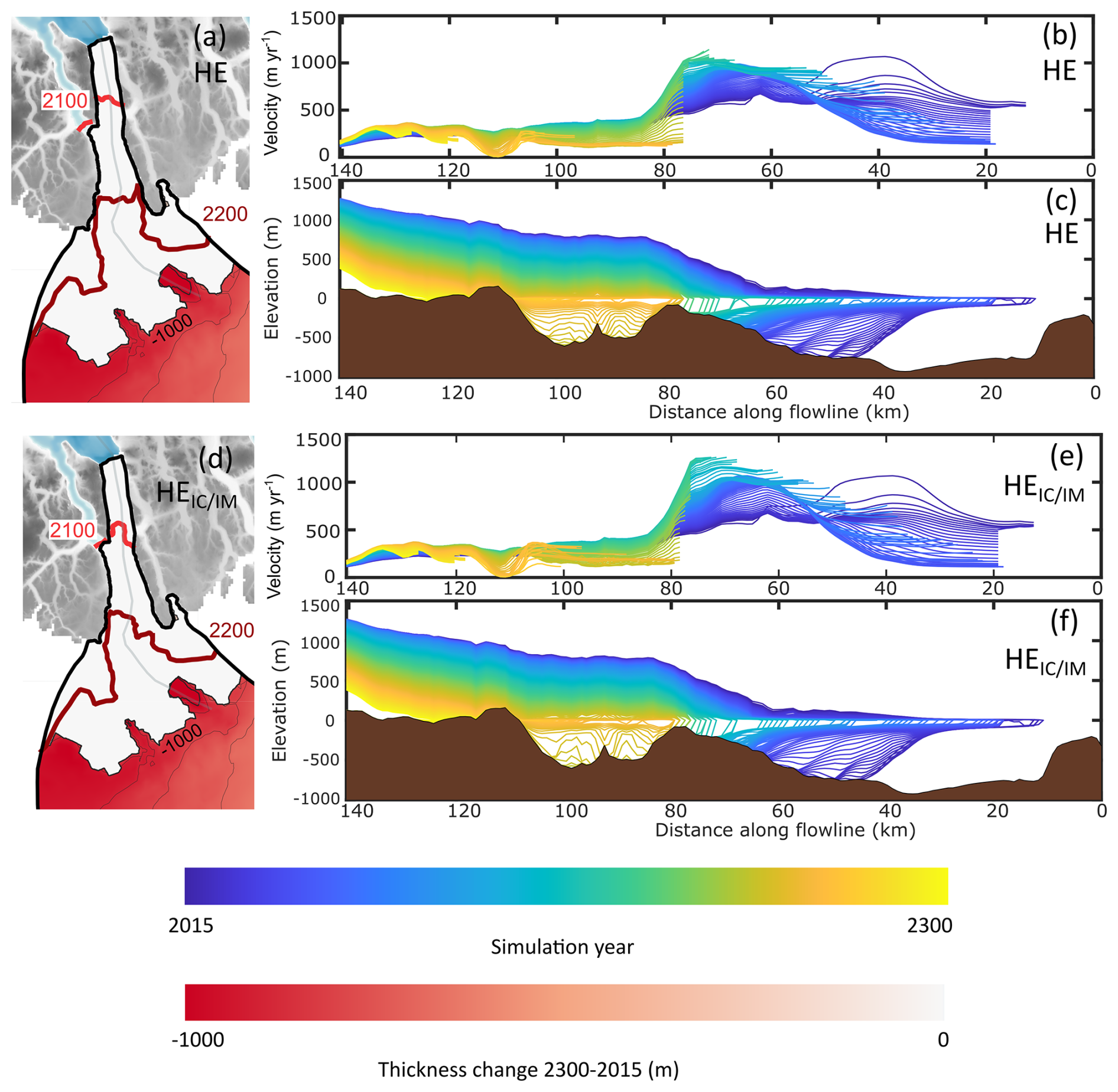
Figure 5 Changes in front position, velocity, and ice thickness from HE (a–c) and HE_IC/IM (d–f). The thickness change between 2015 and 2300 is shown in panels (a) and (d), where the front positions in 2100 and 2200 are shown. The front position in 2300 corresponds to the limit of the thickness change map. Contours of thickness change are also shown, with thin lines denoting 100 m of change and the bold lines denoting 500 m of change. Panels (b) and (e) show velocity along a flowline with time, and panels (c) and (f) show glacier geometry along a flowline with time. The flowline follows the retreating glacier front and is shown as a pale grey line in panels (a) and (d). Note that the thickness change scale is different than that used in Fig. 4. Bedrock topography, bathymetry, and ice mask data are from BedMachine v5 (Morlighem et al., 2017).

In all the low-emissions scenarios with the exception of LE_NC, the ice tongue is always lost by 2300, although it is already lost by 2200 during the two simulations in which the maximum increase in melt rates is applied (LE_MMI and LE_IC/IM). The magnitude of retreat varies considerably between low-emissions scenarios with the LE_IC/IM and LE_MMI simulations (where the maximum melt rate increase is applied), exhibiting nearly 100 km of retreat by 2300, whereas the other scenarios, such as the LE simulation (with no melt rate increase), only exhibit around 60 km of retreat. This shows that thinning of the ice tongue from ocean-driven melt is a key driver of ice-tongue loss in, playing a more important role than increased calving in response to, for example, a reduction in sea ice. In the simulations showing the most retreat (LE_IC/IM and LE_MMI), the retreat occurs gradually until the retrograde slope located around 80 km along the flowline is reached, after which rapid retreat occurs before re-stabilisation on the prograde slope at 110 km (Fig. 4). By this point, Ryder Glacier's terminus is partly land terminating and partly marine terminating. Although all low-emissions simulations show increasing frontal velocities with time, this rapid retreat along a retrograde slope is associated with a short-term increase in frontal velocities from circa 1000 to 8000 m yr⁻¹ (Fig. 4). All the low-emissions simulations show a similar pattern of strong thinning of up to 200 m near the glacier terminus, with this extending ca. 50 km inland. Further upstream, areas with both slight thinning and thickening are seen (Fig. 4). The outlier to the trend of ice-tongue loss is the LE_NC simulation, where the ice tongue remains all the way to 2300. In this simulation, grounding line retreat of ca. 21 km is seen, which is of a similar magnitude to that of other LE simulations without increased melt rates (see Fig. 4a). However, terminus retreat was limited, ranging from only 9 km at the centreline to 16 km at the eastern margin.

In the high-emissions scenarios, the ice tongue is lost in all simulations by 2200, with overall higher levels of retreat and thinning compared to the low-emissions scenarios. Here, ice-tongue disintegration is driven by thinning as a result of the strongly negative SMB over the ice-tongue/lower ablation area. Little variation is seen between the different high-emissions scenarios – including the HE_NC simulation. In all simulations, including the HE and HE_IC/IM simulations shown in Fig. 5, the glacier front retreats by over 110 km. Frontal velocities initially increase as the ice tongue is lost, before decreasing after 2200 (Fig. 5be). The entire glacier domain experiences significant thinning by 2300, with frontal areas showing thinning of around 1 km (Fig. 5a, d).

In all simulations, both low and high emissions, the grounding line/grounded terminus position tends to stabilise (or retreat more slowly) on bedrock highs or prograde slopes (Figs. 4c, f and 5c, f). In any simulation where the grounding line retreats upstream of the bedrock sill at around 80 km along the flowline, retreat occurs rapidly (ca. 2000 m yr⁻¹) before the glacier regains some stability on the bedrock high at around 110 km along the flowline.

The retreat of both the grounding line and the glacier terminus in LE, LE_IC/IM, HE, and HE_IC/IM is shown in Fig. 6 alongside the mean frontal velocity from the same simulations. Here, it is clear that under a low-emissions future, the ice tongue may be lost anytime between 2200 and 2300, depending on ocean forcings – a large temporal range of up to a century. In addition, the mean frontal velocity tends to increase simultaneously with periods of ice-tongue collapse or rapid terminus retreat, as evidenced by the spike in frontal velocities of up to 2000 m yr⁻¹ in the latter half of the 2200s in Fig. 6a.

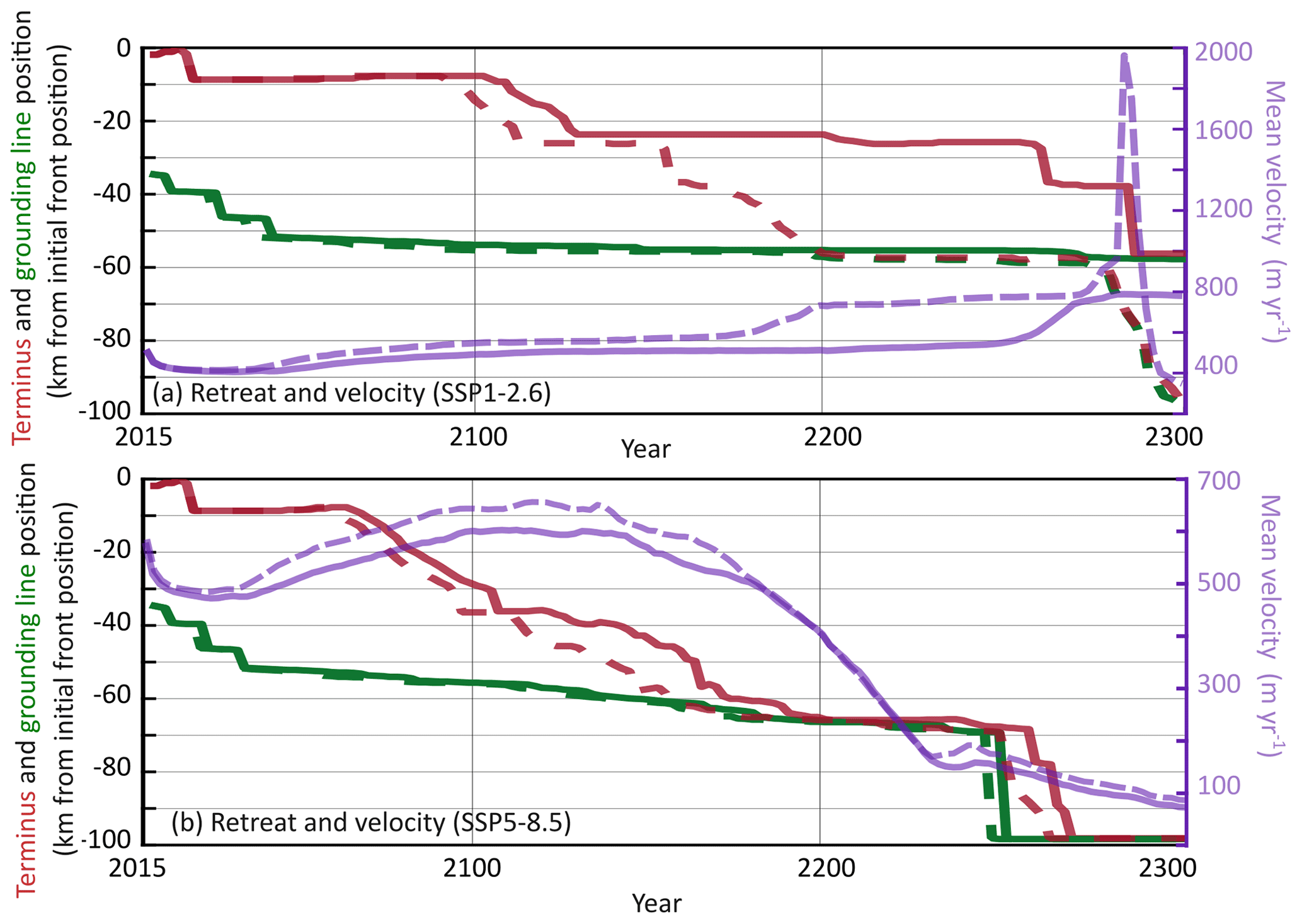
Figure 6 Retreat of the glacier front (magenta) and grounding line (green) for low- and high-emissions scenarios is shown in panels (a) and (b) respectively. The solid lines denote the simulation exhibiting the least mass loss (LE and HE_NG), and the dashed lines show the simulation exhibiting the most mass loss (LE_IC/IM and HE_IC/IM). Where the magenta and green lines meet, the glacier no longer has a floating ice tongue. The purple lines denote the mean velocity of the near-terminus grounded areas and uses the y axis on the right-hand side of each plot. The near-terminus grounded areas are defined as all grounded parts of the glacier within 500 m of the grounding line at each time step. Note the different y-axis scales for the different emissions scenarios.

This trend is also seen in the high-emissions simulations, where velocities are elevated from ca. 2050 until ca. 2200 during a period of ice-tongue retreat. The data from HE and HE_IC/IM show very similar trajectories but with a offset of ca. 10–20 years.

3.3 Mass loss partitioning

The partitioning of mass loss between SMB and discharge (calculated as total mass loss – SMB) for the mean of the low- and high-emissions scenarios is shown in Fig. 7. In a low-emissions future, discharge is consistently the driver of overall mass loss – with SMB remaining slightly positive all the way to 2300 as a result of the large accumulation zone. A large increase in discharge around 2280 in LE_MMI (Fig. 7f) corresponds to the retreat of the glacier into a deep basal trough, with these increases in discharge starting to stabilise once a bedrock high is reached.

In all high-emissions scenarios, discharge plays a dominant role in driving mass loss trends up until 2100, after which SMB becomes more significant and mass losses accelerate overall (Fig. 7). Despite this, discharge in the high-emissions simulations remains higher than discharge in the low-emissions simulations (Fig. 7). The strongly negative SMB in the high-emissions simulations leads to thinning over the entire model domain and a situation in which overall mass loss is mostly unaffected by the decision to exclude calving in HE_NC (Fig. 5).

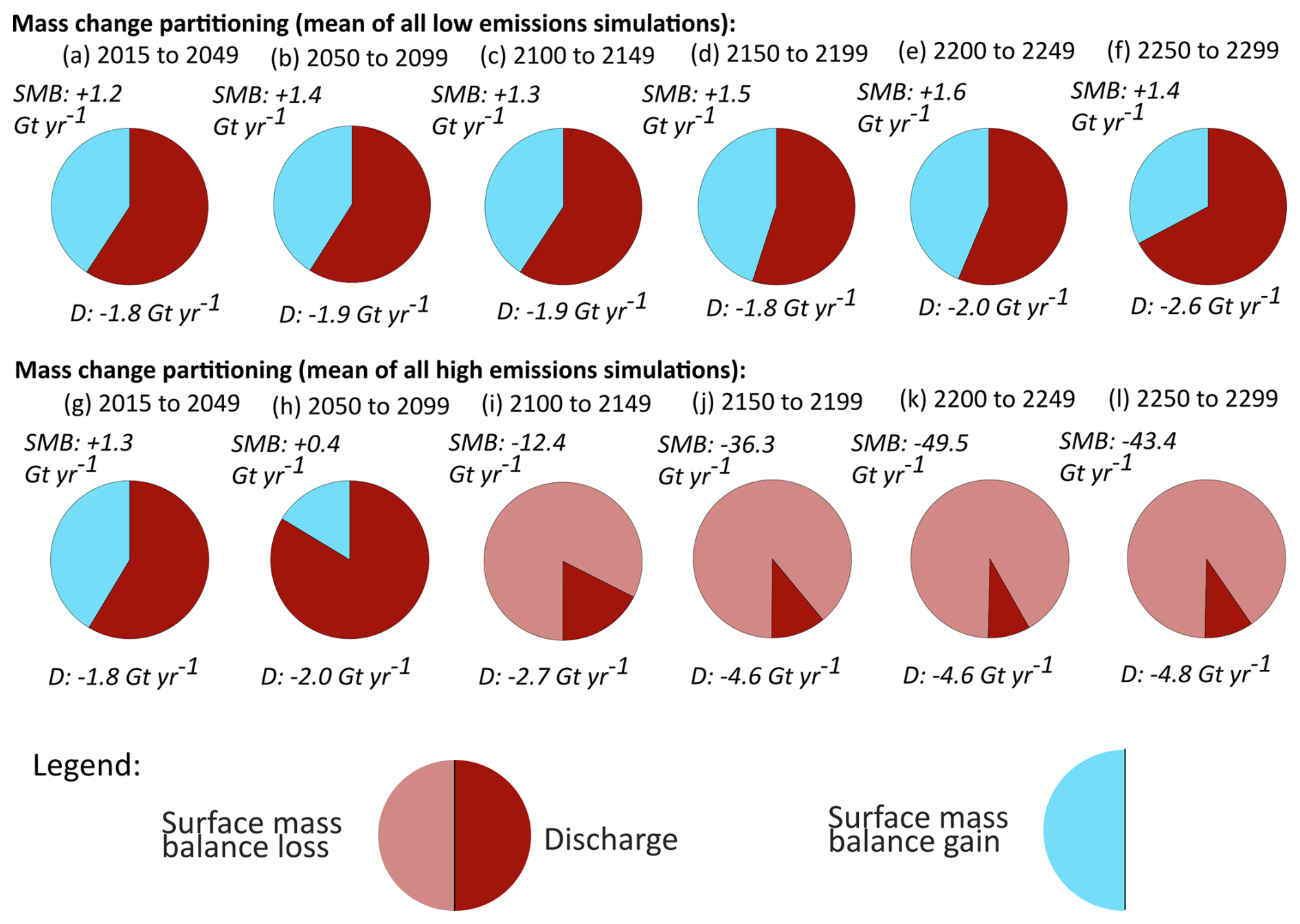
Figure 7 The partitioning of mass change between SMB and discharge for the mean of all low-emissions simulations (a–f) and all high-emissions simulations (g–l) for the periods of 2015 to 2049, 2050 to 2099, 2100 to 2149, 2150 to 2199, 2200 to 2249, and 2250 to 2300.

4 Discussion

4.1 Influence of emissions scenario

Stark differences can be seen between the simulations using a low-emissions scenario and those using a high-emissions scenario by 2300 – although all simulations show mass loss dominated by discharge up until 2100. Most importantly, sea level rise contributions differ by an order of magnitude. Under a low-emissions scenario, at least 0.5 mm of sea level rise is attributable to changing external forcings compared to at least 43.7 mm under a high-emissions scenario. As the suite of low- and high-emissions simulations was run using the same initialised state, and with the same set of oceanic forcings, the differences between the corresponding low- and high-emissions simulations can be attributed to the SMB alone, even if the magnitudes of ocean warming and subglacial discharge are likely to vary depending on the future emissions scenario. The fact that we see the greatest differences between the simulations with different SMB scenarios, rather than between the simulations forced with different submarine melt rates, suggests that SMB exerts a dominant control on Ryder Glacier's future trajectory. Several Greenland-wide modelling studies have also found that SMB is an important driver of future mass loss, but there is significant spread between the magnitude of mass loss between different studies. A study by Aschwanden et al. (2019), which modelled Greenland up until the year 3000, found that the sea level contribution from Greenland in 2300 was likely to be ca. 25 cm under RCP 2.6 (comparable to SSP1-2.6) and ca. 174 cm under RCP 8.5 (comparable to SSP5-8.5). These sea level rise contributions correspond to 3.4 % and 24 % of Greenland's sea level rise potential respectively. In the simulations presented here, the sea level rise contribution from Ryder Glacier is 0.8–0.2 cm under SSP1-2.6 and 4.4–4.7 cm under SSP5-8.5. The total potential sea level rise contribution from Ryder Glacier is 12.9 cm, meaning that these values correspond to 0.6 %–1.5 % (SSP1-2.6) or 34 %–37 % (SSP5-8.5) of Ryder Glacier's sea level rise potential. Therefore, our simulations show a smaller percentage-wise sea level rise contribution under SSP1-2.6 compared to the Greenland-wide study but a larger percentage-wise sea level rise contribution under SSP5-8.5. However, our sea level rise contribution under SSP5-8.5 is smaller than that found by another Greenland-wide modelling study by Beckmann and Winkelmann (2023), which focuses on extreme events and thus likely constitutes an end-member scenario. Compared to the results of ISMIP6 (Goelzer et al., 2020), which only includes simulations up to 2100, our SSP5-8.5 results for Ryder fit within the given range of sea level rise contribution for northern Greenland, where between ca. 5 %–15 % of northern Greenland's potential sea level rise contribution is simulated to occur. Additionally, the results of ISMIP6 show that northern Greenland has a relatively low sensitivity to ocean forcing under a high-emissions scenario – something we also find in this study for Ryder Glacier. Although our results therefore fit within the range of previous studies, the differences that do occur between our results and the aforementioned papers are partly due to the fact that the development of Ryder Glacier as an individual outlet glacier is not expected to follow the same trajectory as that of the Greenland Ice Sheet as a whole. However, due to the lack of previous studies dedicated to Ryder Glacier, it is not possible to make more targeted comparisons. These differences between the trajectories modelled for Ryder Glacier and the entire ice sheet may be because the higher mesh resolution employed here on the smaller domain allows for site-specific characteristics, such as bed topography, to be well resolved, allowing for behaviours related to marine ice sheet instability to be fully captured by the model. As such, running high-resolution studies that focus on individual glaciers or regions is vital for validating the results from broader-scale studies that must, for computational reasons, employ a coarser grid resolution.

The simulations forced with an SSP5-8.5 future showed less sensitivity to variations in ocean forcing compared to the simulations forced with an SSP1-2.6 future. In Fig. 3, all the high-emissions simulations follow the same indistinguishable trajectory, with the exception of HE_NG, where no SMB–elevation feedback was incorporated. This relationship between glacier behaviour and ocean melt under different emissions scenarios is something not considered in other studies, where the Greenland-wide focus meant ocean-induced melt rates were fixed in time (Beckmann and Winkelmann, 2023) rather than increasing, in line with results from site-specific modelling and observational studies (Wilson et al., 2017; Wiskandt et al., 2023). The results of HE_NG are very similar to those of the other high-emissions scenarios until around ca. 2150, after which they start to diverge, corresponding to the onset of extensive thinning at Ryder Glacier. The SMB–elevation feedback has previously been identified as a key driver of runaway melt and retreat of the Greenland Ice Sheet (Bochow et al., 2023), something that we also find here. However, it is also possible that this implementation leads to an overestimation of retreat as the lapse rates used are not fully valid at ice sheet margins (Delhasse et al., 2024). Specifically, our results show that the exclusion of this feedback has a greater impact on the modelled sea level rise contribution results than the chosen basal melt rate scenario, at least for the high-emissions simulations. The SMB–elevation feedback is likely particularly important for glaciers in the northern sector of the Greenland Ice Sheet as the gently sloping margins in the area result in some of the fastest rates of upward migration of the ablation zone and runoff line (the upper extent of where runoff exceeds 100 mm w.e. yr⁻¹) across all of Greenland (Noël et al., 2022a). In combination with this, the interior of the northern sector has a generally lower elevation than the northeastern and northwestern sectors, a characteristic which lends itself to accelerated mass loss (Noël et al., 2022a). Incorporating this SMB–elevation feedback into models has led to increases in the expected mass loss from the northern sector (Muntjewerf et al., 2020), something also seen in this study when comparing the HE (SMB–elevation feedback included) and HE_NG (no SMB–elevation feedback) simulations. In the low-emissions simulations, the simulation without the SMB–elevation feedback (LE_NG) fits well within the range of the other low-emissions simulations – likely reflecting the minor effect of the SMB–elevation feedback in a situation where thinning of the ice sheet surface is much more limited.

4.2 Drivers of mass loss

In the low-emissions simulation, there is a clear increase in frontal velocities associated with front retreat and ice-tongue loss. For example, in Fig. 4b, the frontal velocities increase from around 750 m yr⁻¹ to around 1500 m yr⁻¹ within the last 50 years or so of the simulation, corresponding to the complete loss of the ice tongue, as shown in Fig. 4c. However, this effect is seen not only when the ice tongue is lost, but also during periods of rapid retreat of the grounded glacier front. This is exemplified in Fig. 4e, f, where the rapid retreat of Ryder Glacier across a bathymetric trough in the late 2200s is associated with frontal velocities that reach over 8000 m yr⁻¹. This is an over 4-fold increase in frontal velocity (see Fig. 6) and is associated with a thinning of the glacier frontal region of the order of several hundreds of metres over a period of ca. 15 years. This period of acceleration and thinning begins where the then-grounded glacier front retreats onto a retrograde slope and into a bathymetric depression, thus highlighting the strong coupling between bedrock topography and mass loss (Schoof, 2007; Schoof et al., 2017). This period of rapid retreat, acceleration, and thinning is only seen in the LE_MMI and LE_IC/IM simulations, where the increased ocean-driven melting is sufficient to retreat the glacier onto the retrograde slope. By 2300, the glacier has somewhat stabilised on the prograde slope at the landward side of the bathymetric depression, with subdued retreat rates and a decrease in frontal velocities down to ca. 4000 m yr⁻¹. However, by this point, the discharge from these simulations has caused a spike in mass loss and sea level rise contribution, as can be seen in Fig. 3. Although Ryder Glacier is still grounded below sea level, the basal topography at this point is shallow and, in parts, even above sea level. Further retreat would lead to a greater proportion of Ryder Glacier becoming land terminating, meaning that it is unlikely to undergo any further periods of rapid ocean-driven mass loss.

Although all the high-emissions simulations also show Ryder Glacier retreating through this bathymetric trough, there is no clear dynamic response in these simulations. Instead, both simulations shown in Fig. 6 show acceleration between 2080 and 2150 as the ice tongue shrinks, with a deceleration then being seen after ice-tongue loss – something that coincides with an acceleration of SMB-driven thinning. When the glacier then retreats through the bathymetric trough, the glacier has already thinned so much due to a negative SMB (i.e. surface melt) that mass loss is dominated by downwasting near the front rather than ocean-driven retreat. This is combined with the fact that Ryder Glacier has retreated to shallower ground by this point and is, in some parts, land terminating. Only the central part of the terminus remains marine terminating, with the entire glacier projected to become grounded above sea level with an additional ca. 9 km of retreat. As a result, ocean-driven forcing is not as important for the overall mass balance in 2300 as it is in the present day. However, there is still evidence of bathymetric control up until ca. 2100; the retreat of the grounding line from its present-day position up the prograde slope is interrupted by short stillstands on small bathymetric ridges. This acceleration towards 2200 followed by a deceleration is consistent with patterns found by Beckmann and Winkelmann (2023) for the northern sector from a Greenland-wide modelling study. In their study, extensive thinning and the associated decrease in driving stress were suggested as the cause of slower velocities after 2200 – something that we also propose as the reason for the reduced velocities after ca. 2200 here.

Considered together, both the low- and the high-emission simulations provide evidence of a dynamic response to ice-tongue loss at Ryder Glacier. This suggests that the ice tongue currently exerts a buttressing force on the grounded areas of the glacier and that mass loss and sea level rise contribution from Ryder are likely to increase in conjunction with a potential future ice-tongue disintegration. This result, suggesting a dynamic response after ice-tongue collapse at Ryder Glacier, may therefore provide insight into how other Greenlandic glaciers with ice tongues may behave in the future, which is especially important given that previous studies have found that model uncertainties are higher for glaciers with ice tongues in Greenland-wide set-ups (Choi et al., 2021).

We find clearly contrasting drivers of mass loss across the suite of low-emissions simulations compared to the suite of high-emissions simulations. As shown in Fig. 7, Ryder Glacier experiences an overall positive SMB during the entirety of the modelled period, although the frontal region of the glacier experiences a net negative SMB. This may be in contrast to trends over the entire northern sector, where SMB has been net negative since around the year 2000, but when considering Ryder Glacier by itself, there has been a net positive SMB of 2.1 Gt yr⁻¹ in the 2000–2017 period (Mouginot et al., 2019). In the simulations presented here, net SMB is lower than the 2000–2017 mean but does not change significantly throughout the study period, with discharge losses driving overall mass loss. The magnitude of these discharge losses consistently outweighs the positive surface mass balance, leading to an overall mass loss of around 0.65 Gt yr⁻¹ averaged across the entire study period. This is lower than the mean mass balance of −0.96 Gt yr⁻¹ for the 2000–2017 period but significantly more negative than the mean mass balance of +0.33 Gt yr⁻¹ observed during the 1972–1990 period. The lack of an increased mass loss under a low-emissions scenario likely reflects the fact that the accumulation zone of Ryder Glacier is large and retains a net positive SMB during the entire study period. As the ice tongue is lost and Ryder Glacier's front retreats by several tens of kilometres, large swathes of the current ablation zone are removed. At the same time, the shallowing basal topography inland of Ryder Glacier's present-day grounding line – albeit it with some basal troughs – means that the impact of ocean forcing and discharge-driven mass loss is constrained. Together, these features (which are specific to the bathymetry of Ryder Glacier and to the low-emissions scenario) act to modulate future mass loss. This geometric control on Ryder Glacier's future behaviour highlights the need for high-resolution studies that can resolve topographic features under individual outlet glaciers, providing results which can inform and validate Greenland-wide studies.

The pattern of SMB and discharge trends is significantly different for the high-emissions simulations, where the SMB is positive until 2099, after which it decreases significantly to become the dominant driver of mass loss from 2100 onwards. Discharge is, like in the low-emissions simulations, a key driver of mass loss until 2099, after which it is dwarfed by SMB-driven losses. By 2300, SMB losses are an order of magnitude higher than discharge, and little variation is seen between simulations. Under SSP5-8.5, temperatures in the Arctic are projected to increase drastically by 2100, becoming ca. 10 °C warmer than during the 1995–2014 period (Lee et al., 2021). This is significantly higher than the expected global temperature anomaly of 4 °C as a result of ongoing Arctic amplification (Rantanen et al., 2022). Moreover, this is higher than projected temperature changes under SSP1-2.6, where the Arctic is expected to experience temperatures 2.4 °C warmer than mean 1995–2014 values, with the global mean temperature anomaly expected to be only 0.7 °C (Lee et al., 2021). The gap between these scenarios continues to grow past 2100 and, in the case of SSP5-8.5, the lowering of the ice sheet surface further exacerbates the local SMB anomaly. As such, Ryder Glacier is likely to exhibit extensive thinning across its entire drainage basin under an SSP5-8.5 future, with discharge losses playing a relatively insignificant role despite being considerably higher than in the present.

These results suggest that the future emissions path, and associated atmospheric warming, exerts a dominant control on overall mass loss, with the largest variations seen between the low- and high-emissions simulations rather than within them. However, discharge will play a key role in driving mass loss at Ryder until 2100 regardless of the emissions scenario. This result corroborates well with that of Choi et al. (2021), who found that ice dynamics would likely be a key driver of mass loss from Greenland during the next century but with SMB playing an increasingly important role as time goes on. This study adds to these conclusions by continuing simulations past 2100, showing that SMB-driven loss rapidly surpasses discharge loss post-2100 in a high-emissions future. Additionally, bathymetry plays a significant role in determining shorter-term variability, with periods of acceleration and elevated mass loss being associated with retrograde slopes and deeper basins.

4.3 Comparisons with other glacier–fjord systems

The finding that Ryder Glacier's ice-tongue collapse leads to a dynamic response at first appears to be at odds with observations from the neighbouring Petermann Glacier, where large calving events in 2010 and 2012 have been associated with a limited dynamic response (Münchow et al., 2014; Nick et al., 2012). However, modelling work at Petermann Glacier shows that potential future calving events closer to the grounding line are likely to cause large increases in velocity and discharge (Hill et al., 2018a; Åkesson et al., 2022). At Ryder Glacier, the modelling experiments presented here all exhibit total ice-tongue loss, with these events therefore being, by definition, in close proximity to the grounding line. As such, the associated accelerations and increase in discharge are similar to those projected to occur under similar circumstances at Petermann Glacier. This is in contrast to the limited dynamic response observed after the 2002–2003 collapse of C.H. Ostenfeld Glacier's ice tongue (Hill et al., 2018a). This is likely linked to ice-tongue/fjord geometry, where the buttressing afforded by an ice tongue is likely lower in glacier–fjord systems where there is little contact between the lateral margins of the ice tongue and the fjord walls – as was seen at C.H. Ostenfeld Glacier prior to collapse (Hill et al., 2017). These findings are relevant to Greenland's largest ice tongue, 79N (Nioghalvfjerdsfjorden) Glacier, which, like Ryder Glacier, has experienced limited volume change in recent decades, despite evidence of Warm Atlantic Intermediate Water near its grounding line (Millan et al., 2023; Bentley et al., 2023). 79N Glacier's ice tongue is attached to the adjacent fjord walls, with the ice tongue narrowing ca. 20 km inland of its present-day terminus position. Our model findings for Ryder Glacier suggest that the fjord geometry at 79N Glacier may help keep the terminus position relatively stable, despite being subject to the highest basal melt rates out of all the Greenlandic glaciers with ice tongues (Wekerle et al., 2024). However, the strong traction between the ice tongue and fjord walls at 79N Glacier also suggests that the ice tongue plays an important role in terms of buttressing, with evidence of acceleration in response to thinning having already been documented (Khan et al., 2022).

These findings also have implications for glaciers without ice tongues and highlight the important role of fjord geometry in moderating glacier response to external forcings (Catania et al., 2018). The impact of fjord geometry on glacier stability has previously been studied, although often with the use of simplified synthetic geometries (e.g. Åkesson et al., 2018; Frank et al., 2022). The differing behaviour of the Ryder, Petermann, and C.H. Ostenfeld glaciers showcased here highlights how these topographical controls can lead to highly heterogenous behaviour in real-world neighbouring systems. Ryder Glacier's recent lack of terminus retreat may, in part, be a consequence of its narrow fjord (when compared to e.g. Petermann Fjord) (Frank et al., 2022), which may provide an explanation for how Ryder Glacier has exhibited little terminus retreat despite reports of basal melt rates exceeding those at Petermann Glacier (Millan et al., 2023). Additionally, the rapid retreat of Ryder Glacier in the low-emissions scenarios once a retrograde bed slope is reached illustrates that seemingly stable glaciers can suddenly exhibit rapid retreat, having been in a state of disequilibrium with the ambient climate (Robel et al., 2022). However, it is also important to note that the rapid retreat ceases when a prograde slope is reached – showing how bathymetry can also act to stabilise glaciers and prevent runaway retreat. Understanding these processes is vital for accurately forecasting the timing of glacier retreat and associated sea level rise (Robel et al., 2022). This suggests that once a threshold is reached – which may occur asynchronously with climate forcing due to geometry-imposed stability or as a result of sustained change over several years – drastic increases in velocity and discharge may occur. These losses are inherently difficult to predict, not least considering the uncertain shape of the seafloor and under-ice topography. In addition, the shallow bathymetric sill which sits in front of Ryder Glacier’s grounding line has been documented to block intrusions of warm Atlantic water (Jakobsson et al., 2020). Importantly, this reduces the basal melt and its sensitivity to changes in the Atlantic water temperature (Nilsson et al., 2023), a potentially stabilising effect that has for simplicity not been included in the present basal melt scenarios. This underscores that continued, targeted efforts to map bathymetry and subglacial topography for the polar ice sheets are crucial. Such observational efforts should be accompanied by models with a fine enough resolution to capture these topographic peaks and troughs, which we show here exert a very strong control on ice-tongue and grounding line stability. The results presented here add to our understanding of these processes by showing these rapid, nonlinear increases in mass loss to be of particular importance in a low-emissions future as well, with uncertainty in the timing of rapid retreat dominated by the choice of the basal melt rate scenario. As sea level rise in the coming decades (up to 2100) needs to be planned for by policy-makers in the near future, it is imperative that the processes driving mass loss in this time frame are well understood and constrained. As such, improving the representation of ocean-driven melt rates and running numerical simulations at a spatial resolution that can resolve fjord and bedrock geometry are vital for helping to reduce uncertainties in future projections.

4.4 Model limitations

Whilst providing useful projections of the future, all models have limitations. The Blatter–Pattyn/HO approximation of ice flow used in this study neglects bridging stresses, which is valid over the majority of a glacier or ice sheet. Despite this, errors may arise in areas where large velocity gradients are found over short distances – such as at grounding lines. Various studies have found that Blatter–Pattyn stress regimes can lead to either an overestimation of velocities/grounding line discharge (Rückamp et al., 2022) or lower velocities and subdued grounding line acceleration (Yu et al., 2018). However, a comparison of model results at Thwaites Glacier (which has a floating extension) with the same 300 m maximum resolution as in our study found little difference between the overall future trajectories modelled with full-Stokes and HO stress balance approximations (Yu et al., 2018). This suggests that the errors arising from the use of an HO model do not negate conclusions surrounding long-term changes and their driving processes, which, when combined with the fact that the computational costs of using full Stokes would limit the number/length of simulations we could run, guided our choice of an HO model. The choice of sliding law and calving law used in this study was guided by previous work, which focused on assessing the fidelity of various sliding and calving laws in models of Greenlandic tidewater glaciers and ice tongues (Choi et al., 2018; Åkesson et al., 2021). An ideal experimental design would include simulations run with various sliding laws, in light of the fact that there is evidence suggesting that results show large differences depending on the sliding law used (Åkesson et al., 2021). However, recent experiments have conversely found that ice sheet predictive power on the scale of decades to centuries is similar regardless of the sliding law (Barnes and Gudmundsson, 2022) and that factors such as SMB scenario exert a much stronger influence on model results (Carr et al., 2024). As such, the choice of a Budd law allows for easy comparison with other studies focusing on Greenland (Choi et al., 2021; Åkesson et al., 2022) without significantly reducing the validity of our results over the timescale of the several centuries that we simulate. Testing several calving laws would additionally give a better idea of the model uncertainty but, as comprehensive comparisons such as this have already been made, computational resources were instead directed towards running simulations with a larger number of ocean scenarios (Choi et al., 2018; Wilner et al., 2023). However, there remains uncertainty surrounding how the calving characteristics of any given glacier may change moving into the future. For example, recently identified supraglacial streams on Ryder Glacier's ice tongue have been linked to increased calving, which may mean that the calibrated value of σ_max used as the initial value in this study is too high (Holmes et al., 2021). Future work focusing on how best to incorporate changes in calving rates due to supraglacial melt and the loss of buttressing from reduced sea ice/ice mélange would be beneficial. Furthermore, the incorporation of basal/frontal melt rates from ocean models would allow for variation in melt rates across the width of the ice tongue/glacier front and for temporal evolution on seasonal and interannual timescales. Incorporation of more realistic basal melt would likely lead to higher rates of mass loss (Christian et al., 2020), which suggests that our computed mass loss under the low-emissions scenarios should be considered conservative estimates. These calving and basal melt uncertainties are of particular importance in light of the fact that recent reports suggest Greenland's northern ice tongues may be undergoing rapid weakening (Millan et al., 2023).

5 Conclusions

We have conducted targeted, high-resolution simulations of the future fate of Ryder Glacier, which has been relatively stable in recent years compared to neighbouring glaciers. These simulations are forced with future projections of ocean forcing, surface mass balance, and calving. Our model results suggest that up until the year 2100, discharge losses are likely to play a dominant role in driving mass loss at Ryder Glacier regardless of the emissions scenario. Under a low-emissions future (SSP1-2.6), discharge will continue to be the main driver of mass loss until 2300. However, a strongly negative SMB under a high-emission future (SSP5-8.5) will cause SMB to take over as the primary driver of mass loss and lead to a sea level rise contribution of over 45 mm. The bedrock topography and shape of Sherard Osborn Fjord play a vital role in both present-day and future scenarios. These topographic factors are particularly important under a low-emissions future where bedrock depressions are associated with periods of significantly increased mass loss. This suggests that high-resolution studies at the single glacier or regional scale are important for constraining uncertainties in the timing and magnitude of future contributions to sea level rise from the Greenland Ice Sheet. Regardless of the scenario, Ryder Glacier is likely to lose its ice tongue by 2300 but with ice-tongue loss occurring up to ca. 80–100 years earlier under a high-emissions scenario or where basal melt rates are increased more rapidly. Overall, the results suggest that retreat and ice-tongue breakup will occur even under a low-emission future climate. However, the latter future pathway will likely lead to much lower sea level rise contribution than a high-emission future climate, helping to minimise the negative impact on society.