Volumetric evolution of supraglacial lakes in southwestern Greenland using ICESat-2 and Sentinel-2

Surface meltwater runoff is a major factor affecting the trends and interannual variations in the mass balance of the Greenland ice sheet. During the melting season, surface meltwater accumulates in low-lying areas, forming supraglacial lakes (SGLs). Quantitatively characterizing the spatial and temporal changes in the volume of SGLs can provide further insights into the surface mass balance changes of the ice sheet during the melt season. In this paper, we propose a method for estimating the volume of SGLs by combining optical imagery (Sentinel-2) and satellite altimetry data (ICESat-2). First, the area of SGLs is extracted using a random forest (RF) model based on spectral features from Sentinel-2 imagery, achieving an intersection over union (IoU) of 90.20 % compared to manually delineated lake extents. Second, the depth of SGLs along the ICESat-2 profile is detected using the kernel density analysis method. Finally, a multi-layer perceptron (MLP) model constructs the nonlinear relationship between the reflectance ratio from Sentinel-2 imagery and the depth of SGLs detected by ICESat-2 data. The accuracy of depth inversion based on the MLP model surpasses traditional empirical formula methods, achieving a mean absolute error of 0.42 m. The trained MLP model is then used to estimate the depth over the entire lake areas. The proposed volume estimation method for SGLs is applied to southwestern Greenland, capturing the volumetric evolution of SGLs throughout the entire melt season of 2022. The results reveal significant variations in the distribution, area, depth, and volume of SGLs throughout the melt season. Initially, SGLs form along the coastlines and later spread inland, expanding in both area and depth. The maximum total volume of SGLs is reached on 1 August, amounting to 9.30 × 10⁸ m³. Afterward, SGLs above 1200 m continue to increase in volume, while SGLs below 1200 m begin to decrease. In late August, as the melt season draws to a close, SGLs diminish and retreat to coastal regions, with a notable reduction in volume. Additionally, according to the evolution characteristics of SGLs at different elevations, SGLs above 800 m exhibit a similar evolution pattern. A temporal discrepancy in maximum values for both mean area and mean depth implies differential rates of SGL development in the horizontal and vertical dimensions. The elevation range of 1200 to 1600 m is the most favorable for the evolution of SGLs.

1 Introduction

The Greenland ice sheet, the second largest ice sheet in the world, exerts a significant influence on global sea levels (Shepherd et al., 2020). Since the 1990s, remote sensing observations have revealed a pronounced acceleration in the melting of the Greenland ice sheet (Mouginot et al., 2019; Slater et al., 2020). Research indicated that surface meltwater runoff was the primary factor affecting the trends and interannual variations in the mass balance of the Greenland ice sheet between 2000 and 2019 (Box et al., 2022). Throughout the melt season, a substantial volume of surface meltwater accumulates in depressions, forming supraglacial lakes (SGLs). These SGLs, integral to the surface hydrological system of the Greenland ice sheet, eventually discharge into the ocean or infiltrate beneath the ice through various pathways, such as surface runoff, crevasses, or moulins (Meierbachtol et al., 2013; Poinar and Andrews, 2021; Smith et al., 2015), thus significantly influencing the mass-energy balance of the ice sheet (Arthur et al., 2020; Pope et al., 2016). Quantitatively characterizing the spatial and temporal changes in the volume of SGLs can provide further insights into the surface mass balance changes of the ice sheet during the melt season (Banwell et al., 2012).

The area and depth of SGLs are crucial parameters for estimating their volume. The normalized difference water index for ice (NDWI_ice) proposed by Yang and Smith (2013), calculated using red and blue bands, is an effective index for identifying water features in ice and snow conditions. By applying a predetermined threshold, supraglacial water bodies can be effectively highlighted. Moreover, a variety of machine learning and deep learning methods, such as the random forest (RF) algorithm, support vector machines (SVMs), and convolutional neural networks (CNNs), were used to extract SGL area (Chouksey et al., 2021; Hu et al., 2022; Jiang et al., 2022; Lutz et al., 2023; Yuan et al., 2020). These methods demonstrated high accuracy in SGL area extraction.

In contrast, compared to SGL area extraction, the calculation of lake depth faces greater challenges, which is also a crucial factor leading to inaccurate volume estimation, unreliable seasonal meltwater accumulation estimation, and difficulty in analyzing the formation and drainage events (Melling et al., 2024). To date, the primary methods for obtaining the depth of SGLs include field measurements and remote sensing inversion. Although field depth measurement is the most accurate method, the harsh environment in Greenland makes such measurements labor-intensive and limited in scope, resulting in sparse data coverage which is insufficient for large-scale scientific research. The primary remote sensing data sources for extracting the depth of SGLs in Greenland include optical remote sensing imagery and satellite altimetry data. Optical remote sensing imagery can comprehensively cover entire lakes and has high revisit rates, offering a relatively complete time series for observing lake changes. To estimate the depth of SGLs using optical remote sensing imagery, the radiative transfer equation proposed by Philpot (1987) was usually adopted (Pope et al., 2016; Williamson et al., 2018), which established a relationship between water depth and band reflectance based on the physical properties of light attenuation. On the other hand, there were also methods for lake depth retrieval through parameter fitting, which combined in situ measurement data with optical imagery single band reflectance to fit parameters in an empirical formula, establishing a nonlinear relationship between lake depth and band reflectance (Box and Ski, 2007). Moreover, Legleiter et al. (2009, 2014) proposed the optimal band ratio analysis (OBRA) algorithm, identifying a linear relationship between the logarithmic value of the ratio of reflectance values in the green and red bands and lake depth. Although these methods can achieve large-scale lake depth extraction, it is necessary to parameterize all of the aforementioned variables. Furthermore, assuming a predetermined relationship between lake depth and spectral observations carries significant uncertainty when applied across different regions, sensors, and attenuation rates caused by variations in lake water composition (Melling et al., 2024).

The launch of the Ice, Cloud, and land Elevation Satellite-2 (ICESat-2) in 2018 provided a new data source for the inversion of SGL depths. The laser beams of ICESat-2 have penetrative capability, enabling the acquisition of photons reflected from both the surface and bottom of SGLs along the laser beam's path (Jasinski et al., 2021). The depth of SGLs can be calculated by measuring the height difference between the surface and bottom photons. Fair et al. (2020) proposed the lake surface–bed separation (LSBS) algorithm based on ICESat-2 data, which separated the surface and bottom photons of SGLs by a predefined depth range, successfully extracting the depth of SGLs. However, the LSBS algorithm is not automated due to differences in predefined depth between lakes. Based on the multi-layer photon reflection characteristics in ICESat-2 data, fully automated algorithms, such as the Watta algorithm (Datta and Wouters, 2021) and the automated location and depth retrieval (ALD) algorithm (Xiao et al., 2023), used kernel density estimation methods to estimate the surface and the bottom, thus avoiding parameter selection for each lake. These data-driven depth inversion methods based on ICESat-2 data provided high-precision elevation data for estimating the depth of SGLs (Fricker et al., 2021; Lutz et al., 2024; Melling et al., 2024). Nevertheless, the limited distribution of the ICESat-2 tracks results in limited coverage of the inversed depth of SGLs.

Recently, there has been research on the inversion of SGL depths by combining altimetry data and optical imagery to compensate for the limitations of individual data sources. Ma et al. (2020) refined ICESat-2 data by using the density-based spatial clustering of applications with noise (DBSCAN) algorithm, then trained the empirical model by fitting parameters in linear band models and band ratio models separately, and applied the resulting models to Sentinel-2 imagery for shallow water depth retrieval. Thomas et al. (2021) used ICESat-2 bathymetric photons and Sentinel-2 imagery to generate bathymetric maps for nearshore coastal areas. Machine learning methods have also been increasingly applied in water depth inversion. Lai et al. (2022) proposed a multilayer perceptron (MLP) model that used lake depths extracted by ICESat-2 data as a reference, combined with the spectral information from Landsat 8, to invert the depth of several shallow water regions in middle to low latitudes. For high-latitude SGL depth extraction, the amount of available data is significantly reduced compared to low and middle latitudes, making direct application of the low- and mid-latitude depth extraction model less effective (Lv et al., 2024). Lv et al. (2024) combined ICESat-2 and Sentinel-2 data, utilizing a backpropagation (BP) neural network to extract the depth of SGLs in southwestern Greenland. They conducted depth extraction and method validation in a small area and compared the changes in SGLs during the same period from 2019 to 2023. The use of machine learning to combine optical images and altimetry data to obtain the depth of SGLs has been tentatively attempted on a small scale at high latitudes, and the application on a large scale needs to be further analyzed. Moreover, existing studies predominantly examine the interannual variations of SGLs, while the intra-seasonal changes during a single melt season have not been adequately addressed.

In this paper, we propose a method for inverting SGL depth on the Greenland ice sheet by combining optical imagery (Sentinel-2) and satellite altimetry data (ICESat-2), leveraging the accuracy of altimetry data with the comprehensive coverage of optical images. First, the area of SGLs is extracted from the Sentinel-2 imagery using the RF algorithm, allowing for rapid localization of lake areas along ICESat-2 tracks. Within these areas, lake depths along ICESat-2 tracks are detected based on kernel density analysis algorithm. Subsequently, an MLP model is employed to establish relationships between lake depths and various spectral features of SGLs, specifically the ratio between different bands' spectral reflectance. This allows for the inversion of lake depths outside of the ICESat-2 tracks. The proposed method is applied in the southwestern region of Greenland, capturing the spatiotemporal changes in SGL areas, depths, and volumes over multiple periods within the 2022 melt season. By analyzing the variations in area, depth, and volume of SGLs, the substantial fluctuations that occur within a single melt season are highlighted. Furthermore, the characteristics of SGLs at different elevations are compared, which offer valuable support for ongoing research on surface melting processes in Greenland. This detailed examination of SGL dynamics contributes to a better understanding of the impacts of climate change on polar regions, emphasizing the necessity for continuous monitoring and analysis in these sensitive and vast areas.

2 Study area and data

2.1 Study area

The study area is located on the southwest coast of Greenland as shown in Fig. 1, which has shown a significant melting trend over the past few decades (van den Broeke et al., 2016). It is bounded by the southwest drainage subsystem no. 6.2 (Zwally et al., 2012), covering a total area of 136 902 km². During the melt season, typically between June and August, this region has an active supraglacial hydrological system (Hu et al., 2022). The excess runoff originates from low-lying (<2000 m a.s.l.) parts of the ice sheet (Gledhill and Williamson, 2018), where SGLs normally occur. The total area of SGLs in the southwest region is the largest among all other regions (Hu et al., 2022), and the formation and drainage of SGLs in this region have a great impact on the surface mass balance of the southwest region of Greenland (Zhang et al., 2023).

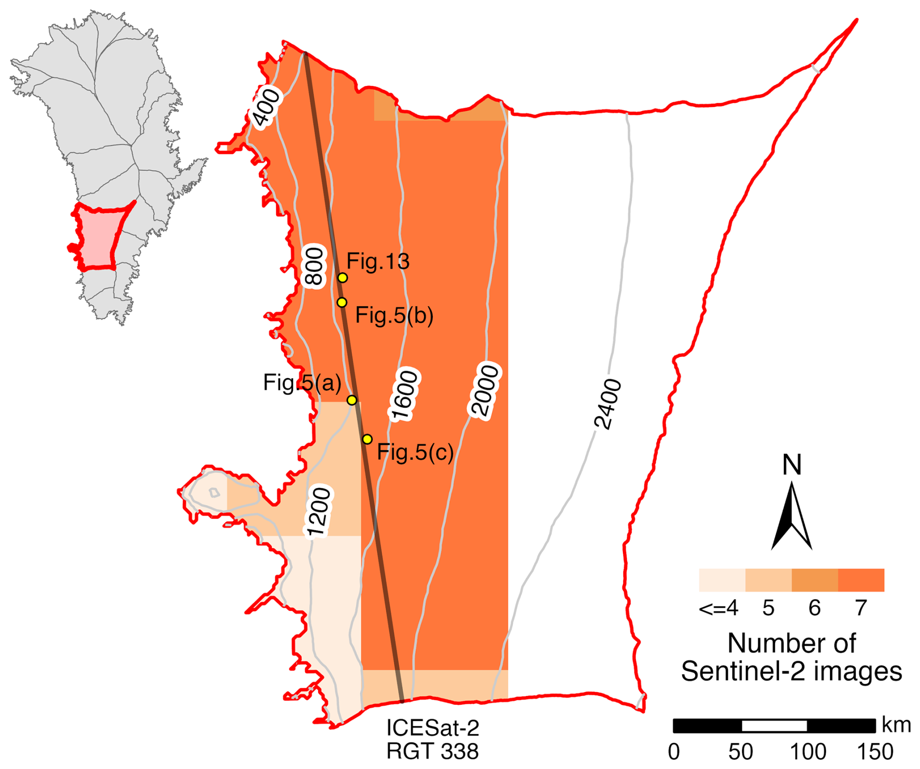
Figure 1 Study area. Contour lines calculated from ArcticDEM mosaic version 4.1 (Porter et al., 2023) are visible as grey lines at 400 m intervals. Yellow points indicate the locations of the lakes in the study area, as shown in Figs. 5 and 13. The study period is from June to August 2022.

2.2 Sentinel-2 imagery

Sentinel-2 consists of two polar-orbiting satellites (Sentinel-2A and Sentinel-2B), which provides a revisit cycle of about 5 d. The MultiSpectral Instrument (MSI), a push-broom optical sensor on board Sentinel-2, can collect data in 13 spectral bands. Using the significant attenuation characteristics of light in water, four bands with a spatial resolution of 10 m are used in this study, specifically the three visible light bands (blue band with a center wavelength of 0.49 µm, green band with a center wavelength of 0.56 µm, and red band with a center wavelength of 0.665 µm) and one near-infrared (NIR) band with a center wavelength of 0.842 µm. Considering that SGLs only form below the equilibrium line altitude, only images covering areas below 2000 m within the basin are selected. To minimize the effect of cloud cover, we limit the cloud cover when selecting the images. In this study, we use a total of 81 images, 53 of which have 0 % cloud cover. Among the remaining 28 images, only one has a cloud coverage rate of 11.09 %, while the others exhibit minimal cloud coverage, with an average of 1.62 %. During the whole melt season, when the SGLs of Greenland undergo the most pronounced changes, a total of 81 Sentinel-2 level-1C images (orthocorrected and geometrically corrected top-of-atmosphere (TOA) reflectance products) divided into 7 periods, with a period of approximately 10 d between observations, are included in this study, covering the study area from 7 June to 28 August 2022. It should be noted that no single day's imagery could cover the entire study area during the second and third study periods (i.e., 15–20 June and 30 June–4 July). Therefore, we use multiple images from different days to achieve complete coverage of the study area, denoted by 17 June and 2 July to represent these two periods in the following text. For overlapping regions from different dates, each individual image is processed separately, and the final result is obtained by averaging the processed outcomes.

2.3 ICESat-2

ICESat-2 was launched by the National Aeronautics and Space Administration (NASA) in September 2018 with polar exploration as its primary objective. In achieving this objective, it can provide elevations of sea ice, land ice, and water height amongst other data (Neumann et al., 2021). Equipped with the advanced topographic laser altimeter system (ATLAS), it is capable of transmitting laser pulses with a wavelength of 532 nm at a repetition frequency of 10 kHz. ATLAS employs three pairs of laser pulses, with each pair separated by approximately 3 km in the cross-track direction. The satellite acquires overlapping light spots with an interval of approximately 0.7 m and a diameter of approximately 17 m along its orbit with a 91 d revisiting cycle (Neumann et al., 2021).

In this study, strong beams in each pair of laser pulses are selected. The ATLAS version 3 (ATL03) product provides photon data of surface elevation with latitude and longitude coordinates using the WGS84 reference ellipsoid with a spatial resolution of 0.1 and 0.7 m in horizontal and vertical directions, respectively, which is mainly used to extract the depth of the SGLs. The ATLAS version 6 (ATL06) surface elevation product at a coarser spatial resolution is used during the preprocessing step to exclude significant height noise. Both ATL03 and ATL06 products are downloaded through the National Snow and Ice Data Center website (https://nsidc.org/data/icesat-2, last access: 11 July 2025). Considering the changes in SGLs, it is important to minimize the temporal difference between ICESat-2 data and Sentinel-2 images. Therefore, the ATL03 product and the corresponding ATL06 product acquired from the orbit of the reference ground track (RGT) no. 338 on 14 July 2022 are used in this study, since it is the only day during the entire melt season of 2022 when both ICESat-2 data and Sentinel-2 images are available. Then, both ICESat-2 data and Sentinel-2 images are converted to the UTM zone 22N (EPSG:32622) for further analysis.

3 Methods

The proposed framework for the inversion of SGLs, as shown in Fig. 2, consists of three modules: extraction of SGLs using Sentinel-2 imagery, detection of SGL depths on the ICESat-2 RGT, and inversion of the entire lake depths using an MLP model.

Figure 2 Framework of the proposed SGL depth inversion method.

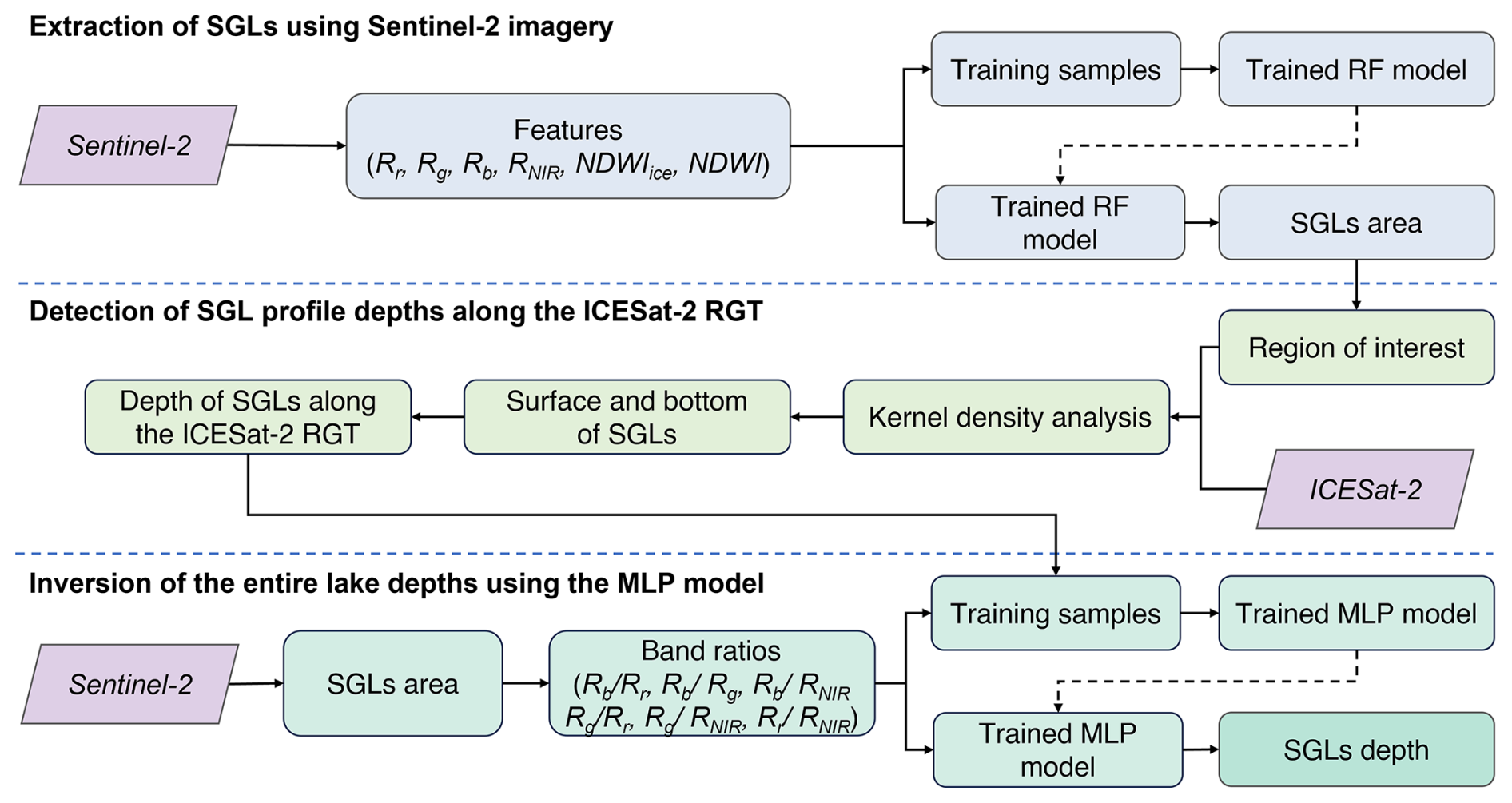
3.1 Extraction of SGLs using Sentinel-2 imagery

The RF model, an ensemble learning method composed of multiple independently trained decision trees, is utilized to extract the lakes based on the spectral features. The advantage of the RF model is its ability to reduce the risk of overfitting by constructing decision trees using randomly selected samples and features (Breiman, 2001). The final prediction result of an RF is based on the majority vote from all decision trees since each decision tree is independent and complements each other. For feature selection, in addition to the reflection values of the red, green, blue, and NIR bands, NDWI_ice and NDWI are also included, considering the unique icy and snowy environment of SGLs. The calculations for NDWI_ice and NDWI are shown in Eqs. (1) and (2), where R_r, R_g, R_b, and R_NIR represent the reflection values of the red, green, blue, and near-infrared bands, respectively.

$$\begin{array}{}\text{(1)}& {\displaystyle }{\mathrm{NDWI}}_{\mathrm{ice}}={\displaystyle \frac{R_{\mathrm{b}}-R_{\mathrm{r}}}{R_{\mathrm{b}}+R_{\mathrm{r}}}}\text{(2)}& {\displaystyle }\mathrm{NDWI}={\displaystyle \frac{R_{\mathrm{g}}-R_{\mathrm{NIR}}}{R_{\mathrm{g}}+R_{\mathrm{NIR}}}}\end{array}$$

For each time period, we randomly sample 50 pixels from SGL areas and 50 pixels from other areas in the mosaicked Sentinel-2 image as training data and then employ an RF algorithm with 30 decision trees to classify the image into lake and non-lake. The trained model is then applied to Sentinel-2 images of seven periods in the study area to extract SGLs. All the Sentinel-2 image processing tasks are conducted on the Google Earth Engine (GEE) platform.

3.2 Detection of SGL profile depths along the ICESat-2 RGT

The regions of interest in the ICESat-2 data are identified based on the extraction results of SGLs from the Sentinel-2 image. To ensure that the altimetry data further processed include both data inside and outside the lake, we establish a 100 m buffer zone around each SGL. Windows based on ATL06 surface elevation data establish the vertical extent of the ATL03 photon data used, while buffer zones determine the range of data along the track direction. Then, the kernel density analysis method is employed to discern the surface and bottom of the lake from the multiple reflections of ATL03 photons on the various surfaces of the SGL. Subsequently, the precise boundary of the SGL is determined according to the breakpoints of the surface slope change. Considering that the surface of the ice sheet has a more pronounced topographic undulation, while the SGL is water surface and therefore horizontal, the extent of the SGL is determined by detecting the slope change of the surface. Within this precise boundary of the SGL, a refraction correction (Parrish et al., 2019) is applied to determine the actual depth of each SGL. The most reliable method to assess the uncertainty in depth oriented from ICESat-2 data is by comparing inversion results with in situ measurements. However, due to the harsh environment in Greenland and the rapid changes of SGLs during the melting season, obtaining in situ data near the ICESat-2 transit time is challenging. In this study, the quality of depth data derived from ICESat-2 is ensured through visual inspection, and the profile depth extracted from ICESat-2 ATL03 data is the reference for the Sentinel-2 depth estimation.

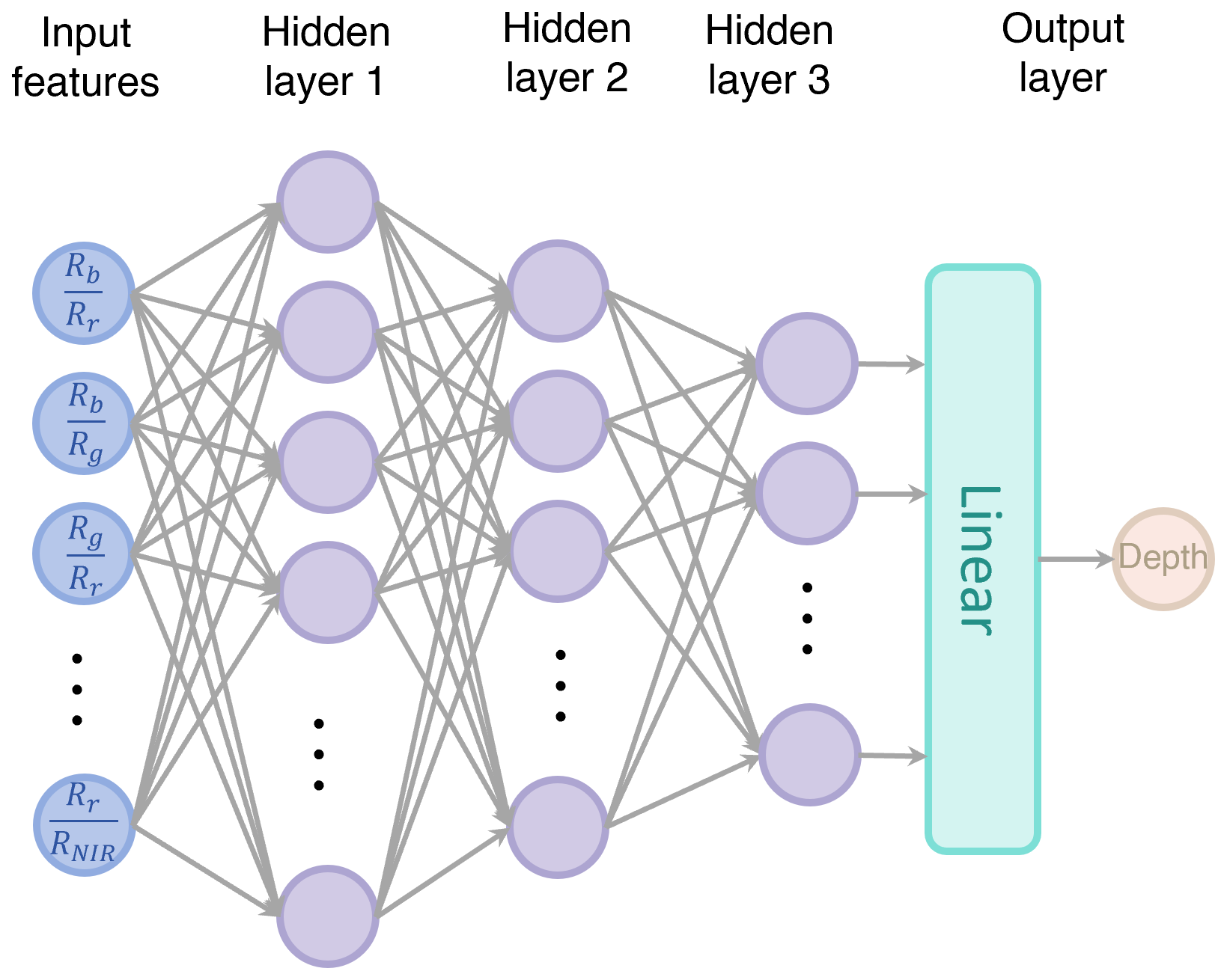
3.3 Inversion of the entire lake depths using the MLP model

Considering the discrepancy in spatial resolution between the depth estimates obtained by ICESat-2 data and the Sentinel-2 imagery, we create a dataset by computing the average depth value from the output of ICESat-2 ATL03 data within a Sentinel-2 pixel. Inspired by Lai et al. (2022) on optical shallow water depth inversion in mid- and low-latitude regions, we construct an MLP architecture consisting of three hidden layers (Fig. 3): the first with 128 nodes, the second with 32 nodes, and the third with 16 nodes. The three hidden layers are connected using the rectified linear unit (ReLU) activation function. A linear activation function is applied to the output layer, which provides depth estimates corresponding to each pixel. The depth of the SGL exhibits a non-linear relationship with the ratio of reflectance between blue and red bands (Legleiter et al., 2014). Motivated by this insight, we opt for a more comprehensive approach by considering multiple band ratios, specifically the top-of-atmosphere (TOA) reflectance ratios between the red, green, blue, and near-infrared bands, derived from Sentinel-2 imagery, as input features for the MLP. Both the depth of SGLs from two pairs of ICESat-2 RGT no. 338 and the corresponding band ratios within SGL areas from Sentinel-2 images are used to train the MLP model, and the data in the remaining pair of ICESat-2 RGT no. 338 are used to test the performance of the MLP model. Then, the trained MLP model is applied to invert the depth of SGLs within seven time periods across the whole study area.

Figure 3 Structure of the MLP model.

3.4 Evaluation methods

To quantitatively evaluate the performance of the classification algorithm, the intersection over union (IoU) metric is used, which is the proportion of the overlap between the classification results and manually selected SGLs relative to their combined area. To evaluate the performance on depth prediction, we compare the effectiveness of both MLP model and the empirical formula approach (Box and Ski, 2007). The empirical formula approach establishes an empirical relationship between SGL reflectance and depth as shown in Eq. (3). The same training and testing data are adopted, allowing for a comparison of the performance between MLP and the empirical formula method.

$$\begin{array}{}\text{(3)}& D={\displaystyle \frac{{\mathit{\alpha }}_{\mathrm{0}}}{R+{\mathit{\alpha }}_{\mathrm{1}}}}+{\mathit{\alpha }}_{\mathrm{2}},\end{array}$$

where D represents the estimated depth of the SGL. R denotes the reflectance in the green or red band, and parameters α₀, α₁, and α₂ are empirical coefficients fitted by using training data.

The mean absolute error (MAE) is adopted to assess the depth inversion accuracy of both the MLP model and the empirical formula method. The calculation method for MAE r_mean is

$$\begin{array}{}\text{(4)}& r_{\mathrm{mean}}={\displaystyle \frac{\sum |d_{\mathrm{ref}}-d_{\mathrm{pred}}|}{N}},\end{array}$$

where d_ref represents the lake depth obtained by ICESat-2, d_pred represents the predicted lake depth value using the MLP model or empirical formula method, and N is the number of pixels.

4 Results

4.1 Evaluation of area extraction and depth inversion

We manually selected five SGLs on each image, compare them with the RF extraction results, as shown in Fig. 4, and calculate the IoU value for each image. The results are shown in Table 1. The difference between the manually selected continuous boundaries and the jagged edges on raster images significantly affects the accuracy of image IoU. This effect is particularly noticeable during the early melting stages (i.e., 7 June) of the SGLs since the area of the SGLs is relatively small. As the melting intensifies and the SGL area increases, the impact of this difference on IoU evaluation decreases in subsequent results, with all IoU values remaining around 90 %. Overall, the average IoU value for the SGLs across seven periods is 90.20 %, providing reliable SGL extents for subsequent experiments.

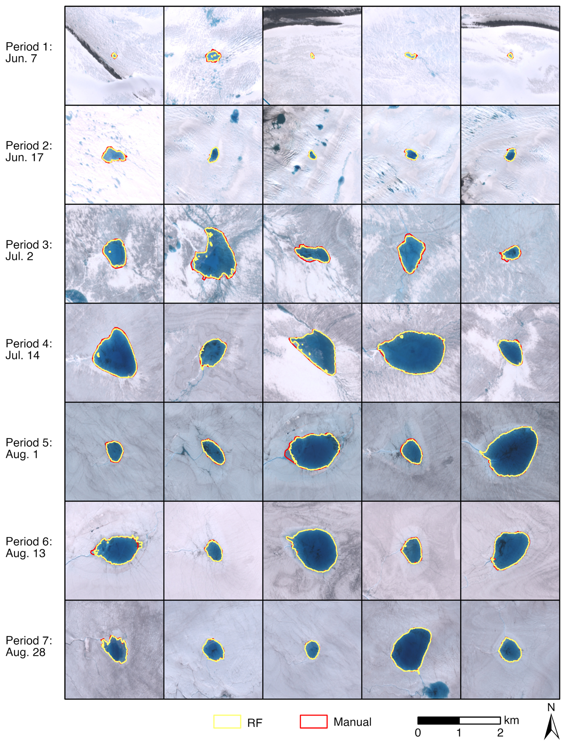
Figure 4 The comparison between the extracted extents and manually delineated contours for five different SGLs randomly selected from each study period, using the corresponding Sentinel-2 images as a background for each period. Each row represents a different time period.

Table 1 Accuracy assessment of extraction results of SGLs showing the intersection over union (IoU) of each time period's SGLs.

The detection results of the lake surface and bottom are shown in Fig. 5; the difference between the two represents the lake's depth. The detected lake depth based on ICESat-2 data is considered the reference in this paper since the reliability of this method has been verified (Lutz et al., 2024; Melling et al., 2024). In the study area, there are a total of 1991 pixels over 28 SGLs in Sentinel-2 imagery, which coincide with three laser beams (gt1l, gt2l, gt3l) of ICESat-2 RGT no. 338. Among them, 994 pixels are used as training samples for the MLP training, while the remaining are used for evaluating the accuracy of MLP inversion results for lake depth.

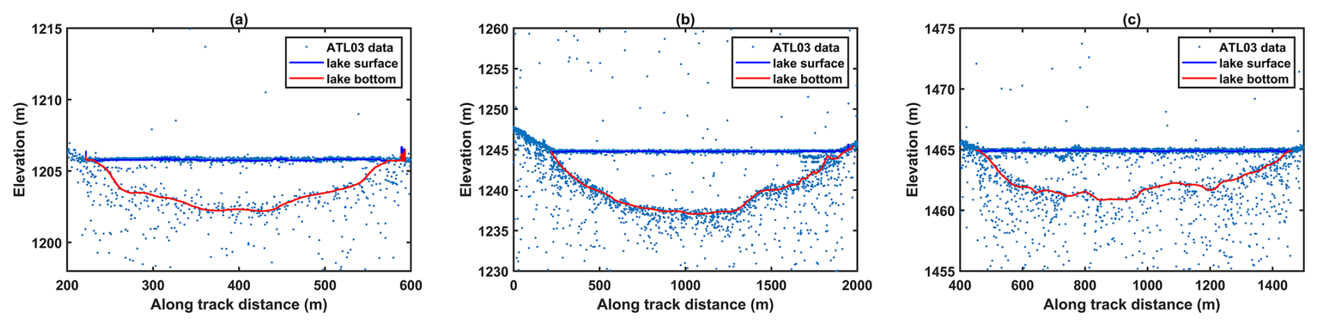
Figure 5 Panels (a), (b), and (c) show three examples of lake surface and bottom detection results based on ICESat-2 ATL03 data. The locations of these three lakes are shown in Fig. 1.

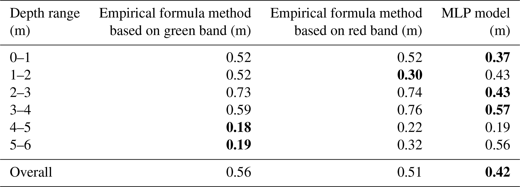
The comparison of the depth inversion accuracy for both the empirical formula method and the MLP model over different depths is presented in Table 2, where the results in bold indicate the highest accuracy in the depth inversion. Although the results based on the empirical formula method demonstrate superiority in predicting depths within the ranges of 1–2 and 4–6 m, the MLP model exhibits an overall MAE of 0.42 m across all depth ranges, significantly outperforming the empirical formula method. The advantage of the MLP model lies in its ability to leverage multiple inputs for feature selection, which integrates more band information and can fully utilize the information of different bands in the image compared to the single-band inversion of the empirical formula method, thus achieving higher-accuracy results.

Table 2 MAE of lake depth inversed by the empirical formula method and the MLP model at different depths, where the results in bold indicate the highest accuracy for each depth range.

To analyze the distribution of the depth inversion errors, we plot depth inversion bias maps and assign different colors based on the point density (Fig. 6). The depth inversion bias distribution of the MLP method is closer to the horizontal axis compared to that of the empirical formula method, while the depth inversion results obtained by the empirical formula method almost always have a linear bias. Within the 1–2 m range, the intersection of the linear bias predicted by the red band with the horizontal axis partly explains why the empirical formula method achieves the highest accuracy in this depth interval.

Unlike a physically based depth inversion method, the MLP model learns the relationship between lake depth and input features through training data. Therefore, issues such as the data quality of the dataset and the uneven distribution of the number of data samples at each depth will greatly affect the inversion results of the MLP. As can be seen from Fig. 6, the number of sample points at depths above 3 m is significantly less than the number of sample points at depths below 3 m, with the lowest number of points at the 5–6 m depth interval. The combination of the above reasons leads to the inversion results of the MLP model at 5–6 m being inferior to the inversion results of the empirical formula method.

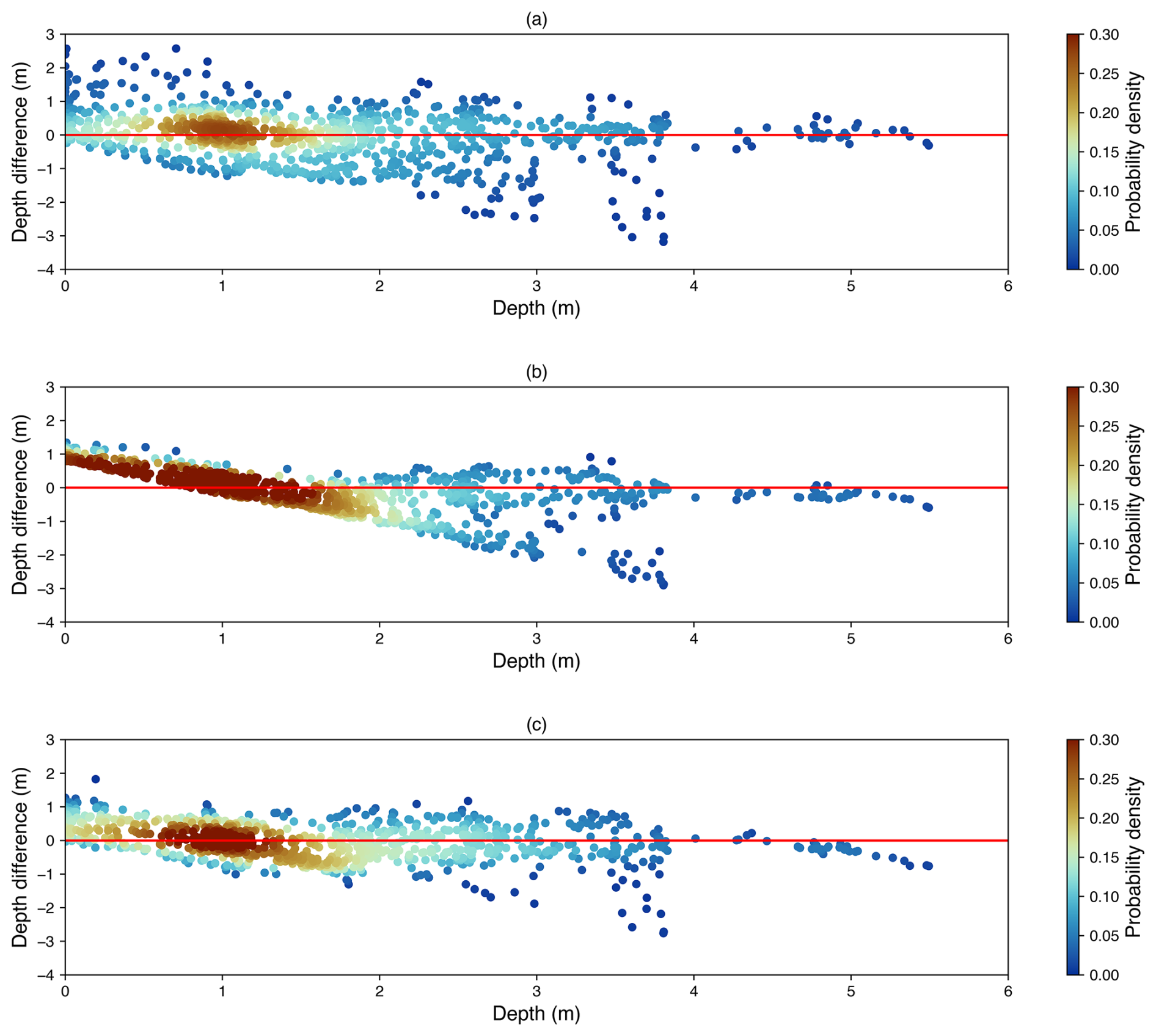
Figure 6 The depth inversion bias maps obtained by the empirical formula method based on the green (a) or red (b) band and the MLP model (c). Each point in each of the plots corresponds to an SGL pixel.

4.2 The spatiotemporal variation characteristics of SGL parameters during the 2022 melt season

The results of the SGL area extraction and depth inversion over our studied time periods are depicted in Fig. 7. The spatial and temporal distribution of SGLs extracted at different periods shows significant variation. During the entire melt season, SGLs appear at different elevation ranges at different stages, with varying areas and depths. On 7 and 17 June, the SGLs primarily distribute in the coastal areas around and below an elevation of 800 m (Fig. 7a). However, the SGLs on 7 June are smaller in area and shallower in depth, with no significant large lakes. By 17 June, the area and depth of the SGLs have increased, and notable lakes appear near the 800 m contour line (Figs. 7b, 8a). In contrast, the SGLs on 2 July show significant differences from the previous two periods, primarily occupying the 800 to 1200 m region, with noticeable increases in area and depth (Figs. 7c, 8a, b). SGLs larger than 3 × 10⁶ m² begin to appear (red outlines in Fig. 7c). On 14 July, the SGLs further advance to higher elevations, extensively distributed between 800 and 1600 m (Fig. 7d). The area and depth of the SGLs continue to grow, with several large lakes around the 1200 m contour line (Fig. 8b). The number of lakes larger than 3 × 10⁶ m² increases from one to three (red outlines in Fig. 7d). On 1 August, the trend in SGLs advancing to higher elevations slows, with most SGLs distributed between 1200 and 1600 m (Fig. 7e). The overall area and volume slightly increase, with the number of lakes larger than 3 × 10⁶ m² reaching nine (red outlines in Fig. 7e). By 13 August, the SGLs do not continue to expand to higher elevations, mainly occupying the 1200 to 1600 m range (Fig. 7f). As the melt season approaches its end, some SGLs are covered by snow and ice, reducing their numbers. However, large and deep SGLs are still around the 1600 m contour line (Fig. 8c). On 28 August, the number of SGLs significantly decreases, showing some variation in spatial distribution (Fig. 7g). A few deep and large lakes remain above 1200 m, while more shallow and small SGLs appear in coastal areas below 800 m.

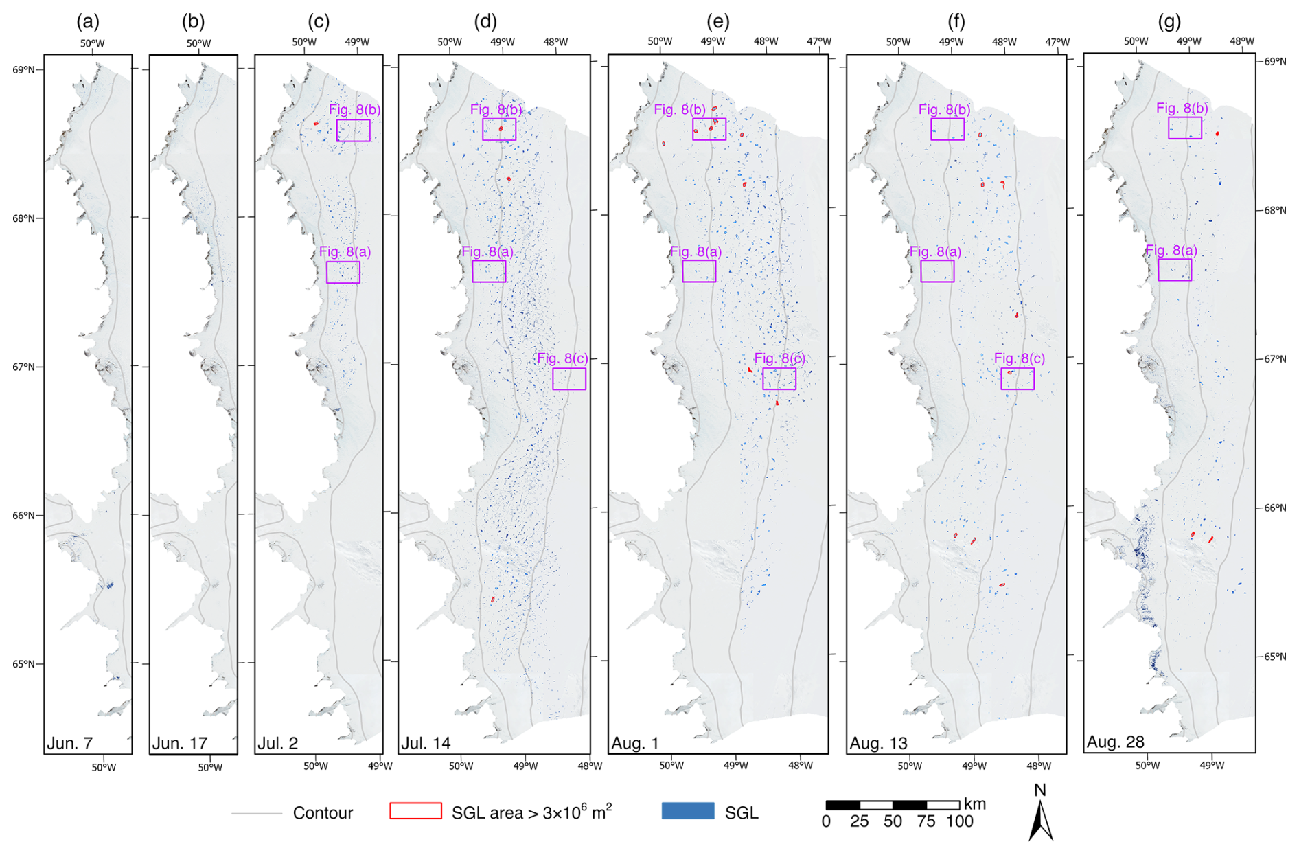
Figure 7 SGL area extraction and depth inversion results on 7 June (a), 17 June (b), 2 July (c), 14 July (d), 1 August (e), 13 August (f), and 28 August (g). The background map is Sentinel-2 images from each respective period. Contour lines from ArcticDEM mosaic version 4.1 (Porter et al., 2023) are also shown in grey at 400 m intervals.

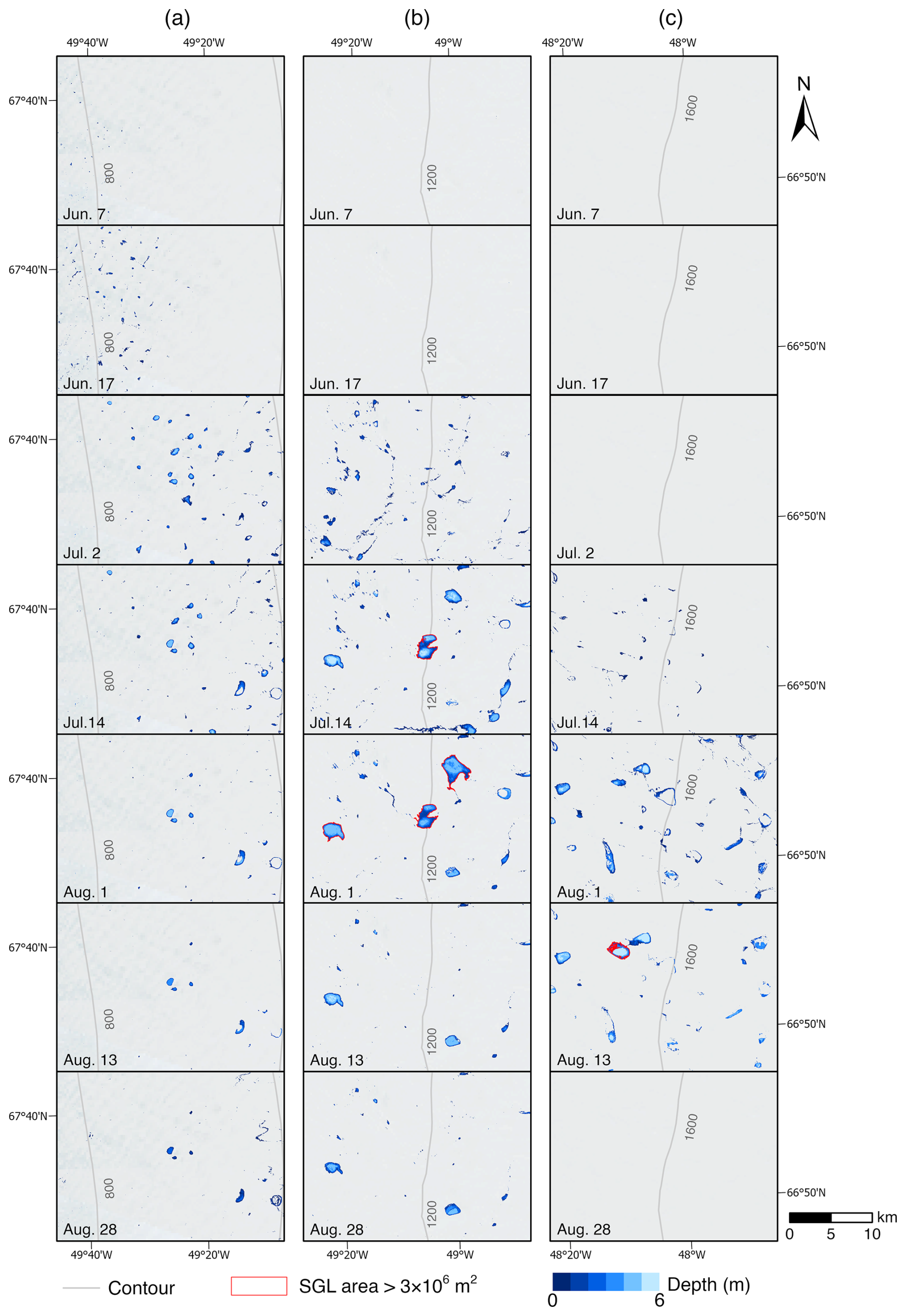
Figure 8 Zoomed-in view of the evolution of SGL area and depth at elevations of around 800 m (a), 1200 m (b), and 1600 m (c). The background map is Sentinel-2 images from each respective period. Contour lines from ArcticDEM mosaic version 4.1 (Porter et al., 2023) are also shown in grey at 400 m intervals.

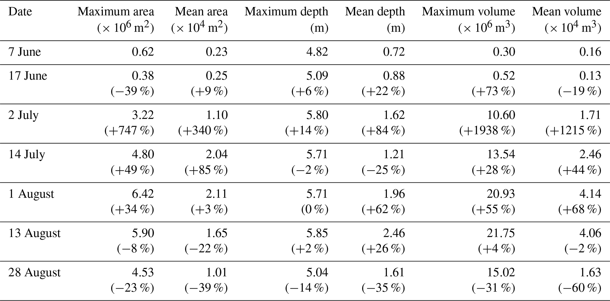
To mitigate the impact of differences in the number of available images across different periods, the maximum and average values of area, depth, and volume of the SGLs are compared in Table 3. At the beginning of the development of the SGLs (7–17 June), due to the relatively small amount of melting, there are a number of small areas of water on the edge of the ice sheet. At this time, the area and volume of each individual SGL are relatively small, measuring less than 1 × 10⁶ m² and 1 × 10⁶ m³, respectively, with a mean depth of less than 1 m. Afterward, the SGLs enter a period of rapid melting, where the maximum area of the individual lake increases from 0.38 × 10⁶ to 3.22 × 10⁶ m² with a growth rate of +747 % from 17 June to 2 July, and the maximum volume of the SGL increases from 0.52 × 10⁶ to 10.60 × 10⁶ m³ with a growth rate of +1938 %. Similarly, the average area, depth, and volume increase rapidly with a growth rate of +340 %, +84 %, and +1215 %, respectively, which is significantly different from the previous period and implies that the SGL had begun to enter the peak of its development as the melt season progressed.

After entering the peak period of development, the maximum and mean area of the SGLs show a sustained upward trend between 2 and 14 July, with a growth rate of +49 % and +85 %, respectively. However, the maximum and mean depth show decreasing trends. Overall, the maximum and mean volume of the SGLs show an increasing trend, with rises of +28 % and +44 %, respectively. The growth rate of the area of the SGLs is higher than the growth rate of the volume, indicating that a large number of large and shallower-depth SGLs appeared during this period. Then, the mean area and volume of the SGLs reach the maximum on 1 August, with the growth rate of +3 % and +68 %, respectively, indicating that the mean area of the SGLs has already stabilized at that time, while the mean volume is still in the stage of high-speed growth. On 13 August, although the depth of SGLs continues to increase, the area shows a significant decreasing trend, resulting in the volume remaining comparable to that on 1 August. Between 13 and 28 August, the maximum and mean values of areas, depth, and volume of SGLs show a decreasing trend, indicating that the lakes begin to recede as time progresses toward the end of the melt season. And the rate of decline of the mean values of the SGLs (−39 %) exceeds that of maximum values (−23 %), indicating that most of the SGLs are frozen or drained overall, but there are a few lakes with large areas and volumes of water that still existed.

Table 3 Statistics of the maximum and mean values of the SGL area, depth, and volume for the seven study periods, with the growth rate against the previous period given in parentheses.

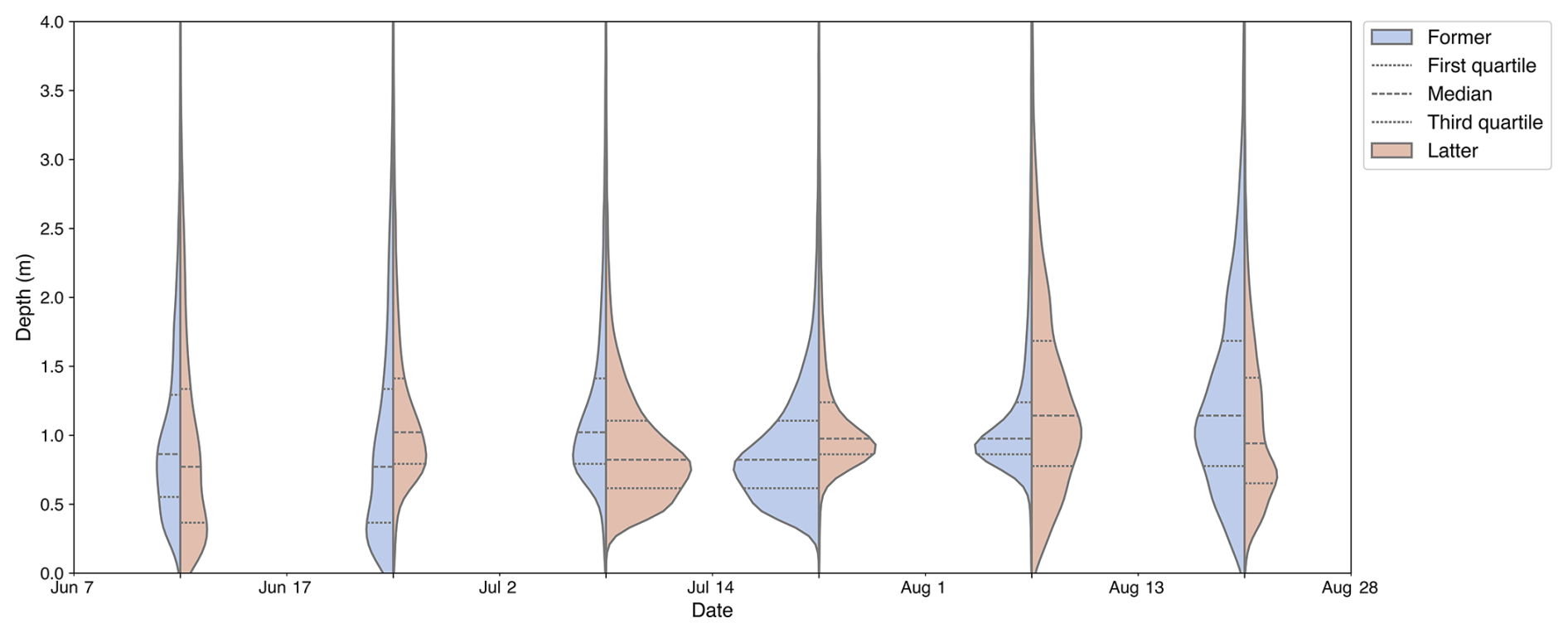
The depth distribution of SGLs in each period is plotted as a violin plot (Fig. 9), ignoring lakes above 4 m, which accounted for less than 2 % of the total. To demonstrate the difference in distribution between the two adjacent periods, we differentiate the violin plots of the previous time (blue) and the later time (brown) by color; i.e., the distribution of the statistical plots on the remaining time except the first and last time is compared with its previous and subsequent periods, respectively. The major difference is between the 17 June and 2 July plots, where the peak position clearly shifts upward, and the distribution of depth data between the upper and lower quartiles is more concentrated; i.e., the depth of the SGL begins to develop more steadily on the existing base rather than melting randomly, corresponding to the transition from the early to the peak period of SGL development. Subsequently, the distribution of maximum depths during the peak period of SGL development is relatively concentrated with obvious peaks, while the median is similar to the trend in average depths, also appearing to decrease and then increase, indicating that more shallow SGLs are formed during 2 to 14 July. The median peak on 1 August shows the most concentrated distribution shape of all periods, suggesting that the development of SGLs has reached a relative peak and that the maximum depth has stabilized. The subsequent distribution on 13 August differs significantly from that of 1 August. Although the median value still increases, there is no longer a prominent peak, and the upper and lower quartiles show obvious dispersion. The increase in the median value indicates that some deeper SGLs still exist, but the overall dispersion of the data still indicates that the development of SGLs has entered a period of decline, and the distribution of maximum depths on 28 August is more toward shallower water.

Figure 9 Violin plots of SGL depth distribution over our seven study periods.

A density map of the distribution of the area of each SGL and its corresponding average depth over different time periods is created to further examine the distribution and changes in area and depth of SGLs over the melting seasons. For better display of figures, only the SGLs with an area less than 5 × 10⁴ m² and an average depth below 3 m, which covers more than 90 % of the SGLs within each period, are shown in Fig. 10. Each data point on the density map represents a single SGL, and brighter colors indicate higher density, corresponding to a greater number of SGLs.

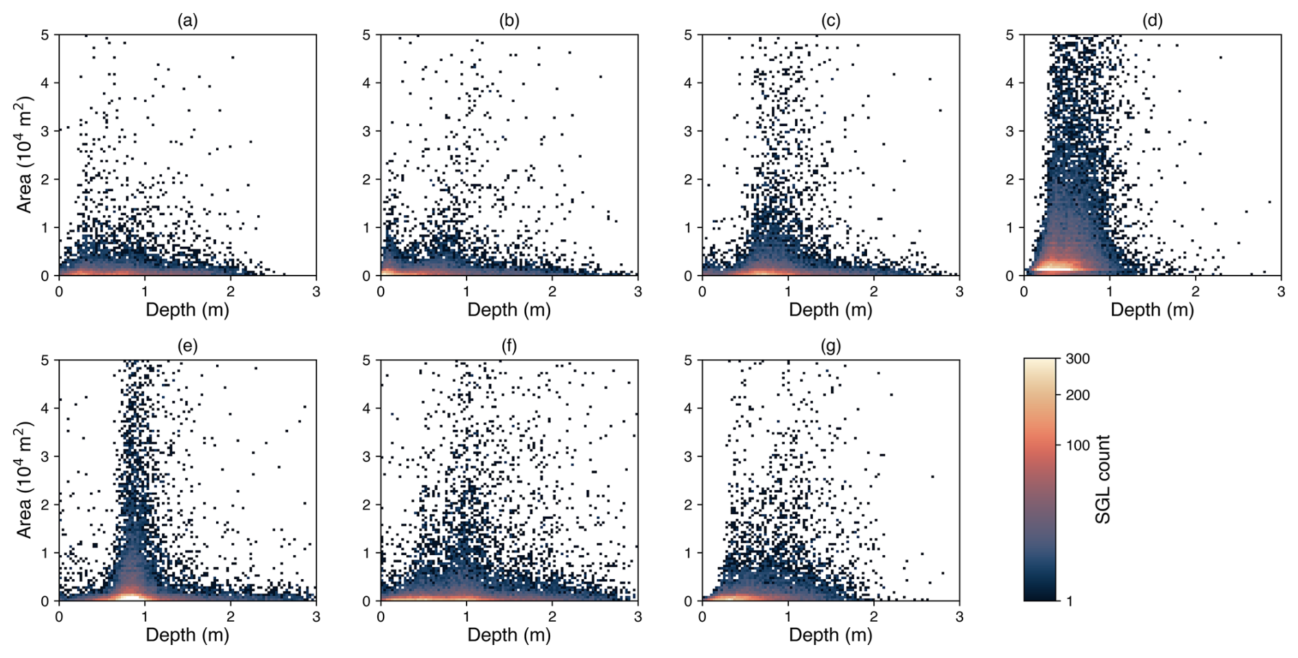
Figure 10 The area–depth distribution map of each individual SGLs on 7 June (a), 17 June (b), 2 July (c), 14 July (d), 1 August (e), 13 August (f), and 28 August (g).

The distribution of SGLs across all periods exhibits a clear trend from scattered to concentrated and then back to scattered. During the initial development phase (as seen in Fig. 10a, b), the brighter regions cluster near the origin, indicating a higher abundance of small and shallow SGLs. Beginning with 2 July, a distinct peak appears, with SGL depths gradually concentrating between 0.5 and 1 m, as shown in Fig. 10c. By 14 July, the number of SGLs increases significantly. A significant portion of these lakes have an average depth distribution in the range of 0.2 to 1 m, with a pronounced peak near 0.3 m, as indicated in Fig. 10d. In addition, there is a notable increase in the number of SGLs with areas greater than 2 × 10⁴ m² and relatively shallow depths. This observation is consistent with the overall decrease in mean depth during the development of SGLs as shown in Table 3. On 1 August, the distribution of SGLs becomes more concentrated. The brighter regions shift to deeper mean depths, reaching about 0.8 m, as presented in Fig. 10e. Many SGLs now have mean depths of around 0.9 m. Compared to 14 July, there is a significant increase in the number of SGLs with mean depths exceeding 2 m. By 13 August, the distinct peak diminishes, and the distribution of SGLs is no longer concentrated around a single point. Instead, it gradually spreads out, as shown in Fig. 10f. The number of lakes with average depths greater than 2 m continues to increase. At this stage, SGLs show variability; i.e., some evolve into larger, deeper lakes, while others retreat into smaller, shallower lakes. This characteristic marks the transition to the late stage of development. Even within small regions, individual SGLs show significant variation. Within the same area, some lakes may grow larger, while others may freeze or drain (as shown in the fifth and sixth rows in Fig. 7c). During the late stage of SGL development, extensive drainage or freezing leads to reductions in area, depth, and the total number of lakes, as shown in Fig. 10g. The brighter regions converge to smaller areas and shallower depths, and the number of SGLs with average depths greater than 2 m rapidly decreases.

Finally, Fig. 11 illustrates the volume distributions and the total volume of SGLs at each of the seven periods. The boxplots encapsulate the interquartile range (IQR), with the median volumes denoted by red lines within the turquoise boxes, and the whiskers extending to 1.5 times the IQR. Outliers, which are defined as the first and the last 1 % of the data, are indicated by grey points, while the red triangles connected by a dotted line represent the mean volumes. Throughout the observation period, the median volume of the SGLs exhibits minor fluctuations; the largest median volume is on 14 July, which is around 10 m³. Conversely, the mean volumes show a discernible increasing trend from early June, peaking on 1 August, before slightly declining towards the end of August. This divergence between the median and mean suggests that while the majority of lakes maintain stable volumes, a subset of lakes experience significant volume increases, thus elevating the mean. The persistent presence of high-volume outliers across all dates further corroborates this observation, indicating the existence of lakes with substantially larger volumes compared to the majority. The consistency in the volume range and outliers underscores the dynamic nature of supraglacial lakes, likely influenced by varying melting rates, precipitation, and drainage patterns. This analysis highlights the complex behavior of supraglacial lake volumes over the summer months, with a few lakes significantly impacting the overall mean despite the general stability in median volumes. Meanwhile, the total volume of the SGLs during the seven study periods is also presented by the blue line in Fig. 11. Starting from 2 July, the total volume of the SGLs shows a sharp increase, reaching its maximum value of 9.30 × 10⁸ m³ on 1 August. Afterward, the volume of the SGLs begins to decrease until the end of August.

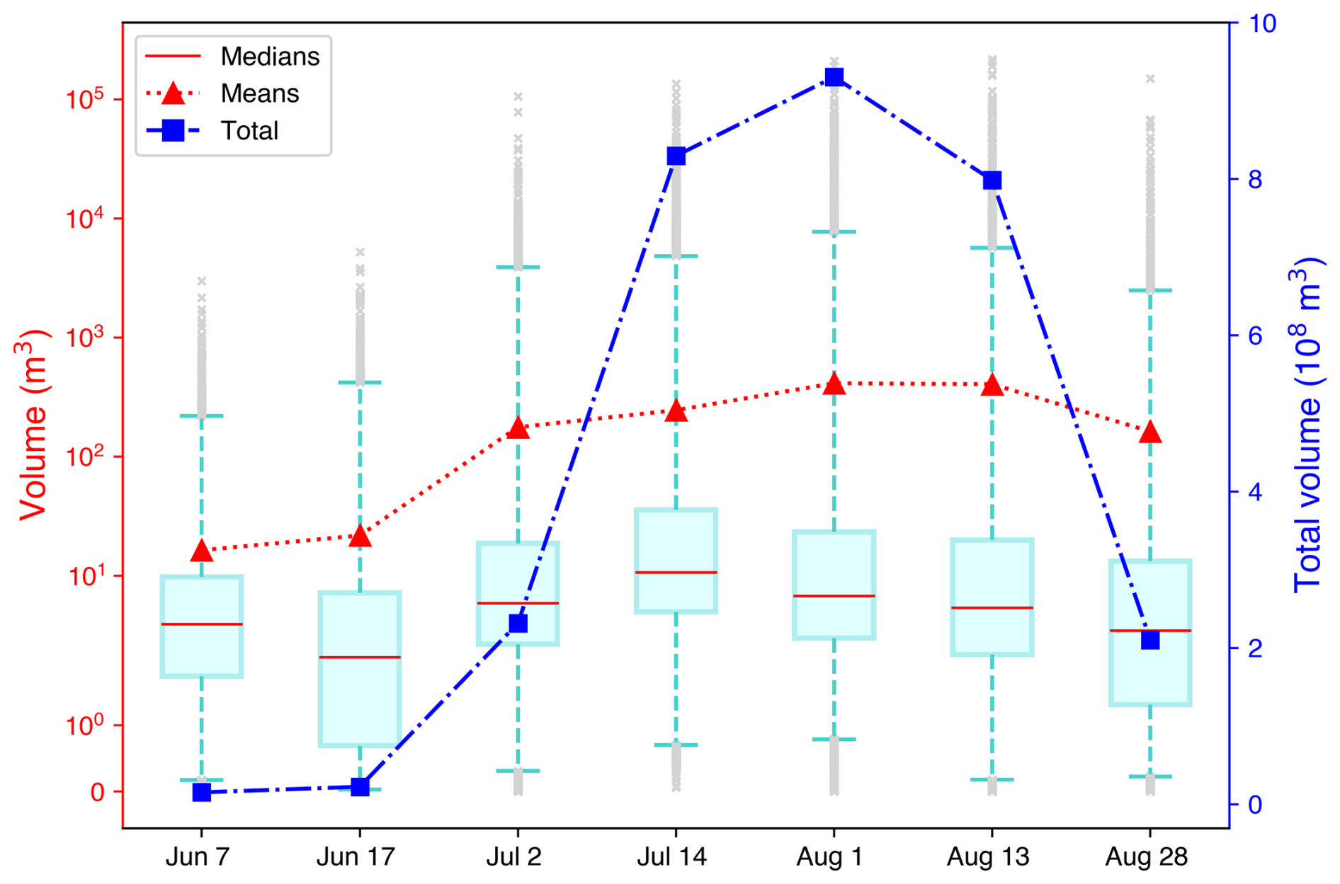
Figure 11 Boxplots of each individual SGL volume and the total volume during the seven study periods.

4.3 The evolution characteristics of SGLs at different elevations

To further analyze the spatial distribution of SGL development in relation to elevation, we divide the elevation range from 0 to 2000 m into five intervals of 400 m each and calculated the average area, depth, and volume of SGLs within each interval. Figure 12 illustrates these statistics, with colors representing elevation from light to dark, grey dashed lines indicating the overall average, and red stars marking the maximum values for each line.

Figure 12 SGL average area (a), depth (b), and volume (c) at different elevation intervals.

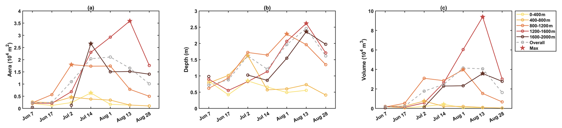
Generally, there is a significant difference between SGLs above and below 800 m. The average area, depth, and volume of SGLs below 800 m remain relatively stable with minimal fluctuations. In contrast, SGLs above 800 m exhibit more variability and dominate the overall trends of various statistics. The most drastic changes in area, depth, and volume occur between 1200 and 1600 m, indicating this elevation range is the most favorable for SGL formation.

According to the average area at different elevations (shown in Fig. 12a), the overall peak area is reached around early August, specifically on 1 August, driven primarily by lakes in the 1200–1600 m range, with the highest value recorded at 3.5 × 10⁴ m² on 13 August. Each elevation band shows a similar trend with varying magnitudes, peaking mostly between late July and early August, suggesting mid-summer as the period of maximum lake expansion. After 14 July, the area of SGLs between 1200 and 1600 m continues to increase until peaking on 13 August and then decreases, while the average area of SGLs above 1600 m decreases and then stabilizes.

Figure 12b presents the average depth of SGLs across different elevations. Peaks in mean depths for the 0–400 and 400–800 m ranges occurred on 2 July, with mean depths in the 400–800 m range significantly higher than those in the 0–400 m range. Before 2 July, the overall mean depth change is dominated by SGLs between 400 and 1200 m. After 2 July, the mean depth change is dominated by SGLs above 800 m. Mean depths in all elevation segments decrease between 2 and 14 July, except for those between 1200 and 1600 m. Between 14 July and 1 August, the mean depths of SGLs above 800 m increase rapidly, creating a more pronounced difference with those below 800 m, with mean depths in the 800–1200 m range reaching a peak. From 1 to 13 August, the mean depth of SGLs above 1200 m continue to increase, albeit at a slower rate, reaching its maximum mean depth on 13 August, while the mean depth of SGLs between 800 and 1200 m begin to decrease. After 13 August, the mean depth of SGLs decreases across all elevation bands as the ablation season approached its end.

The average volume of SGLs in different elevation zones generally follows a trend of increasing and then decreasing, with the exception of SGLs between 800 and 1200 m, which show a smaller decrease on 2 July and then increase again (as shown in Fig. 12c). The higher the elevation of the SGL, the later its average volume reaches its peak, reflecting the spatial distribution of SGLs. As the melt season advances, SGLs gradually push inland from the coast, reaching elevations of 1800 m or higher. The volume change of SGLs between 1200 and 1600 m is particularly notable, with the peak average volume significantly larger than that of other elevation intervals. This is due to the cumulative advantage of depth and area, making the probability of large and deep lakes significantly higher in this elevation interval compared to others.

In summary, the elevation range of 1200–1600 m is the most conducive for the development of SGLs, with significant changes in area, depth, and volume, especially during the mid-summer peak. This range sees the most substantial lake formation and expansion, with the highest occurrence of large and deep lakes.

5 Discussion

5.1 The uncertainty in SGL depth inversion

The presence of ice and snow cover on the surface of SGLs significantly influences the reliability of depth inversion. As shown in Fig. 13a, a distinct SGL is partially covered with ice or snow. The ICESat-2 track passes over this lake and the covered areas. In the segment from P₂ to P₃, the Sentinel-2 image provides band reflection information from the ice surface. This situation presents a significant challenge for both the empirical formula method and the MLP method. As shown in Fig. 13c, depth measurement methods relying on optical images face obstructions in this segment, leading to an abrupt change in depth and a significant underestimation of depth in ice/snow-covered areas. As for ICESat-2 data, the sparse bathymetric photons, influenced by ice or snow in this segment, as shown in Fig. 13b, complicates the depth measurements. Although fitting a continuous bottom (red line in Fig. 13b) makes the depth results appear more reasonable, using interpolated depth as a reference does not provide an accurate evaluation of the empirical formula method and the MLP model. Therefore, we manually remove this type of segments to ensure the reliability of depth from ICESat-2 data. In the segment from P₃ to P₄, although the lake surface is covered by floating ice, the MLP-based depth inversion method can partially overcome this impact. This improves the estimation of lake depth, providing results closer to those obtained using ICESat-2 data.

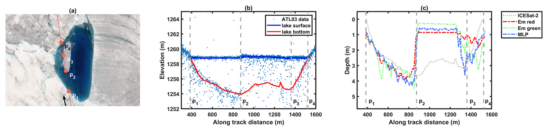
Figure 13 An example of the uncertainty in depth inversion in ice/snow-covered areas. (a) Sentinel-2 image obtained on 17 June overlaid with the ICESat-2 RGT 338. (b) The depth detection results by using kernel density estimation. (c) The depth inversion results by using the empirical formula and the MLP model.

5.2 The development characteristics of SGLs in the horizontal and vertical directions

By comparing the change characteristics of the SGL average area, depth, and volume over time, we find that there is a difference in the trend in lateral area development and vertical depth development throughout the development of SGLs from their incipient stages to their peak during the melt season (Fig. 14). From the initial melt period of 7 June to 2 July, the mean area and the mean depth develop together. However, from 2 to 14 July, the mean area continues to grow, while the mean depth decreases, implying that more new, shallow SGLs appear. This disparity is the causative factor for the observed trend of a decline in average depth before attaining its peak value. Before reaching the greatest mean depth, SGLs undergo lateral expansion in area, as evidenced by the fact that the rate of increase in mean area was faster than the growth in mean volume from 2 to 14 July. After this period, SGLs develop vertically in depth. From 14 July to 1 August, the mean volume continues to grow, reaching its maximum on 1 August. This result is similar to the findings of Pitcher and Smith (2019), who observed that supraglacial streams first incise, resulting in large changes in depth relative to width, and then ablation along channel walls results in lateral expansion, increasing width relative to depth. In addition to the variations in supraglacial lake development resulting from the topography of different regions, further investigation is required to better understand the rate of horizontal and vertical development during the ablation season.

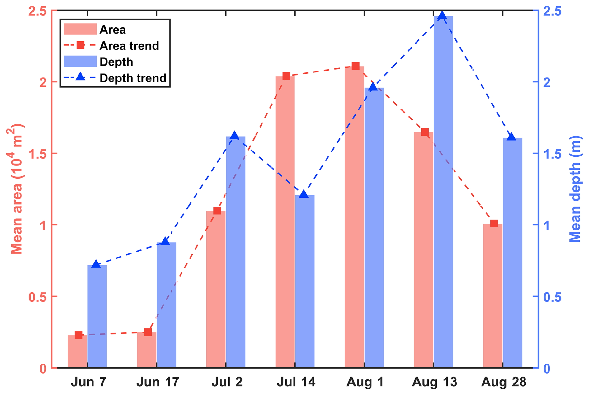
Figure 14 The trend in lateral area development and vertical depth development throughout the melt season.

6 Conclusions

A method for inverting the volume of SGLs by integrating optical imagery (Sentinel-2) and satellite altimetry data (ICESat-2) is proposed in this paper. It is indicated that the accuracy of SGL area extraction by using an RF model based on Sentinel-2 imagery is 90.20 %. And the mean absolute error of depth inversion by using an MLP model based on the ratio of reflectance oriented from Sentinel-2 imagery and the depth of SGLs detected by ICESat-2 data is 0.42 m, surpassing that of traditional empirical formula methods. The proposed volume inversion method for SGLs is applied to southwestern Greenland, thereby obtaining the volumetric evolution of SGLs throughout the entire melt season of 2022. It reveals that SGLs vary significantly in distribution, area, depth, and volume throughout the melt season. The SGLs evolve along coastlines and later spread inland, expanding in area and depth. The maximum total volume of SGLs is reached on 1 August, amounting to 9.30 × 10⁸ m³. Afterwards, SGLs above 1200 m continue to increase in volume, while SGLs below 1200 m begin to decrease. In late August, as the melt season draw to a close, SGLs diminish and retreat to coastal regions, with a notable reduction in volume. Moreover, the evolution characteristics of SGLs at different elevations are also investigated. It is found that the mean area, mean depth, and mean volume of SGLs below 800 m remain relatively stable throughout the entire melt season. SGLs above 800 m exhibit a similar evolution pattern, and the elevation range of 1200 to 1600 m is the most favorable for the evolution of SGLs. Moreover, our research indicates a temporal lag in the maximization of mean area and depth. At the onset of development, the area and depth evolve concurrently. Then, before the instance when the total volume of meltwater reaches its maximum (1 August), the mean area reaches its peak before the mean depth. This suggests that the SGLs exhibit velocities of morphological evolution along horizontal and vertical dimensions. The quantitative parameter inversion and analysis of SGLs in southwestern Greenland presented in this paper contribute to a better understanding of the mass balance of the Greenland ice sheet. However, when the surface of an SGL is covered with ice/snow, the depth may be underestimated, which could further lead to an underestimation of its volume. It may be possible to improve the accuracy of volume estimation by incorporating the temporal changes of the SGL over the time series.