Automatic grounding line delineation of DInSAR interferograms using deep learning

The regular and robust mapping of grounding lines is essential for various applications related to the mass balance of marine ice sheets and glaciers in Antarctica and Greenland. Differential Interferometric Synthetic Aperture Radar (DInSAR) enables precise detection of tide-induced ice shelf flexure at a continent-wide scale with temporal resolutions of just a few days. While automated pipelines for generating differential interferograms are well established, grounding line delineation remains largely a manual process, which is labor-intensive and increasingly impractical given the growing data streams from current and upcoming synthetic aperture radar (SAR) missions. To address this limitation, we developed an automated pipeline employing the holistically nested edge detection (HED) neural network to delineate grounding lines from DInSAR interferograms. The network was trained in a supervised manner using 421 manually annotated grounding lines of outlet glaciers and ice shelves of the Antarctic Ice Sheet. We also evaluated the utility of non-interferometric features such as surface elevation, ice velocity, and differential tide levels for enhancing delineation performance. Our recommended neural network, trained on the real and imaginary interferometric features, achieved a median offset of 265 m and a mean offset of 421 m from manual grounding line delineations, as well as a predictive uncertainty of 401 m. Furthermore, we demonstrated this network's capacity to generalize by generating grounding lines for previously undelineated interferograms, highlighting its potential for large-scale, high-resolution spatiotemporal mappings.

1 Introduction

Over the past 3 decades, there has been a clear negative trend in ice mass loss from both the Antarctic Ice Sheet (AIS) and the Greenland Ice Sheet (Otosaka et al., 2023; Fox-Kemper et al., 2021). However, projections of sea level rise from ice sheet evolution models remain highly uncertain, particularly for the AIS (Robel et al., 2019; Pattyn and Morlighem, 2020; Seroussi et al., 2020; Aschwanden et al., 2021). A primary source of this uncertainty is the limited understanding of dynamic processes at ice–ocean boundaries, further exacerbated by a scarcity of observations at the grounding line (Rignot, 2023). The grounding line (GL), where grounded ice transitions to floating ice shelves (Weertman, 1974), is a critical indicator of ice sheet stability and plays a key role in mass balance assessments (Rignot and Thomas, 2002; Rignot et al., 2008). Melting of ice shelves from contact with warm circumpolar deep water leads to GL retreat, making accurate and frequent mapping of GL position essential for monitoring ice sheet stability (Rignot and Jacobs, 2002; Depoorter et al., 2013; Schoof, 2007).

Detecting the precise location of the grounding line is challenging due to its subglacial location. This problem is addressed by considering other features as proxies for the true GL (Fig. 1a) (Brunt et al., 2011). Terrestrial and airborne ice-penetrating radar provide direct GL measurements (Jacobel et al., 1994; Catania et al., 2010; MacGregor et al., 2011; Uratsuka et al., 1996), while tiltmeter (Stephenson and Doake, 1979; Stephenson, 1984; Smith, 1991), static GPS (Riedel et al., 1999), and kinematic GPS (Vaughan, 1994) measurements capture the hinge line position F. Although spatial and temporal coverage is limited, these ground-based methods validate satellite-derived GLs.

Satellite remote sensing has significantly improved the spatial and temporal coverage of GL observations. Early satellite-based methods involved manual tracing of the break in slope I_b using Landsat 7 imagery (Bindschadler and Choi, 2011) and surface morphology derived from MODIS images (Scambos et al., 2007). Elevation profiles from radar altimetry (Dawson and Bamber, 2017, 2020; Hogg et al., 2018) and laser altimetry (Fricker and Padman, 2006; Fricker et al., 2009; Brunt et al., 2010, 2011; Li et al., 2020) have provided pointwise measurements of F, H, and I_b. F has also been inferred from radar line-of-sight displacement fields (Marsh et al., 2013; Christianson et al., 2016; Joughin et al., 2016) derived from differential range offset tracking (DROT). Recently, Wallis et al. (2024) correlated DROT range offsets with modeled tide levels to detect the transition between grounded and floating ice. These methods, alongside various static and dynamic approaches, have been comprehensively reviewed by Friedl et al. (2020).

Differential Interferometric Synthetic Aperture Radar (DInSAR) is regarded as the most accurate technique for GL detection (Rignot et al., 2011). A DInSAR interferogram is computed as the difference of two interferograms formed from three or more repeat-pass SAR acquisitions. If the assumption of constant ice velocity within the temporal baseline of the SAR acquisitions holds, the resulting differential interferogram contains detectable phase changes from the tidal flexure at the ice-sheet–ice-shelf boundary. The zone of ice shelf flexure is visible as a dense fringe belt in the DInSAR phase. The landward extent of the fringe belt is manually digitized as the grounding line. Figure 1b illustrates the flexure zone and digitized GL in the DInSAR interferogram of a glacier draining into the Ross Ice Shelf. The landward extent is typically within a few hundred meters seawards of F and considered a good approximation of the true grounding line (Rignot et al., 2011; Friedl et al., 2020). Two Antarctica-wide datasets have been generated with this method (Rignot et al., 2016; Groh, 2021a).

A less common approach is to unwrap the DInSAR phase and fit the resulting elevation data to a 1D elastic beam model, which relates the hinge line location to the vertical displacement of ice (Rignot, 1996). However, this technique is restricted to slow-moving glaciers, as phase decorrelation over fast-flowing ice streams limits the reliability of elevation estimates from phase unwrapping (Mouginot et al., 2019). Another approach derives tidal bending from individual interferograms and identifies the GL position through model inversion (Parizzi, 2020). This method avoids phase unwrapping and double-difference interferograms but requires an a priori estimate of the grounding zone location to constrain the phase gradient profiles, making it more semiautomatic.

Given the growing volume of SAR acquisitions suited to detect the grounding line from current (Sentinel-1 A, TerraSAR-X, COSMO-SkyMed, PAZ, ICEYE constellation) and upcoming missions (Sentinel-1 C, NISAR), replacing the labor-intensive manual grounding line delineation with scalable and automatic algorithms is necessary. Mohajerani et al. (2021) is the only study to date that applies deep learning for delineating the grounding line in double-difference interferograms. They used a convolutional neural network (CNN) based on the DeepLabV3+ architecture (Chen et al., 2018) and trained it on the real and imaginary components of 252 Sentinel-1 DInSAR interferograms of the Getz Ice Shelf. They delineated grounding lines for the rest of AIS on interferograms of 6 and 12 d repeat-pass Sentinel-1 acquisitions of 2018. They reported a mean deviation of 232 m between the network and manual digitizations and a median absolute deviation (MAD) of 101 m.

Building on our initial papers (Ramanath Tarekere, 2022; Ramanath Tarekere et al., 2023), this study advances automated GL detection by training a CNN to segment grounding lines directly from DInSAR phase data. In Ramanath Tarekere (2022), we conducted experiments to determine the optimal network and dataset parameters for this task, comparing the performance of holistically nested edge detection (HED) (Xie and Tu, 2015) and UNet (Ronneberger et al., 2015) architectures for GL delineation. Several tile dimensions and resolutions were tested to derive the best dataset configuration. Ramanath Tarekere et al. (2023) fine-tuned the HED network from Ramanath Tarekere (2022); introduced minor network adjustments; and explored the influence of topographical, meteorological, and ice flow data on GL delineation. In this work, we expand on the topic of feature importance, determine an effective dataset split strategy for training the network, and demonstrate the network's spatial transference ability by delineating interferograms from regions previously unseen during network training. Additionally, we provide predictive model uncertainties.

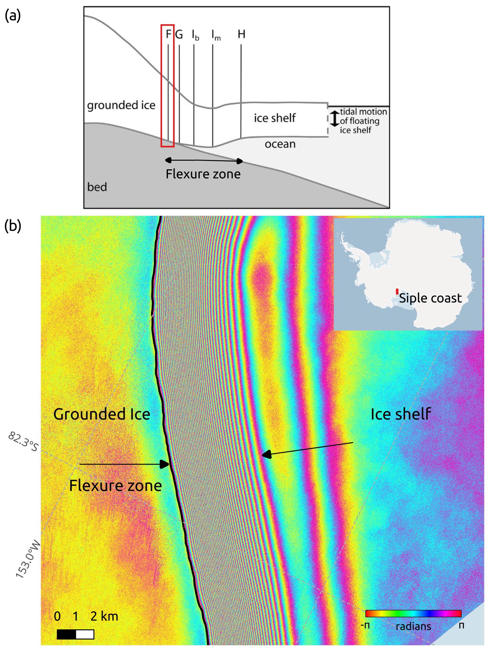
Figure 1 (a) The cross-section of an ice shelf, showing the features in the flexure zone: F (hinge line) is the landward limit of the ice flexure due to tides, G is the true grounding line, I_b is the break in slope, I_m is the local elevation minimum, and H is the seaward limit of ice flexure where the ice shelf reaches hydrostatic equilibrium. Adapted from Fricker et al. (2009). (b) DInSAR interferogram from four TerraSAR-X acquisitions of an outlet glacier located in the Siple coast with 11 d temporal baseline. The black line shows the manually delineated GL (point F in a). The black arrows at the edges of the dense fringe belt show the extent of the flexure zone in the interferogram.

2 Dataset

2.1 The AIS_cci grounding line location

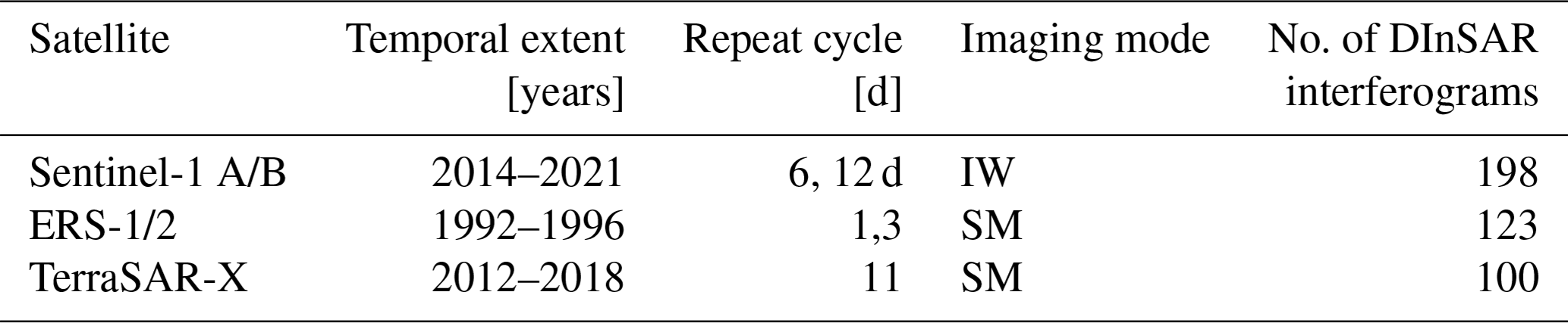
We used manual GL delineations from the grounding line location (GLL) product of ESA’s Antarctic Ice Sheet Climate Change Initiative project (hereafter AIS_cci GLL) as labels for training the neural network and to validate its performance. The interferometric processing was carried out with a pipeline developed at the Remote Sensing Technology Institute in the German Aerospace Center (DLR), within the AIS_cci project (Muir, 2020). The GL digitizations are available as “LineStrings” in an Esri shapefile, including metadata about acquisition conditions, tide levels, and atmospheric pressure. A complete product description can be found in Groh (2021a). For this study, we used the manual delineations of 421 interferograms formed from Sentinel-1, ERS-1/2 and TerraSAR-X acquisitions. Table 1 provides details regarding the temporal coverage, temporal baselines, and the number of double-difference interferograms generated from the acquisitions of the missions mentioned above. Only a subset of the original dataset is openly accessible (Floricioiu et al., 2021). The map in Fig. 2a shows the spatial extent of the AIS_cci GLLs.

Table 1 Overview of the satellite acquisitions of the interferograms used in the AIS_cci GLL product. IW: interferometric wide swath; SM: strip map. The last column shows the number of double-difference interferograms used in this study.

2.2 Training features stack

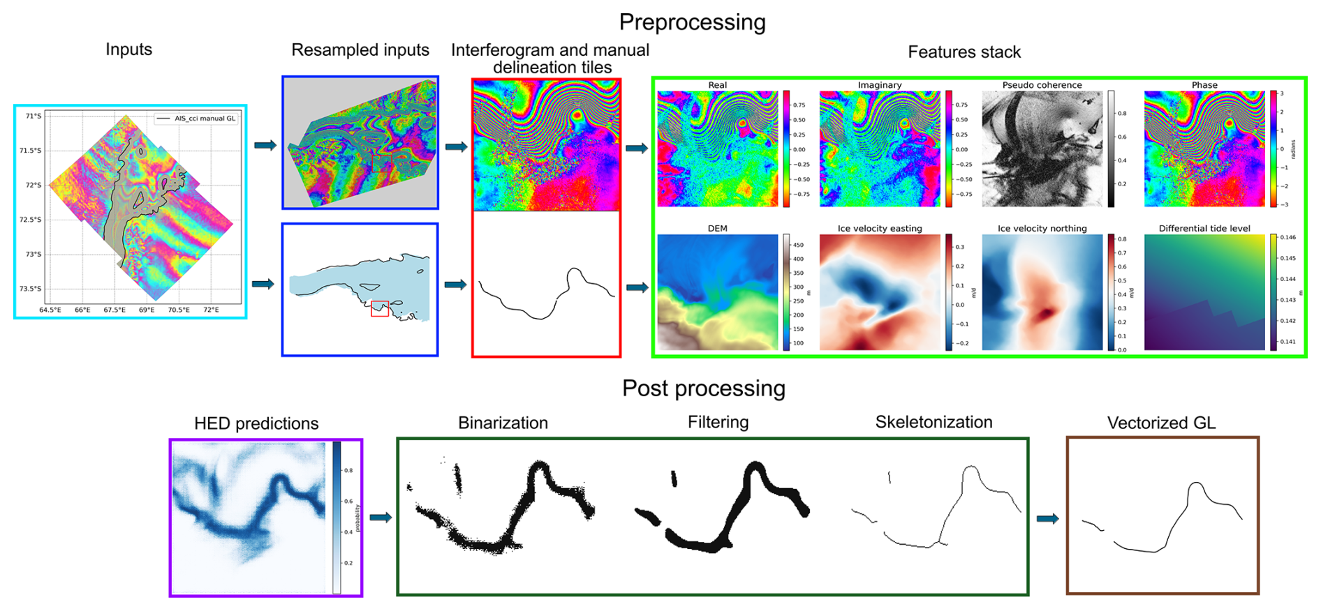
To train our neural network, we compiled a stack of eight interferometric and non-interferometric features derived from various datasets. Table 2 summarizes these feature attributes, and Fig. 2b and c present examples of the complete feature set for one sample.

2.2.1 Interferometric features

The interferometric features were generated from the double-difference wrapped phases used in the AIS_cci GLL production pipeline. These features include the real and imaginary components of the double-difference interferograms, the wrapped phase, and pseudo-coherence (Fig. 2b). Pseudo-coherence arises from resampling the wrapped phase images while preserving the cyclic phase variations from −π to π. Additional details on this process are provided in Appendix A. Pseudo-coherence reflects phase stability, with higher values in areas of lower fringe frequency. However, it is not an objective measure of phase quality. Both decorrelated pixels and pixels with high fringe frequency but good coherence exhibit low pseudo-coherence values (below 0.4).

2.2.2 TanDEM-X PolarDEM

Surface elevation data were sourced from the 90 m resolution TanDEM-X PolarDEM of Antarctica (Huber, 2020), derived from the global TanDEM-X digital elevation model (Wessel, 2016). The TanDEM-X PolarDEM was created by averaging two complete coverage datasets from bistatic acquisitions between April 2013 and November 2013 and between April 2014 and October 2014. Additional acquisitions from July 2016 to September 2017 were used to fill gaps. Further information on the generation, calibration, and validation of TanDEM-X PolarDEM can be found in Wessel et al. (2021).

2.2.3 Ice velocity from Sentinel-1

Ice velocity data were produced by the consortium partner ENVEO IT as part of the AIS_cci project (Wuite, 2020) (available at http://cryoportal.enveo.at, last access: 3 July 2025). This 3D product includes easting, northing, and vertical velocity components. Azimuth and line-of-sight (LOS) velocities, derived from Sentinel-1 SAR backscatter image offset tracking (Nagler et al., 2015), were projected onto the Reference Elevation Model of Antarctica (REMA) digital elevation model (Howat et al., 2019). The resulting velocity map represents a multiyear average from Sentinel-1 repeat-pass data acquired between 2014 and 2021, covering the continental margins up to approximately 75° S. In our feature stack, we included only the northing and easting components, as horizontal ice flow may help the neural network distinguish between grounded and floating ice on a coarse spatial scale.

2.2.4 Ocean tide levels from the Circum-Antarctic Tidal Simulation (CATS2008)

The differential tidal state captured in the DInSAR data was computed by combining individual tide levels from the CATS2008 tide model (Padman et al., 2008) in the same sequence as the interferograms used to create the double difference. The CATS2008 model incorporates data from tide gauges, GPS measurements, TOPEX/Poseidon radar altimetry, ICESat-derived grounding line locations, and Mosaic of Antarctica (MOA) grounding lines. Although the model is gridded at 4 km, we obtained pixel-wise interpolated tide levels using the pyTMD module (Sutterly et al., 2017) in Python. We further corrected the tide levels for the inverse barometer effect (Padman et al., 2003) by incorporating daily air pressure data from the National Centers for Environmental Prediction and the National Center for Atmospheric Research Reanalysis (NCEP/NCAR), provided by NOAA PSL, Boulder, Colorado, USA (https://psl.noaa.gov, last access: 3 July 2025). The final corrected tidal amplitudes were included in the training feature stack.

(Groh, 2021a)(Groh, 2021b)(Huber, 2020)(Wessel et al., 2021)(Wuite, 2020)(Nagler et al., 2015)(Padman et al., 2008)(McMillan et al., 2011)

Table 2 Attributes of the input features used to train the neural network. No temporal coverage is specified for CATS2008 because the model assimilates several measurements across various time periods and provides the tidal amplitude for the required epoch. The mentioned pixel sizes of the double-difference interferograms are after geocoding and are therefore square.

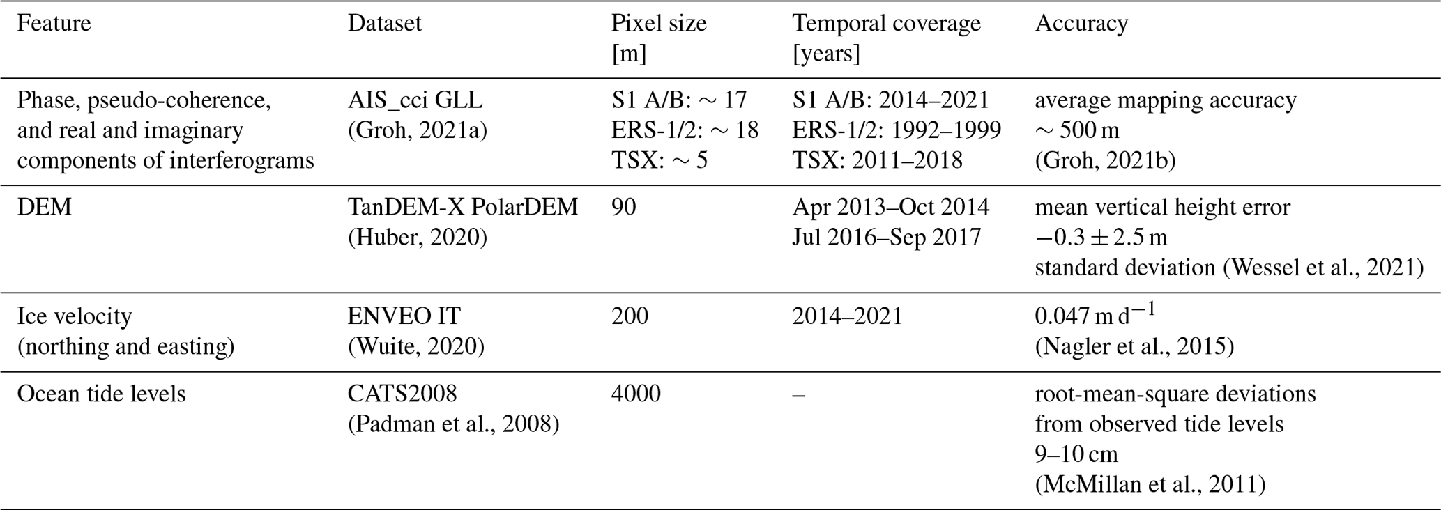
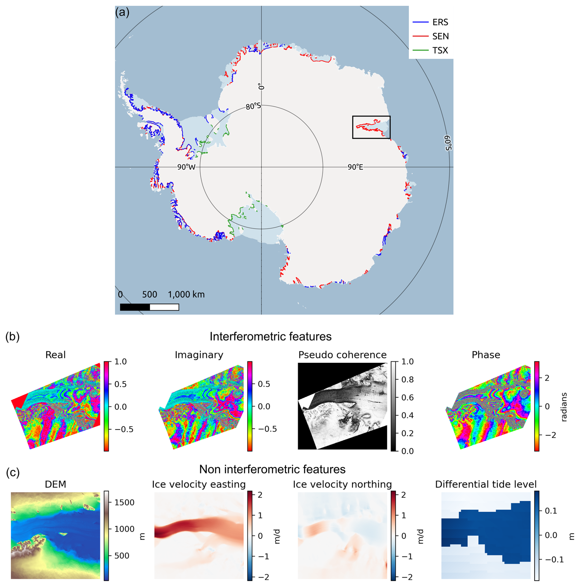
Figure 2 (a) Manual grounding line delineations from the AIS_cci GLL dataset (Groh, 2021a). The legend shows the satellite missions used to derive the DInSAR interferograms: ERS – European Remote Sensing Satellite; SEN – Sentinel-1 A/B; TSX – TerraSAR-X. The rectangles below the map show (b) interferometric features and (c) non-interferometric features for the Amery Ice Shelf (black rectangle in a).

3 Automatic delineation pipeline

3.1 Preprocessing

Each component of the feature stack requires preprocessing before being input into the neural network. The AIS_cci GLL line geometries are converted into rasters with a pixel size of 100 m. The double-difference interferograms are resampled to match this raster grid. The GL and interferogram rasters are then tiled into 256×256 pixel patches with 20 % overlap in all directions. The feature stack described in Sect. 2.2 is cropped accordingly to form a three-dimensional array. Missing pixels are filled with the mean value of the corresponding feature within the tile. Non-interferometric features are normalized to the range 0 to 1 to ensure network stability during training. The tiles are split into training, validation, and test sets. To augment the training data, random horizontal and vertical flips are applied, doubling the number of samples. These preprocessing steps are illustrated in Fig. 3.

3.2 GL delineation

We trained a holistically nested edge detection (HED) network (Xie and Tu, 2015) to delineate GLs. Our architecture closely follows the original design, with modifications to the padding scheme to maintain spatial dimensions across convolutions. The network consists of five convolutional blocks, each containing 3×3 convolutions, with max pooling layers downsampling the output by a factor of 2 between blocks (Fig. B1). The final segmentation map is a weighted combination of outputs from all blocks, upsampled to a uniform size before concatenation. To address the class imbalance between GL and background pixels, we applied the weighted cross-entropy loss proposed by Xie and Tu (2015):

$$\begin{array}{}\text{(1)}& L\left(\widehat{y}\right)=-{\displaystyle \frac{\left|y_{\mathrm{gl}}\right|}{\left|y\right|}}\sum _{j\in y_{\mathrm{bg}}}\log (\mathrm{1}-\widehat{y_j})-{\displaystyle \frac{\left|y_{\mathrm{bg}}\right|}{\left|y\right|}}\sum _{j\in y_{\mathrm{gl}}}\log \widehat{y_j},\end{array}$$

where $\left|y_{\mathrm{gl}}\right|$ is the number of grounding line pixels, $\left|y_{\mathrm{bg}}\right|$ is the number of background pixels, and $\left|y\right|$ is the total number of pixels for one sample. The function weights the predicted probabilities of grounding line pixels by the fraction of background pixels and vice versa for each tile.

We apply this loss function to each side output to enhance the learned features in the network's initial layers. This technique, called deep supervision, has been demonstrated to improve generalization and mitigate the challenge of vanishing gradients in segmentation tasks (Lee et al., 2015; Xie and Tu, 2015). Furthermore, the Rectified Linear Unit (ReLU) activation function is employed for every convolution layer, while the sigmoid function is applied to both the side outputs and the concatenated output. Once the neural network has been trained with the specified parameters outlined in Sect. 3.4, we input the test samples into the network. This generates segmentation maps where each pixel denoted the probability of belonging to the grounding line class.

Figure 3 Flowchart outlining the operations in our automatic delineation pipeline. The colored borders of each step correspond to the illustrations depicted in Fig. 4.

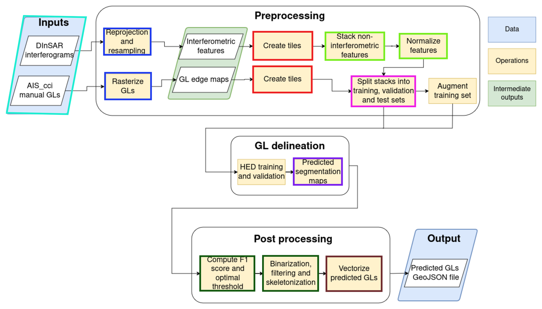
3.3 Postprocessing

Following the delineation module, postprocessing is applied to refine the output segmentation maps by removing uncertain or spurious predictions. This filtering procedure comprises three stages. First, the segmentation maps are converted into binary images by applying a fixed threshold. Pixels with values greater than or equal to the threshold are assigned a value of 1, while the remaining pixels are set to 0. Next, a median filter with a window size of 3 is applied to the binarized predictions to eliminate noise and small spurious branches. Subsequently, a skeletonization algorithm (Zhang and Suen, 1984) is employed to iteratively thin the prediction rasters until only a one-pixel-wide skeleton remains. To further refine the results, the skeletonized predictions are pruned to remove small side branches using the PlantCV Python library (Gehan et al., 2017). Finally, the cleaned skeletons are converted into line vectors and saved as GeoJSON files for downstream analysis. The schematic representation of this delineation pipeline is illustrated in Fig. 3. An example output for an interferogram, along with its manual delineation, is provided in Fig. 4.

Figure 4 Illustration of the steps described in the delineation pipeline flowchart (Fig. 3) for an exemplary interferogram of the Amery Ice Shelf (black rectangle in Fig. 2). The colors of the outlines of each image correspond to the respective highlighted operation in Fig. 3.

3.4 Training scheme

We trained our models on the NVIDIA A100 GPU with 80 GB high-bandwidth memory for a maximum of 100 epochs and a batch size of 128 tiles. We used the Adam optimizer with parameters recommended by Kingma and Ba (2017) and a learning rate of $\mathrm{3}\times {\mathrm{10}}^{-\mathrm{4}}$. The neural network was implemented in the PyTorch Lightning framework (Falcon and The PyTorch Lightning team, 2019).

To simulate real-world conditions, we employed two distinct data-splitting approaches: spatial and temporal variants. In the temporal split (Fig. 5a), samples are drawn from the same regions of interest (ROIs) but split based on acquisition time, with the training set containing multiple time points and validation and test sets representing different time periods within the same regions (Fig. 5c, d, g). This approach better reflects operational settings where future observations typically originate from previously observed areas. In the spatial split (Fig. 5b), training, validation, and test samples are drawn from completely different geographic regions, ensuring that the model is evaluated on unseen locations (Fig. 5e, f, i, j). This approach prevents the model from relying on regional similarities present in the training data. However, in data-scarce ROIs – such as glaciers with limited temporal coverage – all samples may end up in the training set due to the lack of sufficient observations for validation and testing. This fallback scenario closely resembles the spatial split and is illustrated in Fig. 5h and j, which are identical to emphasize that some regions only contribute to the training set in the temporal split. The temporal split comprises 4227 training samples, 121 validation samples, and 308 test samples. The spatial split consists of 4223 training samples, 118 validation samples, and 589 test samples.

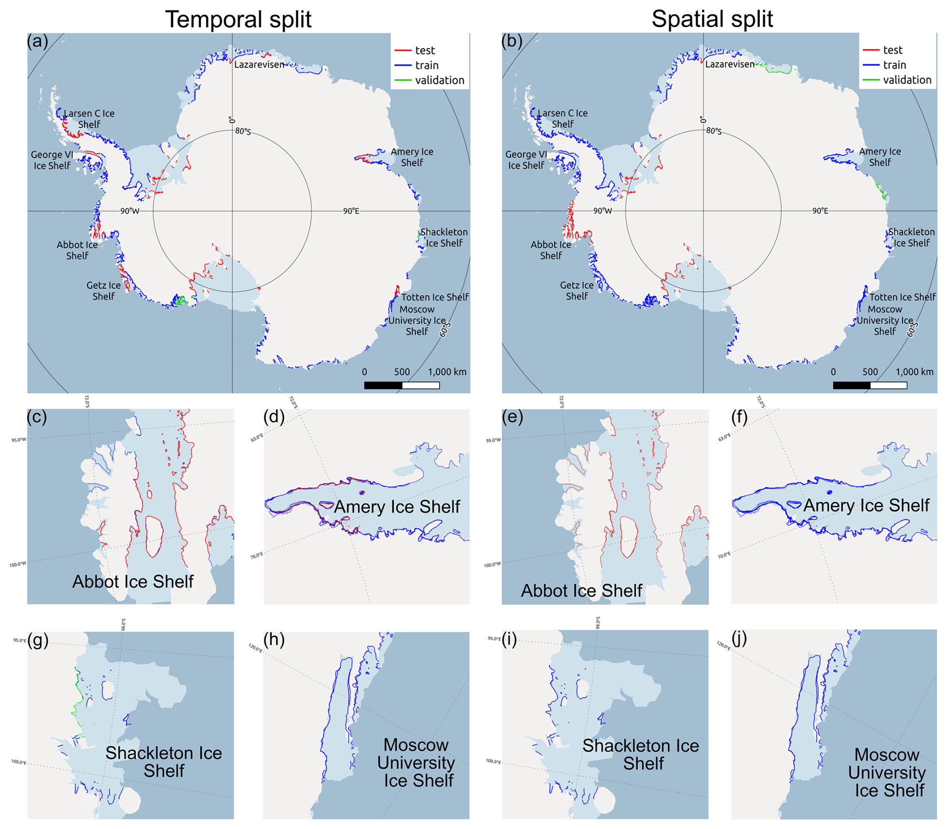
Figure 5 Distribution of the AIS_cci lines into training (blue), validation (green), and test (red) sets of (a) temporal and (b) spatial splits. The temporal samples for (c) Abbot Ice Shelf and (d) Amery Ice Shelf contain spatially overlapping but temporally separated training and test samples. In contrast, the spatial samples for the same regions contains only (e) test samples or (f) training samples. The temporal data for the (g) Shackleton Ice Shelf contains training and validation samples, whereas the (h) Moscow University Ice Shelf samples contain only training samples. The spatial data for (i) Shackleton Ice Shelf and (j) Moscow University Ice Shelves contain only training samples.

3.5 Performance evaluation metrics

The evaluation of the segmentation performance and delineation quality was carried out using both pixel-wise and geometry-based metrics.

Pixel-wise segmentation performance was assessed using the optimal dataset F₁ score (ODS F₁) and average precision (AP). The F₁ score (Eq. 2) is the harmonic mean of precision (P) and recall (R). ODS F₁ is computed by converting predictions into binary maps at the threshold yielding the highest F₁ score across all samples; for our dataset, this threshold is 0.8. AP (Eq. 3) is calculated as the weighted average of precision values across all thresholds, considering the increase in recall.

$$\begin{array}{}\text{(2)}& F_{\mathrm{1}}=\mathrm{2}\times {\displaystyle \frac{P\times R}{P+R}}\text{ with }P={\displaystyle \frac{T_{\mathrm{p}}}{T_{\mathrm{p}}+F_{\mathrm{p}}}}\text{ and }R={\displaystyle \frac{T_{\mathrm{p}}}{T_{\mathrm{p}}+F_{\mathrm{n}}}},\end{array}$$

where T_p represents true-positive, F_p represents false-positive, and F_n represents false-negative pixels.

$$\begin{array}{}\text{(3)}& \text{AP}=\sum _n(R_n-R_{n-\mathrm{1}})\times P_n,\end{array}$$

where P_n and R_n are the precision and recall at the nth threshold.

To evaluate the positioning accuracy of postprocessed GL delineations, we used the polygons and line segments (PoLiS) metric (Avbelj et al., 2014). PoLiS measures the average distance between the vertices of two line geometries. Given that our delineations are line geometries, we calculated the Euclidean distance from each point on the network-generated GL to its closest point on the corresponding manual GL (Eq. 4). This is closely related to the mean distance error (MDE) (Gourmelon et al., 2022), but PoLiS is designed specifically for vector geometries.

$$\begin{array}{}\text{(4)}& p(A,B)={\displaystyle \frac{\mathrm{1}}{\mathrm{2}\left|A\right|}}\sum _{a\in A}\underset{b\in B}{min}\Vert a-b{\Vert }_{\mathrm{2}}+{\displaystyle \frac{\mathrm{1}}{\mathrm{2}\left|B\right|}}\sum _{b\in B}\underset{a\in A}{min}\Vert b-a{\Vert }_{\mathrm{2}},\end{array}$$

where $\left|A\right|$ refers to the total number of grounding line points in the manual delineation, and $\left|B\right|$ is the total number of grounding line points in the network-generated GL.

We also computed the fraction of the length of manual GLs identified by the neural network as the coverage percentage (Eq. 5). Only GL segments within the median PoLiS distance from the manual delineation are considered to exclude spurious predictions.

$$\begin{array}{}\text{(5)}& \text{Coverage}={\displaystyle \frac{\text{length of network-generated GL}}{\text{length of corresponding manual GL}}}\cdot \mathrm{100}\mathit{\%}\end{array}$$

4 Results and discussion

4.1 Importance of interferometric features

To evaluate the optimal representation of interferometric features, we trained two networks with different input representations: one using rectangular interferometric features and the other using polar interferometric features in their training feature stacks (denoted as network 1 and network 2 in Table 3, respectively). We used the training samples of the temporal dataset variant (Sect. 3.4, Fig. 5a) and evaluated the respective test set.

Both networks produced GLs with median distances of less than 300 m from manually delineated GLs. Visual assessments (Fig. 6) reveal that both networks are capable of tracing the complex GL geometry and distinguishing between the landward and seaward extents of the flexure zone. However, both networks struggle with accurately capturing sharply curving segments of the GL, leading to non-continuous delineations (Fig. 6a, b, c) and producing spurious branches (Fig. 6e, f). Although the visual agreement with manual delineations is promising, the segmentation metrics seem to indicate poor performance. Specifically, the average precision and ODS F₁ scores remain low due to high class imbalance between GL and background pixels. Predictions even one pixel away from the manual delineations are counted as false positives, leading to reduced precision and lower ODS F₁ scores. This is consistent with the findings of Heidler et al. (2022a) and Gourmelon et al. (2022). Given that final GLs are obtained only after postprocessing the output segmentation maps, the PoLiS distances provide a more accurate measure of delineation quality.

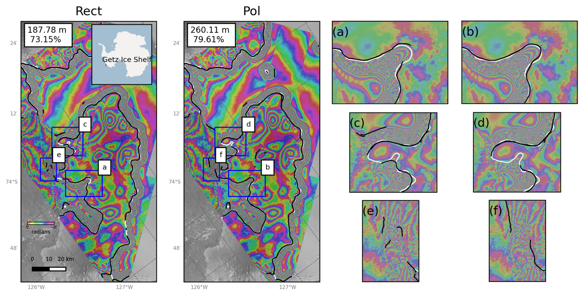
Figure 6 Comparison of manual (white) and network-generated (black) GLs overlaid on an interferogram of the Getz Ice Shelf, with the black lines representing outputs from networks 1 and 2 (see Table 3). The text boxes in the upper left of each panel show the average PoLiS distance between the manual and network-generated GLs, along with the fraction of the manual GL delineated. The right-side panels provide zoomed-in views of selected areas (marked by blue rectangles) to highlight specific cases: (a), (b), (c), and (d) show loose interferometric fringes not captured by the networks; (e) and (f) highlight spurious detections.

The observed disparity between mean and median PoLiS distances is driven by a subset of interferograms with low coherence, which results in sparse delineations. This also skews coverage percentages, leading to lower average coverage. Upon examining the phase images of these challenging samples (Fig. 7a, b, and the pinning point in c and d), it is clear that decorrelation adversely affects the delineation. These manual delineations highlight the variability in GL delineation by human operators. Notably, Mohajerani et al. (2021) found that neural network failures are generally more consistent than human inconsistencies.

Training the network with both rectangular and polar components did not yield improvements in performance (network 1 in Table C1). Since these features represent different formulations of the same underlying interferogram, we surmise that the network does not benefit from the redundancy. Notably, the network trained with rectangular features performed slightly better – both quantitatively and qualitatively – than the network trained with polar features. Therefore, we chose to proceed with rectangular features combined with various subsets of non-interferometric features for subsequent experiments.

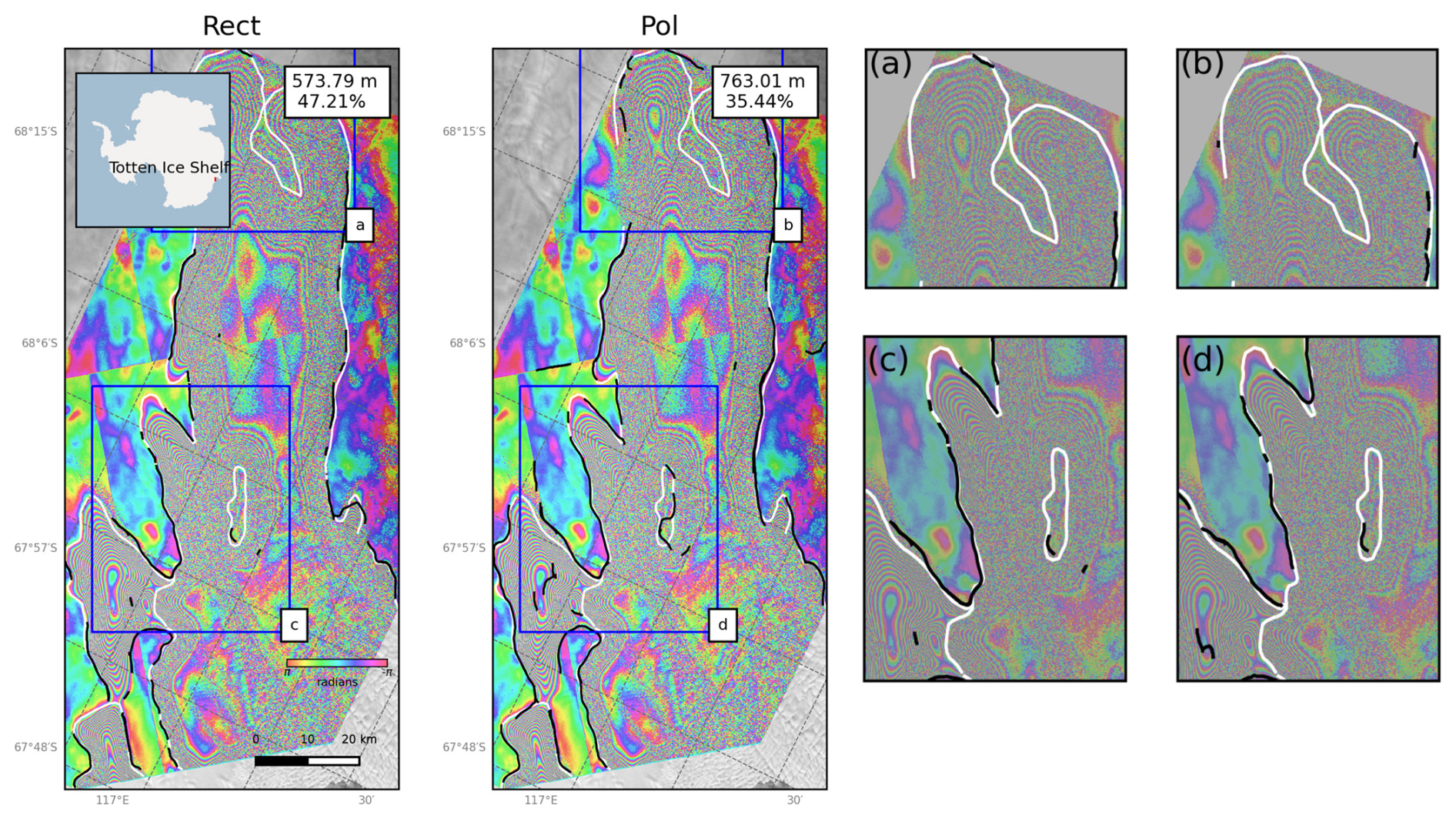
Figure 7 Visualization of the manual (white) and network-generated (black) GLs of the Totten Ice Shelf from networks 1 and 2 (Table 3). The zoomed-in panels (a), (b), (c), and (d) show decorrelated parts of the fringe belt which were not delineated by either network.

4.2 Importance of non-interferometric features

To assess the importance of non-interferometric features in GL delineation, we trained several networks using different combinations of rectangular interferometric features and non-interferometric features. These non-interferometric features (Fig. 2c) were evaluated using the leave-one-covariate-out (LOCO) inference method (Lei et al., 2018), which involves training models with specific feature subsets and comparing performance when each feature is individually removed. We trained the models using samples from the temporal dataset variant (Sect. 3.4, Fig. 5a) and evaluated their performance on the corresponding test set. The results are summarized in Table 3.

4.2.1 Influence of DEM

The addition of the DEM consistently improved network performance across multiple configurations (networks 4, 7, and 9). Network 4 (Rect + DEM) achieved a median PoLiS distance of 236.5 m and a mean coverage of 73.8 %, outperforming network 1 (Rect). The performance boost was even more evident in network 9 (Rect + DEM + Vel), which attained a median distance of 227.1 m and coverage of 74.7 %. We attribute this performance boost to the visibility of I_b, which aids in distinguishing the GL, particularly in regions where interferograms suffer from low coherence.

Table 3 Numerical results for networks trained with different feature subsets as described in Sect. 4.2. Abbreviations for feature subsets are as follows: Rect – real and imaginary components (rectangular representation); Pol – phase and pseudo-coherence (polar representation); DEM – digital elevation model; Vel – ice velocity (northing and easting components); Tide – differential tide level; Non-Intf – non-interferometric features. The best-performing network variant is highlighted in bold.

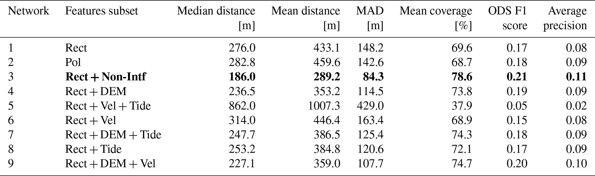
Table 4 Numerical results for the experiments described in Sect. 4.3. The networks were trained on the rectangular features of the respective datasets. The best-performing network variant is highlighted in bold.

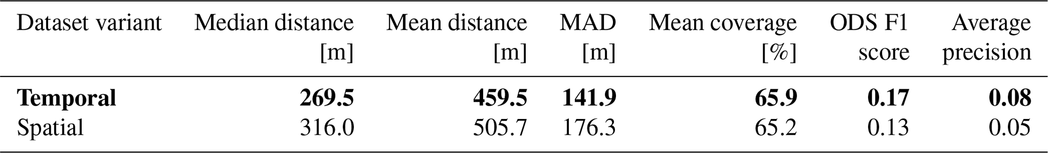
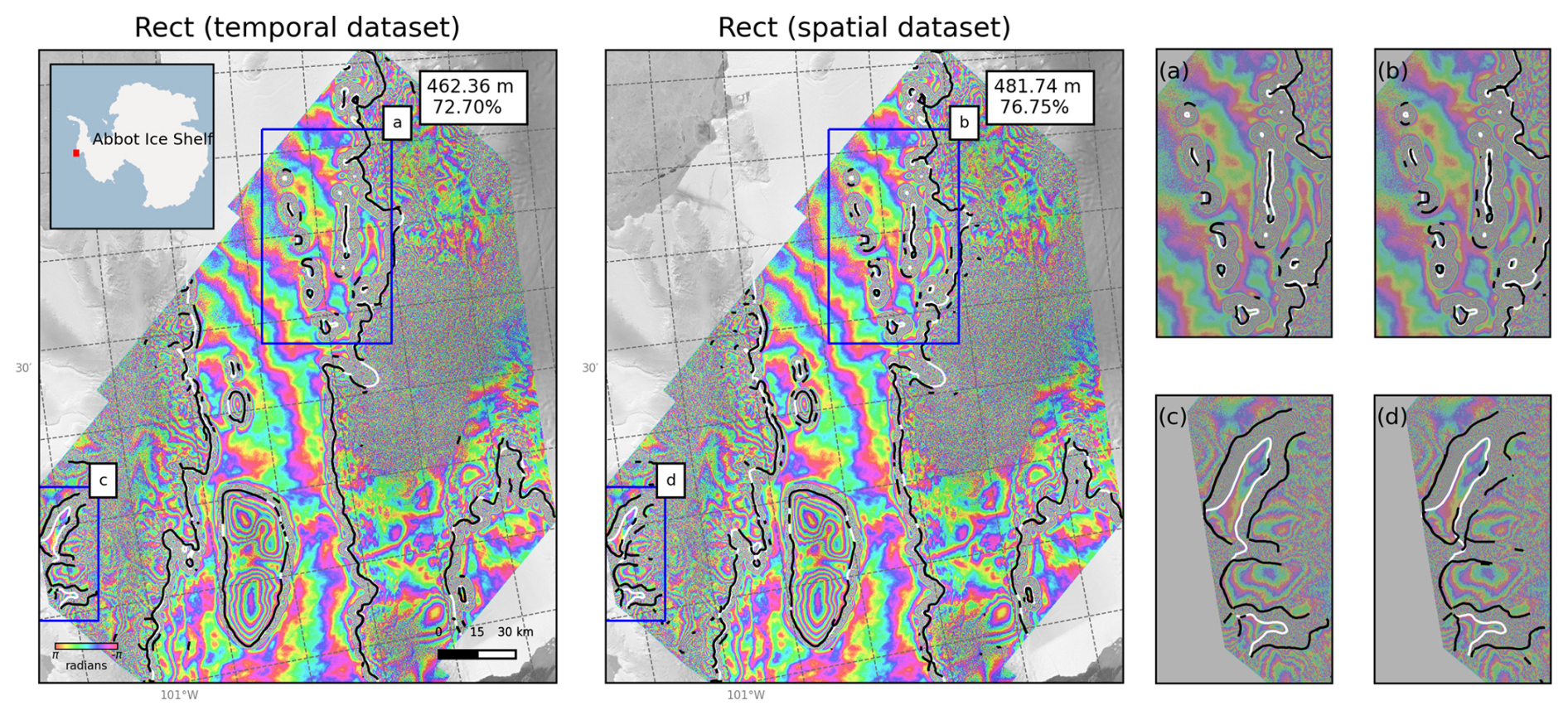
Figure 8 Delineations made by the HED (black) trained on the temporal dataset and spatial dataset for the Abbot Ice Shelf sample (Table 4). The close-ups in (a) and (b) show fragmented pinning point delineations made by the networks; (c) and (d) show the correct landward-fringe delineation. The manual delineation (white) is incorrectly made on the seaward-most fringe.

However, this benefit comes with potential drawbacks. The DEM is a mosaic derived from several years of SAR acquisitions (Sect. 2.2.2), meaning the break-in-slope feature may not precisely align with the GL captured in the DInSAR phase. Furthermore, the break-in slope is an unreliable proxy for fast-flowing glaciers. This introduces the risk that the network could overfit the DEM, producing inaccurate delineations – especially for fast-flowing glaciers, where interferometric coherence is often poor. While our evaluation found no strong evidence of this issue beyond a few isolated cases, similar overfitting has been observed in automatic calving front delineation models (Heidler et al., 2022b; Loebel et al., 2022). Although GL migration is generally slower than calving front dynamics, we caution users to ensure the region of interest is relatively stable when incorporating the DEM.

4.2.2 Influence of ice velocity and differential tides

In contrast, including ice velocity and differential tide features led to mixed results. Network 5 (Rect + Vel + Tide) performed the worst among all configurations, with a median distance of 862.0 m and a mean coverage of only 37.9 %. This performance gap suggests that these features alone provide insufficient information for accurate GL delineation. However, combining the differential tide individually with rectangular features (network 8) yielded moderate improvements over the network 1. Network 6 (Rect + Vel) performed marginally worse than network 1. Examples of delineations from these networks are shown in Fig. C3 (network 5) and Fig. C2 (networks 6 and 8).

4.2.3 Best-performing feature combination and operational recommendations

Network 3 (Rect + Non-Intf) achieved the best overall performance, with a median distance of 186.0 m and coverage of 78.6 %. However, our results indicate that the DEM is the primary driver of this performance gain, while the contributions of ice velocity and tide features remain unclear. The LOCO framework does not allow us to quantify their individual effects precisely. Despite network 3's superior performance, we recommend network 1 (Rect) for operational use for several practical reasons:

1. Using only interferometric features significantly reduces preprocessing time and storage requirements.

2. Although the DEM boosts performance overall, its potential to introduce errors in fast-flowing glaciers necessitates caution.

3. The interferogram is the only time-varying input, making it the most reliable indicator of the GL within the temporal context of the SAR acquisitions.

4.3 Inference on the spatial dataset variant and undelineated interferograms

To evaluate the generalization capabilities of HED, we applied the network trained on rectangular features from the temporal dataset variant (network 1 in Table 3) to delineate test samples from the spatial dataset variant. We compared these delineations to those produced by HED, trained specifically on the training samples from the spatial dataset. This experiment simulates an operational scenario in which the network is used to generate long-term time series of grounding lines (GLs) for glaciers and ice streams across Antarctica.

The quantitative evaluation showed that the temporal-trained network outperformed the spatial-trained network across all metrics (Table 4). The better performance of the temporal-trained network is likely due to its exposure to multiple interferograms from the same region during training, allowing it to generalize better. This suggests that the temporal-trained network is particularly well suited for generating time series of grounding lines in regions with a sufficient number of coherent interferograms. Despite these performance differences, the spatial-trained network nevertheless produced delineations over the Abbot Ice Shelf region that visually resembled those from the temporal-trained network, even though no training samples from this area were included in the spatial dataset (Fig. 5e). This suggests that the spatial-trained network has some capacity to generalize to previously unseen regions. Both networks struggled to identify and accurately delineate pinning points (Fig. 8a, b) but consistently delineated the landward side of the fringe belt, despite having been trained on isolated samples of inaccurate manual delineations positioned on the seaward side (Fig. 8c, d).

We further tested the spatial transferability of the temporal-trained network on previously unseen interferograms covering several glaciers draining into the Ross Ice Shelf, illustrated as black lines in Fig. 9a. These interferograms had not been manually delineated and were not part of the AIS_cci grounding line product. Despite having never seen these interferograms during training or validation, the network successfully delineated the landward-most fringe and avoided decorrelated fringes over the Crary Ice Rise and Nimrod Glacier (Fig. 9b, c). Similarly, the network avoided delineating the loose fringes in interferograms of Dickey Glacier and Nursery Glacier (Fig. 9d). In this context, the network complemented existing manual delineations by reducing gaps and producing a more complete grounding line for the region.

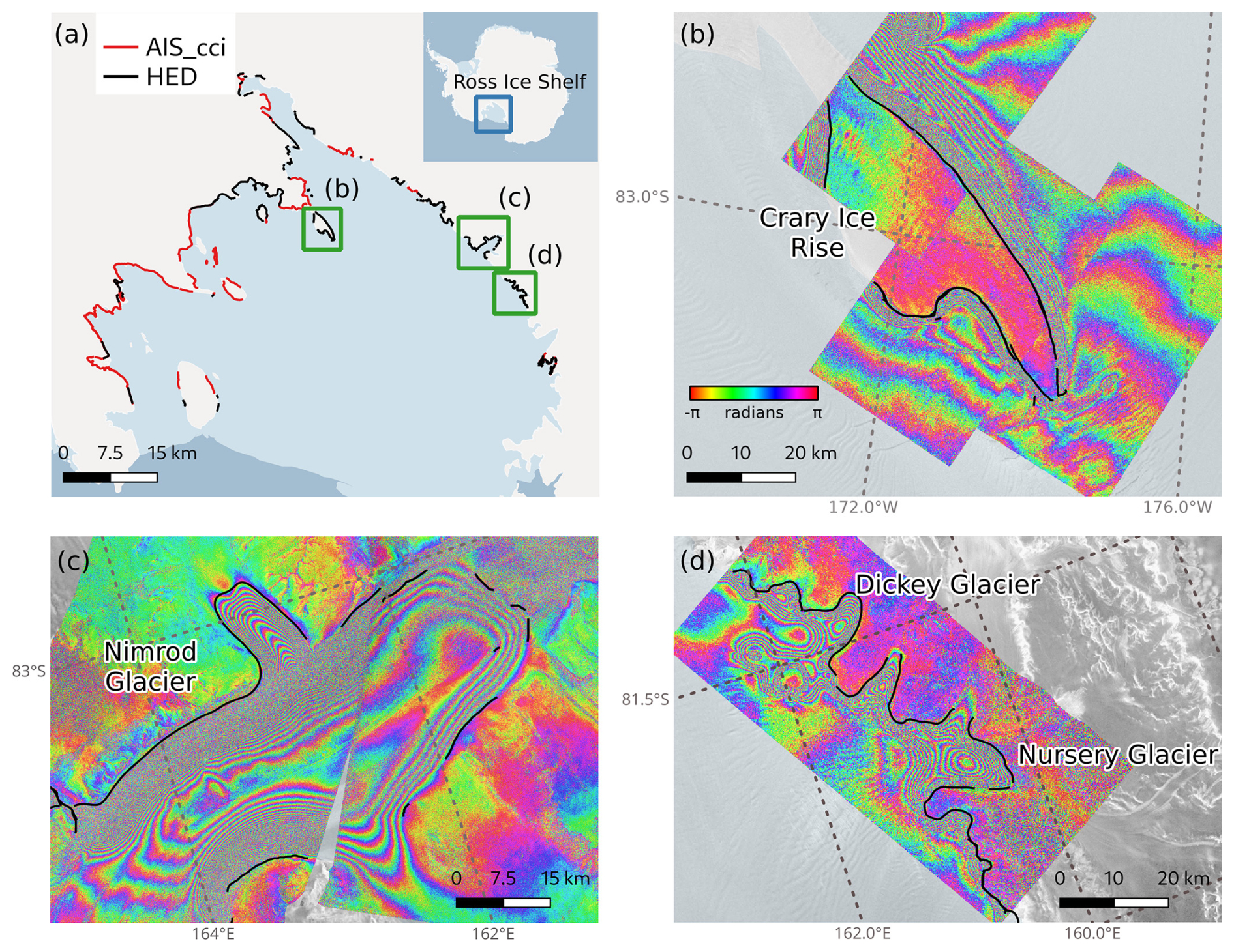
Figure 9 (a) AIS_cci GLL (red) and HED trained on the temporal dataset (black) grounding lines for several glaciers situated around the Ross Ice Shelf (upper left). HED delineations for interferograms over (b) Crary Ice Rise, (c) Nimrod Glacier, and (d) Dickey and Nursery glaciers. The discontinuous GLs for the Nimrod Glacier and Crary Ice Rise are from two spatially overlapping but temporally separate DInSAR interferograms. The interferograms appear brighter in the overlapping regions.

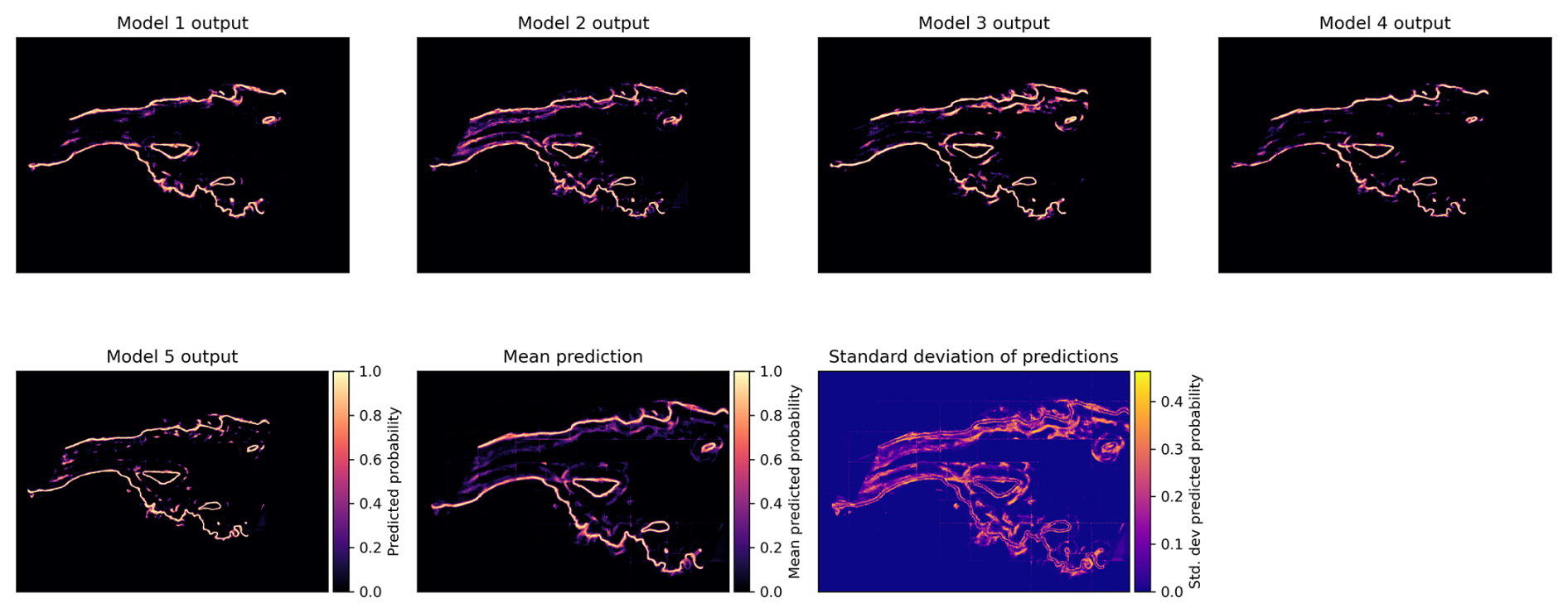
Figure 10 Example of mean and standard deviation of an ensemble of five predictions computed for a test sample of the Amery Ice shelf. The networks were trained with rectangular features. Models 1–5 share the color bar which is displayed to the right of the model 5 output.

Table 5 Performance of ensemble networks described in Sect. 5. The metrics are calculated for the ensemble average GLs. The predictive error is computed as the average of one-way distances from the average GLs to the nearest uncertainty buffer contour. Abbreviations for feature subsets are as follows: Rect – real and imaginary components (rectangular representation); Non-Intf – non-interferometric features.

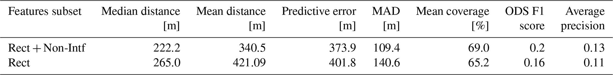
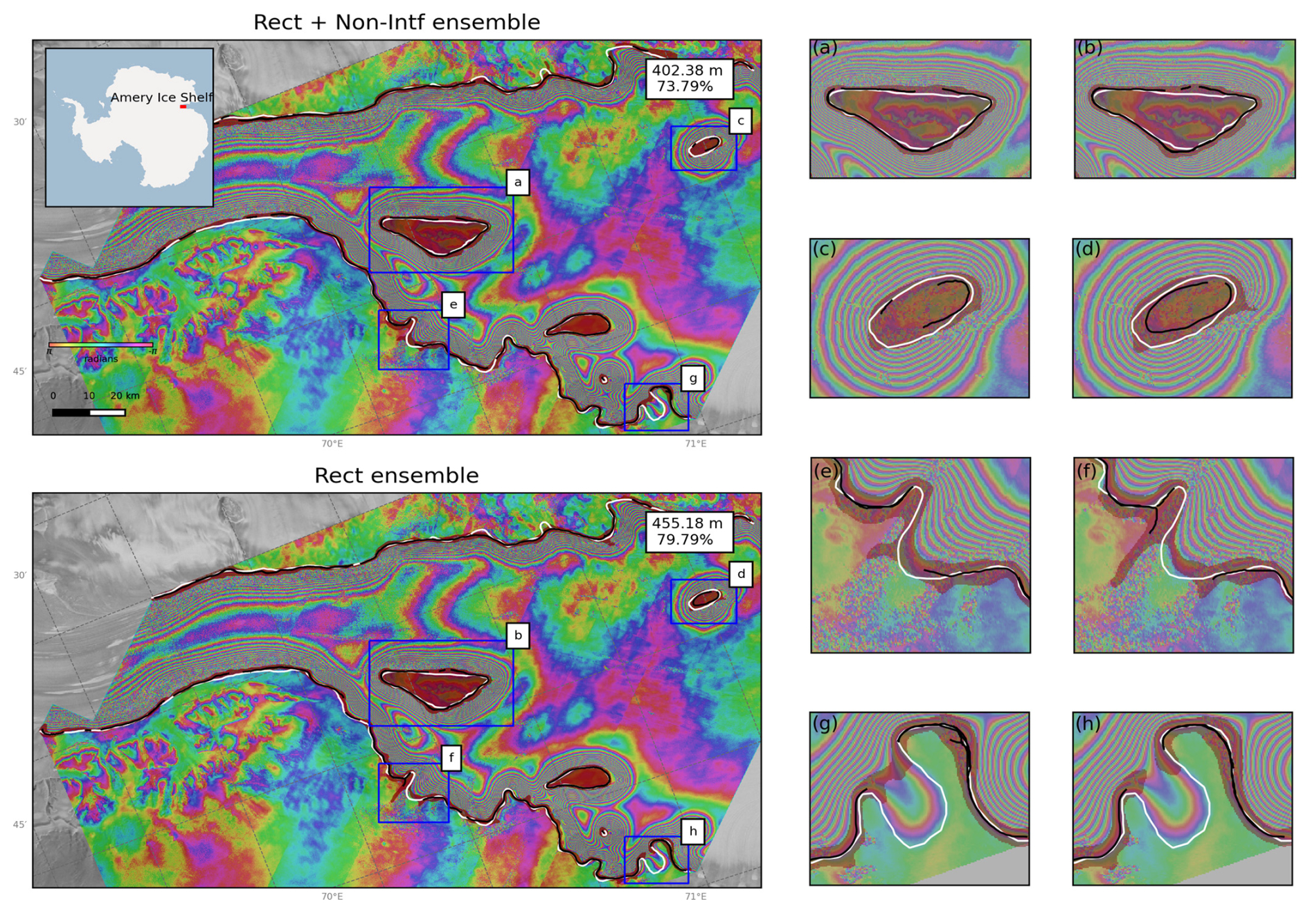
Figure 11 Manual GLs (white) and HED delineations of the ensemble networks (Table 5) (black) of the Amery Ice Shelf test sample. The predictive uncertainty is depicted as the shaded region enveloping the lines (red). The inset shows examples of regions where the width of the uncertainty buffer extends into features such as the (a, b) Clemence Massif and (c, d) Budd Ice Rumples. The models are also uncertain over (e, f) partially decorrelated fringes and (g, h) loose fringes.

5 Estimation of predictive uncertainty

We estimated the predictive uncertainty of our model by training an ensemble of five neural networks. We chose not to further decompose this uncertainty into data and model components, as there is no standardized approach for doing so (Gawlikowski et al., 2023). The ensemble approach is conceptually similar to the round-robin test used for manual delineations (Muir, 2020), wherein the GL delineation is repeated for each sample using multiple networks. Each network was initialized with a unique random seed, resulting in different initial weights and a randomized order of training samples (Lakshminarayanan et al., 2017). All networks were trained on the temporal dataset variant. For each sample, we computed the pixel-wise mean and standard deviation of the predicted probabilities (Fig. 10), and we converted the mean probabilities into mean GLs using the same postprocessing procedure described in Sect. 3.3.

Following the approach described in Tollenaar et al. (2024), we illustrate the spatial uncertainty of the models' predictions as a buffer around the ensemble average grounding line. This buffer was derived by adding one standard deviation to the mean prediction at each pixel, followed by binarizing the resulting values using a threshold of 0.8. We applied this procedure to two separate ensembles trained with feature subsets corresponding to networks 1 and 3 in Table 3. We quantified the spatial uncertainty across the test set by measuring the distance from the average GL to the nearest boundary of the uncertainty buffer at 10 km intervals along the mean GLs. We then computed the average of these distances to obtain a predictive error representative of the uncertainty. Table 5 summarizes the performance metrics for the two ensembles. Interestingly, the mean and median deviations of network 3 alone were better than those of the Rect + Non-Intf ensemble, though still within the uncertainty bounds. While ensemble methods often improve predictive accuracy, they do not always guarantee better results (Gawlikowski et al., 2023). However, the Rect ensemble performs better than network 1.

Figure 11 shows the average GLs derived from the two ensembles and the uncertainty buffer for a test sample. The buffer width indicates the degree of uncertainty. In most cases, the buffer extended symmetrically both landwards and seawards from the average GL. However, we observed wider buffers around small-scale features such as pinning points and massifs (Fig. 11a, b, c, d), decorrelated fringes (Fig. 11e, f), and loose fringes (Fig. 11g, h).

Finally, we evaluated the Antarctica-wide performance of the ensemble average GLs by comparing their PoLiS distances to AIS_cci lines (Fig. C4). Both ensembles exhibited particularly poor performance over the Antarctic Peninsula and the Totten Ice Shelf, likely due to the low coherence of the respective double-difference interferograms (Figs. C1 and 7).

6 Conclusions

We applied the HED deep neural network for automatically delineating grounding lines from DInSAR interferograms. The network was included as a module of our automatic GL delineation pipeline, which handles the preprocessing of DInSAR interferograms to make them suitable inputs for the network, trains the network to generate GL segmentation maps, and then applies postprocessing to obtain GL vector geometries. The network was trained on the AIS_cci GLL dataset, which consists of manually delineated GLs across several outlet glaciers and ice streams around the Antarctic Ice Sheet. Additional surface elevation data, ice velocity components, and differential tide levels were incorporated into the training stack to assess the influence of auxiliary features.

Our feature ablation experiments revealed that using the DEM improves GL detection, particularly in areas with poor coherence. However, since DEMs are derived from multiple SAR acquisitions over several years, they often do not align temporally with the SAR scenes used to build the double-difference interferogram, potentially resulting in erroneous delineations that deviate from the DInSAR fringe belt. Ice velocity and differential tide level features had a marginal positive effect when combined with the DEM, but their inclusion often resulted in sparse and spurious GL delineations. Consequently, we recommend using only the rectangular interferometric features for robust GL detection, minimizing the risk of introducing false positives. We provide an estimate of the networks' predictive uncertainty using an ensemble of networks. The standard deviation buffers largely extend over decorrelated fringes, indicating that the networks' predictions in such areas are not as reliable. The GLs from the Rect ensemble have 265 m median deviation and 421 m mean deviation from the AIS_cci GLLs as well as 401 m average predictive uncertainty.

Furthermore, we demonstrated that the trained HED network can delineate GLs from interferograms of previously unseen regions without retraining, enabling rapid processing of new interferograms without manual intervention. This adaptability makes the network suitable for large-scale GL migration studies across diverse timescales. Since our pipeline is agnostic to the SAR data source, it can be applied to DInSAR interferograms from various spaceborne SAR missions, including recent and upcoming missions such as Sentinel-1C and NISAR. This flexibility underscores the pipeline's potential to support long-term, automated GL monitoring across the Antarctic Ice Sheet.

Appendix A: Resampling wrapped phases

In order to conserve the cyclic variation of phase, the amplitude and phase of the double-difference interferograms were resampled separately. Due to missing SAR backscatter information for the interferograms used in the AIS_cci dataset, we used a unit amplitude component to obtain a complete complex polar representation of the interferograms. The polar components were transformed into real and imaginary parts (Fig. A1), which were resampled separately. These were transformed back to polar form to obtain resampled pseudo-coherence and phase information (Fig. A2).

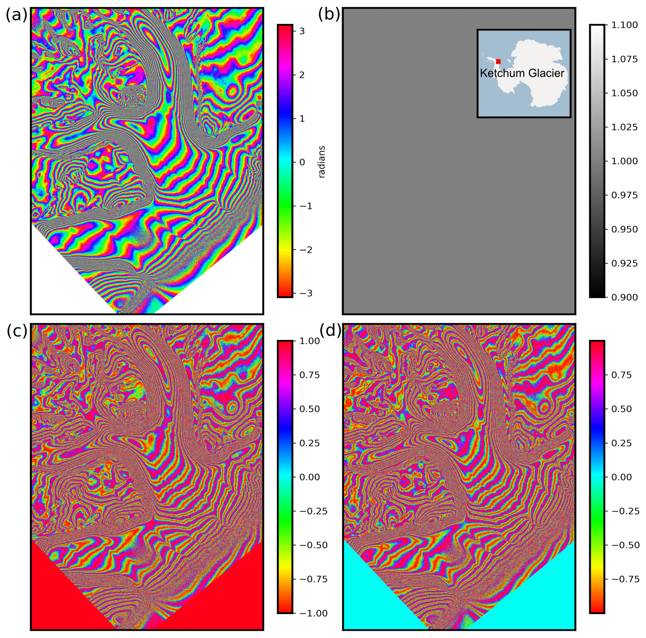
Figure A1 Phase-preserving reprojection and resampling scheme illustrated for (a) sample ERS interferogram of Ketchum Glacier in the Antarctic Peninsula and (b) the added unit amplitude component (both in EPSG:4326 projection). Transformation from polar components to (c) imaginary and (d) real components. The image extents in latitude and longitude were not set to prevent distorting the visualization.

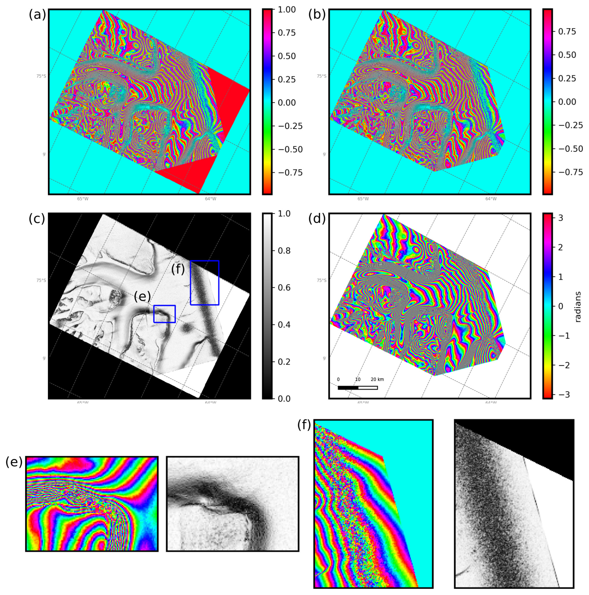
Figure A2 The resampled and reprojected (a) real and (b) imaginary interferometric components of the DInSAR phase sample shown in Fig. A1. Both were reprojected to EPSG:3031 projection with a pixel size of 100 m × 100 m. These components are transformed back to (c) pseudo-coherence and (d) phase. The insets in (c) show the variation of pseudo-coherence for the cases where (e) the phase is coherent but contains high-frequency fringes and (f) the phase is decorrelated. In both cases, the pseudo-coherence value is <0.4.

Appendix B: HED architecture diagram

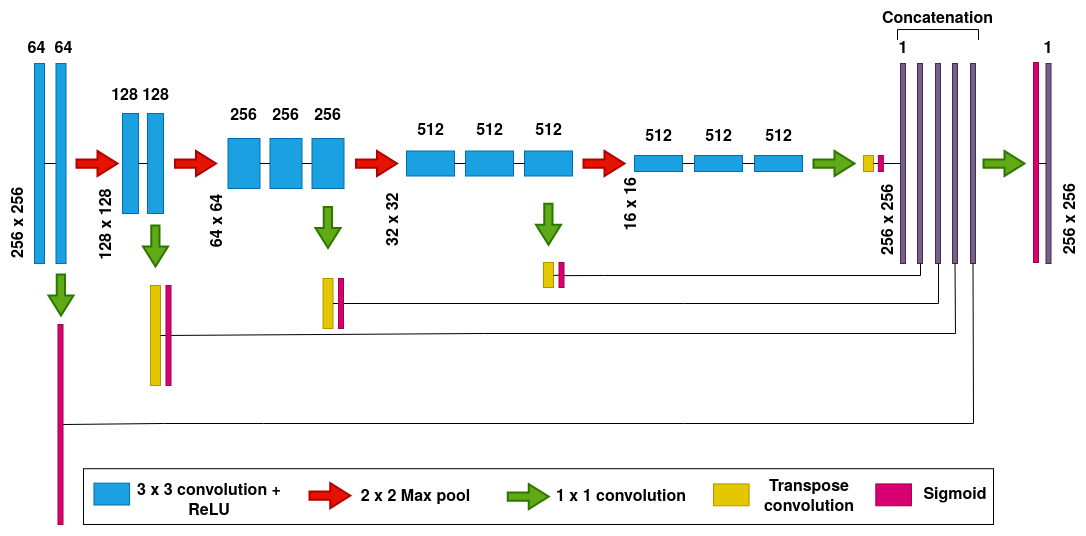
Figure B1 Architecture of the holistically nested edge detection neural network (Xie and Tu, 2015).

Appendix C: Additional results

The table below lists additional feature ablation experiments. The model trained with Vel + Tide features and the hyperparameters specified in Sect. 3.4 did not yield usable results and therefore were not used to compute metrics.

Table C1 Numerical results for networks trained with different feature subsets as described in Sect. 4.2. Abbreviations for feature subsets: Intf: interferometric features; DEM: digital elevation model; Vel: ice velocity (northing and easting components); Tide: differential tide level; Non-Intf: non-interferometric features.

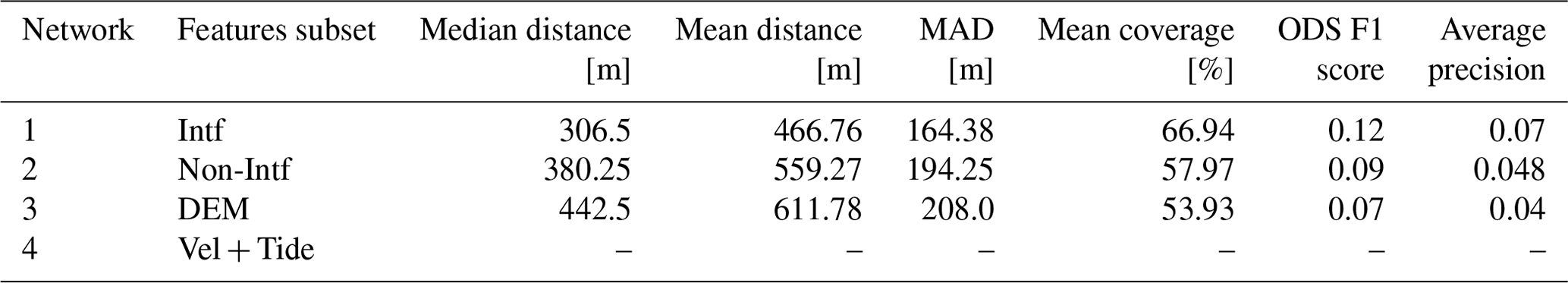
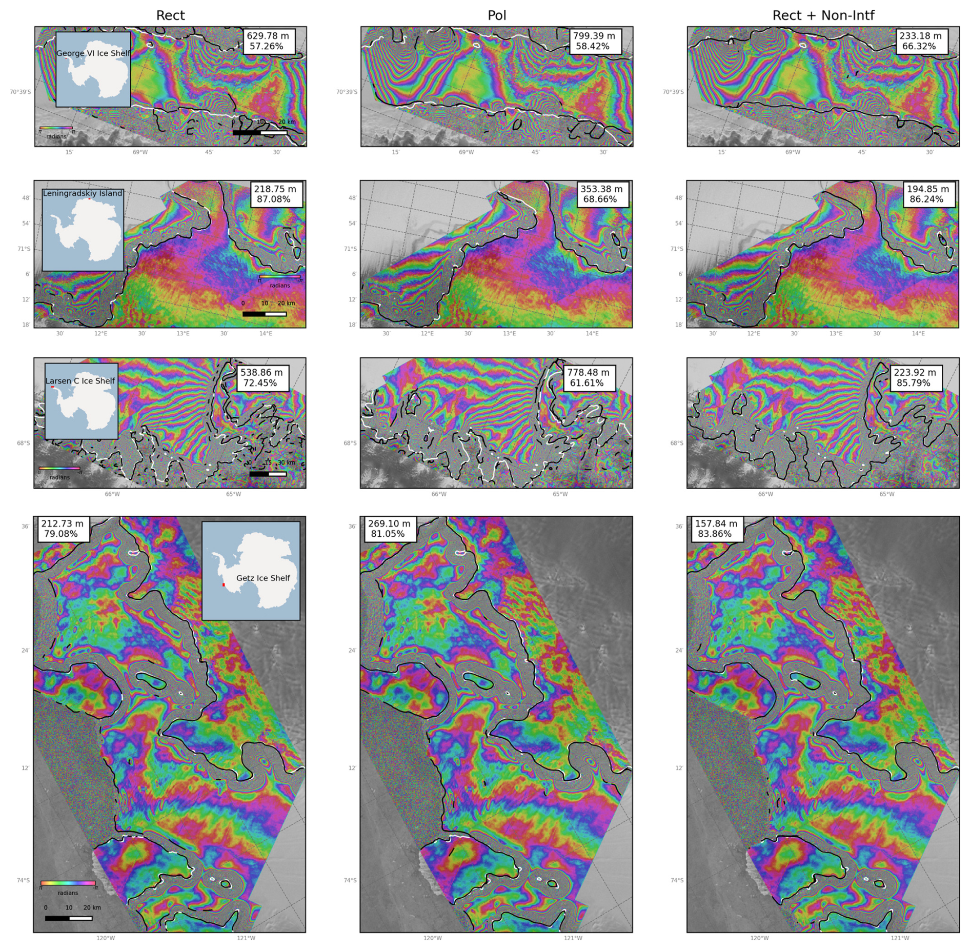
Figure C1 Visualization of the GLs generated by networks 1, 2, and 3 (Table 3) for several test samples.

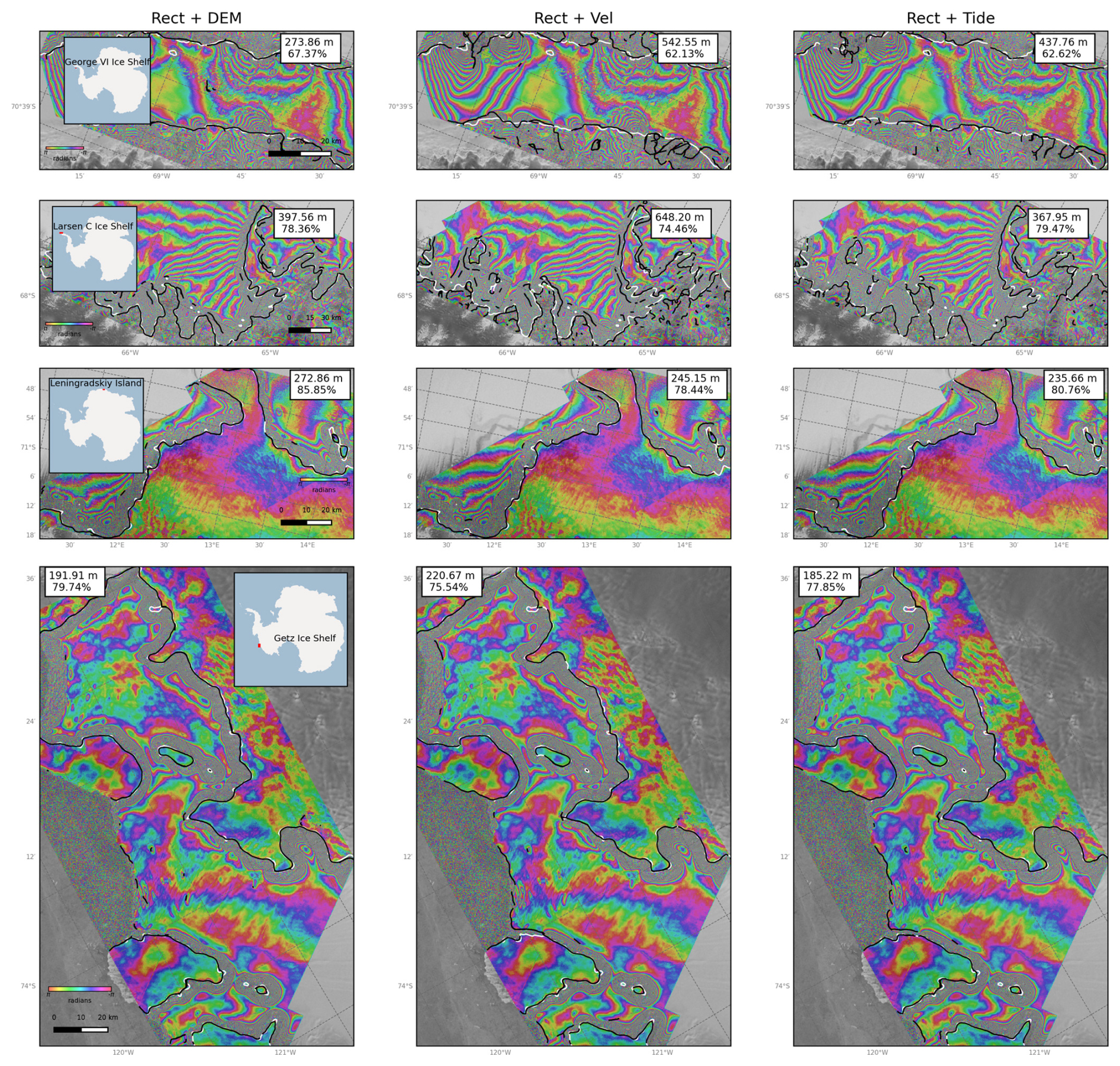
Figure C2 Visualization of the GLs generated by networks 4, 6, and 8 (Table 3) for several test samples.

Figure C3 Visualization of the GLs generated by networks 5, 7, and 9 (Table 3) for several test samples.

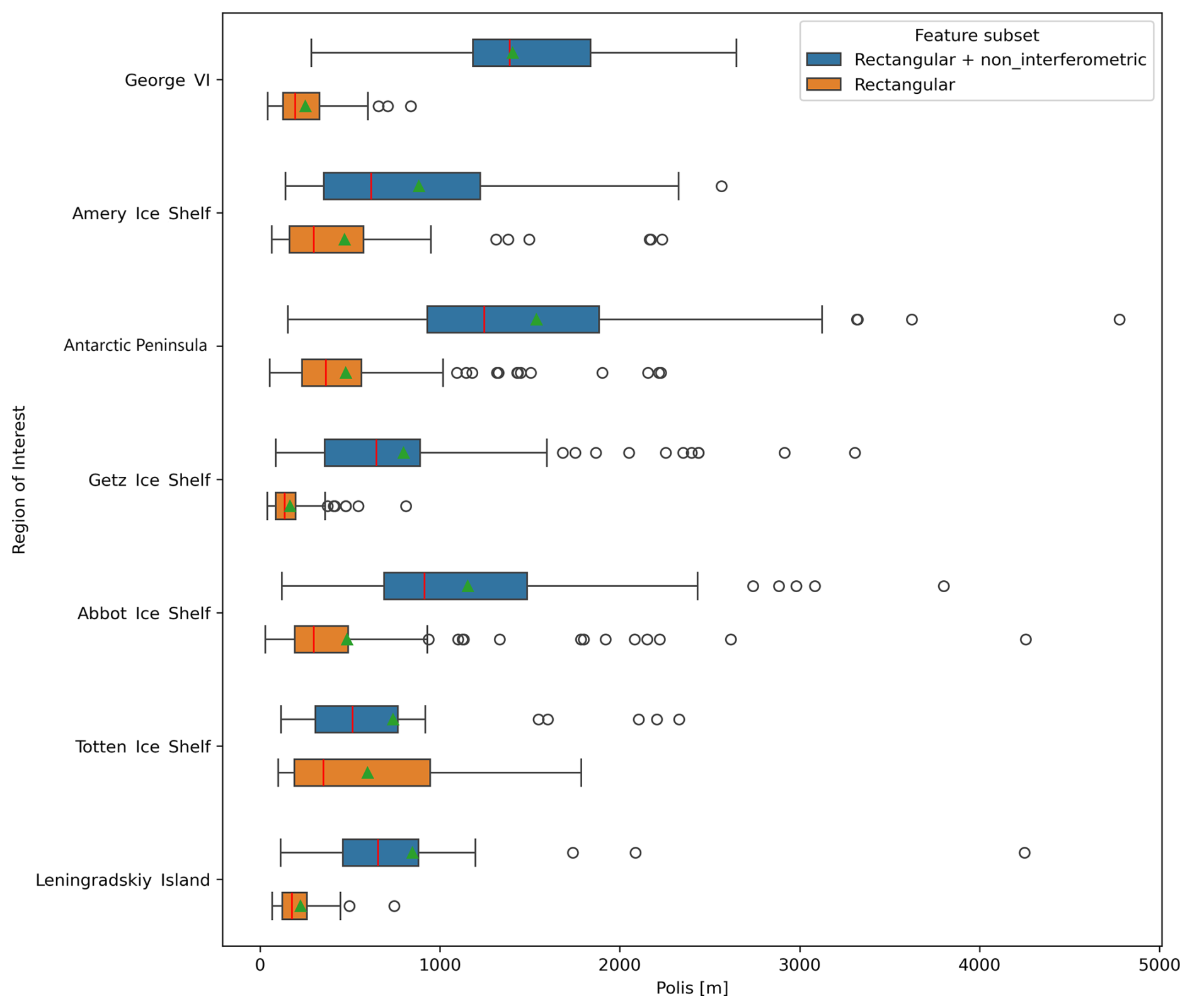
Figure C4 Region-wise performance of the two ensembles. The PoLiS distances shown here are for the test set of the temporal dataset variant. The green triangle and the red line indicate the mean and median distances, respectively. The circles outside the whiskers are outliers, which lie outside 1.5 times the interquartile range.