Improved basal drag of the West Antarctic Ice Sheet from L-curve analysis of inverse models utilizing subglacial hydrology simulations

The West Antarctic Ice Sheet (WAIS) is the focus of current research due to its susceptibility to collapse, which could potentially contribute to rising sea levels. To accurately predict future glacier evolution, precise ice sheet models are essential. The ice discharge of outlet glaciers into the ocean is one key factor here, primarily caused by the basal sliding of ice. Since we cannot directly measure basal properties on a large scale, inverse models can be used to infer the basal drag coefficient by minimizing a cost function that depends on a velocity misfit and a regularization term.

We conduct various basal drag inversions to obtain an improved basal drag distribution for the WAIS. Additionally, we perform L-curve analyses to determine the optimal trade-off between the cost function terms that result in smooth L-curves. The domain L-curve is divided into eight subdomains of the study area to assess how well the inverse method performs in different glaciological settings. Pine Island Glacier exhibits the smoothest L-curves, while slow-flowing regions such as Roosevelt Island reveal rather poorly shaped L-curve behavior for the basal drag inversion. This highlights the importance of performing a subdomain L-curve analysis for large-scale inversions to discover potential problematic regions and to establish suitable regularization for different physical conditions.

Comprehensive basal drag inversion experiments allow us to test the dependence of both the L-curves and the basal drag results on the nonlinearity of sliding and the inclusion of subglacial effective pressure in the friction law. The analysis suggests that nonlinear friction laws are preferable to linear sliding because of reduced variance in the overall inferred friction coefficient and steeper L-curves leading to a more well-defined corner region. We show that a Budd-type friction law that incorporates effective pressure from a subglacial hydrology model rather than a simple geometry-based approximation achieves improved performance in our inverse model in terms of the total model variance ratio, along with faster convergence and smoother L-curves. Further comparison reveals that the basal drag coefficient field has a less variable spatial structure when an effective pressure from the hydrology model is used instead of a parameterized effective pressure, allowing us to interpret the inverted drag coefficient more precisely in terms of the basal properties rather than the basal hydrology.

1 Introduction

The West Antarctic Ice Sheet (WAIS) experiences massive ice loss and is currently the major Antarctic contributor to sea-level change (Shepherd et al., 2018; Naughten et al., 2023). The instability of the WAIS and the related ongoing melt may lead to a future global sea-level rise of about 3.3 m (Bamber et al., 2009).

The ongoing development of ice sheet models (e.g., Blatter et al., 2010; Seroussi et al., 2019) is driven by advancements in research and the resulting improved understanding of ice sheet behavior. These improvements enhance our insights into key processes, such as ice dynamics and the ongoing melting. Consequently, more accurate initial states for ice sheet models can be established, further minimizing uncertainties in future projections (Seroussi et al., 2019). In the context of a deeper understanding of ice sheet processes and improved initial conditions, it is particularly important to examine friction distribution at the ice–bed interface. This process has a major influence on ice velocity, especially in fast-flowing areas (e.g., Engelhardt and Kamb, 1998), but cannot be measured on large scales. However, since remote sensing data, such as ice surface velocities, are available, the problem of determining the basal drag can be mathematically identified as an inverse problem. Solving such problems through optimal control methods can help to represent unknown parameters. The use of inversion techniques to infer the basal drag coefficient is a common approach within the glaciology community (MacAyeal, 1993; Joughin et al., 2004, 2009; Morlighem et al., 2010, 2013; Habermann et al., 2012; Sergienko and Hindmarsh, 2013; Sergienko et al., 2014; Zhao et al., 2018; Wolovick et al., 2023a).

To account for sliding beneath a glacier, a friction law (Weertman, 1957) is applied at the ice-base boundary condition of ice sheet models. The accuracy of the unconstrained parameters in this law plays an important role in modeling glaciers in realistic settings. In general, the friction law describes the basal drag as a function of basal velocity, the basal drag coefficient, and the influence of subglacial hydrology incorporated through effective (water) pressure (Budd et al., 1979). This emphasizes the relationship between glacier motion due to sliding at the base and subglacial hydrology (Cuffey and Paterson, 2010; Benn and Evans, 2010), as, simply put, the occurrence of water at the bed acts as a lubricant, facilitating sliding. Since effective pressure is thus a key component of the friction law, achieving a robust representation of subglacial hydrology is crucial for distinguishing basal properties driven by hydrological processes from those influenced by other factors. It is therefore desirable to use a more realistic and physically based representation of subglacial water pressure than has typically been done so far in the community (e.g., Werder et al., 2013; Flowers, 2015; Barnes and Gudmundsson, 2022; Dow, 2022; Kazmierczak et al., 2022; Ehrenfeucht et al., 2025). Here, we compare a commonly used parameterized effective pressure (e.g., McArthur et al., 2023; Wolovick et al., 2023a) with an effective pressure from a subglacial hydrology model (Sect. 2) to demonstrate the relevance of an improved description of water pressure.

In the inversion process, the basal drag coefficient is controlled by minimizing a cost function of the misfit between simulated and observed surface velocities. Due to the general ill-posedness of such inverse problems (Hadamard, 1902), it is difficult to solve these problems. Even small measurement errors in the observed surface velocities ${\mathit{v}}_{\text{s}}^{\text{obs}}$ can lead to significant and unrealistic artifacts in the unknown basal drag coefficient k. The integration of a regularization term (Tikhonov and Arsenin, 1977) in the cost function of the basal drag inversion ensures that unrealistic structures in the solution are smoothed by penalizing oscillations in the basal drag coefficient. To achieve a trade-off between the two cost function terms, it is necessary to determine a weight for the regularization term with the help of an L-curve (Hansen, 1992; Hansen and O’Leary, 1993; Hansen, 2001; Wolovick et al., 2023a). For this purpose, we follow Wolovick et al. (2023a) and perform an L-curve analysis that identifies the best weight for the regularized cost function term at the maximum curvature of the resulting L-shaped curve.

In the literature of the glaciological community, the regularization and the related L-curve analysis are not always applied when an inversion is performed (e.g., MacAyeal, 1993; Joughin et al., 2004, 2009; Arthern and Gudmundsson, 2010). Furthermore, we are not aware of any literature in which the basal drag inversion for the entire WAIS region (compare Fig. 1) is performed using both a regularization term and an explicit L-curve analysis (e.g., Joughin et al., 2004, 2009; Ranganathan et al., 2021). In addition, previous studies usually consider only individual glaciers or regions of the WAIS, such as Joughin et al. (2004), who focus on the Ross Ice Shelf; Ranganathan et al. (2021), who concentrate on MacAyeal Ice Stream; Morlighem et al. (2010) and Gillet-Chaulet et al. (2016), who deal with Pine Island Glacier; and Joughin et al. (2009) and Sergienko and Hindmarsh (2013), who examine both Pine Island Glacier and Thwaites Glacier. Although Morlighem et al. (2013) and Arthern et al. (2015) model the entire Antarctic ice sheet, the results of those studies are nevertheless not based on a high-resolution mesh. In the literature, instead of a Budd-type friction law (Budd et al., 1979), a Weertman friction law (Weertman, 1957) is often used (e.g. Morlighem et al., 2010, 2013; Joughin et al., 2004; Ranganathan et al., 2021) in which no effective pressure is taken into account. It is also common when using a Budd-type friction law to use a simple geometry-based parameterization for the effective pressure (e.g., Arthern et al., 2015; Barnes and Gudmundsson, 2022; Kazmierczak et al., 2022). As this parameterization is not ideal due to its strong simplifications of subglacial processes (e.g., a perfect connection to the ocean of marine parts of the ice sheet), it is desirable to leverage the results of hydrology models (e.g., Koziol and Arnold, 2017; Beyer et al., 2018; Gilbert et al., 2022; McArthur et al., 2023).

The disadvantage of inverse methods is the numerical instability, as all existing errors in the system are reflected in the unknown basal drag coefficient to be determined, which leads to an inaccurate result. These errors can, for example, be based on incorrect model physics, such as assumptions for the flow law regarding anisotropy, which can influence the ratio of deformation to sliding flow, as described in McCormack et al. (2022). Rathmann and Lilien (2022) point out that neglecting the crystal-orientation fabric in the flow law can influence the inferred basal drag coefficient, which can be remedied by including an isotropic enhancement factor and inverting both the rheology and the basal drag coefficient. In addition, the basal drag coefficient is sensitive to temperature assumptions and thus to the determination of ice rheology (Zhao et al., 2018). Kyrke-Smith et al. (2018) find that the accuracy of the bed elevation data affects the derived basal conditions, and they suggest inverting for both the basal drag coefficient and the basal topography. The importance of friction laws and thus the capture of subglacial hydrology contribute to a more realistic basal drag coefficient determined from inversions (Schroeder et al., 2013; McArthur et al., 2023). Overall, there are many assumptions behind every inversion of basal drag, as, for example, there are not necessarily enough data available or the aim of the studies differs. However, in this paper, we focus primarily on the choice of the friction law and the associated subglacial hydrology to reduce uncertainty in the resulting basal drag coefficient.

One objective of this paper is to test whether an improved description of the effective pressure results in a more reliable basal drag distribution for a major part of the WAIS. Therefore, we leverage the effective pressure from a physically based subglacial hydrology model in the friction law and apply the common basal drag inversion. We use the effective pressure of a confined–unconfined aquifer system model (CUAS-MPI; Beyer et al., 2018; Fischler et al., 2023), as it was shown to perform well in SHMIP (Subglacial Hydrology Model Intercomparison Project) (De Fleurian et al., 2018) and is able to describe different states of the water system. In addition, we conduct a subdomain L-curve analysis to explore how the regularization of the inverse problem varies with glaciological settings. Based on the simulations performed, we examine the basal drag distribution and analyze the influence of the different effective pressure maps, the linear and nonlinear friction law on the L-curve, and the spatial variability in the basal drag coefficient.

In the following paper, we firstly describe the methods and data that we use to perform the inversion for the WAIS (Sect. 2). We present our results regarding the spatial distribution of the basal drag and the basal drag coefficient, along with the L-curves obtained and the subdomain L-curve analysis (Sect. 3). Finally, we discuss our findings and compare them with other studies (Sect. 4).

2 Methods

In the following subsections, we describe the ice flow model setup for the study region covering the WAIS. Subsequently, we present the forward model and the inversion process, including regularization and the L-curve analysis.

2.1 Model setup

Our simulations are conducted within the open-source, finite-element-based Ice-sheet and Sea-level System Model (ISSM; Larour et al., 2012). In total, we perform six basal drag inversions with an accompanying L-curve experiment (compare Sect. 3). The experiments encompass setups with linear and nonlinear sliding for both Weertman- and Budd-type friction laws. To evaluate the impact of varying effective pressure fields, we either set this field to an effective pressure from the subglacial hydrology of CUAS-MPI, apply a simple geometry-based parameterization, or neglect the effective pressure entirely.

Application to the West Antarctic Ice Sheet

We choose the WAIS domain (Fig. 1) by using the defined ice sheet drainage basins of Rignot (Glovinetto and Zwally, 2000; Rignot et al., 2011a, c, 2013) from the Ice Sheet Mass Balance Inter-comparison Exercise (IMBIE-3; Rignot et al., 2019). As ice shelves are not included in those basins, we include them with the MEaSUREs Antarctic Boundaries dataset (Mouginot et al., 2017). We exclude the so-called J-Jpp basin describing the Filchner–Ronne catchment to keep the computational effort at a manageable level. However, results of the basal drag of the J-Jpp basin have already been published by Wolovick et al. (2023a), which we do not aim to reproduce. We simulate the basins for Marie Byrd Land and Ellsworth Land without the Weddell Sea Sector. For the sake of simplicity, we will nevertheless refer to it as the WAIS in the following.

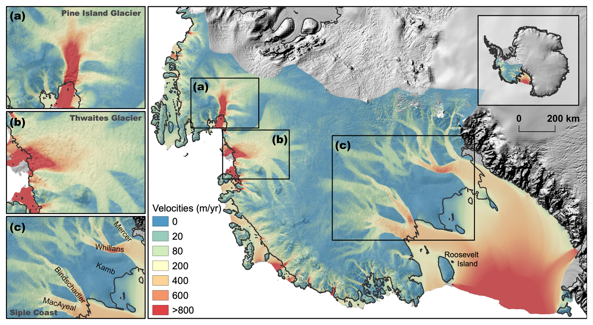
Figure 1 Map of the study domain covering a large part of the WAIS. The plots show the observed surface velocities (in m yr⁻¹) from the MEaSUREsv2 dataset (Rignot et al., 2011b, 2017). The background imagery displays the ice surface elevation of Antarctica from the BedMachine Antarctica v2 dataset (Morlighem et al., 2020; Morlighem, 2020). The black line represents the grounding line. Insets (a), (b), and (c) show zoom-ins to Pine Island Glacier, Thwaites Glacier, and the Siple Coast (with the Mercer, Whillans, Kamb, Bindschadler, and MacAyeal ice streams), respectively.

Figure 1 illustrates that we are dealing with both slow- and fast-flowing areas in this domain, including Thwaites Glacier, Pine Island Glacier, and the Siple Coast ice streams. In Fig. 2a, the bed elevation is displayed and clearly shows that most of the WAIS area lies below sea level with the interior deeper than the margins, making it vulnerable to marine ice sheet instability (e.g., Hughes, 1973; Weertman, 1974; Thomas and Bentley, 1978; Schoof, 2007). The geometry is based on the BedMachine Antarctica v2 dataset (Morlighem et al., 2020; Morlighem, 2020). This dataset includes bed topography (Fig. 2a), surface elevation (Fig. 2b), ice thickness (Fig. 2c), and the mask for the WAIS (Fig. 2f).

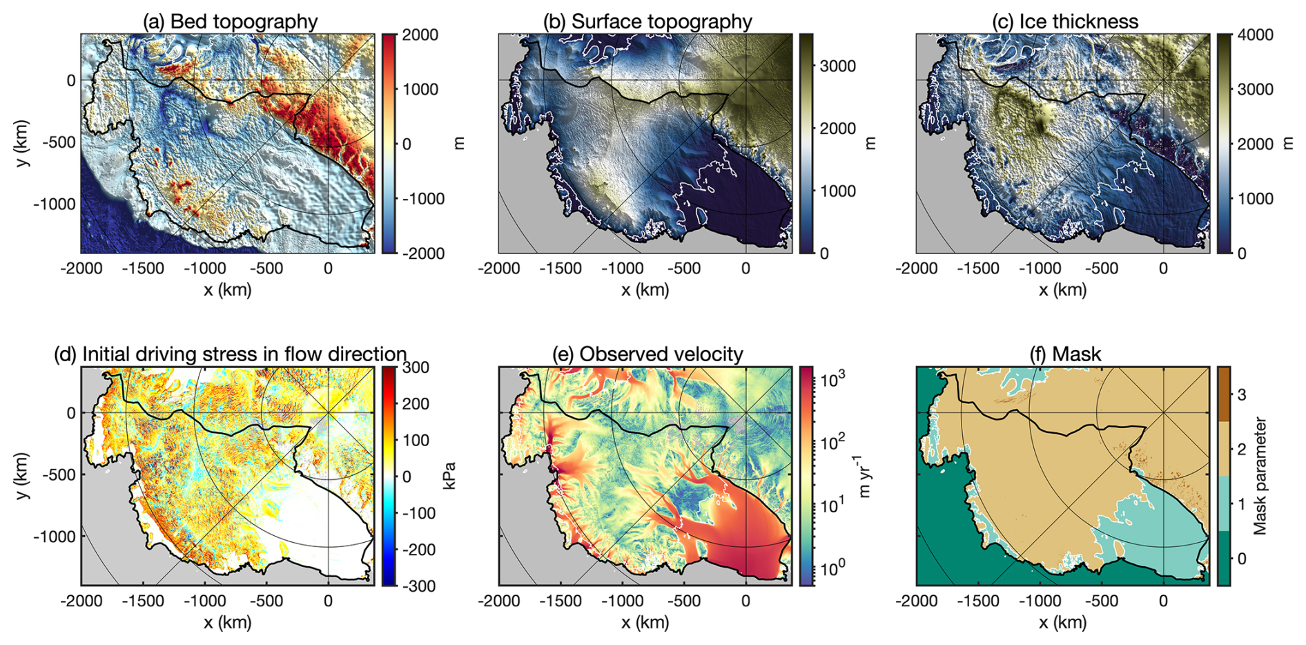
Figure 2 Model setup of the WAIS domain. (a) Bed topography (in m). (b) Surface elevation (in m). (c) Ice thickness (in m). (d) The initial driving stress in flow direction (in kPa). (e) Observed surface velocity (in m yr⁻¹) in log scale from the MEaSUREsv2 dataset (Mouginot et al., 2012; Rignot et al., 2011b, 2017). (f) WAIS mask, with mask parameter 0 describing the ocean, mask parameter 1 describing the floating ice, mask parameter 2 describing the grounded ice, and mask parameter 3 describing exposed rock. Subplots (a)–(d) and (f) are based on the BedMachine Antarctica v2 dataset (Morlighem et al., 2020; Morlighem, 2020). The white line in the subplots describes the grounding line, and the black line delineates the study area. Plots (a)–(c) are overlaid on a hillshade background. Gray areas in panels (d)–(e) indicate regions with no available data.

Mesh construction

We construct a two-dimensional (2D) unstructured triangular mesh generated by using the Bidimensional Anisotropic Mesh Generator (BAMG; Hecht, 2006). The horizontal mesh is refined in dynamic active regions, such as the shear margins (Fig. 3a), the calving front, fast-flowing areas and outlet glaciers, and the grounding line. The mesh is extruded into 10 vertical layers so that we get a three-dimensional prism structure of the mesh.

The overall procedure to generate the mesh is based on a control field construction as described in Wolovick et al. (2023a). In Fig. 3, the underlying control field for the horizontal mesh generation and the element sizes are shown. The control field (Fig. 3a) indicates the basis of the refinement strategy. For example, we want to achieve a high resolution where the ice flow is fast, demonstrated by the yellow areas in Fig. 3a, such as at the grounding line. The mesh resolution (Fig. 3b) is relatively low in the slow-flowing regions with around 15 km resolution, and the largest elements have a resolution of 20 km. The red and orange areas indicate a high resolution between 500 m and 1 km, exactly where the grounding line and the shear margins are located. This resolution is a factor of about 3–6 higher than in Morlighem et al. (2013) (they use 3 km) and a factor of about 5–10 higher than in Arthern et al. (2015) (they use 5 km for the whole domain of Antarctica). Overall, the resulting mesh consists of 417 284 2D elements. At the end of the meshing procedure, all relevant gridded data, such as the bed topography (Fig. 2a), the ice thickness (Fig. 2c), the observed surface velocities (Fig. 2e), and the mask (Fig. 2f), are interpolated with a multi-wavelength interpolation introduced in Wolovick et al. (2023a) onto the mesh.

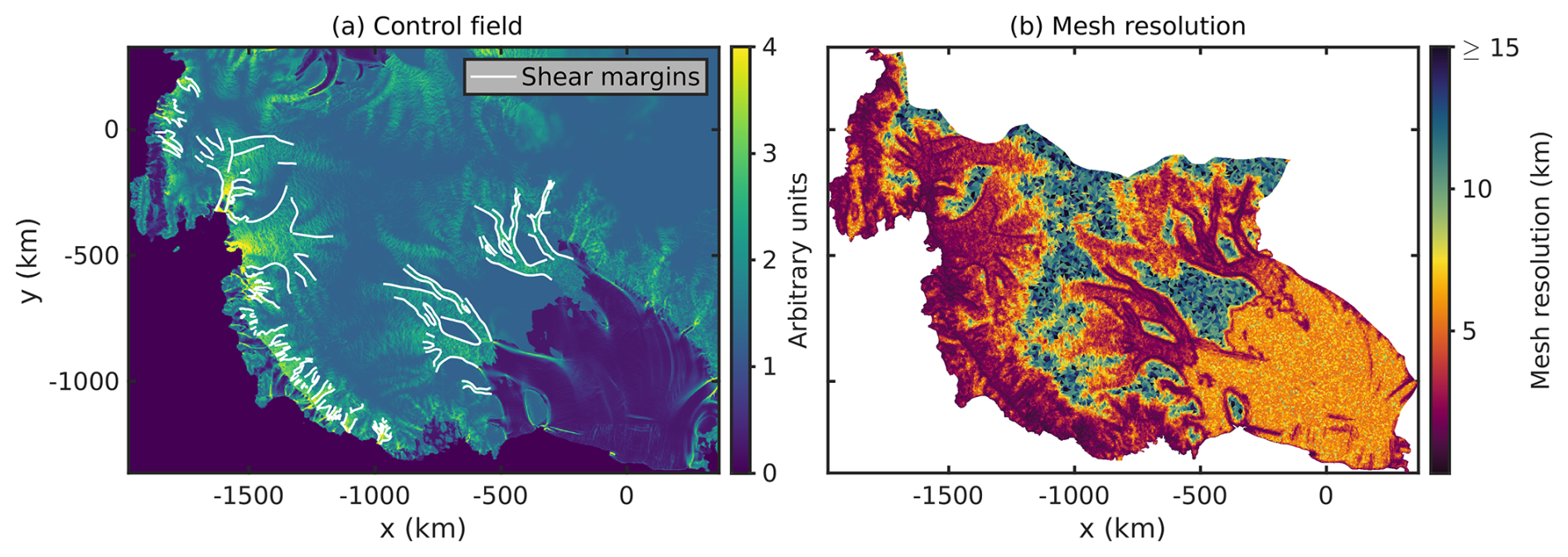
Figure 3 Maps of mesh characteristics. (a) The control field used to guide the spatial pattern of mesh refinement. The white lines indicate the detected shear margins, which are also used to create the mesh through refinement at this position. (b) The resolution of the mesh with different element sizes ranges from 500 m to ∼19 km.

2.2 Forward model

We use a forward model that represents the ice dynamics in an approximated way and is explained by the following higher-order (HO) Blatter–Pattyn approximation (Blatter, 1995; Pattyn, 2003) that computes the horizontal ice velocities v_x,v_y.

$$\begin{array}{}\text{(1)}& \begin{array}{rl}& {\displaystyle \frac{\partial }{\partial x}}\left(\mathrm{4}\mathit{\eta }{\displaystyle \frac{\partial v_x}{\partial x}}+\mathrm{2}\mathit{\eta }{\displaystyle \frac{\partial v_y}{\partial y}}\right)+{\displaystyle \frac{\partial }{\partial y}}\left(\mathit{\eta }{\displaystyle \frac{\partial v_x}{\partial y}}+\mathit{\eta }{\displaystyle \frac{\partial v_y}{\partial x}}\right)+{\displaystyle \frac{\partial }{\partial z}}\left(\mathit{\eta }{\displaystyle \frac{\partial v_x}{\partial z}}\right)\\ & ={\mathit{\rho }}_{\text{i}}g{\displaystyle \frac{\partial h_{\text{s}}}{\partial x}}\\ & {\displaystyle \frac{\partial }{\partial x}}\left(\mathit{\eta }{\displaystyle \frac{\partial v_x}{\partial y}}+\mathit{\eta }{\displaystyle \frac{\partial v_y}{\partial y}}\right)+{\displaystyle \frac{\partial }{\partial y}}\left(\mathrm{4}\mathit{\eta }{\displaystyle \frac{\partial v_y}{\partial y}}+\mathrm{2}\mathit{\eta }{\displaystyle \frac{\partial v_x}{\partial x}}\right)+{\displaystyle \frac{\partial }{\partial z}}\left(\mathit{\eta }{\displaystyle \frac{\partial v_y}{\partial z}}\right)\\ & ={\mathit{\rho }}_{\text{i}}g{\displaystyle \frac{\partial h_{\text{s}}}{\partial y}}\end{array}\end{array}$$

The density of ice is denoted by ρ_i, g represents the acceleration of gravity, h_s is the surface elevation of the glacier, and η is the ice viscosity. The latter is described by the constitutive material law for ice, Glen's flow law (Glen, 1953):

$$\begin{array}{}\text{(2)}& \mathit{\eta }={\displaystyle \frac{B}{\mathrm{2}{\dot{\mathit{\epsilon }}}_e^{\frac{n-\mathrm{1}}{n}}}},\end{array}$$

where B is the ice rheology parameter, ${\dot{\mathit{\epsilon }}}_e=\sqrt{\frac{\mathrm{1}}{\mathrm{2}}\text{tr}\left({\dot{\mathit{ϵ}}}_{ij}^{\mathrm{2}}\right)}$ is the effective strain rate (with ${\dot{\mathit{ϵ}}}_{ij}$ as the strain-rate tensor), and n=3 is the flow exponent. The temperature is computed by using a one-dimensional (1D) vertical steady-state advection–diffusion thermal model as described in Wolovick et al. (2023a). To force this model, we use surface temperatures (Comiso, 2000), accumulation rates (mean of Van De Berg et al., 2005, and Arthern et al., 2006), and a geothermal heat flow (sum of Martos et al., 2017, and calculated shear heating). Subsequently, we compute the flow-rate factor B (Cuffey and Paterson, 2010).

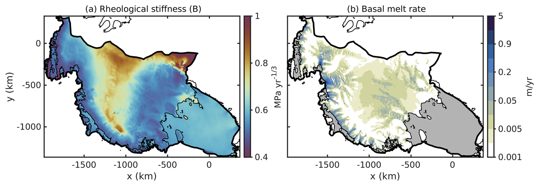
Figure 4 Results of the 1D steady-state advection–diffusion thermal model. (a) Vertically averaged ice rheology parameter B. (b) The basal melt rate of grounded ice is represented with a pseudo-log scale, with gray areas representing the floating ice. The thicker black line denotes the study area, and the thinner black line represents the grounding line.

Boundary conditions are given at the ice–atmosphere Γ_s, ice–bed Γ_b, and ice–margin Γ₋ interfaces to constrain the forward model. Towards the ice–atmosphere Γ_s, a traction-free homogeneous Neumann boundary is assumed. The lateral ice–margin boundary Γ₋ is constrained by an in-homogeneous Dirichlet condition in terms of observed surface velocities $\mathit{v}={\mathit{v}}_{\text{s}}^{\text{obs}}$. At the ice–bed interface Γ_b, we employ a friction law acting beneath the ice sheet. This friction law includes the unknown basal drag coefficient k, which we want to determine with our inversion approach. In ISSM, the basal friction law is implemented in terms of basal drag τ_b as

$$\begin{array}{}\text{(3)}& {\mathit{\tau }}_{\text{b}}=-k^{\mathrm{2}}{N}^r\left|\right|{\mathit{v}}_{\text{b}}|{|}_{\mathrm{2}}^{\frac{\mathrm{1}-m}{m}}{\mathit{v}}_{\text{b}}.\end{array}$$

Here, v_b is the basal velocity, m is the friction law exponent, r is the effective pressure exponent, and $N=p_{\text{i}}-p_{\text{w}}$ denotes the effective pressure as a function of ice pressure p_i and water pressure p_w. If the exponent of the effective pressure is r=0, i.e., N is neglected in Eq. (3), we obtain a Weertman-type friction law (Weertman, 1957). Otherwise, if r>0, the Budd-type friction law is applied. For m=1, the law is linear concerning velocity, whereas, for m>1, it becomes nonlinear in velocity. Throughout the study, we set r=0 when a Weertman sliding law is used and denote the corresponding basal drag coefficient k_W. We assign r=1 when a Budd-type sliding law is employed and denote the related basal drag coefficient k_B. We carry out experiments with these sliding laws, considering both linear sliding (i.e., m=1) and nonlinear sliding (i.e., m=3). Details on the effective pressure N are provided later in this subsection.

Our nonlinear forward model (Eq. 1) is solved with a Picard iteration scheme (iterative fixed-point method; Hindmarsh and Payne, 1996; Smedt et al., 2010) implemented in ISSM. The remaining linear systems of equations are solved with an iterative generalized minimal residual (GMRES) algorithm (Saad and Schultz, 1986) combined with a block Jacobi preconditioner provided by PETSc (Balay et al., 1997, 2019).

Subglacial hydrology

In the following, we compare a parameterized effective pressure N:=N_op against one from a hydrology model N:=N_CUAS. The effective pressure N_op is described by $N_{\text{op}}=p_{\text{i}}-p_{\text{w}}={\mathit{\rho }}_{\text{i}}gH-{\mathit{\rho }}_{\text{w}}g(-h_{\text{b}})$ assuming a perfect hydrological connection to the ocean, depending on the ice thickness H, the bed topography h_b, and the water density ρ_w. Note that we allow a negative water pressure.

To overcome shortcomings in the effective pressure parameterizations, we leverage the simulated effective pressure N_CUAS from the MPI parallel version of the confined–unconfined aquifer system model (CUAS-MPI; Beyer et al., 2018; Fischler et al., 2023). The model is based on an effective porous media approach (single-layer Darcy-type flow) and solves an evolution equation for the hydraulic head:

$$\begin{array}{}\text{(4)}& h={\displaystyle \frac{p_{\mathrm{w}}}{{\mathit{\rho }}_{\mathrm{w}}g}}+h_{\mathrm{b}}+z_{\mathrm{w}},\end{array}$$

where ρ_w is the density of water and $\mathrm{0}\le z_{\mathrm{w}}\le b$ is the elevation within the aquifer of thickness b. The hydraulic transmissivity is spatially and temporally varying and evolves due to channel wall melt, creep closure, and cavity opening. This makes it possible to simulate both inefficient and efficient water transport without resolving individual channels. The ice sheet geometry for the hydrology model is also based on the BedMachine v2 dataset but is cropped out for the area shown in Fig. 2 and interpolated onto a 1 km regular grid. CUAS-MPI also needs a mask to distinguish between active points and boundary conditions. This mask is based on the interpolated bed elevation and ice thickness datasets from BedMachine, taking into account the floating condition. No-flow boundary conditions are used along the grounded part of the basin delineation (black line in Fig. 2) and next to ice-free land (mostly rock outcrops). To avoid water flowing into areas that are most likely to be frozen to the bed, no-flow conditions are imposed in areas where the ice thickness is below 10 m or the bed elevation is 2000 m above sea level. At the ocean boundary, a Dirichlet condition (h=0 m) is applied. We initialize the head so that the water pressure is 90 % of the ice overburden pressure.

The subglacial hydrology model is forced with the steady but spatially variable ice sheet basal melt distribution (Fig. 4b) based on the 1D vertical steady-state advection–diffusion thermal model that is also used for rheology B (Fig. 4a) in the ISSM model setup (compare Sect. 2.2). Figure 4a reveals a belt in the center of the study area that exhibits increased ice stiffness associated with low surface temperatures (not shown here) and high surface elevations (compare Fig. 2b). In contrast, we can observe relatively soft ice at the margins of the domain, where warm surface temperatures and lower surface elevations predominate. The thermal model suggests that about 30 % of the rectangular CUAS-MPI domain enclosing the study area in Fig. 4b is frozen to the bed. The basal melt rate in Fig. 4b reflects the velocity field, which is reasonable, as it is included in the computation of the melt rates. The relatively high values of basal melt rate result from high rates of shear heating. High melt rates ($>\mathrm{0.5}\mathrm{m}{\mathrm{yr}}^{-\mathrm{1}}\mathrm{w}.\mathrm{e}.$) are located close to the grounding line of Pine Island Glacier and Thwaites Glacier, but those areas cover only about 0.2 % of the total warm-based area. Most of the melt rates are in the millimeter range (median: $\sim \mathrm{6}\mathrm{mm}{\mathrm{yr}}^{-\mathrm{1}}\mathrm{w}.\mathrm{e}.$) and clearly show the fast-flowing areas.

We run the model with 1 h time steps for 10 years using the same model parameters as in Beyer et al. (2018, Table 1 and Table 3), except we use an aquifer of thickness 1 m and a smaller minimum transmissivity ($T_{\min }={\mathrm{10}}^{-\mathrm{14}}{\mathrm{m}}^{\mathrm{2}}{\mathrm{s}}^{-\mathrm{1}}$).

Since we did not apply CUAS-MPI to ice rises, we set N_CUAS to the hydrostatic pressure N_op. In addition, the rock outcrops shown in Fig. 2f need special treatment, as they do not contain data entries. We interpolate over them on the CUAS-MPI grid. Finally, we interpolate the mentioned regions to the finite-element mesh. Since Thurston Island is not included in the CUAS-MPI model domain, we set the effective pressure at this site to ice pressure p_i and neglect the water pressure p_w due to the predominating low velocities at this location.

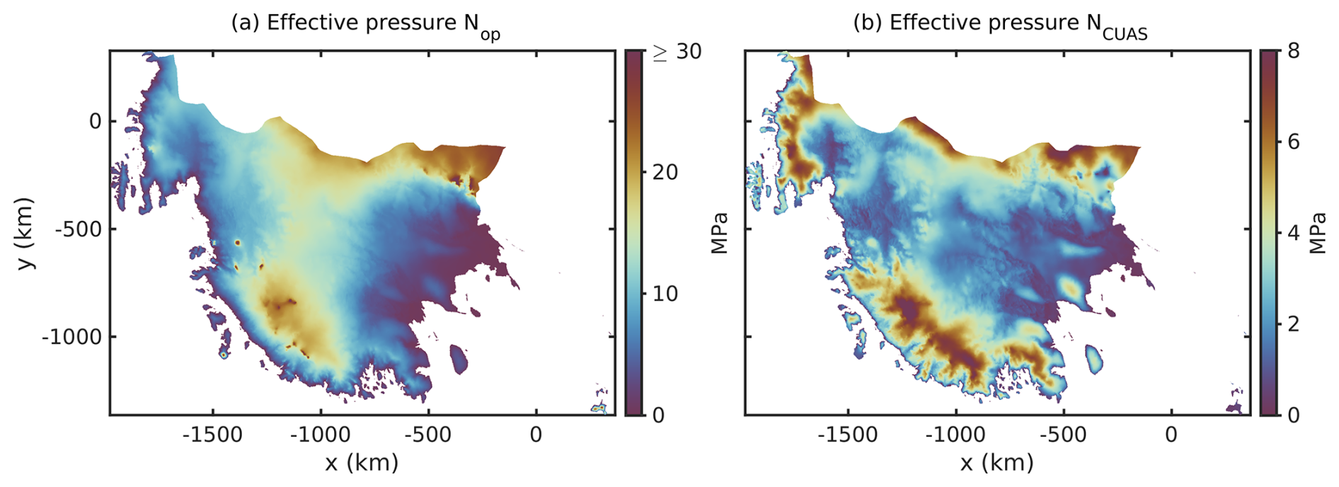
Figure 5 Effective pressure distributions for the WAIS. (a) Geometry-based effective pressure N_op ranging from 0 to 36 MPa. (b) Effective pressure N_CUAS based on the results from the subglacial hydrology model CUAS-MPI ranging from 0 to 8 MPa, including the modifications for areas that are not part of the CUAS-MPI domain.

The effective pressures N_op and N_CUAS are displayed in Fig. 5. In contrast to N_CUAS (Fig. 5b), the simple parameterization of the effective pressure N_op (Fig. 5a) reaches a much higher magnitude of 30 MPa in the slow-flowing areas of the domain than the effective pressure N_CUAS ranging only up to 8 MPa. Furthermore, the structure of the effective pressure from the subglacial hydrology model N_CUAS shows a similar distribution to the velocity field (compare Fig. 1), as expected.

2.3 Basal drag inversion

Parameter identification problems occur in ice sheet modeling because some relevant parameters are difficult to observe directly, such as the distribution of the basal drag underneath the ice sheets. These problems are referred to as inverse problems in the sense that we want to infer from an observed effect of a system the underlying but not measurable cause. In ice sheet models, this can be represented through the observed ice surface velocities as the observed effect from which we determine the unknown basal drag coefficient. This demonstrates that the most relevant data for the inversion procedure to fit the modeled horizontal ice velocities v_x,v_y are the observed ice surface velocities ${\mathit{v}}_{\text{s}}^{\text{obs}}$. Here, we use the ice surface velocities of the MEaSUREs v2 dataset (Mouginot et al., 2012; Rignot et al., 2011b, 2017) as the target of the inversion because it provides complete spatial coverage within the modeling domain (Fig. 2e).

In glaciology, such inverse problems can be described by minimizing a cost function (Eq. 5) while satisfying the underlying forward model (Eq. 1) and controlling the unknown basal drag coefficient k:

$$\begin{array}{}\text{(5)}& \begin{array}{rl}\underset{k}{min}{J}_{\text{raw}}\left({\mathit{v}}_{\text{s}},k\right)& =\underset{{\mathrm{\Gamma }}_{\text{s}}}{\int }{\displaystyle \frac{\mathrm{1}}{\mathrm{2}}}({\left(v_x-v_x^{\text{obs}}\right)}^{\mathrm{2}}+{\left(v_y-v_y^{\text{obs}}\right)}^{\mathrm{2}})\mathrm{d}{\mathrm{\Gamma }}_{\text{s}}\\ & +\mathit{\lambda }\underset{{\mathrm{\Gamma }}_{\text{b}}}{\int }{\displaystyle \frac{\mathrm{1}}{\mathrm{2}}}\left|\right|\mathrm{\nabla }k|{|}_{\mathrm{2}}^{\mathrm{2}}\mathrm{d}{\mathrm{\Gamma }}_{\text{b}}.\end{array}\end{array}$$

The first term of Eq. (5) describes the absolute velocity misfit, with ${\mathit{v}}_{\text{s}}^{\text{obs}}=(v_x^{\text{obs}},v_y^{\text{obs}})$ as the observed ice surface velocity, ${\mathit{v}}_{\text{s}}=(v_x,v_y)$ as the modeled ice velocity, and k as the respective control parameter for the inversion. We restrict our cost function to an absolute misfit term and opt against using a logarithmic misfit, as applied by Morlighem et al. (2013), since we do not perform a rheological inversion (see Sect. 4 for details). To improve the instability of the inverse problem, it is beneficial to add regularization. Therefore, the second summand is added to the cost function (Eq. 5), describing a typical Tikhonov regularization term (Tikhonov and Arsenin, 1977) by penalizing oscillations in the basal drag coefficient k. This additional term is equipped with a weight λ, which can be derived by performing an L-curve analysis. An L-curve analysis is meant to be a trade-off curve between the first cost function term J_raw,obs and the regularization term J_raw,reg. The idea behind conducting an L-curve analysis is to pick the best weight λ in the corner of the L shape.

For the L-curve analysis, we consider a range of λ covering 6 orders of magnitude (Sect. 4.1) with 25 logarithmically spaced samples. A basal drag inversion is performed for each sample, and the resulting costs J_obs and J_reg are recorded. To avoid arbitrarily selecting the best λ_best value by handpicking, we generate a smoothed L-curve using the 25 sample results in the (ln (J_reg),ln (J_obs)) space and determine the λ_best value by calculating the maximum curvature (second derivative), following the method of Wolovick et al. (2023a). Smoothing is required in this case because the second derivative tends to amplify noise. The smoothed trade-off curve is obtained by subsampling the 25 model results into 1000 logarithmically spaced λ subsamples. Subsequently, 50 different smoothing wavelengths are tested to identify the optimal one in the ln (λ) space through a sort of meta-regularization. Therefore, we calculate the variance for each wavelength based on the curvature of the smoothed curve and the scatter of the original model points. For further details on the variance calculation, see Wolovick et al. (2023a). The wavelength that minimizes the sum of both normalized variances is selected. The total logarithmic curvature $\frac{d^{\mathrm{2}}\left(ln\right(J\left)\right)}{d^{\mathrm{2}}\left(\ln \right(\mathit{\lambda }){)}^{\mathrm{2}}}$ is calculated, and the location of maximum curvature, representing the sharpest corner, identifies the λ_best value of the L-curve. The curvature is also recorded when it drops to half (arbitrary value) of the maximum value, providing a complete bracketed range from the minimum acceptable λ_min to the best-value λ_best and the maximum acceptable λ_max.

Moreover, the initial guess of the basal drag coefficient k impacts the convergence of the inversion (compare convergence criteria in Eq. 9). Therefore, it must be well quantified. A good approximation for the initial basal drag coefficient k_init can be computed from the driving stress and the observed ice velocity, e.g., as in Morlighem et al. (2013):

$$\begin{array}{}\text{(6)}& k_{\text{init}}={\left({\displaystyle \frac{max(\mathrm{0},{\mathit{\tau }}_{\text{d}})}{N\left|\right|{\mathit{v}}_{\text{s}}^{\text{obs}}|{|}_{\mathrm{2}}^{\mathrm{1}/m}}}\right)}^{\mathrm{1}/\mathrm{2}},\end{array}$$

where ${\mathit{\tau }}_{\text{d}}=-{\mathit{\rho }}_{\text{i}}gH\mathrm{\nabla }{h}_{\text{s}}\cdot {\mathit{v}}_{\text{s}}^{\text{obs}}/\left|\right|{\mathit{v}}_{\text{s}}^{\text{obs}}|{|}_{\mathrm{2}}$ describes the driving stress in flow direction. In the case of Weertman friction, N is set to 1 in Eq. (6), and, for the Budd-type friction law, a minimum value of 100 Pa is used. For velocity, we use a minimum value of 0.1 m yr⁻¹ to also prevent division by zero.

Following Wolovick et al. (2023a) again, we introduce a characteristic scale to normalize our cost function in Eq. (5) before we carry out the inversion procedure as described above. This is important to ensure that the parameter space (range of λ values) analyzed in the L-curve is easy to identify and interpret, which occurs when λ values are unitless and of order unity. Thus, the optimal regularization weight λ in the maximum curvature can be found more easily in the parameter space, and it is easier to evaluate whether the degree of regularization is small or large. The terms of the scaled cost function J(v_s,k) can be described as

$$\begin{array}{}\text{(7)}& \begin{array}{rl}& J\left({\mathit{v}}_{\text{s}},k\right)=J_{\text{obs}}\left({\mathit{v}}_{\text{s}}\right)+\mathit{\lambda }{J}_{\text{reg}}\left(k\right),\text{with}\\ & J_{\text{obs}}\left({\mathit{v}}_{\text{s}}\right)={\displaystyle \frac{\mathrm{1}}{S_{\text{obs}}}}\underset{{\mathrm{\Gamma }}_{\text{s}}}{\int }{\displaystyle \frac{\mathrm{1}}{\mathrm{2}}}\left({\left(v_x-v_x^{\text{obs}}\right)}^{\mathrm{2}}+{\left(v_y-v_y^{\text{obs}}\right)}^{\mathrm{2}}\right)\mathrm{d}{\mathrm{\Gamma }}_{\text{s}}\text{and}\\ & J_{\text{reg}}\left(k\right)={\displaystyle \frac{\mathit{\lambda }}{S_{\text{reg}}}}\underset{{\mathrm{\Gamma }}_{\text{b}}}{\int }{\displaystyle \frac{\mathrm{1}}{\mathrm{2}}}\left|\right|\mathrm{\nabla }k|{|}_{\mathrm{2}}^{\mathrm{2}}\mathrm{d}{\mathrm{\Gamma }}_{\text{b}}.\end{array}\end{array}$$

The scaling terms S_obs and S_reg, which are described through the a priori estimation of the characteristic magnitudes of the corresponding terms, are

$$\begin{array}{}\text{(8)}& \begin{array}{rl}{S}_{\text{obs}}& =\underset{{\mathrm{\Gamma }}_{\text{s}}}{\int }\left|\right|{\mathit{v}}_{\text{s}}^{\text{obs}}|{|}_{\mathrm{2}}^{\mathrm{2}}\mathrm{d}{\mathrm{\Gamma }}_{\text{s}}=A{\mathit{\sigma }}_{\text{obs}}^{\mathrm{2}}\text{and}\\ S_{\text{reg}}& =A{\left({\displaystyle \frac{\mathit{\pi }{\mathit{\sigma }}_k}{\stackrel{\mathrm{‾}}{H}}}\right)}^{\mathrm{2}}.\end{array}\end{array}$$

Here, S_obs is defined by the variance in the surface velocity observations ${\mathit{v}}_{\text{s}}^{\text{obs}}$, where A is the area of the grounded domain and ${\mathit{\sigma }}_{\text{obs}}^{\mathrm{2}}$ is the root-mean-square (RMS) variability in the observed velocity magnitude. The scaled regularization term S_reg has the same magnitude as the final drag coefficient guess k_init, where A is again the grounded domain area, σ_k is the standard deviation of k_init (Eq. 6), and $\stackrel{\mathrm{‾}}{H}$ is the mean ice thickness. A more detailed description of the derivation of S_reg can be found in Wolovick et al. (2023a).

The approach of constructing an adjoint model is used to solve the inverse problem introduced. For simplification, the viscosity is set independently of the velocity in the adjoint equations (e.g., MacAyeal, 1992; Morlighem et al., 2013). The linear adjoint equations obtained represent a good and common approximation to the exact adjoint equations (Morlighem et al., 2013). To minimize the cost function of our basal drag inversion, a limited quasi-Newton technique, the Limited-memory Broyden–Fletcher–Goldfarb–Shanno (L-BFGS) algorithm (Nocedal, 1980) called M1QN3 (Gilbert and Lemaréchal, 1989) is used. This algorithm provides two different convergence criteria, the cost function convergence criterion ${\mathrm{\Delta }}_{x_{\text{min}}}$ and the relative gradient convergence criterion ϵ_gttol, described as

$$\begin{array}{}\text{(9)}& \begin{array}{rl}& \left|\right|J(v_i,k_i)-J(v_{i+\mathrm{1}},k_{i+\mathrm{1}})\left|\right|<{\mathrm{\Delta }}_{x_{\text{min}}},\\ & {\displaystyle \frac{\left|\right|\mathrm{\nabla }J(v_i,k_i)\left|\right|}{\left|\right|\mathrm{\nabla }J(v_{\mathrm{0}},k_{\mathrm{0}})\left|\right|}}<{\mathit{ϵ}}_{\text{gttol}}.\end{array}\end{array}$$

where ∇J denotes the gradient of the cost function J at (v_i,k_i), with i displaying the iteration steps. The initial guess is described through $v_{\mathrm{0}}:={\mathit{v}}_{\text{s}}^{\text{obs}}$ and k₀:=k_init.

3 Results

Firstly, we analyze the corresponding L-curves of the six experiments (two types of friction laws and three effective pressure realizations) along with the convergence behavior. We present a subdomain L-curve analysis for eight different subdomains of our study area to explore the dependence of regularization on glaciological settings. We examine the influence of the effective pressure configurations and the linear and nonlinear friction laws on the inferred basal drag distributions and on the L-curves. Subsequently, we present the spatial distribution of the best basal drag estimate for our study area.

3.1 L-curve analysis

In Fig. 6, the L-curves for the six experiments conducted are shown. The first row of Fig. 6 displays the L-curves with linear sliding (m=1) for Weertman and Budd with N_op and N_CUAS; the second row shows the L-curves with nonlinear sliding (m=3). The red corner region highlights the range of reasonable values between λ_min and λ_max for selecting λ_best. Visually, all of these six L-curves have the desired and good-looking L shape. This impression can be trusted because we use a log–log plot with the same scaling for both axes as described in Wolovick et al. (2023a, e.g., Fig. 3). The smooth trade-off curve of each L-curve fits the model points very well.

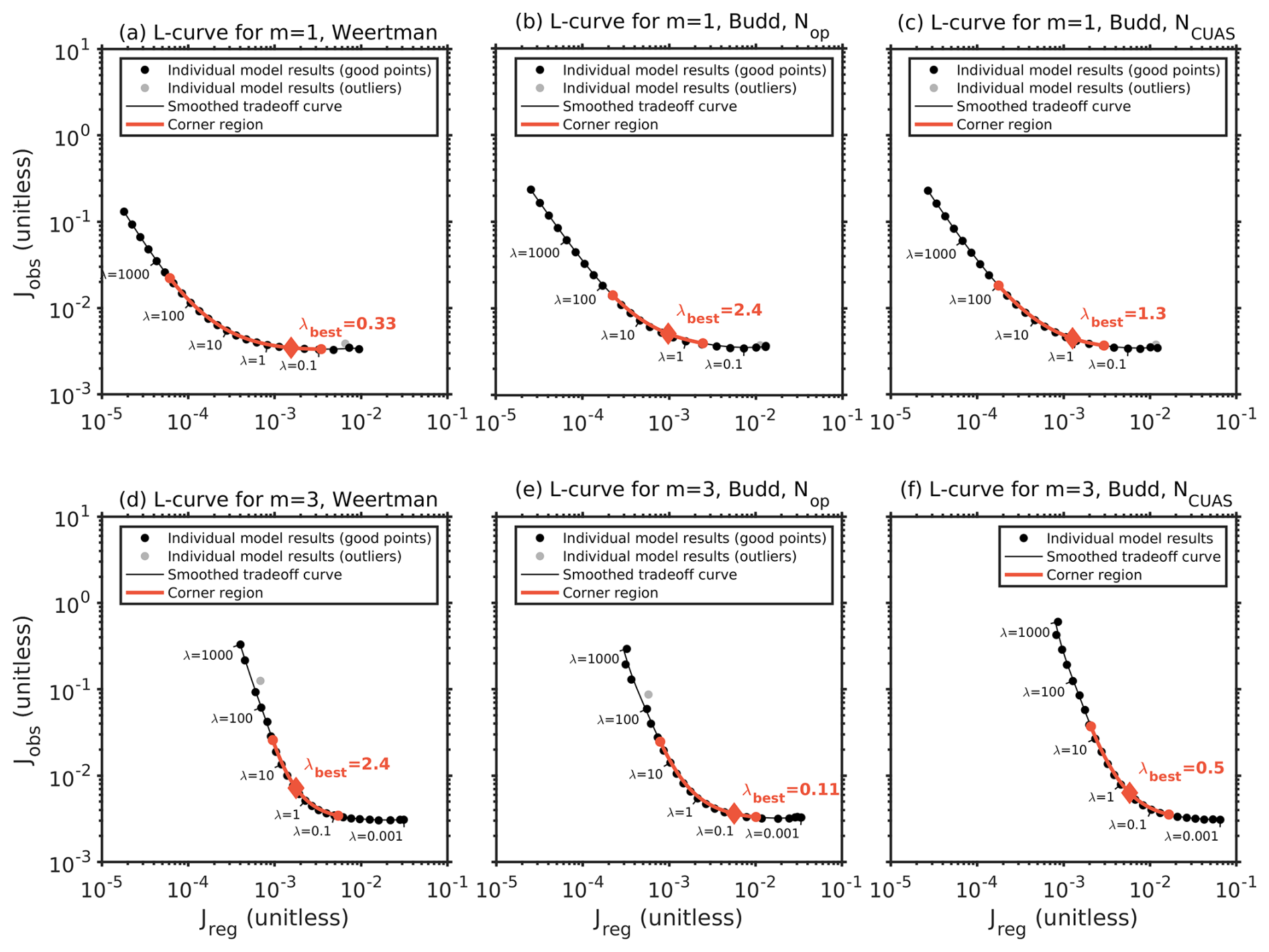
Figure 6 All six conducted L-curves in a log–log plot for the regularization cost J_reg against the data cost J_obs. The black dots indicate the inversion result for each λ value, the black line describes the smooth trade-off curve passing through the 25 different model samples, and the red area shows the corner region of the L-curves. The red points describe the λ_min and λ_max values, and the red diamond marks the λ_best value. Gray dots indicate outliers. (a) L-curve result for the linear Weertman friction law with λ_best=0.33. (b) L-curve for the linear Budd-type friction law including effective pressure from geometry N_op with λ_best=2.4. (c) L-curve result for the linear Budd-type friction law using the effective pressure from CUAS-MPI N_CUAS with λ_best=1.3. (d) L-curve for the nonlinear Weertman friction law with λ_best=2.4. (e) L-curve result including the linear Budd-type friction law for the effective pressure from geometry N_op with λ_best=0.11. (f) L-curve for the effective pressure N_CUAS with λ_best=0.5. Note that λ_best is a specific point determined by the maximum curvature and does not necessarily correspond to one of the λ samples.

We classify inversion runs as outlier models (gray dots in Fig. 6) if they fail to fully converge or if the cost function result exhibits non-monotonic behavior. In addition, we further declare models as outliers if they lie over a certain distance from the next data cost or regularization cost model by choosing a threshold value. All six L-curve runs exhibit few outliers with a maximum of one outlier per L-curve.

However, we observed difficulties in achieving convergence for λ values that are too small, especially when a linear friction law (m=1) is chosen for the inversion in a range of $\mathit{\lambda }\in \left[{\mathrm{10}}^{-\mathrm{3}},{\mathrm{10}}^{\mathrm{3}}\right]$. These outlier models probably arise because the regularization term is weighted too low and the misfit term is weighted too high at small λ values. Regularization is essential for transforming the ill-posed inverse problem, characterized by numerous local minima, into a more convex form, as convex functions have only a single global minimum (Rockafellar, 1970). This helps the optimization algorithm achieve an optimal solution. Insufficient regularization (small λ values) leaves the problem non-convex, increasing the likelihood of outlier models. However, in this case, one possibility is to avoid small λ values, which are unimportant from a mathematical perspective anyway, by shifting the λ range upwards to higher values. Therefore, the L-curves of our study are presented such that those with a linear friction law are shown for a range of $\mathit{\lambda }\in \left[{\mathrm{10}}^{-\mathrm{2}},{\mathrm{10}}^{\mathrm{4}}\right]$, while those with a nonlinear friction law are shown for a range of $\mathit{\lambda }\in \left[{\mathrm{10}}^{-\mathrm{3}},{\mathrm{10}}^{\mathrm{3}}\right]$. Additionally, an appropriate λ range is crucial to achieve L-curves with a well-defined corner region to select the λ_best value. For linear sliding laws, a range of $\mathit{\lambda }\in \left[{\mathrm{10}}^{-\mathrm{2}},{\mathrm{10}}^{\mathrm{4}}\right]$ avoids overly flat curves that make the corner region difficult to identify when the vertical limb is barely recognizable. Conversely, for nonlinear sliding laws (m=3), a range of $\mathit{\lambda }\in \left[{\mathrm{10}}^{-\mathrm{3}},{\mathrm{10}}^{\mathrm{3}}\right]$ ensures a clearer corner by extending the flat λ limb. In addition, the characteristic scale (Eq. 8) helps us to find a matching λ range that contains both limbs of the L-curve and thus guarantees a valid corner region.

Another approach to addressing the convergence issue involves using nearest-neighbor averaging to smooth the initial drag coefficient k_init resulting from the driving stress (see Eq. 6) for the runs with linear friction law. Unfortunately, further smoothing (3 times nearest-neighbor averaging) was needed for the runs with nonlinear friction to ensure the convergence of all those runs. This is likely because fine-scale structures in the initial basal drag coefficient k_init are too complex for the solver to handle. Since the convergence criterion depends on k_init (Eq. 9), such complexity can make it difficult to achieve a solution for stress balance.

In general, it helps to further adjust the convergence criteria ϵ_gttol and ${\mathrm{\Delta }}_{x_{\text{min}}}$ (Eq. 9) if the convergence of optimization is not achieved. For example, when an inversion only converges with ${\mathrm{\Delta }}_{x_{\text{min}}}$ during the line search, it is recommended to set ${\mathrm{\Delta }}_{x_{\text{min}}}$ more strictly. In our case, we achieved the best results with ${\mathit{ϵ}}_{\text{gttol}}={\mathrm{10}}^{-\mathrm{3}}$ and ${\mathrm{\Delta }}_{x_{\text{min}}}={\mathrm{10}}^{-\mathrm{5}}$ for inversion runs using a linear friction law. For convergence of the L-curve runs with a nonlinear friction law, we had to set the convergence criterion much more strictly to ${\mathit{ϵ}}_{\text{gttol}}={\mathrm{10}}^{-\mathrm{6}}$ and ${\mathrm{\Delta }}_{x_{\text{min}}}={\mathrm{10}}^{-\mathrm{4}}$. This was also observed in the study by Wolovick et al. (2023a) when nonlinear friction laws were used.

Overall, we were able to significantly reduce the outliers of the different L-curves and achieved convergence for most of the inversion runs. Admittedly, the mentioned adjustments slightly limit the comparability between simulations with linear and nonlinear friction laws. Further details on the convergence behavior of the inversion can be found in Appendix A.

3.2 Subdomain L-curve analysis

To explore how the optimal regularization of the inverse problem depends on glaciological settings or prominent subdomains, we analyze L-curves for selected subsets of our domain. For each subdomain, we compute the components of the cost function J_obs and J_reg, including only the model elements within the respective subdomain region. Since we do not recalculate the characteristic scaling factors (Eq. 8) for these subdomains or adjust for the fact that we are integrating over a smaller area, these subdomain L-curves are shifted towards smaller values relative to the full-domain L-curve. However, their relative shapes reflect the glaciological differences between these regions.

Here, the subdomain L-curve analysis is performed for a linear and a nonlinear Budd-type friction law experiment, both including N_CUAS. Figure 7a shows the eight different subdomains, aiming to include a wide variety of glaciological settings and prominent subdomains. We choose subdomains representing the main trunks of Pine Island Glacier (Fig. 7b) and Thwaites Glacier (Fig. 7c), upstream tributaries of Thwaites Glacier (Fig. 7d), a slow-flowing region around the WAIS divide (Fig. 7e), tributary glaciers of Whillans Ice Stream that cross the Transantarctic Mountains in the presence of many rock outcrops (Fig. 7f), the shear margin of Whillans Ice Stream (Fig. 7g), the fast-flowing trunks of the Bindschadler and MacAyeal ice streams (Fig. 7h), and a subdomain that includes Roosevelt Island (Fig. 7i).

Figure 7 Subdomain L-curve using the data cost J_obs (y axis) and regularization cost J_reg (x axis) from the experiments $m=\mathrm{1},N_{\text{CUAS}}$ and $m=\mathrm{3},N_{\text{CUAS}}$. Panel (a) shows the study area plot from Fig. 1 with the eight selected subdomains marked by the dashed black lines. The labels (b)–(i) of the different subdomains reflect the corresponding L-curves. Panels (b)–(i) display the eight L-curves associated with the subdomains in blue for the experiment $m=\mathrm{1},N_{\text{CUAS}}$ and in purple for the experiment $m=\mathrm{3},N_{\text{CUAS}}$. The non-filled circles indicate outlier models.

When assuming a linear friction law (Fig. 7, blue), the L-curves of the subdomains provide very smooth results and outliers are only detected for very small λ. In particular the subdomains in Fig. 7b, c, and f–h show a well-behaved L-curve with a good curvature. In contrast, when assuming a nonlinear friction law (Fig. 7, purple), we obtain the smoothest L-curve for the subdomain, including Pine Island Glacier (Fig. 7b). Furthermore, the subdomain including the rock outcrop region (Fig. 7f) and the subdomain covering Thwaites Glacier (Fig. 7c) reveal relatively smooth L-curves with a well-defined curvature. Overall, we get many outliers in the L-curves for larger λ using the nonlinear friction law, such as in the subdomains of the WAIS divide (Fig. 7e), in the area of shear margins from Whillans Ice Stream (Fig. 7g), in the upstream tributary of Thwaites Glacier (Fig. 7c), and in the L-curve of the MacAyeal and Bindschadler ice streams (Fig. 7h). This shows us that the smooth L-curve incorporating the entire model domain (Fig. 6f) suppresses those outliers for increased λ values. However, we found that nonlinear sliding produced numerous outliers in the L-curves at higher λ values, leading us to shift the λ range downward, as discussed in Sect. 3.1. The shift for λ could already lead to an improvement in the smoothness of the L-curve when integrating over the entire domain but not for the individual subdomains. This could also be explained by the fact that some of the subdomain L-curves are very smooth and have fewer outliers, and, if these predominate, the few outliers in other areas are suppressed during integration over the entire domain.

The subdomain covering Roosevelt Island generated quite a steep L-curve for both linear and nonlinear sliding, with only a slight hint of a corner at the lower end (e.g., Fig. 7i). This region might show a stronger corner if we extended the analysis to smaller λ values. However, observed velocities are very slow in this ice rise, and the apparent flattening at the low end may simply reflect the inability of the inverse model to reduce the misfit below the noise level of the observations. In that case, the straight-line (power-law) shape of the Roosevelt Island L-curve may reflect the fact that this ice rise is likely frozen to the bed (Martín et al., 2006) and is thus poorly suited to a basal sliding inversion. In contrast, we observe that the subdomain in the upstream tributary of Thwaites Glacier (Fig. 7d) and the subdomain in the WAIS divide (Fig. 7e) reveal a very flat L-curve. This suggests that subdomain L-curves characterized by lower velocities are not of major relevance for individual basal drag inversions, as J_obs remains in a similar order of magnitude for each regularization weight λ. This implies that not much regularization is required, as these regions may exhibit lower variability in the basal drag coefficient, especially when using linear sliding. It could be possible that a shift towards a higher λ range would show a proper curve. For m=3, this is not the case, as we have significantly more outliers in both regions for higher λ values. It is conspicuous that the subdomain covering many rock outcrops of the tributary glaciers of Whillans (Fig. 7f) shows relatively smooth behavior for m=1 and m=3. Since the modeling of rock outcrops is not straightforward, this gives us confidence in our treatment of modeling those areas. In particular, when those inversions lead to unexplainable issues, this analysis can be used to find errors that are not directly accessible or even to discover specific regions that could cause these problems. Overall, we can learn from this subdomain L-curve analysis how the L-curve behaves for regions with different glaciological settings or prominent subdomains. In general, Fig. 7 shows that different regions require different λ_best weights for regularization.

3.3 Effective pressure

To assess the influence of subglacial hydrology realizations on basal drag inversion results, we test both Weertman and Budd friction laws using effective pressure fields derived from geometry (N_op; Fig. 5a) and the CUAS-MPI hydrology model (N_CUAS; Fig. 5b). We analyze their impact on the six L-curves (Fig. 6) and the spatial distribution of basal drag emphasized with statistical values.

Figure 8a displays the three different L-curves that we obtain when using a nonlinear friction law (m=3). The turquoise L-curve with $N_{\text{CUAS}},m=\mathrm{3}$ shifts upwards to a higher $J_{\text{obs}}=\mathrm{71.84}\times {\mathrm{10}}^{-\mathrm{4}}$, compared to $J_{\text{obs}}=\mathrm{39.90}\times {\mathrm{10}}^{-\mathrm{4}}$ for m=3, N_op (Table 1). Overall, using N_CUAS in the nonlinear Budd friction law resulted in fewer convergence issues, as highlighted by the absence of outliers. In comparison, Fig. 9a shows the three L-curves for the linear friction law case. Here, the L-curve for N_op and the one for N_CUAS are almost identical in the linear case. This is emphasized by the same order of magnitude from $J_{\text{obs}}=\mathrm{46.96}\times {\mathrm{10}}^{-\mathrm{4}}$ for $m=\mathrm{1},N_{\text{CUAS}}$ and $J_{\text{obs}}=\mathrm{58.55}\times {\mathrm{10}}^{-\mathrm{4}}$ for $m=\mathrm{1},N_{\text{op}}$. The L-curve using a linear Weertman friction law shows a value of $J_{\text{obs}}=\mathrm{38.49}\times {\mathrm{10}}^{-\mathrm{4}}$ which fits with the slight downward shift in the L-curve (Fig. 9a). In total, we get the best performance of the L-curves regarding the J_obs and J_reg for using Weertman sliding regardless of using linear or nonlinear sliding (Fig. 8a, Fig. 9a). All J_obs values (Table 1, column 7) align with the λ_best values of the L-curves for the various experiments (Fig. 6), as higher λ_best values correspond to greater surface velocity mismatches and vice versa.

The λ_best value, determined by the maximum curvature in our curve-fitting procedure, generally coincides with the corner of most L-curves (visual perspective), except in Fig. 6a and e, where it would probably be visually selected with a slightly higher value. Looking at Figs. 8b–d and 9b–d representing the corresponding curvature of the total cost function (gray line) for Fig. 6a and e, a broad region of high curvature representing the visual corner with a narrow side peak (describing the maximum curvature) leads to selecting the latter as λ_best. This results in a slight deviation from the mean of the broader region and, consequently, from the visual corner.

Table 1 Table of statistical values for the grounded domain (Fig. 2f) of all six conducted experiments, each evaluated at its λ_best point. The reference experiment with the Weertman sliding is denoted by $k_{\text{W}}^{\mathrm{2}}$ and J_obs,W with m=1 and m=3, respectively, depending on which experiment is considered. We consider the variance σ² in the logarithmic squared basal drag coefficient ln(k²) and the logarithmic basal drag ln(τ_b), along with the variance ratio of both. The correlation R² of effective pressure N and basal drag coefficient k² regarding the reference experiment $k_{\text{W}}^{\mathrm{2}}$ is taken into account. The table displays the observational costs J_obs and the velocity equivalent of J_obs scaled by the velocity RMS. For the valuation of the whole model, we inspect the total model ratio with respect to the variance σ² in the ratio ln(k²) to ln($k_{\text{W}}^{\mathrm{2}}$) times the ratio of velocity misfit J_obs. Table 1 from Wolovick et al. (2023a) serves as a reference for this table.

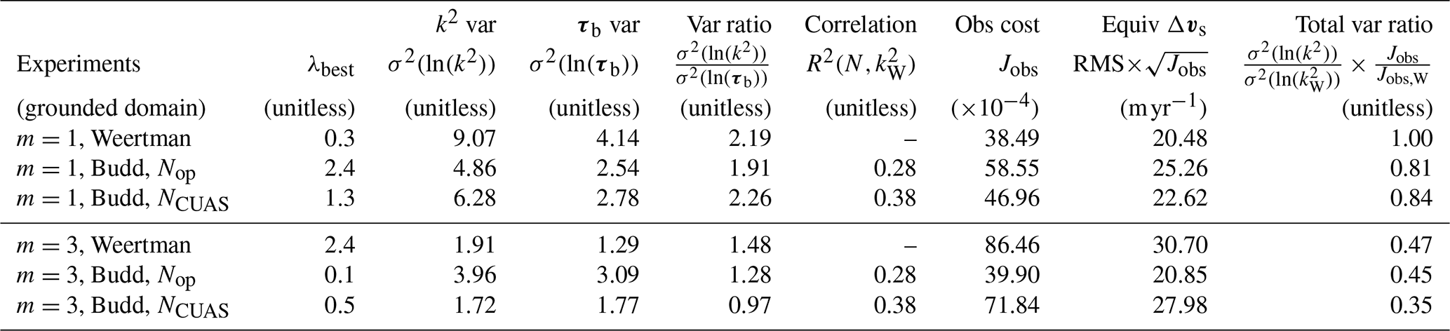
To compare the inferred basal drag based on Weertman- and Budd-type sliding, we refer to Eq. (3), assuming $k_{\text{W}}^{\mathrm{2}}=k_{\text{B}}^{\mathrm{2}}N$, to reproduce the same velocity and stress fields for both sliding laws, where $k_{\text{W}}^{\mathrm{2}}$ and $k_{\text{B}}^{\mathrm{2}}$ are the squared basal drag coefficients for Weertman and Budd sliding, respectively. A strong linear and positive correlation between N and $k_{\text{W}}^{\mathrm{2}}$ results in a smooth $k_{\text{B}}^{\mathrm{2}}$ field, as most variability is already captured by N, while a weak correlation requires more structure in $k_{\text{B}}^{\mathrm{2}}$ to fit observations. In an ideal scenario, N would entirely capture the spatial variation in $k_{\text{W}}^{\mathrm{2}}$, while $k_{\text{B}}^{\mathrm{2}}$ would remain constant within a specific region (subglacial substrate, geological formation) where no significant variations are expected on small length scales. Overall, while the sliding-law change should minimally impact the basal drag field, the inferred basal drag coefficients would differ significantly. A positive correlation between N and $k_{\text{W}}^{\mathrm{2}}$ ensures that the basal drag inversion introduces minimal structure into $k_{\text{B}}^{\mathrm{2}}$, as reflected in the positive R² values for N versus $k_{\text{W}}^{\mathrm{2}}$ shown in Table 1 (sixth column). In total, N_CUAS shows a slightly stronger positive correlation with $k_{\text{W}}^{\mathrm{2}}$ than N_op.

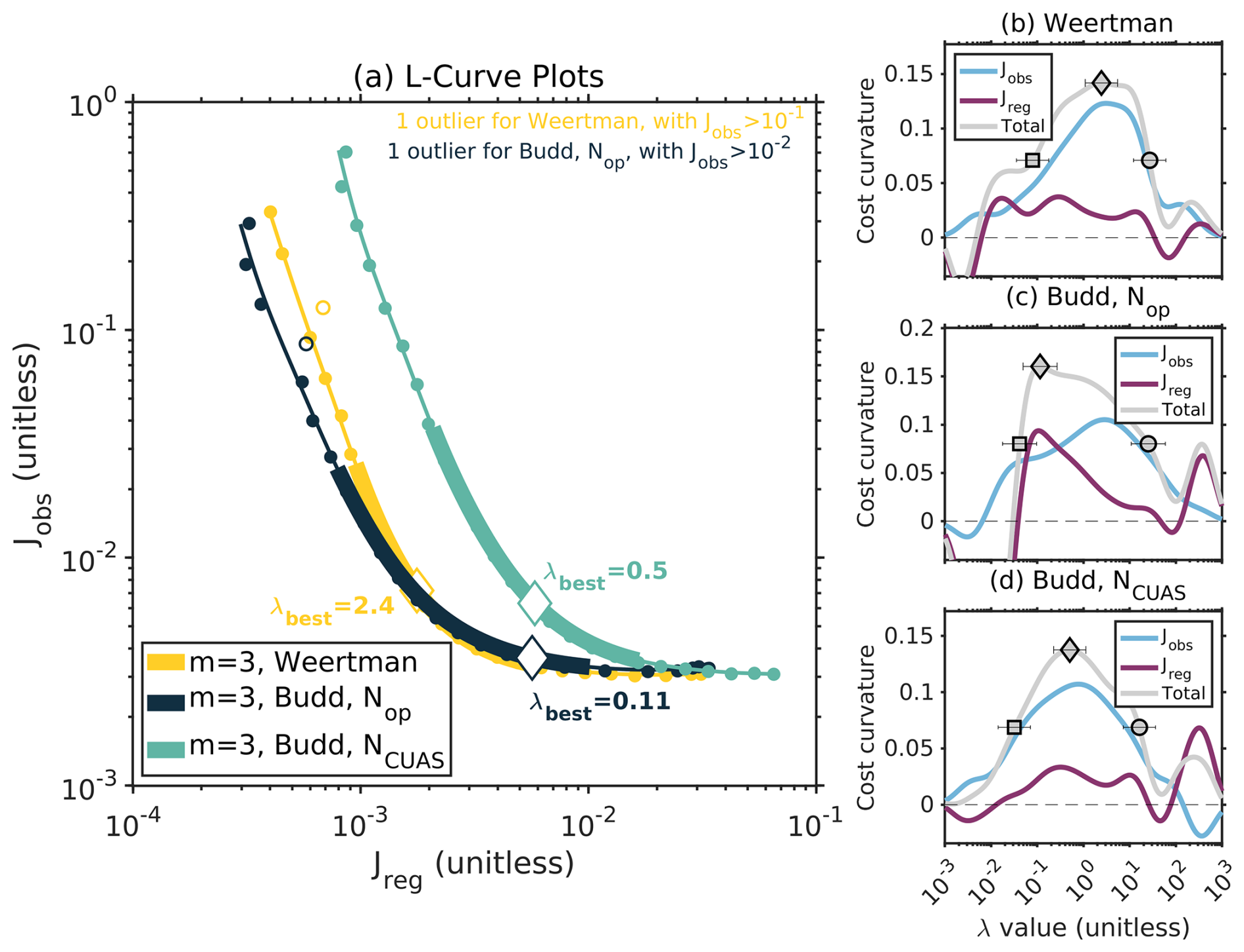
Figure 8 L-curves with nonlinear Weertman- and Budd-type friction laws. (a) The L-curve for nonlinear Weertman sliding is in yellow, and the L-curves for the nonlinear Budd friction law including N_op and N_CUAS are in dark blue and turquoise, respectively. The solid line represents the smooth trade-off curve, the thicker line characterizes the corner region, and the white diamond marks the λ_best value in each of these L-curves. One inversion run is detected as an outlier for Weertman sliding and Budd with N_op and is illustrated with the non-filled circles. Panels (b–d) display the cost curvature $\frac{d^{\mathrm{2}}\left(ln\right(J\left)\right)}{d\left(ln\right(\mathit{\lambda }){)}^{\mathrm{2}}}$ dependent on λ in the order for Weertman sliding (no N) and for Budd with N_op and N_CUAS, where the gray line represents the total cost function J, the purple line represents the regularization cost function term J_reg, and the blue line represents the velocity misfit cost function term J_obs in each of these three plots. The square marker displays the λ_min, the circle displays the λ_max, and the diamond displays the λ_best value.

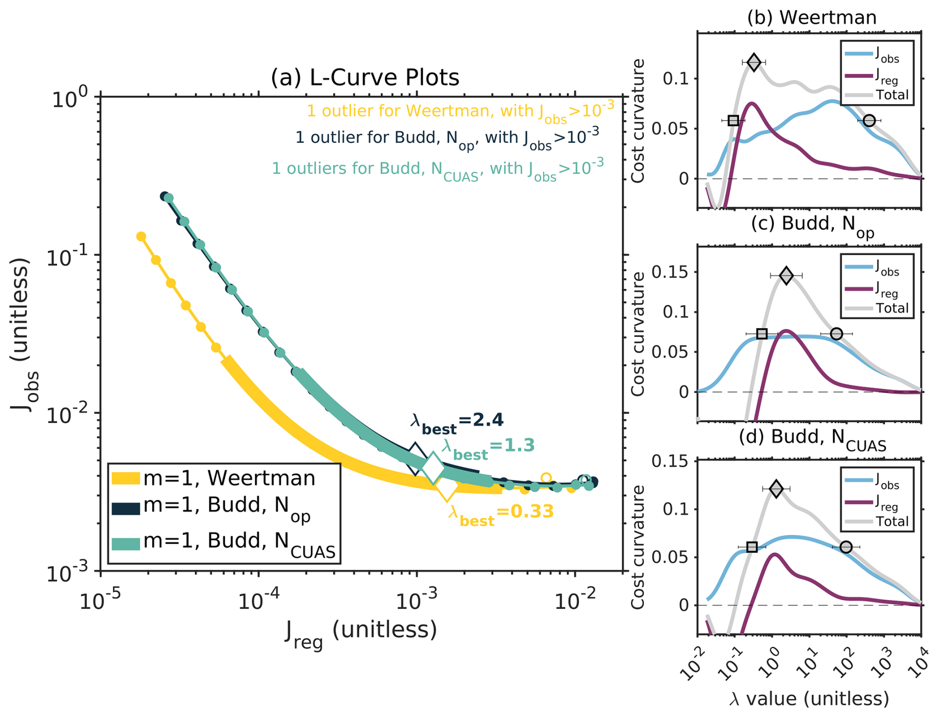
Figure 9 L-curves with linear Weertman- and Budd-type friction laws. The description is equivalent to the one in Fig. 8, only for the linear friction law instead of the nonlinear friction law. One inversion run is detected as an outlier (non-filled circles) for each of the three L-curves.

Figure 10 displays the resulting drag coefficient distribution k² for m=1 and m=3 with N_op and N_CUAS. To overcome the issue of non-comparability with respect to varying degrees of smoothness, when using different λ_best values, each basal drag coefficient is evaluated at the nearest (discrete) λ sample of the respective N_CUAS experiment. When comparing the structure of the basal drag coefficient shown in Fig. 10a and b and the distribution of the basal drag coefficient in Fig. 10c and d, we observe that, for all patterns, the N_op experiments exhibit more structure in k² than the experiments with N_CUAS. This finding is again emphasized by the correlation result $R^{\mathrm{2}}(N,k_{\text{W}}^{\mathrm{2}})$ in Table 1. Especially when we look more closely at Thwaites Glacier, a more ribbed structure can be identified, including N_op for both linear sliding m=1 and nonlinear sliding m=3. The intention is to use the subglacial hydrology model CUAS-MPI to obtain an effective pressure N_CUAS that captures most of the structure of the hydrology at the base, making k² smoother than with a Weertman friction law or with the often-used effective pressure from geometry, such as N_op. This would allow us to interpret the basal drag coefficient k² in terms of the physical properties of the subsurface rather than basal hydrology, since the hydrology is already included in the model. Overall, k² is 1 order of magnitude higher for N_CUAS compared to N_op for m=1 and m=3 (Fig. 10). This can be explained by the significantly higher magnitude of N_op in the whole study domain compared to N_CUAS (compare Fig. 5). This difference in magnitude is likely reflected in a higher basal drag coefficient k² for the N_CUAS experiments.

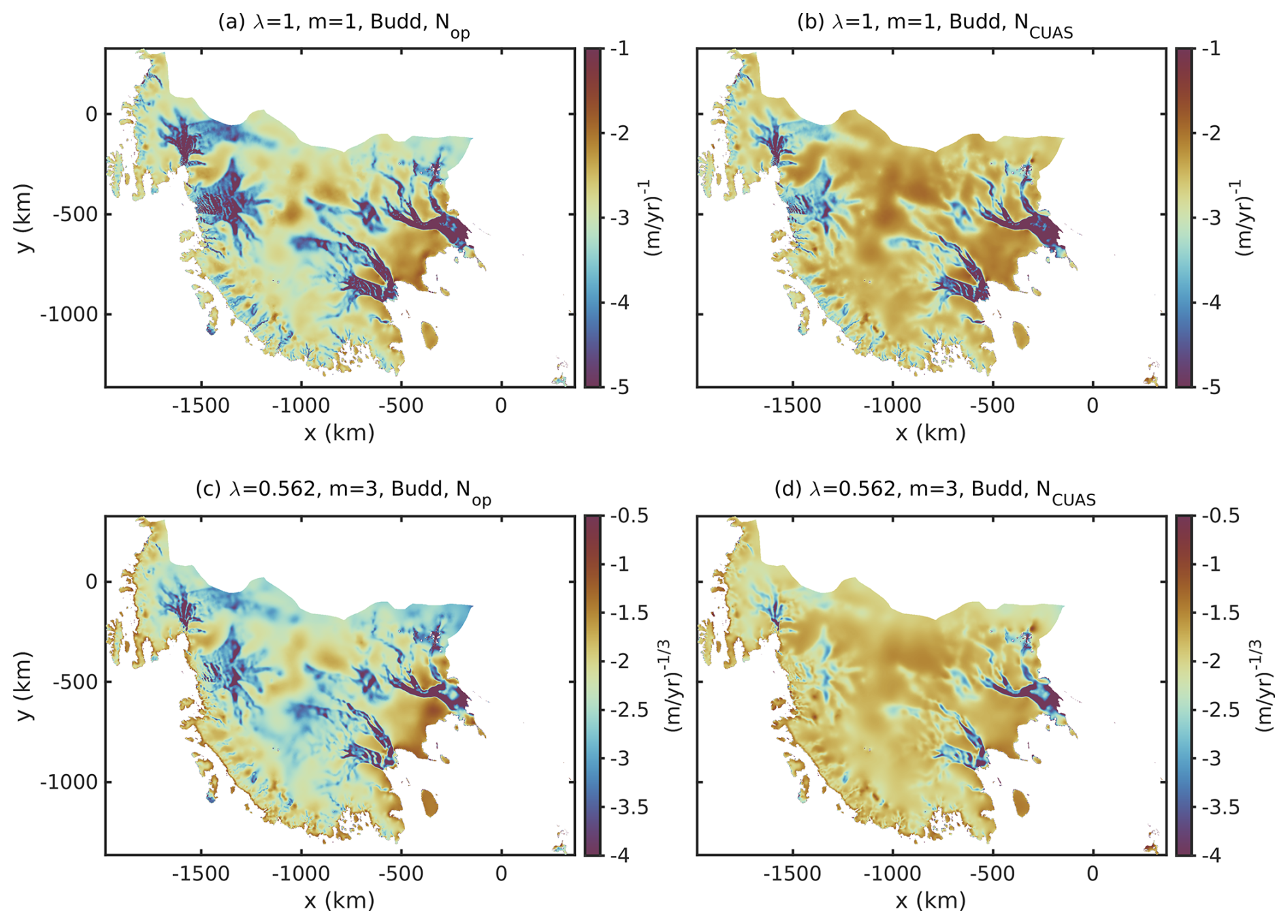
Figure 10 Drag coefficient maps of log10(k²) evaluated at the nearest (discrete) samples of λ_best of the L-curves. (a–b) The first row shows the drag coefficient of the inversion run, including a linear Budd friction law with m=1 and N_op (a) or N_CUAS (b). Both are evaluated at the λ_best≈1 of the L-curve using m=1 and N_CUAS for better comparison. (c–d) The second row describes the drag coefficient of the inversion run using a nonlinear Budd friction law with m=3 and N_op (c) or N_CUAS (d). Again, both are evaluated at the λ_best≈0.562 value of the m=3 and N_CUAS experiment for better comparison. Note the different units of the first and second rows.

We can evaluate the variance σ²(ln(k²)) (Table 1, column 3) to analyze a scale-independent measure of the structure generated by the basal drag inversion as described in Wolovick et al. (2023a). Incorporating effective pressure N_CUAS into the nonlinear sliding law results in the overall lowest variance value compared among the six experiments. An investigation of the total variance ratio of the basal drag inversion shows us the overall quality of the different experiments for the grounded domain (Table 1, column 9). Here, we observe a decrease whenever the effective pressure is included in the friction law.

3.4 Nonlinear versus linear sliding

In the following section, the effect of a linear versus nonlinear friction law on the L-curves is examined and emphasized with statistical values from Table 1.

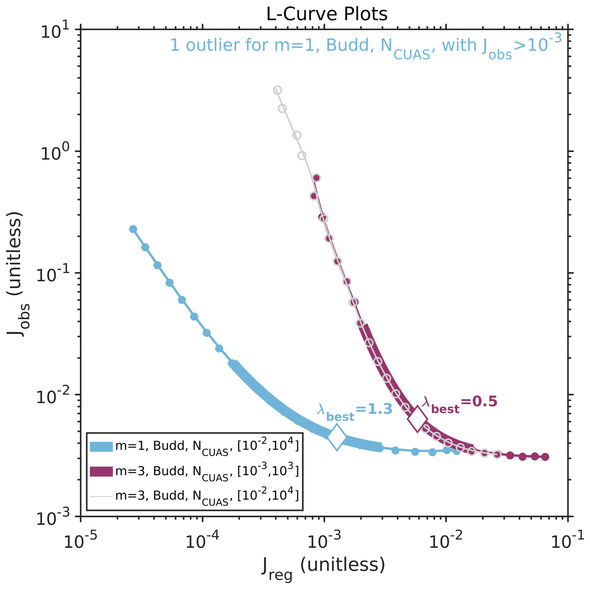
Figure 11 L-curve comparison plot for linear sliding m=1 and nonlinear sliding m=3 with N_CUAS. The blue curve illustrates the L-curve for linear sliding and N_CUAS with $\mathit{\lambda }\in [{\mathrm{10}}^{-\mathrm{2}},{\mathrm{10}}^{\mathrm{4}}]$. The purple curve illustrates the nonlinear friction law with N_CUAS and $\mathit{\lambda }\in [{\mathrm{10}}^{-\mathrm{3}},{\mathrm{10}}^{\mathrm{3}}]$. For a better comparison, the L-curve for the nonlinear friction law with N_CUAS in a range of $[{\mathrm{10}}^{-\mathrm{3}},{\mathrm{10}}^{\mathrm{3}}]$ is also given in gray. The dots explain the different inversion runs, the solid line indicates the smooth trade-off curve, the thicker line describes the corner region, and the white diamonds mark the λ_best for the L-curves shown. One inversion run for the L-curve with the linear friction law (m=1) including N_CUAS is detected as an outlier.

Figure 11 shows the L-curve for the linear Budd friction law $m=\mathrm{1},N_{\text{CUAS}}$ experiment (blue) alongside the nonlinear Budd-type friction law $m=\mathrm{3},N_{\text{CUAS}}$ experiment (purple). To get an impression of the different λ ranges used for linear and nonlinear sliding, we also show the L-curve of the $m=\mathrm{3},N_{\text{CUAS}}$ experiment in Fig. 11 with the shifted λ range $\left[{\mathrm{10}}^{-\mathrm{2}},{\mathrm{10}}^{\mathrm{4}}\right]$ (gray), which is also applied for the $m=\mathrm{1},N_{\text{CUAS}}$ experiment. The results in Fig. 11 show steeper L-curves for both cases of nonlinear sliding than for the L-curve results using the linear friction law. All four other experiments also exhibit this different shape behavior between linear (Fig. 6a–c) and nonlinear friction law (Fig. 6d–f). It can be recognized when comparing Fig. 8b–d to Fig. 9b–d that this could be explained by the increasing J_obs term and the more attenuated J_reg cost function term. Despite the choice of a different, upward-shifted λ interval, the L-curves with a linear friction law are still very flat in shape (Fig. 6a–c) compared to those of the nonlinear friction law (Fig. 6d–f). The corner region (e.g., Fig. 6) is defined by the range from λ_min to λ_max, which separates the flat and vertical limbs of the L-curve. The L-curves in the first row (Fig. 6, m=1, linear friction law) display a broader corner region, encompassing both lower and higher λ values compared to those in the second row (m=3). A narrower range between λ_min and λ_max simplifies the selection of an optimal λ, enhancing the reliability of the L-curves, which is evident in experiments with steeper nonlinearity.

When comparing the behavior of linear sliding (m=1) with nonlinear sliding (m=3), we recognize a decrease in variance in ln(k²) for both Weertman and Budd (Table 1, column 3). The decrease is especially high when considering Weertman and Budd sliding including N_CUAS. For m=1 using N_CUAS, we get velocity errors of $\sim \mathrm{23}\mathrm{m}{\mathrm{yr}}^{-\mathrm{1}}$, whereas we can determine an increase to $\sim \mathrm{28}\mathrm{m}{\mathrm{yr}}^{-\mathrm{1}}$ when considering a nonlinear friction law. However, overall, we recognize the strongest increase in velocity misfit of $\sim \mathrm{10}\mathrm{m}{\mathrm{yr}}^{-\mathrm{1}}$ when using a nonlinear Weertman friction law instead of a linear one. In total, only the velocity misfit of the friction law, including N_op, decreases when changing from linear to nonlinear sliding. This increase in velocity error is naturally linked to the decreasing weight of the regularization term λ_best (Table 1, column 2). Considering the variance ratio of ln(k²) and τ_b (Table 1, column 5), we get an overall decrease when using a nonlinear friction law. When comparing the total variance ratio of our basal drag inversion (Table 1, column 9), we get an improved performance for nonlinear sliding, independent of Weertman or Budd, reflected by a strong decrease in the total variance ratio.

If we compare the L-curves of the subdomains in Fig. 7 for experiment $m=\mathrm{3},N_{\text{CUAS}}$ to those of experiment $m=\mathrm{1},N_{\text{CUAS}}$, we can recognize that there are significantly fewer outliers for the linear sliding case, which only occur for very small λ, and the L-curves also appear smoother. In general, this result is consistent with the results we obtained for the six L-curve experiments we carried out for the entire domain (compare Fig. 6). It can be recognized that outliers in the linear L-curves (Fig. 6a–c) only occur for very small λ values, and the L-curves with the nonlinear sliding law (Fig. 6d–f) only show outliers for larger λ. The general shape in terms of steepness and flatness of the L-curves remains the same for nonlinear and linear sliding across all subdomains. However, as shown in Fig. 6, the domain L-curves including nonlinear sliding exhibit a steeper behavior. We conclude that linear sliding laws produce smooth subdomain L-curves with few outliers (Fig. 7), but different regions show varying λ_best values, indicating an influence of glaciological settings. However, when a nonlinear sliding law is applied, the impact of different glaciological factors appears to become more significant regarding the smoothness and outliers. We therefore suggest performing a subdomain L-curve analysis whenever a basal drag inversion for a larger model domain is considered, such as the WAIS.

3.5 Best drag estimate

In this section, we focus on the nonlinear Budd-type friction law experiment with N_CUAS, λ_best=0.5, as it represents the best estimate of basal drag τ_b and basal drag coefficient k² that we achieved (Fig. 6f). For this particular λ_best, the cost curvature (Fig. 8d) corresponding to the L-curve in Fig. 6f ($N_{\text{CUAS}},m=\mathrm{3}$) shows a clear peak at which our picking method selects the λ_best value. This would also be the position where the λ_best value would be chosen based on visual inspection of the L-curve. Although using λ_min yields a smaller velocity misfit (Fig. 14g versus Fig. 14h), this outcome is expected, as the L-curve method balances both cost function terms, making λ_best the optimal trade-off. Furthermore, we can emphasize our choice by showing in Sect. 3.3 that the inclusion of hydrology model results, such as N_CUAS in the Budd friction law, leads to a faster convergence (Fig. A1b) and to improvements in the resulting fields in terms of the reduction in the total variance ratio (Table 1, column 9) and the variance in k² (Table 1, column 3). Furthermore, we can point out in Sect. 3.4 that the use of nonlinear friction laws is advantageous, which is also reflected by the reduction in the total variance ratio of the derived basal drag parameter by half.

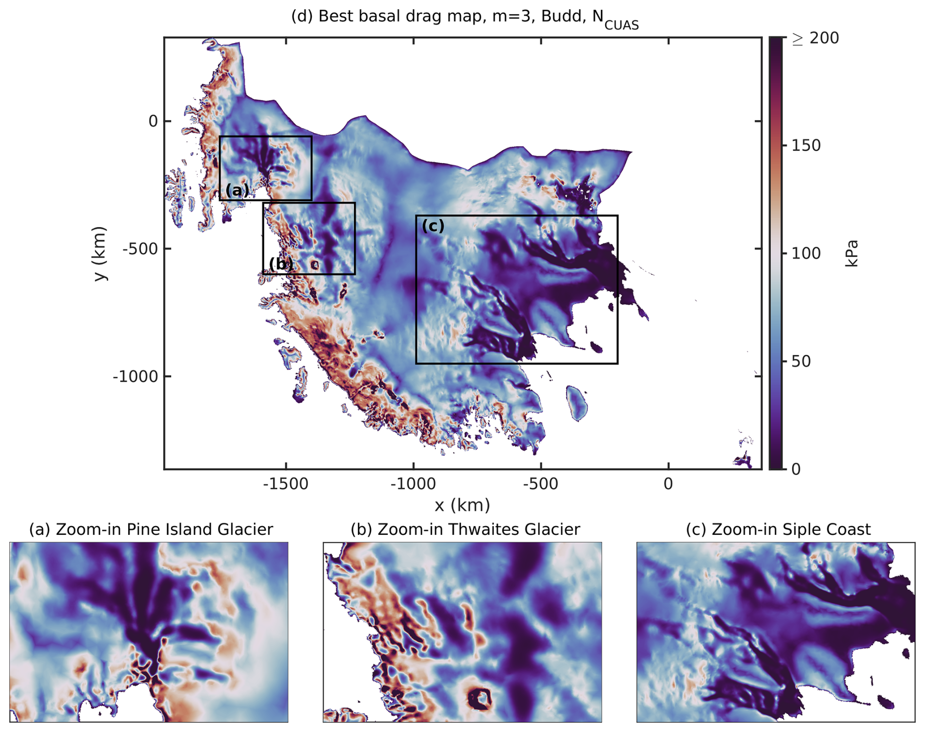
Figure 12 Map of the best-estimated basal drag result τ_b from WAIS inversion using λ_best=0.5 and nonlinear Budd sliding m=3 incorporating N_CUAS. The distribution is given (in kPa) within a range of [0,600]. Panels (a)–(c) display the zoom-in boxes for Pine Island Glacier, Thwaites Glacier, and the Siple Coast, as shown in Fig. 1.

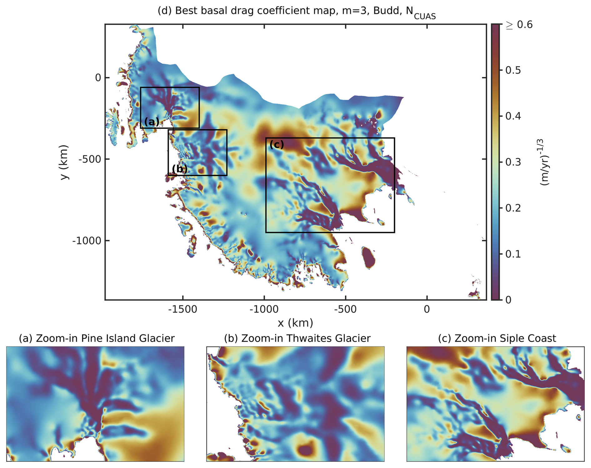
Figure 13 Map of the best-estimated basal drag coefficient result k² from WAIS inversion using λ_best=0.5 and nonlinear Budd sliding m=3 incorporating N_CUAS. The distribution is given within a range of [0,6] $(\mathrm{m}{\mathrm{yr}}^{-\mathrm{1}}{)}^{-\mathrm{1}/\mathrm{3}}$. Panels (a)–(c) display the zoom-in boxes for Pine Island Glacier, Thwaites Glacier, and the Siple Coast, as shown in Fig. 1.

Figure 12d shows the resulting spatial distribution of the basal drag τ_b. As expected, all glaciers with fast-flowing areas (Fig. 2e) are characterized by a relatively low basal drag (Fig. 12a–c). This can be recognized in Pine Island Glacier and at the Siple Coast (Mercer, Whillans, Bindschadler, and MacAyeal ice streams; compare Fig. 1). Pine Island Glacier and MacAyeal Ice Stream display a rippled structure (Fig. 12c). Thwaites Glacier is particularly prominent in this regard, as the structure of the basal drag alternates between high and low basal drag (Fig. 12b). This particular structure is recognizable in the basal drag coefficient in Fig. 13b and could be caused by the underlying bed topography, which reveals a bumpy terrain (Fig. 2a). Overall, Fig. 13d shows a low drag coefficient over the entire study area, apart from Kamb Ice Stream, Roosevelt Island, and regions further upstream where slow-flowing areas dominate. Kamb Ice Stream exhibits a very high drag, which is in line with the findings of Joughin and Tulaczyk (2002) and Beem et al. (2014), indicating that the glacier is frozen to its bed. In addition, Fig. 13 reveals that large parts of the domain, excluding the Siple Coast, exhibit high values of basal drag coefficient (red areas) near the grounding line, a pattern also reflected in the basal drag field (Fig. 12).

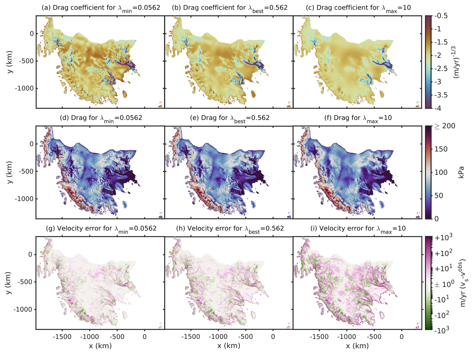
Figure 14 Map of the best drag coefficient, best drag estimate, and velocity error from left to right for the minimum acceptable λ_min, the λ_best, and the maximum acceptable λ_max of the experiment with nonlinear Budd-type sliding including N_CUAS. Panels (a)–(c) show the basal drag coefficient log10(k²) (in $(\mathrm{m}{\mathrm{yr}}^{-\mathrm{1}}{)}^{-\mathrm{1}/\mathrm{3}}$) within a range of $\left[-\mathrm{4},-\mathrm{0.5}\right]$. Panels (d)–(f) display plots for basal drag τ_b (in kPa) within a range of [0,600]. Panels (g)–(i) illustrate the velocity error on a symmetric logarithmic scale (in m yr⁻¹).

We conduct comparisons of λ_min, λ_max, and λ_best from the associated L-curve (Fig. 6f) for the basal drag coefficient k², the basal drag τ_b, and the velocity error ${\mathit{v}}_{\text{s}}-{\mathit{v}}_{\text{s}}^{\text{obs}}$ given by a symmetric logarithmic scale (Fig. 14). It should be noted that we do not use λ_best=0.5 to show the fields in Fig. 14 but instead use the nearest-neighbor λ sample of λ_best, λ_min, and λ_max from the resulting L-curve in Fig. 6f. When comparing our results for λ_min=0.0562, λ_best=0.562, and λ_max=10 in the first row of Fig. 14, we can observe the effect of the different weighting of regularization. The basal drag coefficient k² for λ_max displays a very smooth distribution with barely any structure. On the other hand, λ_min shows a patchy structure with possible artifacts. This occurrence can also be recognized in the same way in the basal drag τ_b (Fig. 14d–f). In addition, Fig. 14i has a rather high velocity error (${\mathit{v}}_{\text{s}}-{\mathit{v}}_{\text{s}}^{\text{obs}}$) widespread on the entire domain. However, this is not surprising, as λ_max=10 provides a high weighting for the regularization term J_reg, which is minimized together with the first velocity misfit cost term J_obs. Therefore, the velocity misfit can not become as small as in Fig. 14g. The striking feature here is the large velocity error at the edge of the whole domain in Fig. 14h and i. In general, the velocity misfit results in a patchy distribution of both overestimated surface velocities v_s, indicated by pink areas, and underestimated modeled surface velocities, indicated by green areas.

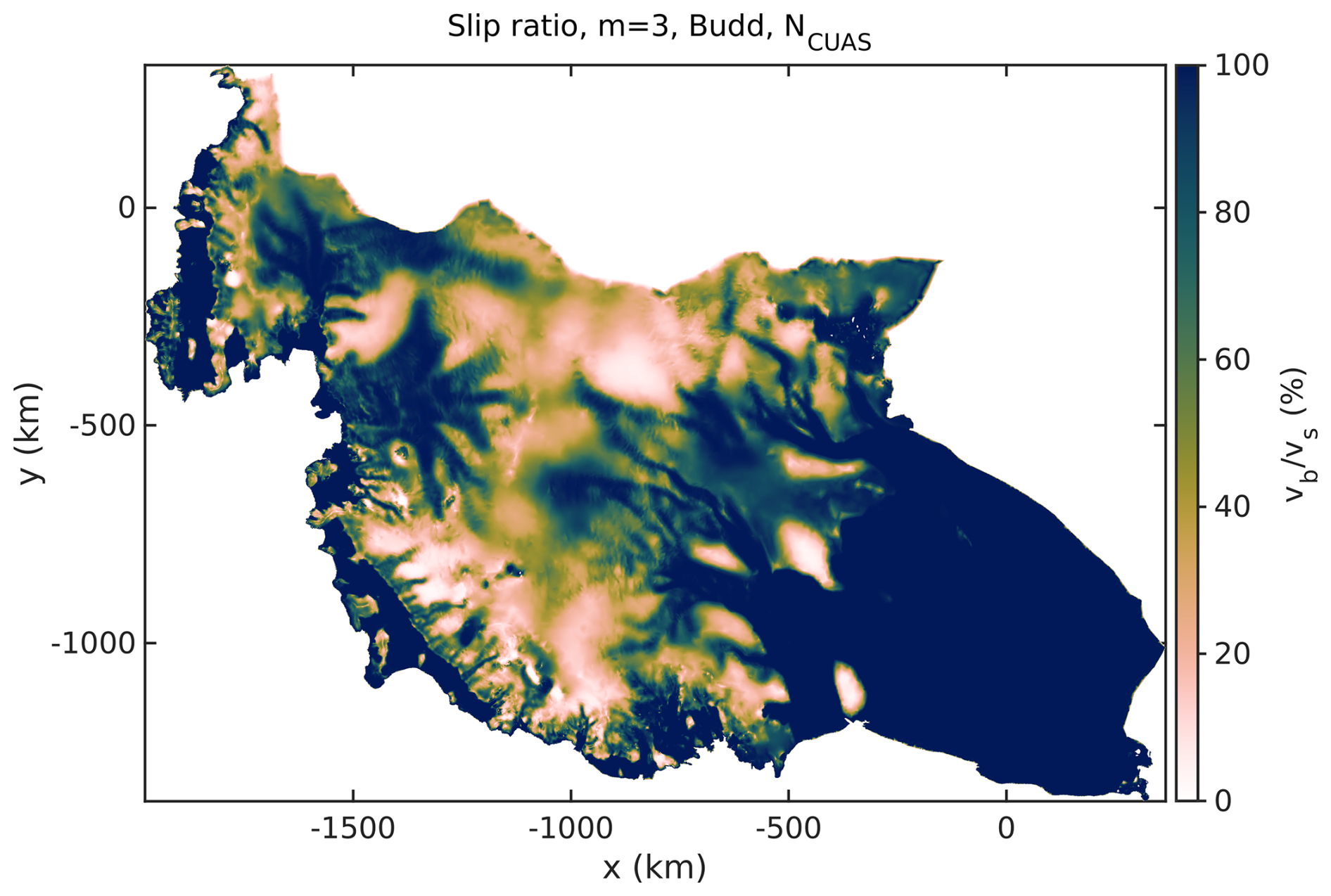
Figure 15 Map of the slip ratio between basal and surface velocity $v_{\text{b}}/v_{\text{s}}$ for the experiment with nonlinear Budd-type sliding including N_CUAS at λ_best=0.5.

Figure 15 displays the ratio of basal and surface velocity, which provides us with information on the creep-to-sliding behavior of the WAIS. The result shows that a high proportion of the velocity is caused due to sliding at the base (blue areas) exactly in those locations where high velocities (Fig. 1) and a low basal drag τ_b (Fig. 12d) predominate. When focusing on Thwaites Glacier again, a ribbed structure of velocities caused by alternating sliding and creep is visible. Another striking feature is the high percentage of creep in some locations of the Thwaites grounding line, which matches with the high basal drag (Fig. 12b). Assuming that Roosevelt Island is frozen to the bed, the high proportion of velocity represented by creep (red and white areas) seems to be very suitable at this location. The high percentage of creep in the area of Kamb Ice Stream also aligns with the expectation that Kamb is sticking to its bed.

4 Discussion

4.1 L-curves

We observe different problems in our L-curve procedure, e.g., many outliers for $\mathit{\lambda }<{\mathrm{10}}^{-\mathrm{2}}$ when using linear friction laws, and convergence problems for nonlinear sliding. Most problems could be solved by shifting the λ range towards higher values, further smoothing the initial drag coefficient k_init or by choosing different values for the convergence criteria ${\mathrm{\Delta }}_{x_{\text{min}}}$ and ϵ_gttol in Eq. (9). The smoothness of our L-curves serves as an indicator of whether the model and numerics are performing correctly, with many outliers suggesting issues in the setup or underlying assumptions. As already mentioned, the occurrence of outlier models at small λ values is probably related to the non-convexity of the inverse problem due to poor regularization, which makes it difficult for the optimization algorithm to find a global minimum. Overall, the results of the six experiments, which consistently show smooth L-curves with few or no outliers, give us confidence that our model procedure is trustworthy.

From a practical perspective, it would be preferable to select a single λ_best value for the whole of Antarctica. However, the results of our L-curve procedure and subdomain analysis reveal a range of λ_best values, making it challenging to select a single λ_best suitable for the entire domain. One way to overcome this issue is to apply a method as in Wolovick et al. (2023a), where different experiments are used to find the best overall drag distribution. Compared to the values for the λ_best values of the Filchner–Ronne region in Wolovick et al. (2023a), we obtain even higher λ_best values for the WAIS region. However, one should note here that our experiments are based on the higher-order equations (see Eq. 1) and that their inversion runs are based on the shelfy stream approximation (SSA equations). Simulating our region with the SSA equations (not shown in the paper) yields λ_best values of the same order of magnitude as described in Wolovick et al. (2023a). This fact would imply that an SSA inversion can resolve finer structures than an HO inversion.

Another approach for selecting optimal λ_best values could involve relying on a subdomain L-curve analysis, as demonstrated in Sect. 3.2. A key finding of this paper is that different regularization weights may be required for areas with fundamentally distinct physical conditions, leading to significant differences in ice flow. One potential method would be to determine λ_best values using an analysis setup similar to the control field approach (compare Fig. 3a, used for mesh generation with varying refinements). This could include a classification based on factors such as ice speed, surface and bed slopes, thickness gradients, or other notable physical differences. Overall, our subdomain L-curve analysis reveals that shear margin regions pose the greatest challenge when using nonlinear sliding laws. In contrast, slow-flow areas like the WAIS divide or upstream tributaries of Thwaites Glacier show minimal influence on regularization, regardless of linear or nonlinear sliding law. Similarly, rock outcrop regions affect the L-curve less than expected. Fast-flow regions such as Thwaites Glacier, Pine Island Glacier, and the Siple Coast exhibit relatively smooth subdomain L-curves for both linear and nonlinear sliding.

4.2 Utilizing hydrology models in inverse modeling

We discuss the influence of effective pressure and how our results differ for linear and nonlinear Budd and Weertman sliding. Like Wolovick et al. (2023a), we can argue that our results (Sect. 3.3) suggest that it is reasonable to use a nonlinear friction law for a basal drag inversion. Although our results show a strongly increased velocity equivalent for the misfit J_obs compared to Wolovick et al. (2023a), which even increases with nonlinear sliding, except for using N_op, we see an overall improvement when m=3 is used. This discrepancy from Wolovick et al. (2023a) could be justified by the higher-order equations used in our study or even due to our higher λ_best values. We observe a reduction by half of the total variance (Table 1, column 9) when switching from linear sliding m=1 to nonlinear sliding m=3. This gives us a measure of the overall performance of our inversion, whereby the increased velocity costs in J_obs are compensated by the reduction in the variance in ln(k²). Beyond that, the analysis of linear versus nonlinear sliding reveals flatter L-curves for m=1 and steeper ones for m=3. The steeper curves result in a narrower acceptable corner range for λ (Fig. 6), simplifying the determination of λ_best. These distinct curve behaviors between sliding laws are notable, with steeper L-curves for nonlinear sliding helping to precisely bracket the range from λ_min to λ_max, an observation also made by Wolovick et al. (2023a).

We agree with Wolovick et al. (2023a) regarding the nonlinearity of friction laws used in basal drag inversion, but our results concerning the use of effective pressure N differ somewhat. The location of the L-curve for the linear and nonlinear Weertman cases shows a slightly better performance than the L-curves for Budd sliding with N_CUAS (Fig. 8, Fig. 9). However, the velocity equivalent (Table 1, column 8) for nonlinear sliding is reduced from 30.70 m yr⁻¹ to 27.98 m yr⁻¹ when switching from Weertman to Budd including N_CUAS. On top of this result, we get the best performance using a nonlinear Budd friction law incorporating N_CUAS when looking at the total variance ratio (Table 1, column 9). McArthur et al. (2023) obtained a positive correlation between the effective pressure N and the basal drag coefficient k when using a Schoof sliding law but not when they referred to a Budd-type sliding law. This differs from our results, as we also obtain a positive correlation when using the Budd-type sliding law (compare Table 1, column 6). Regions with a lower effective pressure N_CUAS also exhibit a lower basal friction coefficient k, again demonstrating the controlling role of the hydrological system (compare Fig. 5b and Fig. 13). The slightly increased correlation of N_CUAS with $k_{\text{W}}^{\mathrm{2}}$ compared to N_op with $k_{\text{W}}^{\mathrm{2}}$ shows that N_CUAS does not need to produce too much structure when computing J_obs. This is further supported by our result in Fig. 10, which demonstrates that N_CUAS leads to a smoother distribution of the basal drag coefficient k², which is our goal when including N_CUAS from a subglacial hydrology model. This confirms that the nonlinear Budd friction law with N_CUAS performs well with our model setup. Equally, the results of McArthur et al. (2023) show a smoother basal drag coefficient when the effective pressure of a subglacial hydrology model is included. Such a smooth and only slightly variable basal drag coefficient is desirable because the effective pressure field N should account for the entire structure by including the subglacial hydrology (recall $k_{\text{W}}^{\mathrm{2}}=k_{\text{B}}^{\mathrm{2}}N$).

In addition, our experiments show that for nonlinear sliding using Weertman or Budd including N_CUAS, the convergence of the optimization process is achieved in significantly fewer iteration steps (Fig. A1). Overall, we have to admit that the convergence results could be specific to the particular ISSM inversion process with the chosen optimization algorithm of M1QN3. Even if we recognize that the M1QN3 algorithm achieves good convergence, there are certainly improved algorithms that might achieve better convergence. However, we cannot say whether other algorithms, e.g., an interior point algorithm (Byrd et al., 1999), as shown in Barnes et al. (2021), perform better without further comparisons.

The confidence in this experiment $m=\mathrm{3},N_{\text{CUAS}}$ is further supported by the experience of better convergence and the resulting smoother L-curves when including N_CUAS. These key findings justify our argumentation in Sect. 3.5 to define the basal drag τ_b and the drag coefficient k² as our best estimate when using the experiment for $N_{\text{CUAS}},m=\mathrm{3}$. In general, our study, along with that of McArthur et al. (2023), demonstrates a more realistic representation of the ice sheet model when using the output of subglacial hydrology models, revealing the importance of coupling ice sheet models with subglacial hydrology models.

Joughin et al. (2019) recommend using a Coulomb friction law, which accounts for cavitation effects on sliding (Schoof, 2005), as it improved simulation fidelity, especially for Pine Island Glacier. Notably, Joughin et al. (2019, Fig. 1) illustrate that nonlinear power laws, such as m=3 used in our study, approximate the regularized Coulomb friction law for m>1. Consistent with our results and those of Wolovick et al. (2023a), nonlinear sliding laws improve model performance. However, incorporating subglacial hydrology provides better insights into basal water pressure, and a regularized Coulomb law, which is nonlinear concerning effective pressure, could further enhance the dependency of basal motion on hydraulic conditions. Therefore, adopting the Coulomb friction law from Joughin et al. (2019), which accommodates both weak till and hard bedrock, together with the effective pressure of the CUAS-MPI hydrology model, could improve accuracy in future studies.

4.3 Comparison with previous studies/findings in the WAIS

In this section, we compare our best drag and our best drag coefficient with findings of previous studies. When analyzing our best estimate of the basal drag τ_b and the basal drag coefficient k², we find high variability in the Thwaites region (Fig. 12b, Fig. 13b) and predominantly high velocities (Fig. 2e). Here, we observe characteristic rib-like patterns, so-called traction ribs (Sergienko and Hindmarsh, 2013), which vary between high basal drag τ_b around 200 kPa and very low regions of drag close to 0 kPa. Rib-like features are also observed in paleo-ice streams (Stokes et al., 2016). Stokes et al. (2016) suggest that the ribbed bedforms found under the ice masses could be caused by a topographic expression. Comparing our results with existing seismic measurements of the glacier bed reflection in the Thwaites region could provide us with further insights in the future. However, when we examine the Siple Coast for our best maps of basal drag (Fig. 12c) and basal drag coefficient (Fig. 13c), we have low variability, especially for the Mercer, Van der Veen, and Whillans ice streams. Nevertheless, when applying SSA instead of the HO equations, it would be possible to find a higher variability in this region due to the lower λ_best values we obtain when using SSA. In that case, the structure might not be smoothed as much as we observe here at higher λ_best values. Pine Island Glacier in Figs. 12a and 13a is represented by a relatively low basal drag and basal drag coefficient compared to the drag obtained from Morlighem et al. (2010). While our drag is quite equally distributed, the basal drag for Pine Island Glacier in Morlighem et al. (2010) shows a very patchy structure, but this could also be caused by the higher mesh resolution used in the study. Figures 12a and 13a highlight regions of increased basal drag and drag coefficient near the grounding line in large parts of the study area, except the Siple Coast. A similar pattern, with high drag concentrated along the margins, was identified by Höyns et al. (2024) and extends to the East Antarctic Ice Sheet and parts of the WAIS. This increased basal drag near the grounding line may play a crucial role in delaying future ice sheet retreat.

Morlighem et al. (2021) highlight that even small variations in basal friction significantly impact glacier dynamics when using automatic differentiation. In addition, Barnes and Gudmundsson (2022) show that simulations with lower basal friction coefficients exhibit greater sensitivity to changes in forcing. Although their study employs a constant basal drag coefficient to explore this effect, accurately characterizing the sliding laws and the basal drag coefficient remains crucial for reliable predictions of future ice sheet evolution. Our Fig. 14 illustrates how varying λ values influence the simulated basal drag fields, again demonstrating the importance of precise regularization values and the application of a subdomain L-curve analysis in the future.

Rathmann and Lilien (2022) assume that sticky spots are difficult to detect and that bed bumps could be misinterpreted when deriving the basal drag coefficient using Glen's flow law (Eq. 2). Indeed, some sticky spots identified in the literature, e.g., the sticky spot of Kamb Ice Stream (Luthra et al., 2017), are not visible in our resulting basal drag coefficient field (Fig. 13c) or in the basal drag field (Fig. 12c). We hypothesize that this could be due to the neglect of crystal-orientation fabric when inferring the basal drag coefficient k. However, the sticky spot could also be obscured by the regularization process; the lower mesh resolution in this region (Fig. 3b); or, in general, the fact that we consider a Budd-type sliding law incorporating an effective pressure field instead of using only Weertman sliding like Rathmann and Lilien (2022). In the latter case, the sticky spot could already occur in the effective pressure field, which is not recognizable in our case (compare Fig. 5).

Overall, we cannot argue if our basal drag coefficient would significantly change when considering anisotropic ice instead of isotropic ice as with Glen's flow law. In addition, the choice of flow law, e.g., using an anisotropic flow law or including an enhancement factor instead of using Glen's flow law (Eq. 2), could also further impact our results regarding the deformation-to-sliding ratio (Fig. 15). Considering our map in Fig. 15, it becomes apparent that most of the glaciers and ice streams in our study domain are controlled by sliding-dominated flow. Comparing these results with those of McCormack et al. (2022), who show that experiments with ESTAR (Empirical Scalar Tertiary Anisotropy Regime) and Glen using the enhancement factor E=5 (experiment G₅) reveal an increase in deformation-induced flow, especially in the defined deformation–sliding zone and the bed-parallel shear deformation zone, our results could change if the ESTAR flow law or at least an enhancement factor is included in Glen’s flow law.

According to Kyrke-Smith et al. (2018), our inferred basal drag conditions should be interpreted with caution, as they recommend separating skin and form drag. When performing the inversion with detailed bed topography data, they observed a reduced skin drag, indicating that the results could include drag, which is due to unresolved topography rather than inherent bed and sediment conditions. Uncertainties in the basal topography could contribute to errors in the inferred basal drag. In addition, Kyrke-Smith et al. (2018) suggest basing the inversion in areas where traction ribs can be found, such as in the Thwaites region, on high-resolution topography data, which was not implemented in this study. However, Schroeder et al. (2013) investigated the transition of the water system beneath Thwaites Glacier based on geophysical analysis. They found concentrated channels (no effect on basal drag) near the grounding line, followed by a transition to distributed channels (reducing basal drag) further upstream. Comparison of our basal drag distribution with these findings agrees well (Fig. 12b), as we observe a distribution of low drag further upstream that transitions into a distribution of higher drag near the grounding line.

The inversion method and the L-curve analysis presented could, of course, be extended to other iterative schemes, as demonstrated in Zhao et al. (2018), or to flow-rate-factor inversions (e.g., Arthern et al., 2015; Ranganathan et al., 2021; McArthur et al., 2023). Various studies suggest performing a combined inversion of basal drag and flow-rate factor; e.g., Rathmann and Lilien (2022) recommend such joint inversion to reduce mass-flux errors by compensating for missing fabric information when using Glen's flow law. Simultaneous determination of the flow-rate parameter and the basal drag coefficient would be necessary, as the ice velocity is controlled by both. When performing a single inversion, such as our basal drag inversion, we have to assume erroneous rheology and thus insert uncertainties into the resulting basal conditions (Ranganathan et al., 2021). However, we argue that both an iterative scheme and joint inversion need a good temperature–depth profile to get a good initial state after inversion, e.g., what Zhao et al. (2018) aim for, or to get a good joint inversion result. This is the reason why we restrict our inversion to an absolute misfit term in the cost function J. Inclusion of the logarithmic misfit term (e.g., Morlighem et al., 2013) would perform better if a rheology inversion were considered. The observed surface velocities in the interior of the study area are relatively slow, and, without proper choice of the rheology (temperature), the velocity contribution from ice deformation could already lead to a higher surface velocity than observed. In this case, the basal drag inversion could not correct for this bias, and the logarithmic misfit in these regions would likely be very high. Overall, changing the misfit term does not change the presented approach for the inversion of the basal drag with the used L-curve analysis. However, incorporating more knowledge into the calculation of rheology, such as a better temperature–depth distribution, could help in the future to obtain better results. Nevertheless, our aim was not to achieve the best steady state, e.g., as in Zhao et al. (2018). Our statement is that focusing on a smooth L-curve result in an inversion is also of great importance, as we experienced that any ill-formed L-curve was always due to difficulties in the inversion process, caused either by the input data or the numerics involved. For example, if the λ value is not selected in the corner of the L, whether due to an incorrect representation, e.g., not based on a log–log scale, or due to a subjective choice of the λ value, we would produce unrealistic artifacts in the basal conditions.

5 Conclusions

In this paper, we analyzed a total of six basal drag inversion experiments for a large part of the WAIS using both linear and nonlinear Weertman- and Budd-type friction laws with two different effective pressure descriptions. We particularly focused on a basal drag inversion using a Budd-type friction law incorporating an effective pressure from a hydrology model to improve the basal drag field for a major part of the WAIS. We developed a strategy to handle poorly shaped L-curves when weighting the regularization term and achieved six well-defined, smooth curves. We find that ill-shaped L-curves with many outliers are most likely the result of inconsistencies in the model setup that should be addressed. In all cases, we were able to achieve a smoother L-shaped curve if different actions, e.g., shifting the λ range, took place. The subdomain L-curve analysis reveals that subdomains with different geometry settings have an effect on the shape and smoothness of the L-curves. We can identify problematic areas in the study area through outliers in the L-curves of specific subdomains. Overall, this paper highlights the need for varying regularization values for different physical or geometric settings, leading to significant differences in ice flow and more accurate basal drag results.

Our results suggest, as in previous studies, that it might be useful to rely on a nonlinear friction law when using basal drag inversions. We demonstrate that, by including effective pressure from the subglacial hydrology model, CUAS-MPI can further improve the resulting maps of a basal drag inversion. We were able to show that the incorporated effective pressure field explains a significant fraction of the variance in the drag coefficient. However, we believe that we could achieve even better results for the basal drag coefficient by further improving the effective pressure of CUAS-MPI. The ribbed structure that we recognize in parts of Thwaites in our resulting basal drag and basal drag coefficient distributions could be confirmed in the future with seismic measurements. As we have high confidence in our results, our achieved basal drag can serve as an initial stress state for further models considering a major part of the WAIS. In the future, the behavior of the L-curves and their analysis should also be compared with the other areas of Antarctica or even the entire Antarctic.

Appendix A: Convergence of inversion

Figure A1 shows the convergence of the total cost function J for all six experiments of the optimization based on the λ_best weight (labeled in Fig. 6). The x axis displays the number of iterations required for the cost function J to reach an optimum. In the case of a linear friction law (Fig. A1a), 200 iterations are required on average. However, if a nonlinear friction law is used (Fig. A1b), fewer iteration steps of around 120 are required until convergence is reached. It is remarkable that the run with a nonlinear Budd friction law employing N_op requires up to 60 iterations more than the other two runs using a nonlinear friction law. In the case of the linear friction law (Fig. A1a), the inversion using a Weertman friction law requires significantly more iterations (about 70) for convergence than the two with the Budd-type friction law. In both the linear and nonlinear cases, the inversions involving a Budd friction law with the effective pressure N_CUAS require the fewest iterations until convergence is reached.

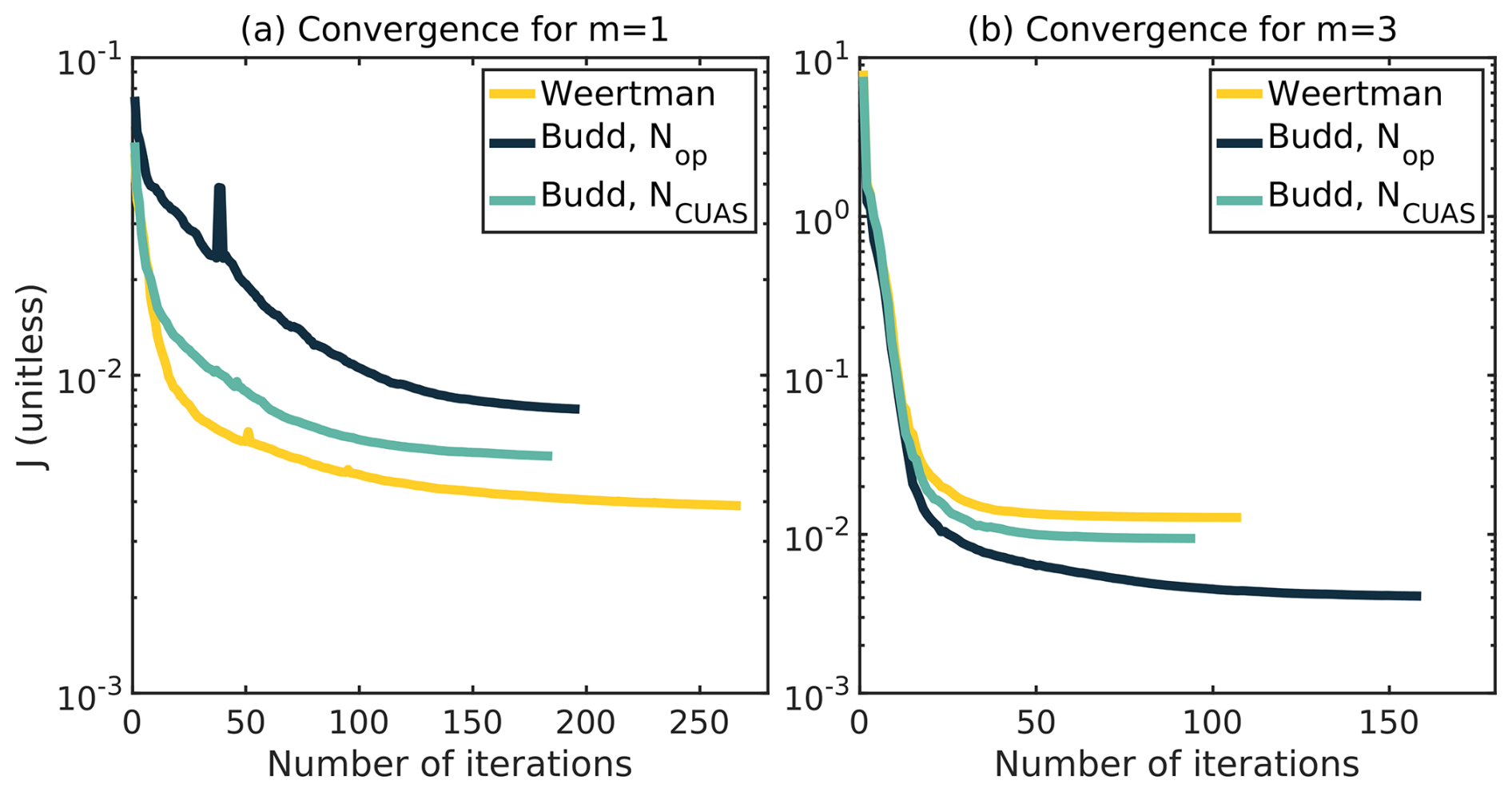
Figure A1 Convergence of cost function J for the respective best weight λ_bst of all six optimization runs. Note the different ranges of iteration steps for the x axis. (a) Convergence for the three experiments using a linear friction law. (b) Convergence for the three experiments with a nonlinear friction law. The yellow line indicates the convergence of the inversion using a Weertman friction law; the dark-blue line denotes the convergence of the inversion run with Budd-type and N_op; and the turquoise line characterizes the convergence of the run with Budd-type using N_CUAS, respectively, for panel (a) and panel (b).