Viscoelastic mechanics of tidally induced lake drainage in the grounding zone

Drainage of supraglacial lakes to the ice-sheet bed can occur when a hydrofracture propagates downward, driven by the weight of the water in the lake. For supraglacial lakes in the grounding zones of Antarctic glaciers, drainage mechanics are complicated by the glaciers' proximity to the grounding line. Recently, a series of supraglacial lake drainage events through hydrofractures were observed in the Amery Ice Shelf grounding zone, East Antarctica. The lake depth at drainage varied considerably between events, raising questions about the mechanisms that induce hydrofractures even at low lake depth. Here, we use a modelling approach to investigate the contribution of tidally driven flexure to hydrofracture propagation in the grounding zone. We model the viscoelastic response of a laterally unconfined marine ice sheet to tides, the tidally induced stress, and the contribution of this stress to hydrofracture propagation. A sensitivity analysis is used to explore the dependence of viscoelastic grounding-line dynamics on the material properties of ice and local bedrock bathymetry. We propose a model-based criterion that predicts hydrofracture and supraglacial lake drainage as a function of daily maximum tidal amplitude and pre-drainage lake depth in laterally unconfined grounding zones. Although lateral confinement may contribute to the dynamics of lake drainage at Amery, our model predictions are consistent with observations of hydrofracture events from this grounding zone.

1 Introduction

Atmospheric warming is driving increasing meltwater production on ice-sheet and ice-shelf surfaces (Trusel et al., 2015). In the melt season, this meltwater ponds in topographic lows and forms supraglacial lakes. Lakes drain either slowly, through surface drainage channels (Banwell et al., 2019), or rapidly, through hydrofractures (Das et al., 2008). Lake drainage through hydrofractures can impact the ice-sheet mass balance in various ways. In grounded ice sheets, hydrofractures efficiently transport surface meltwater to the subglacial hydrological system. This process reduces bed friction and thus modulates ice-flow velocity and flux (Das et al., 2008; Doyle et al., 2013; Tedesco et al., 2013; Stevens et al., 2015; Dunmire et al., 2020). At ice shelves, hydrofractures can initiate or promote rifts. When propagating through ice shelves, rifts can destabilise them by triggering iceberg calving and ice-shelf collapse (Scambos et al., 2000; Glasser and Scambos, 2008; Banwell et al., 2013, 2019; Warner et al., 2021; Lipovsky, 2020), which can lead to a loss of buttressing and increased ice-sheet mass loss.

In East Antarctica, satellite imagery suggests that supraglacial lakes often cluster in the grounding zone, particularly at low elevations and bed slopes. Many of these lakes are connected to surface drainage systems or are located in regions vulnerable to hydrofracturing (Stokes et al., 2019). In the grounding zone, besides lake-water pressure, tensile stress due to tidal flexure can promote hydrofracturing. Advection of the damaged ice produced in the grounding zone could destabilise the downstream ice shelf (Borstad et al., 2012). Thus, it is important to understand how hydrofractures are initiated and promoted in the grounding zone.

Trusel et al. (2022) reported a series of repeated drainage events at a supraglacial lake at the grounding line (GL) of the Amery Ice Shelf, East Antarctica. Interestingly, these drainage events did not occur at a threshold in lake volume; rather, they tended to coincide with times of high daily tidal amplitude. These observations raise the question: how do tides near the GL contribute to the ice-sheet stress field and lake drainage through hydrofracturing? Trusel et al. (2022) hypothesise that near the GL of the Amery Ice Shelf, drainage events are promoted by tensile stress due to tidal flexure. A close examination of remotely sensed data (Sect. 4) indicates that the lake studied by Trusel et al. (2022) is in the grounding zone of a laterally confined outlet glacier close to the shear margin of the Amery Ice Shelf. While data analysis by Trusel et al. (2022) shows that the lake drainages correlated with ocean tides, the dynamics at this locale may be complicated by the lateral shear of the upstream outlet glacier (Raymond, 1996; van der Veen and Whillans, 1996) and the lateral confinement of ice flexure (Antropova et al., 2024; Rignot et al., 2024). To present a simpler, more general treatment, we derive a model of tidal–GL migration and the associated hydrofracturing of a laterally unconfined marine ice sheet. This approach enables a detailed study of viscoelastic, tidal–GL dynamics and their sensitivity to ice material properties and local bed geometry.

The GL is the internal boundary between the grounded ice sheet and the floating ice shelf. Variations in its position affect the ice flux from inland to the sea. In Antarctica, the GL response to diurnal ocean tides has been documented by various observations. In the Rutford Ice Stream, West Antarctica, ice flow is modulated by semi-diurnal tides, with the tidal effects on the ice-flow rate propagating tens of kilometres upstream (Gudmundsson, 2006; Murray et al., 2007; Minchew et al., 2017). At the Amery Ice Shelf, kilometre-scale tidal–GL migration with seawater intrusion has been observed using differential radar interferometry (Chen et al., 2023). The observed grounding zone is much larger than predicted by hydrostatic equilibrium, raising questions about whether the observed tidal flexure within the grounding zone is associated with stresses that contribute to hydrofracturing.

Ice-shelf flexure at the GL can be modelled using thin-plate theory with an elastic (Vaughan, 1995; Sayag and Worster, 2011; Wagner et al., 2016; Warburton et al., 2020) or a viscoelastic constitutive relationship (Reeh et al., 2003; Gudmundsson, 2007). In these models, the GL is treated as a peeling front or the clamped end of the ice shelf. Thin-plate models capture the large-scale flexure of ice shelves and neglect the membrane stress that is associated with lateral extension. Moreover, various studies have used a vertically integrated theory with viscous constitutive law to investigate the dependence of steady-state GL position on ice thickness, sliding laws, buttressing effects, and bed topography (Schoof, 2007a, b, 2012; Katz and Worster, 2010; Tsai et al., 2015; Pegler, 2018; Haseloff and Sergienko, 2022; Sergienko and Haseloff, 2023). Besides depth-integrated models, full-Stokes models have also been used to study the migration of GLs on both longer timescales (Nowicki and Wingham, 2008; Durand et al., 2009; Favier et al., 2012; Gudmundsson et al., 2012; Cheng et al., 2020) and tidal timescales (Gudmundsson, 2011; Rosier et al., 2014, 2015; Rosier and Gudmundsson, 2020). In these models, the ice-sheet-bed contact problem has been incorporated as a boundary condition. More recent studies by Stubblefield et al. (2021) and de Diego et al. (2022) incorporate contact boundary conditions into variational inequalities. This formulation enabled the representation of the contact condition within a finite element variational framework. In this study, we adopt the framework developed by Stubblefield et al. (2021) to study tidal effects on the GL dynamics of an idealised viscoelastic ice shelf.

For a Maxwell viscoelastic ice shelf subject to external tidal forcings, the shelf initially responds elastically, followed by viscous creep. The Maxwell time represents the characteristic timescale over which the ice transitions from behaving elastically to viscously. The Maxwell time of ice ranges from hours to weeks, depending on the local ice's properties and stress state. Since the semi-diurnal tidal period (approximately 12 h) lies within this range, we use a viscoelastic constitutive relationship to model the tidal flexure. The model encompasses both the elastic and viscous limits of ice dynamics, making it applicable to a spectrum of glaciers with varying material properties and tidal-forcing frequencies. In particular, we extend the framework formulated by Stubblefield et al. (2021) for a marine ice sheet with viscous ice flow to an upper-convected Maxwell (UCM) model (e.g. Snoeijer et al., 2020) to capture the viscoelastic stress and GL migration induced by the large deformation associated with tides. The upper convected time derivative provides an objective measure of the rate of stress change within a fluid material parcel, indicating that the stress response is independent of the observer's frame of reference.

We use this framework to predict the tensile stress at the GL during daily maximum tidal amplitudes and analyse the sensitivity of this tensile stress to ice rheology and bed topography. Then, using linear elastic fracture mechanics (LEFM) analysis, we estimate the contributions of tidal stress and lake-water supply to quasi-static hydrofracturing. This enables the formulation of a model-based criterion in terms of tidal amplitude and lake-water depth for tidally induced supraglacial lake drainage. The results indicate that tidal flexure could contribute to supraglacial lake drainage through hydrofracturing in a laterally unconfined ice shelf. We apply the model-based criterion to the lake that was studied at the Amery Ice Shelf (Trusel et al., 2022) and compare our model predictions with observations. We make this comparison with the caveat that this lake may be influenced by lateral shear stress that is not included in our model.

The paper is organised as follows. In Sect. 2, we introduce the viscoelastic marine ice-sheet model and the corresponding numerical implementation. Section 3 demonstrates the viscoelastic tidal response of a marine ice sheet. This is followed by an analysis of the model's sensitivity to (i) the Deborah number, the ratio of the ice Maxwell time to the tidal forcing period, and (ii) the bed slope angle. In Sect. 4, we establish a model-based drainage criterion and compare it with lake-drainage observations from the Amery grounding zone. Finally, we discuss the limitations of this model and explain how it could be improved to predict lake drainage in laterally confined glaciers.

2 Method

We adopt the viscous, marine ice-sheet flow-line model by Stubblefield et al. (2021) and incorporate a viscoelastic constitutive law. In this section, we introduce the model set-up, including the governing equations and boundary conditions for a viscoelastic marine ice sheet, and how we solve these numerically.

2.1 Model domain

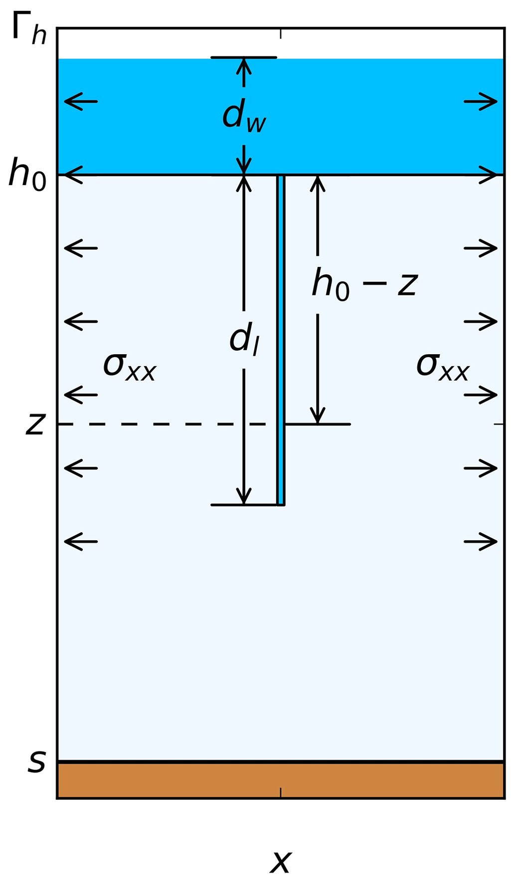
Figure 1 shows a schematic of the computational domain. We consider a segment of a marine ice sheet with length 2L and thickness H(x,t) in a Cartesian coordinate system, with position vector $\mathit{x}=\left(x,z\right)$, where z increases upward. The inflow and outflow boundaries are denoted Γ_in and Γ_out. The top surface is denoted Γ_h. The bottom surface is divided into two parts, according to whether the ice is in contact with the bedrock or the ocean. The ice–bedrock interface Γ_s is where the ice is in contact with the bedrock at a height b(x). As a simplification, we assume that the bedrock has a uniform slope θ. The ice–ocean interface Γ_w is where the ice is detached from the bedrock. The two boundaries, Γ_s and Γ_w, meet at the GL, whose horizontal position, denoted x_g(t), migrates with time t. The origin of the coordinate system is set at the middle of the domain on the ice–bedrock interface (at the position of the GL shown in Fig. 1).

Figure 1 Schematic showing the model domain of a marine ice-sheet system.

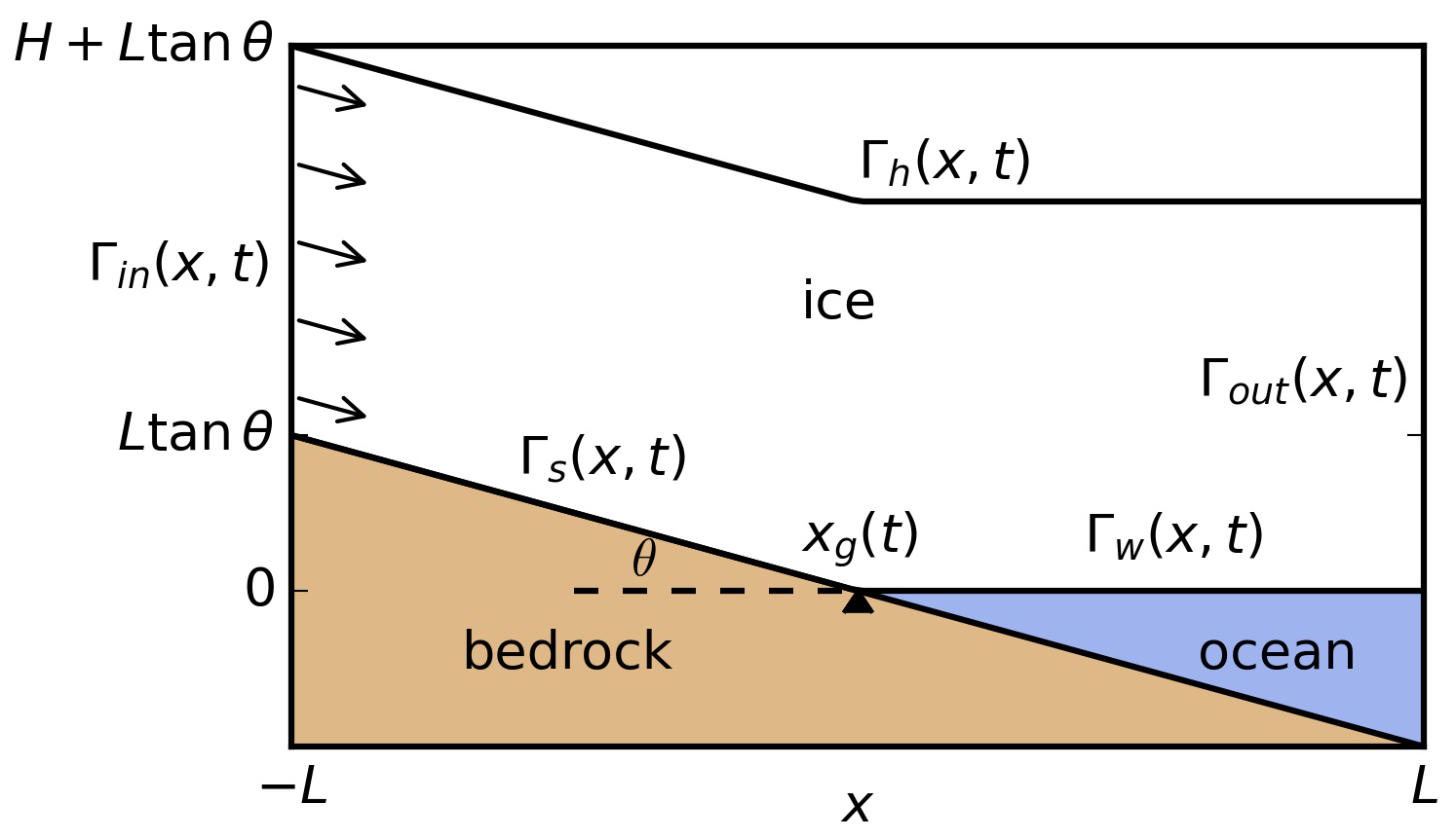
Following Stubblefield et al. (2021), we first construct the mesh with the piecewise linear bottom profile s(x) and surface profile h(x)

$$\begin{array}{ll}{\displaystyle }& {\displaystyle }s\left(x\right)=\text{max}\left(b\left(x\right),\mathrm{0}\right),\\ \text{(1)}& {\displaystyle }& {\displaystyle }h\left(x\right)=s\left(x\right)+H,\end{array}$$

which are shown in Fig. 1. We evolve this initial profile with no tides until the ice-flow geometry (i.e. s(x), h(x), and GL x_g) reaches a steady state. In practice, the ice flow reaches the steady state when the GL attains its steady position, defined as when its migration can not be resolved with the 25 m grid size. This provides a steady profile of the marine ice sheet for use as an initial condition for simulations with tides.

2.2 Governing equations

The governing equations for momentum and mass conservation are

$$\begin{array}{}\text{(2)}& {\displaystyle }& {\displaystyle }\mathbf{\nabla }\cdot \mathit{\sigma }+{\mathit{\rho }}_{\mathrm{i}}\mathit{g}=\mathbf{0},\text{(3)}& {\displaystyle }& {\displaystyle }\mathbf{\nabla }\cdot \mathit{u}=\mathrm{0},\end{array}$$

where σ is the total Cauchy stress tensor, ρ_i is ice density, g is gravity, and u is the ice velocity field. The stress σ can be decomposed as an isotropic part and a deviatoric part, $\mathit{\sigma }=-p\mathbf{I}+\mathit{\tau },$ where p and τ represent the pressure and deviatoric stress, respectively. Here, I is the unit tensor.

To model viscoelasticity, we adopt the upper-convected Maxwell formulation for the deviatoric stress τ. The constitutive relationship is

$$\begin{array}{}\text{(4)}& {\displaystyle }{\displaystyle }\mathit{\tau }+\mathit{\lambda }\stackrel{\nabla }{\mathit{\tau }}=\mathrm{2}\mathit{\eta }\dot{\mathit{\epsilon }},\end{array}$$

where the Maxwell time, $\mathit{\lambda }=\mathit{\eta }/\mathit{\mu }$, is the ratio of ice viscosity η to shear modulus μ. The strain rate is denoted $\dot{\mathit{\epsilon }}$. The upper-convected time derivative (Oldroyd rate) $\stackrel{\nabla }{\mathit{\tau }}$ measures the temporal variation of τ, including the effect of rigid body rotation,

$$\begin{array}{}\text{(5)}& {\displaystyle }{\displaystyle }\stackrel{\nabla }{\mathit{\tau }}={\partial }_t\mathit{\tau }+\mathit{u}\cdot \mathrm{\nabla }\mathit{\tau }-(\mathrm{\nabla }\mathit{u}{)}^{\mathrm{T}}\cdot \mathit{\tau }-\mathit{\tau }\cdot \mathrm{\nabla }\mathit{u},\end{array}$$

where (⋅)^T represents tensor transpose.

We assume a constant shear modulus μ and non-Newtonian viscosity η that is governed by Glen's flow law with regularisation

$$\begin{array}{}\text{(6)}& {\displaystyle }{\displaystyle }\mathit{\eta }={\displaystyle \frac{\mathrm{1}}{\mathrm{2}}}B\left(\right|\dot{\mathit{\epsilon }}{|}^{\mathrm{2}}+{\mathit{\delta }}_{\mathit{\nu }}{)}^{-(n-\mathrm{1})/\mathrm{2}n},\end{array}$$

where $B={\mathrm{2}}^{(n-\mathrm{1})/\mathrm{2}n}{A}_{\mathrm{0}}^{-\mathrm{1}/n}$ is determined by the two flow law parameters, A₀ and n, and $\left|\dot{\mathit{\epsilon }}\right|=\sqrt{\dot{\mathit{\epsilon }}:\dot{\mathit{\epsilon }}}$ is the Frobenius norm of the strain rate. Regularisation with the numerical parameter δ_ν is used to prevent infinite viscosity at a vanishing strain rate (Jouvet and Rappaz, 2011; Helanow and Ahlkrona, 2018; Stubblefield et al., 2021). The value of δ_ν sets an upper limit on the viscosity and, therefore, also on the Maxwell time. In our reference parameter set used below, $\mathit{\eta }\le \mathrm{1.3}\times {\mathrm{10}}^{\mathrm{14}}\mathrm{Pa}\mathrm{s}$ and λ≤120 h. For δ_ν=0, Eq. (6) reduces to the classical form of Glen's flow law.

2.3 Boundary conditions

Neglecting atmospheric pressure and other surface loading, the top boundary is assumed to be stress-free. Its elevation h is governed by the kinematic condition

$$\begin{array}{}\text{(7)}& {\displaystyle }{\displaystyle \frac{\partial h}{\partial t}}(x,t)={\left[{\left({\displaystyle \frac{\partial h}{\partial x}}\right)}^{\mathrm{2}}+\mathrm{1}\right]}^{\mathrm{1}/\mathrm{2}}\mathit{u}\cdot \mathit{n}\text{on }{\mathrm{\Gamma }}_h,\end{array}$$

where n is the outward-pointing unit normal vector, and Γ_h is the top boundary.

On the inflow boundary Γ_in, we impose a uniform horizontal inflow rate u₀ and zero shear stress

$$\begin{array}{}\text{(8)}& {\displaystyle }{\displaystyle }\left\{\begin{array}{l}\mathit{u}\cdot \mathit{n}=u_{\mathrm{0}},\\ \mathit{t}\cdot \mathit{\sigma }\cdot \mathit{n}=\mathrm{0},\end{array}\right.\text{on}{\mathrm{\Gamma }}_{\text{in}},\end{array}$$

where t is the tangential unit vector. The inflow velocity u₀ is set to be the satellite-derived surface velocity, 18 m yr⁻¹ (Rignot et al., 2016). On the outflow boundary, we impose the ice-overburden pressure

$$\begin{array}{}\text{(9)}& {\displaystyle }{\displaystyle }\mathit{\sigma }\cdot \mathit{n}=-{\mathit{\rho }}_{\mathrm{i}}g\left(h-z\right)\mathit{n},\text{on}{\mathrm{\Gamma }}_{\text{out}},\end{array}$$

which means that at the downstream boundary Γ_out, the ice shelf floats at hydrostatic equilibrium, without bending stress.

Similar to Eq. (7), the bottom profile s(x,t) is governed by the kinematic equation

$$\begin{array}{}\text{(10)}& {\displaystyle }{\displaystyle \frac{\partial s}{\partial t}}(x,t)=-{\left[{\left({\displaystyle \frac{\partial s}{\partial x}}\right)}^{\mathrm{2}}+\mathrm{1}\right]}^{\mathrm{1}/\mathrm{2}}\mathit{u}\cdot \mathit{n},\text{on }{\mathrm{\Gamma }}_{\mathrm{w}},\end{array}$$

where Γ_w is the ice–ocean interface. The stress on the bottom boundary depends on the local contact condition. To introduce the boundary conditions related to the contact problem, we consider the hydrostatic water pressure p_w on the ice–ocean interface, defined as

$$\begin{array}{}\text{(11)}& {\displaystyle }{\displaystyle }{p}_{\mathrm{w}}={\mathit{\rho }}_{\mathrm{w}}g\left[h_{\mathrm{w}}\left(t\right)-s^{*}\right],\text{on }{\mathrm{\Gamma }}_{\mathrm{w}},\end{array}$$

where ρ_w is water density, g is gravitational acceleration, h_w is the sea level, and s^* is the approximated bottom boundary that will be introduced in Sect. 2.4. Atmospheric pressure is neglected at the ice–ocean interface, as it is generally small compared to the hydrostatic pressure.

The sea level h_w is a superposition of a steady state h₀ and a sinusoidal function of time, representing ocean tides with amplitude A and frequency f,

$$\begin{array}{}\text{(12)}& {\displaystyle }{\displaystyle }{h}_{\mathrm{w}}\left(t\right)=h_{\mathrm{0}}+A\sin \left(\mathrm{2}\mathit{\pi }ft\right).\end{array}$$

On the ice–ocean interface, the hydrostatic pressure p_w is imposed as the traction

$$\begin{array}{}\text{(13)}& {\displaystyle }{\displaystyle }\mathit{\sigma }\cdot \mathit{n}=-p_{\mathrm{w}}\mathit{n},\text{on }{\mathrm{\Gamma }}_{\mathrm{w}}.\end{array}$$

On the ice–bedrock interface, ice can be either attached or detached from the bed. In the normal direction, the contact condition is established by the following boundary conditions

$$\begin{array}{}\text{(14)}& {\displaystyle }{\displaystyle }\left\{\begin{array}{l}{\mathit{\sigma }}_{\mathrm{n}}⩾p_{\mathrm{w}},\\ u_{\mathrm{n}}\le \mathrm{0},\\ \left({\mathit{\sigma }}_{\mathrm{n}}-p_{\mathrm{w}}\right)u_{\mathrm{n}}=\mathrm{0},\end{array}\right.\text{on }{\mathrm{\Gamma }}_{\mathrm{s}},\end{array}$$

where σ_n is the normal component of traction. Here, the water pressure p_w follows Eq. (11). When u_n=0, ice is attached to the bed, σ_n≥p_w. When u_n<0, ice is detached from the bed, thus σ_n=p_w. The impenetrability condition is implemented using the penalty term shown in Sect. 2.4, originally proposed by Stubblefield et al. (2021).

In the tangential direction, ice sliding is resisted by friction that is governed by a Weertman-type sliding law (Weertman, 1957)

$$\begin{array}{}\text{(15)}& {\displaystyle }{\displaystyle }\mathit{t}\cdot \mathit{\sigma }\cdot \mathit{n}=-C{\left[{\left(\mathit{u}\cdot \mathit{t}\right)}^{\mathrm{2}}+{\mathit{\delta }}_{\mathrm{s}}\right]}^{-\frac{n-\mathrm{1}}{\mathrm{2}n}}\mathit{u}\cdot \mathit{t}\text{on }{\mathrm{\Gamma }}_{\mathrm{s}},\end{array}$$

where C is the friction coefficient, δ_s is a numerical factor preventing singularity, and n is the exponent in Glen's flow law (Eq. 6). In the computation, we choose C such that the surface velocity at the GL matches the inflow speed u₀. This choice gives a relatively low surface velocity gradient, which aligns with satellite observations at the lake region (Rignot et al., 2016).

2.4 Numerical implementation

When implementing the hydrostatic water pressure on the ice–ocean interface, for numerical stability, rather than the bottom elevation from the previous time step, s^* is used as an approximation to the current step elevation (Durand et al., 2009; Stubblefield et al., 2021), defined as

$$\begin{array}{}\text{(16)}& {\displaystyle }{\displaystyle }{s}^{*}(x,t)=s(x,t-\mathrm{\Delta }t)-u_{\mathrm{n}}(x,s,t)\mathrm{\Delta }t,\end{array}$$

where Δt is the numerical time step, $s(x,t-\mathrm{\Delta }t)$ is the bottom profile at the previous time step, and u_n is the normal velocity at the bottom boundary (u_n>0 accounts for downward motion).

In the variational formulation, on the ice–bedrock interface, the contact condition (Eq. 14) is accounted for by imposing the hydrostatic pressure (Eq. 11) to basal ice, along with a line integral as a penalty term in the variational formulation

$$\begin{array}{}\text{(17)}& {\displaystyle }{\displaystyle \frac{\mathrm{1}}{\mathit{\epsilon }}}\underset{{\mathrm{\Gamma }}_{\mathrm{s}}}{\int }{\displaystyle \frac{\mathrm{1}}{\mathrm{2}}}\left(\mathit{u}\cdot \mathit{n}+\left|\mathit{u}\cdot \mathit{n}\right|\right)\mathit{v}\cdot \mathit{n}\mathrm{d}s,\end{array}$$

where ε is the penalty parameter, and v is the test function corresponding to the velocity field u. The penalty term (Eq. 17) becomes non-zero only when u_n>0, and, thus, it penalises penetration. For the viscous contact problem, when ε→0, the solution to the variational formulation weakly converges to the solution governed by the contact condition (Eq. 14) (Kikuchi and Oden, 1988). For the viscoelastic case, although the variational formulation cannot be directly cast as a minimisation problem for ε→0, this limit is still a good approximation to the solution governed by the contact condition.

The variational formulation is implemented using the finite-element library FEniCS (Logg and Wells, 2010; Logg et al., 2012; Langtangen and Logg, 2017). A mixed finite element is used to solve for a combined field $\left(\mathit{u},p,\mathit{\tau }\right)$. We use triangular elements in which the pressure varies linearly, and the velocity and deviatoric stress vary quadratically. We report convergence tests that show that the results are mesh-independent (Appendix A). Meanwhile, in the limit of no elastic deformation (μ→∞), the model results converge to the viscous solutions by Stubblefield et al. (2021) (Sect. 3). For further details about the variational formulation and its numerical implementation, the reader is referred to Stubblefield et al. (2021).

3 Results

We first present a reference case that illustrates the tidal response of an idealised marine ice sheet without lateral confinement. We consider a 20 km long section of a 500 m thick ice sheet, sliding on bedrock with constant bed slope angle θ=0.02 (Fig. 2). Initially, the grounded ice sheet and floating ice shelf each cover 10 km of the domain. In the model of elasticity, we use Young's modulus E=0.88 GPa and Poisson's ratio ν=0.41, as suggested by Vaughan (1995) for tidal flexure problems. A list of parameters and their reference values are provided in Table 1. The tidal amplitude A is chosen to be 1 m. Except for the lateral confinement, the idealised model is designed to mimic the real grounding zone reported in Trusel et al. (2022). Section 4 provides a detailed analysis of the remotely sensed ice velocity and stress within that specific grounding zone.

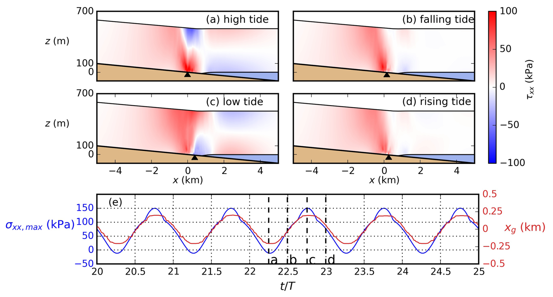
Figure 2 Tidal response of a marine ice sheet at different tidal phases. (a–d) Deviatoric tensile stress τ_xx in one tidal period, with red indicating tensile stress and blue indicating compressive stress. The black triangle marks the position of the GL. (e) The maximum tensile stress σ_xx,max (blue) on the top boundary within the lake region ($\overline{x_{\mathrm{g}}}-\mathrm{0.5}\mathrm{km}\le x\le \overline{x_{\mathrm{g}}}+\mathrm{0.5}\mathrm{km}$) and the GL position x_g (red) vs. time (scaled by the tidal period T) with positive values representing downstream migration. Vertical dashed lines show the time of panels (a–d).

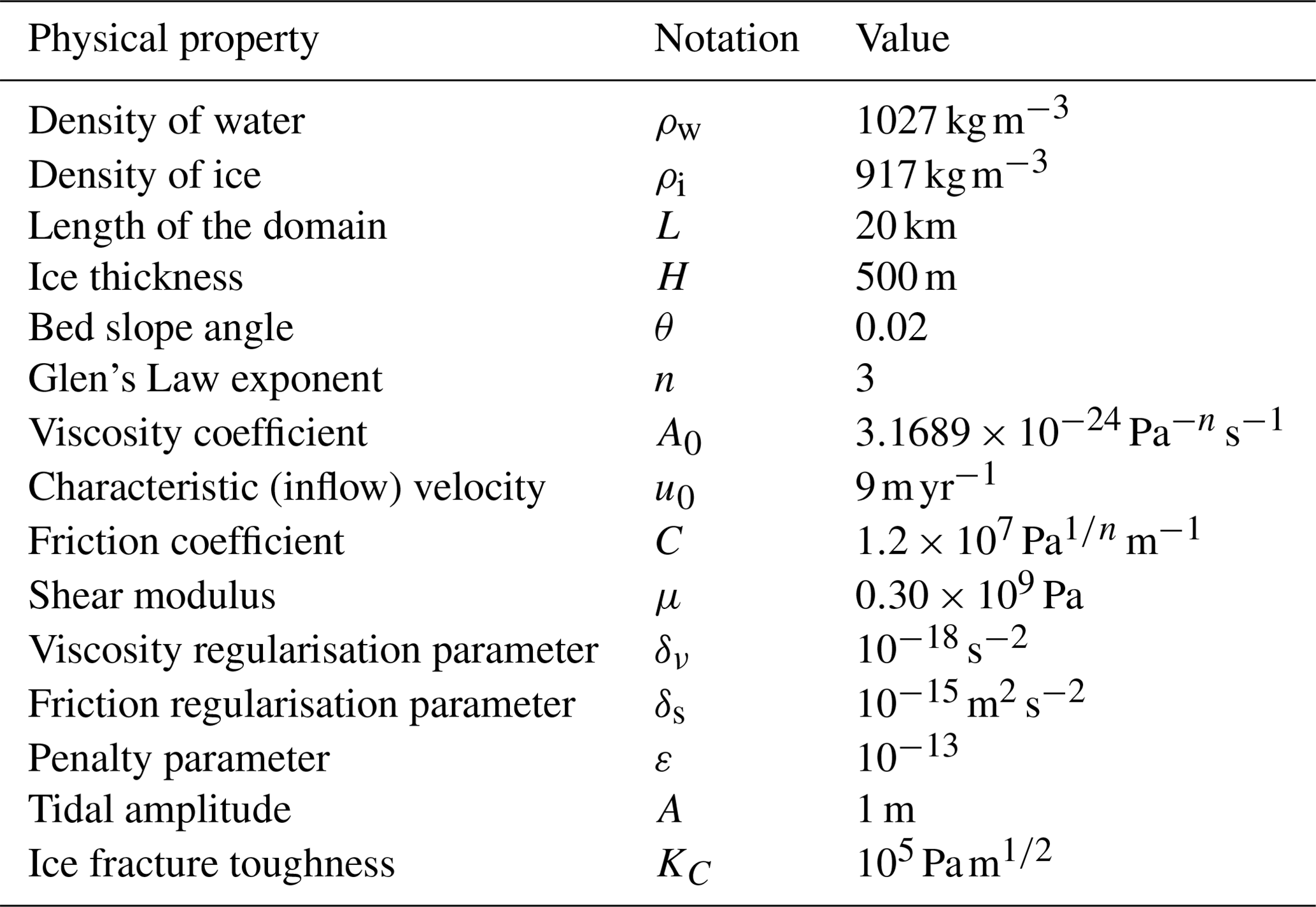
Table 1 Parameters used in the numerical model and their reference values.

3.1 Tidally induced grounding line migration and stress

As shown in Eq. (1), we first construct the mesh with a piecewise linear bottom profile and evolve this initial profile with no tides until the ice-flow geometry (i.e. s(x), h(x), and GL x_g) reaches a steady state. The steady profile is then used as an initial condition for simulations with tides.

We find tidally modulated GL migration and corresponding changes in stress. The GL position x_g is shown in Fig. 2e. While Stubblefield et al. (2021) find double GLs at low tides with a relatively small bed slope angle $\mathit{\theta }=\mathrm{2.5}\times {\mathrm{10}}^{-\mathrm{4}}$ (Stubblefield et al., 2021), in our model, we find only a single GL migrating in phase with the tides. This migration results in a 600 m wide grounding zone, which is larger than that estimated from hydrostatic equilibrium assuming a uniform ice thickness ($\mathrm{2}A/\mathit{\theta }=\mathrm{100}\mathrm{m}$).

To demonstrate tidal flexure, we plot the deviatoric stress component τ_xx at four tidal phases (Fig. 2a–d). The ice undergoes upward and downward flexure at high and low tides, respectively. At high tide (Fig. 2a), the stress is concentrated close to the GL, with compression near the top and tension near the bottom, immediately downstream of the GL. This resembles the stress pattern of a thin plate (Timoshenko, 1955), indicating a region where the ice vertical velocity transitions from the ice-sheet flow to the ice-shelf oscillation with tides. Further downstream, at the floating shelf, the stress is predominantly cryostatic without bending. At low tide (Fig. 2c), the tensile stress dominates the ice-sheet top surface near the GL. The region experiencing the tensile stress is more extensive and situated further upstream than during rising and falling tides. At rising tides (Fig. 2b) and falling tides (Fig. 2d), τ_xx is tensile at the GL, but the magnitude is smaller than τ_xx at low tide.

The full horizontal tensile stress σ_xx is considered for hydrofracturing at the lake. Assuming that the lake covers the ice-sheet surface within $|x-{\stackrel{\mathrm{‾}}{x}}_{\mathrm{g}}|\le \mathrm{0.5}\mathrm{km}$, where ${\stackrel{\mathrm{‾}}{x}}_{\mathrm{g}}$ is the time-averaged GL position in a tidal period, we calculate the maximum σ_xx on the ice-sheet surface within the lake region for any given time, which is denoted σ_xx,max. The temporal variation of σ_xx,max is shown in Fig. 2e. In each tidal period, σ_xx,max reaches its peak at low tide, corresponding to the downward flexural stress in Fig. 2c.

The reference case gives the tidal stress at tidal amplitude A=1 m. We further consider cases with a series of tidal amplitudes from 0 to 1 m, and thus obtain a stress–amplitude relationship for sinusoidal semi-diurnal tides, which we refer to as the “σ–A relationship” from this point forward. Specifically, this is the relationship between σ_xx,max at low tides and the tidal amplitude A, assuming that the sea-level variation due to tides follows a monochromatic sinusoid over time. However, with solar tides, tidal amplitude is modulated in a two-week cycle. Given that viscoelastic rheology has history dependence, such an amplitude modulation might complicate the σ–A relationship from monochromatic tides.

To explore the σ–A relationship with solar tides, we replace the sine function in Eq. (12) with a sine function whose amplitude is modulated over a 14 d period, with sea-level variation shown in Fig. 3. Applying this forcing to the reference case, the GL migrates in phase with tides (Fig. 3a). In each tidal period, the low-tide σ_xx,max tracks the σ–A relationship for sinusoidal tides, with slight discrepancies observed at small tidal amplitudes (Fig. 3b), indicating that solar tidal amplitude modulation does not change the σ–A relationship. Therefore, daily maximum tidal amplitude proves to be a good metric to estimate the daily maximum tidal stress that contributes to hydrofracturing.

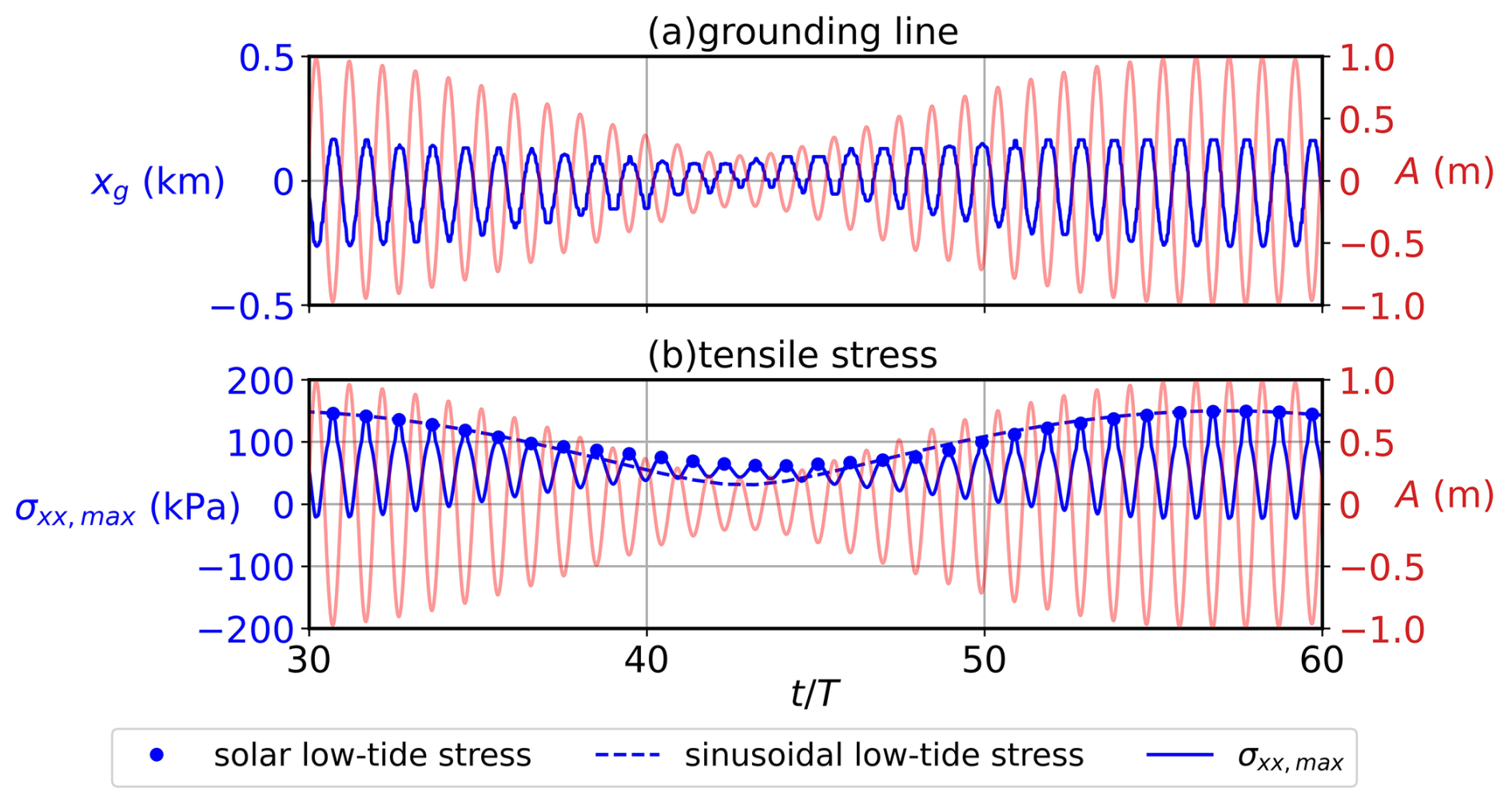
Figure 3 (a) Modulated tidal amplitude (red) and corresponding GL migration (blue). The horizontal axis is time scaled by the tidal period. (b) (blue) Maximum deviatoric tensile stress σ_xx,max on the ice-sheet surface within the lake region with modulated tidal amplitude. The dots denote the low-tide stress in one tidal period. The dashed blue line is the estimated low-tide stress calculated from the modulated tidal amplitude using the σ–A relationship from sinusoidal semi-diurnal tides in Sect. 3.1.

3.2 Sensitivity analysis

The viscoelastic model can be applied to other glaciers with different rheological properties and bed topography. Here, we analyse the model's sensitivity to ice viscoelasticity and bed topography. From this point forward, we use σ_xx,max to denote the low-tide maximum tensile stress within the lake region, which is assumed to directly contribute to hydrofracturing.

3.2.1 Sensitivity to the Deborah number

In a viscoelastic grounding zone, the tidal response is governed by the Deborah number (De), a dimensionless parameter defined as De = λf, where λ is the Maxwell time of ice and f is the tidal frequency. Depending on De, the tidal response is primarily elastic (De ≫1) or viscous (De ≪1). Here, we explore the tidal response across a range of De values, from 10⁻⁴ to 10², capturing the transition from viscous to elastic tidal response.

We vary De across two different parameterisation schemes, modifying the shear modulus μ or the prefactor A₀ in Glen's flow law. The variation in μ accounts for crevasses and damage that weaken the ice shelf, while changes in A₀ represents thermally controlled viscosity variations. All other parameters remain fixed at their reference values. We define a grounding-zone width, Δx_g, as the range of GL migration in a tidal period. In Fig. 4a, Δx_g is plotted against De. With the bed slope $\mathit{\theta }=\mathrm{2}\times {\mathrm{10}}^{-\mathrm{2}}$, a single GL is observed to migrate 0.5–1 km per tidal cycle. As μ→∞ (with $A_{\mathrm{0}}=\mathrm{1.2}\times {\mathrm{10}}^{-\mathrm{25}}{\mathrm{Pa}}^{-n}{\mathrm{s}}^{-\mathrm{1}}$), the tidal response becomes purely viscous, and the grounding-zone width converges to its viscous limit Δx_g,ν, exceeding the elastic regime. In contrast, increasing A₀ has a minimal effect on Δx_g. In Fig. 4b, as μ→∞, the low-tide maximum tensile stress within the lake region σ_xx,max increases and converges to the viscous stress calculated using the viscous model (Stubblefield et al., 2021). In contrast, as A₀ increases, the tidal stress slightly decreases due to the reduction in viscosity.

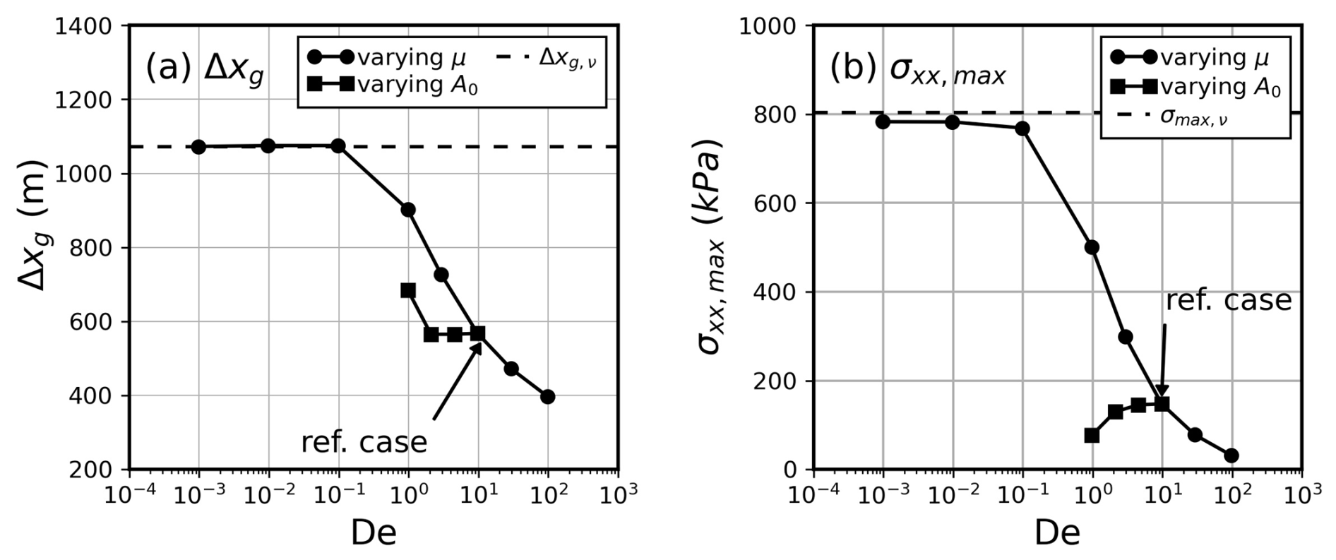
Figure 4 (a) The grounding-zone width Δx_g (solid lines), defined as $\mathrm{\Delta }{x}_{\mathrm{g}}=max\mathit{\left\{}{x}_{\mathrm{r}}\mathit{\right\}}-min\mathit{\left\{}{x}_{\mathrm{l}}\mathit{\right\}}$ as a function of De. We vary De by using two different schemes: (1) varying μ (round dots) from $\mathit{\mu }=\mathrm{3}\times {\mathrm{10}}^{\mathrm{7}}$ to 3×10¹² Pa; (2) varying A₀ (square dots) from $\mathrm{1.2}\times {\mathrm{10}}^{-\mathrm{25}}$ to $\mathrm{1.2}\times {\mathrm{10}}^{-\mathrm{22}}{\mathrm{Pa}}^{-\mathrm{3}}{\mathrm{s}}^{-\mathrm{1}}$. The dashed line is Δx_g,ν, the grounding-zone width in the viscous limit (μ→∞, $A_{\mathrm{0}}=\mathrm{1.2}\times {\mathrm{10}}^{-\mathrm{25}}{\mathrm{Pa}}^{-\mathrm{3}}{\mathrm{s}}^{-\mathrm{1}}$). (b) Maximum tensile stress σ_xx,max vs. De through a varying μ (round dots) or a varying A₀ (square dots). The dashed line is the tidal stress calculated by the viscous model (Stubblefield et al., 2021). The numerical reference case (Fig. 2) is labelled in both panels.

The Deborah number of ice is crucial in determining GL migration and tidal stress, because a dominantly viscous response tends to increase the width of the grounding zone and alter the magnitude of tidal stresses, compared with the elastic limit. Since the tidal period is well constrained, our model indicates the importance of using viscoelasticity with an appropriate Maxwell time to predict the magnitude of tidal stress. Given the dependence of Δx_g on De (Fig. 4a), it may be possible to infer ice mechanical properties from observations on the range of GL migration.

3.2.2 Sensitivity to bed slope angle

The above discussion shows how tidal response varies with shear modulus, given a characteristic bed slope $\mathit{\theta }=\mathrm{2}\times {\mathrm{10}}^{-\mathrm{2}}$ in the Amery Ice Shelf grounding zone. Here, we extend the results to different bed slopes and explore how the tidal response of a GL would change with local bathymetry. We consider three marine ice sheets with bed slope $\mathit{\theta }=\mathrm{2}\times {\mathrm{10}}^{-\mathrm{4}}$, $\mathrm{2}\times {\mathrm{10}}^{-\mathrm{3}}$, and $\mathrm{2}\times {\mathrm{10}}^{-\mathrm{2}}$, with all other parameters set to be the same as the reference case.

To simplify, we focus on the effect of θ while keeping the inflow velocity u₀ and the basal friction coefficient C in Eq. (15) fixed. Because of this, the ice adjusts to the changing bed slope through either thinning or thickening. The modelled surface velocity near the GL deviates from the observed value u₀, but it maintains the same order of magnitude. The GL migration is shown in Fig. 5a. Different from the single GL shown above, the low-bed-slope regime $\mathit{\theta }=\mathrm{2}\times {\mathrm{10}}^{-\mathrm{4}}$ is characterised by double GLs at low tides. Between the left GL at x_l and the right GL at x_r, the ice sheet is lifted due to a water layer trapped underneath, forming a “low-tide grounding zone” (Stubblefield et al., 2021). For the other two cases, only a single GL is found, with the range of the GL decreasing for increasing θ. Moreover, the maximum tidal stress monotonically increases with increasing θ (Fig. 5b). For a specific GL, the local basal topography and characteristic bed slope angle can be constrained through observations (Fretwell et al., 2013). Thus, the uncertainties of the modelled tidal GL migration and stress mainly come from the rheological model.

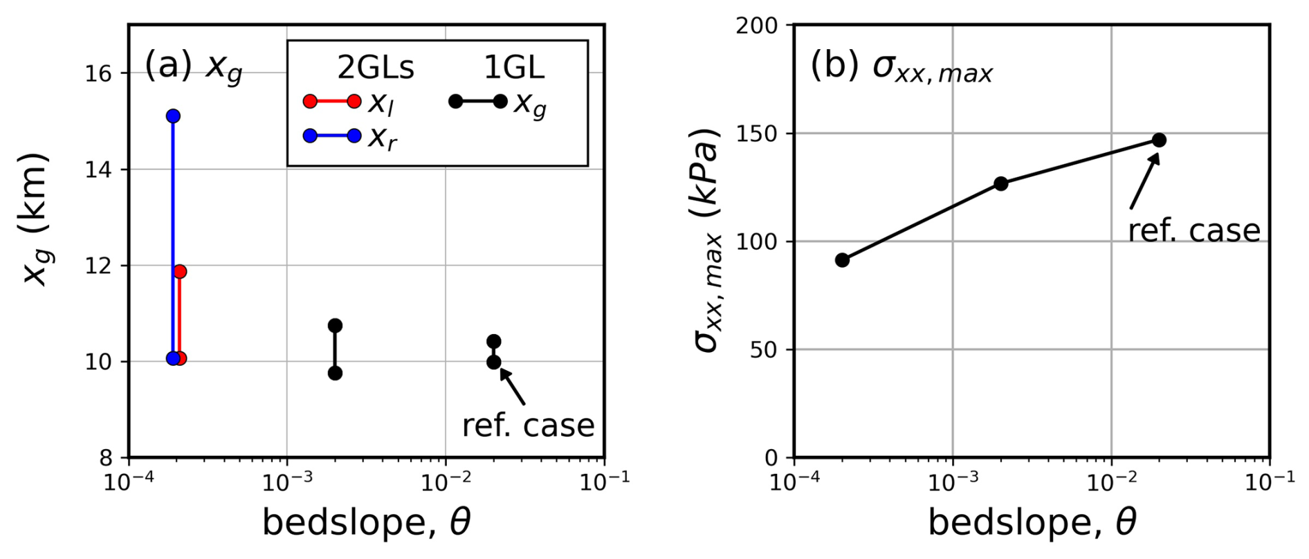
Figure 5 (a) The range of the GL position in one tidal period as a function of bed slope angle $\mathit{\theta }=\mathrm{2}\times {\mathrm{10}}^{-\mathrm{4}}$, $\mathrm{2}\times {\mathrm{10}}^{-\mathrm{3}}$, $\mathrm{2}\times {\mathrm{10}}^{-\mathrm{2}}$. When $\mathit{\theta }=\mathrm{2}\times {\mathrm{10}}^{-\mathrm{4}}$, there are two GLs. The left and right GLs are denoted x_l and x_r, respectively. The other two cases give single GL x_g shown by the black line. (b) Maximum tidal stress σ_xx,max vs. θ. The numerical reference case in Fig. 2 is labelled.

3.3 Linear elastic fracture mechanics model of the hydrofracture

The viscoelastic marine ice-sheet model enables the estimation of maximum tidal stress magnitudes within the grounding zone. In this section, through the application of a fracture mechanics framework, we demonstrate how this calculated tidal stress might drive surface hydrofracture propagation. Since hydrofracturing typically occurs on a timescale short enough that the surrounding ice behaves elastically, we consider fracture propagation in the LEFM framework. The hydrofracture is assumed to be a quasi-static elastic fracture occurring at the location with σ_xx,max at low tides. The stress that drives its propagation is the sum of the water pressure and tidal stress. The water pressure in the fracture p_w is assumed to be hydrostatic; the tidal stress σ_xx,max is calculated using the viscoelastic model mentioned above. We use the weight-function method to calculate the stress intensity factor K_I (Tada et al., 2000). Since at low tides the GL moves downstream and leaves the ice beneath the lake attached to the bedrock, we use a weight function that is designed for ice grounded on rigid bedrock, as suggested by Jimenez and Duddu (2018). Details about the calculation of K_I are provided in Appendix C.

Figure 6a shows a schematic of the fracture model. The lake basin has a depth d_b and is filled with water to a depth d_w. The horizontal stress σ_xx(z) represents the low-tide tidal stress and is obtained from the numerical results with a given tidal amplitude A. For a vertical fracture, we can calculate the stress intensity factor K_I as a function of its length d_l. If K_I exceeds the ice fracture toughness K_C, the fracture can propagate until K_I=K_C. We assume that lake drainage occurs when a vertical hydrofracture reaches the ice-sheet bottom.

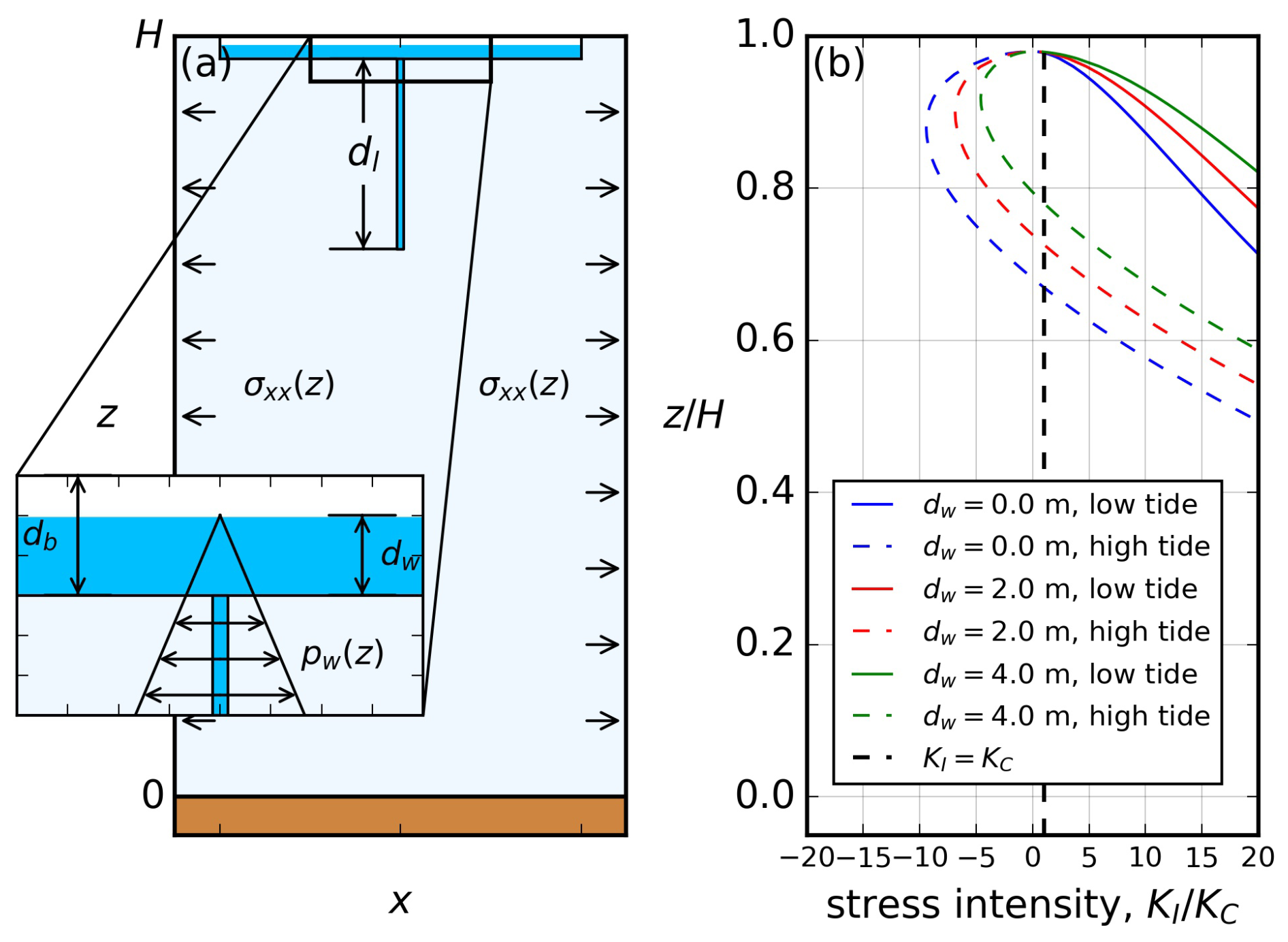
Figure 6 (a) The LEFM model of hydrofracture. The lake basin with depth d_b is filled with water to a depth d_w. Here, d_w serves as a measure of the water pressure p_w, as shown in the zoom-in window. Promoted by the tidal stress σ_xx(z) and lake-water pressure p_w, a vertical fracture with length d_l is initiated from the lake bottom. (b) A reference case showing $K_I/K_C$ varying with depth (scaled by the ice thickness) and tidal phases, with A=1.0 m, d_b=10 m, and $d_{\mathrm{l},\text{init}}=\mathrm{0.1}$ m. The solid lines represent $K_I/K_C$ at low tides. The dashed lines represent $K_I/K_C$ at high tides, when upward flexure causes compression and results in a negative tidal contribution to hydrofracture.

Note, for the initial fracture, K_I is sensitive to its length d_l,init. However, there is limited observational constraint on the lengths of pre-existing fractures in lake basins. While the choice of d_l,init requires further study, the relative importance of the lake pressure vs. the tidal amplitude is independent of d_l,init, which is shown in the model-based criterion below. Here, we will choose d_l,init such that the model criterion best fits the drainage data from Trusel et al. (2022). For an initial fracture with $d_{\mathrm{l},\text{init}}=\mathrm{0.1}$ m to propagate, the critical tensile stress is approximately σ_xx=150 kPa. For $d_{\mathrm{l},\text{init}}=\mathrm{0.2}$ m, the critical stress is about 100 kPa, which cannot be achieved by background extension alone in the reference case shown in Fig. 2.

Figure 6b shows a reference case with $K_I/K_C$ vs. the fracture length d_l, utilising the vertical stress distribution (σ_xx) derived from the numerical simulations in Sect. 3.1. We evaluate different combinations of lake depth d_w (d_w=0, 2, 4 m) and tidal phases (low tide and high tide). The vertical dashed line represents the ice fracture toughness K_C. During low tide, downward flexure generates positive K_I near the ice surface, whereas high-tide compressive stresses produce negative K_I at the same location. Figure 6b can be used to predict lake drainage: at low tides, for a pre-existing fracture with length d_l,init, if K_I>K_C holds for any depth that the fracture can reach, then A and d_w are predicted to induce lake drainage. By iteratively applying this criterion across combinations of A and d_w, we assess hydrofracture propagation likelihood for ranges of A and d_w values. This establishes a model-based drainage criterion within a two-dimensional parameter space defined by tidal amplitude (A) and lake depth (d_w). We discuss this model-based drainage criterion and its application to lake drainage in the Amery grounding zone in Sect. 4.2.

4 Discussion

In Sect. 3, we used a viscoelastic model to predict GL migration and tidal stress for a marine ice sheet, which was then integrated into a LEFM framework to assess tidally induced hydrofracturing. In the grounding zone analysed in Trusel et al. (2022), tidal responses could be more complex than predicted by the idealised flow-line model due to lateral stresses. Nevertheless, to our knowledge, the Trusel et al. (2022) dataset is the only observational record of tidally induced lake drainage that supports a quantitative analysis. In the following section, we first derive the strain-rate field near the lake studied by Trusel et al. (2022) using remotely sensed ice-surface velocity data. Then, we construct a model-based drainage criterion for laterally unconfined grounding zones, explicitly neglecting contributions from lateral stresses. We then test its predictions against the observations of Trusel et al. (2022). While the model-based criterion yields a prediction closely aligned with the data, deviations are observed. Finally, we discuss model limitations that could cause the deviations and propose potential refinements to extend the model's capability to laterally confined glaciers, which are important in governing the upstream ice-sheet mass balance.

4.1 Application to the Amery grounding zone: ice-flow field and lake-basin bathymetry

Trusel et al. (2022) report drainage characteristics for a supraglacial lake located at 70.59° S, 72.53° E. Figure 7a shows the ice-surface velocity field v from the MEaSUREs InSAR-Based Antarctica Ice Velocity Map (Rignot et al., 2011b, 2017; Mouginot et al., 2012, 2017), from which we calculate strain rates $\dot{\mathit{\epsilon }}$ and the ice-flow line that bisects the lake location. The lake is located on the GL position given by the MEaSUREs Antarctic Grounding Line from Differential Satellite Radar Interferometry, Version 2 (Rignot et al., 2016, 2011a, 2014; Li et al., 2015). We use BedMachine Antarctica v2 to obtain the basal topography and ice geometry along the flow line (Fig. 7b) (Morlighem et al., 2017, 2020). The subglacial cavity downstream of the grounding zone is more than 20 m in height, which is large enough to allow free tidal oscillation without the formation of pinning points. Thus, we assume that the ice shelf downstream of the GL does not contact the bedrock, and that the water pressure on the ice–ocean interface is hydrostatic. In the computation, we use a linear bedrock topography (Fig. 7b) with a slope angle chosen to approximately match observations. In Appendix B, we present model results with real bed topography for comparison.

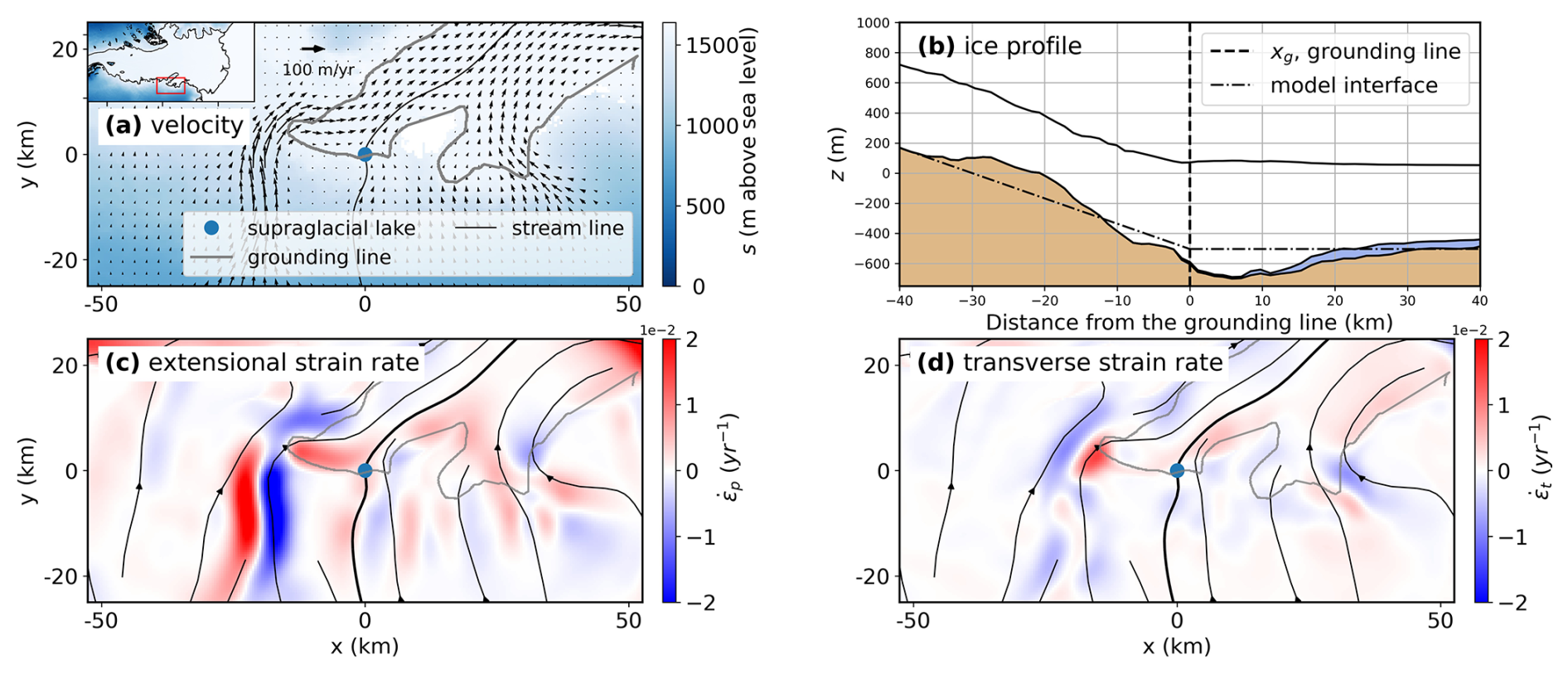
Figure 7 Ice surface velocity and strain rate in the region of the supraglacial lake. (a) Velocity field near the grounding line (grey), where the supraglacial lake is denoted with the blue dot. The solid black line is the streamline flowing through the lake location. The colour represents the ice-sheet surface elevation above sea level. The map inset at the top left corner shows ice-surface elevation for the full Amery Ice Shelf, with the plotted region outlined with a red box; (b) ice-sheet geometry and bed topography along the streamline in panel (a). Note that $x=x_{\mathrm{g}}=\mathrm{0}$ is the position of the supraglacial lake as well as the grounding line. The dash-dotted line is the idealised ice-bottom profile used in the model; (c) along-flow strain rate with positive values representing extension; (d) transverse strain rate.

Following Wearing (2017), we decompose the ice strain rate into an along-flow component and a transverse component. For each grid point, we compute the ice velocity orientation, defining the along-flow and transverse directions using unit vectors $\widehat{\mathit{v}}$ and $\widehat{\mathit{t}}$, respectively, within a local right-handed coordinate system. The along-flow strain rate is then derived pointwise as

$$\begin{array}{}\text{(18)}& {\displaystyle }{\displaystyle }{\dot{\mathit{\epsilon }}}_{\mathrm{p}}=\widehat{\mathit{v}}\cdot \dot{\mathit{\epsilon }}\cdot \widehat{\mathit{v}},\end{array}$$

and the transverse strain rate is

$$\begin{array}{}\text{(19)}& {\displaystyle }{\displaystyle }{\dot{\mathit{\epsilon }}}_{\mathrm{t}}=\widehat{\mathit{v}}\cdot \dot{\mathit{\epsilon }}\cdot \widehat{\mathit{t}}.\end{array}$$

Figure 7c and d shows ${\dot{\mathit{\epsilon }}}_{\mathrm{p}}$ and ${\dot{\mathit{\epsilon }}}_{\mathrm{t}}$ near the lake. The background stress is dominantly extensional away from the GL. However, near the Amery Ice Shelf shear margin, the ice flow deflects rightward, inducing a transverse strain-rate component. Meanwhile, upstream of the GL, the outlet glacier undergoes lateral shear that could modulate the along-flow momentum balance and the GL position. In our model, we focus on the extensional stress along the flow line and neglect factors related to lateral stresses.

To estimate the contribution from lake-water supply to hydrofracturing, we need to estimate the hydrostatic pressure at the bottom of the lake basin. To do so, we obtain the elevation of the basin from a 2 m resolution WorldView-1 DEM captured when the lake was dry. The elevation of the flat basin, excluding any craters or hydrofractures, is considered the lowest point of the lake. The basin is approximately 10 m deeper than the surrounding terrain and spans about 1 km in the direction perpendicular to the GL. The lake-water depth prior to each drainage event is calculated by subtracting the lake-basin elevation from the median shoreline elevation, which we obtain using the shoreline extraction technique outlined in Moussavi et al. (2016) and Trusel et al. (2022).

4.2 Application to the Amery grounding zone: drainage criteria from tidal amplitude and lake depth

In Sect. 3.3, we introduced how we construct the model-based criterion in the two-dimensional parameter space defined by tidal amplitude (A) and lake depth (d_w). The criterion corresponds to the marginal threshold at which an initial fracture propagates to the ice–bedrock interface. In Fig. 8a, we show two such criteria (denoted by square markers) for initial crack lengths of $d_{\mathrm{l},\text{init}}=\mathrm{0.1}$ and 0.2 m. When the parameter pair (A,d_w) of a lake crosses the criterion from bottom-left to top-right, the total tensile stress becomes large enough to enable hydrofracture penetration to the ice-sheet base. An increasing A reduces d_w along the criteria. This inverse relationship quantifies the relative importance of tidal flexure to water pressure in driving lake drainages through hydrofracturing. It suggests that, in the grounding zones of laterally unconfined ice shelves, ocean tides cause tidal flexure, which reduces the lake depth required for drainage through hydrofracturing.

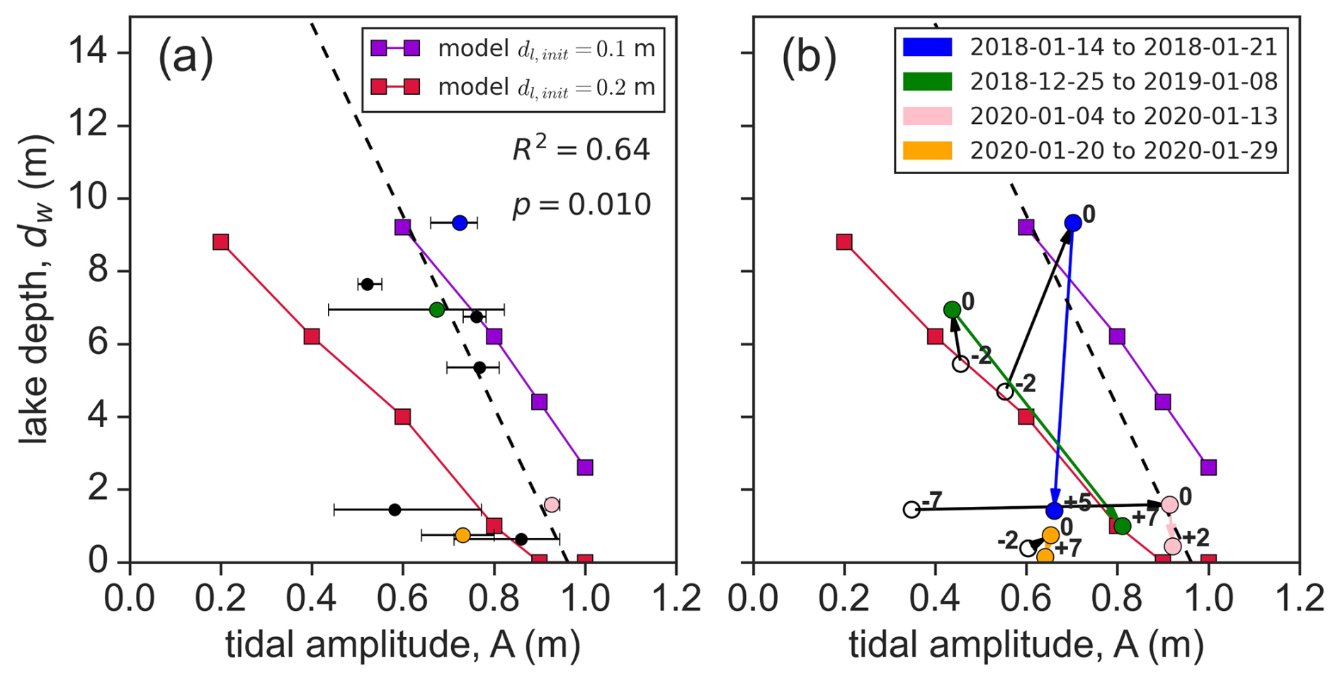
Figure 8 (a) A comparison between the model criterion and the drainage data. Each circle represents one drainage event from Trusel et al. (2022). The horizontal coordinate is the time-averaged daily maximum tidal amplitude during the drainage, with an error bar representing the range of the daily maximum tidal amplitude. The vertical coordinate is the pre-drainage lake depth. The dashed black line is a weighted linear regression of the observations. The red and violet lines are model-based criteria with different initial crack lengths, with squares representing the numerical experiments. The four coloured circles represent drainage events with best-constrained temporal evolution of lake depth and tidal amplitude. (b) Temporal evolution of coloured events in panel (a). The points labelled “0” represent the day of the drainage. The negative and positive values represent the days before and after the drainage, respectively.

Furthermore, the criterion identifies a critical A beyond which fracture propagation can occur solely due to tidal flexure and, hence, independently of water supply. When A is beyond this threshold, supraglacial lakes are unlikely to form because tidally driven flexure would open fractures in the grounding zone. Such fractures may act as vertical conduits, transporting surface water to the bed and preventing the meltwater accumulation that forms supraglacial lakes. These hypotheses can be tested by studying more supraglacial lake drainage events with tidal amplitude measured locally.

In Fig. 8a, we compare the model-based criterion with data from Trusel et al. (2022). The data cluster close to the model-based criterion for $d_{\mathrm{l},\text{init}}=\mathrm{0.1}$, 0.2 m. A weighted linear regression of the observations suggests that a higher tidal amplitude reduces the lake depth required for drainage, indicating the importance of tidal flexure in driving hydrofracturing, as shown in our model. However, the steeper slope of the regression line suggests that the dependence of lake drainage on tidal amplitude is stronger than predicted by our model.

To better demonstrate the drainage process, Fig. 8b shows four events that have the best observational constraint on the temporal evolution of lake depth and tidal amplitude. We show measurements from before, during, and after the drainage. Note that we simply assume that the drainage occurs at the highest water level observed, which is the minimum pre-drainage water level due to the time interval between satellite images. The two events, dated 25 December 2018 and 4 January 2020, cross the criterion with $d_{\mathrm{l},\text{init}}=\mathrm{0.2}$ m during the observational interval of several days. The event dated 4 January 2018 crosses both criteria. The post-drainage states are below the criterion with $d_{\mathrm{l},\text{init}}=\mathrm{0.1}$ m, representing the end of drainage due to insufficient water supply.

4.3 Limitations

Deviations between the model-based criterion and the data regression indicate that we may be underestimating the tidal contribution to hydrofracturing (Fig. 8). As indicated at the beginning of Sect. 4, this could be due to the model not including the effects of lateral stresses in the grounding zone, which could alter the tidal response. To address this in future work, the lateral shear stress can be parameterised by an additional term in the along-flow momentum equilibrium equation (Eq. 2),

$$\begin{array}{}\text{(20)}& {\displaystyle }{\displaystyle }{\mathit{\tau }}_{\mathrm{w}}\sim {\displaystyle \frac{|u{|}^{\mathrm{1}/n-\mathrm{1}}}{W^{\mathrm{1}/n+\mathrm{1}}}},\end{array}$$

where u is the along-flow ice velocity, and W is the half-width of the glacier (e.g. Schoof, 2007a).

In addition, we assume a stress-free top surface in the viscoelastic flow model. However, the supraglacial lake can induce additional stress in the surrounding ice, particularly on floating portions of the grounding zone that allow downward flexure (MacAyeal and Sergienko, 2013). Meanwhile, fatigue due to stress oscillations can weaken ice strength and promote hydrofracturing (Borstad et al., 2012; Lhermitte et al., 2020). A better approach may be to consider the supraglacial lake and the ice damage directly within a 2-D viscoelastic model.

Another limitation arises from our assumption of hydrostatic water pressure on the ice–ocean interface. The pressure gradient induced by tidally modulated subglacial water flow can cause elastic flexure in ice sheets close to the grounding line (Warburton et al., 2020). Furthermore, ocean tides can change the effective pressure at the bed and lubricate the ice–bedrock interface, leading to a variation in basal friction that is not accounted for by the sliding law in our model (Gudmundsson, 2011). Thus, it is important to incorporate subglacial hydrology in simulating the tidal response of a marine ice sheet.

Limitations also arise from the lack of data availability. Relative to the tidal period and lake-drainage period, the lower temporal resolution of the remotely sensed observations might obscure the true lake depth and tidal amplitude at the time of drainage. Field measurements and satellite images of supraglacial lake drainage with a higher observational frequency could improve our understanding of tidally induced drainage.

5 Conclusions

Our study of tidally induced stress and hydrofracture propagation in a laterally unconfined, viscoelastic, marine ice-sheet grounding zone suggests that ocean tides can generate significant stress near the grounding line. These stresses can increase the vulnerability of ice sheets to hydrofracturing in grounding zones where lakes form. We further establish a model-based criterion for lake drainage that links ocean tides and lake depth to supraglacial lake drainage via hydrofracture. Importantly, the criterion indicates that tidal flexure reduces the critical lake depth required for drainage through hydrofracturing. While our model formulation simplifies the ice momentum balance by neglecting lateral shear stress, this study provides the first integrated assessment of tidally induced viscoelastic grounding line dynamics and fracture propagation, which helps to explain the role of ocean tides in driving grounding line migration and supraglacial lake drainage in marine ice sheets.

Appendix A: Convergence test

The convergence test shows that the results are mesh-independent. Here, we apply the same flow law parameter values, with $A_{\mathrm{0}}=\mathrm{3.2}\times {\mathrm{10}}^{-\mathrm{24}}{\mathrm{Pa}}^{-\mathrm{3}}{\mathrm{s}}^{-\mathrm{1}}$ and n=3 as (Stubblefield et al., 2021). Considering a marine ice sheet with bed slope $\mathit{\theta }={\mathrm{10}}^{-\mathrm{3}}$ and friction coefficient $C=\mathrm{7}\times {\mathrm{10}}^{\mathrm{5}}$, we use the fine-grid solution x_g, e, σ_e (Δx=6.25 m) as the exact solution. All other parameters are kept same as the reference case. Here, x_g, e denotes the time series of the exact GL position, and σ_e denotes the time series of the exact maximum tensile stress on the ice-sheet surface within the lake region $|x-{\overline{x}}_{\mathrm{g}}|\le \mathrm{0.5}\mathrm{km}$. As Δx decreases, the GL position x_g and maximum tensile stress σ_xx,max linearly converge to the fine-grid solution (Fig. A1).

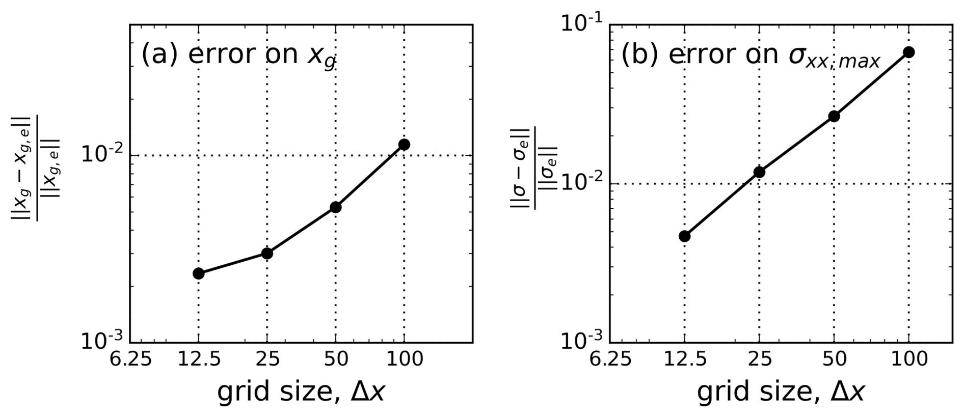
Figure A1 Convergence of (a) GL position and (b) maximum tensile stress σ_xx,max with decreasing element size Δx (12.5, 25, 50, 100 m). For simplicity, we denote σ_xx,max by σ. Here, x_g, e and σ_e denote the exact solution to the GL position and maximum tensile stress σ_xx,max, respectively. $\left|\right|\cdot \left|\right|$ is the L² norm.

Appendix B: Simulation with real bed topography

In Fig. B1, we present model results using the real bed topography shown in Fig. 7b (Morlighem et al., 2017, 2020). For comparison, the physical properties of ice and basal slipperiness C are kept the same as in idealised models with a linear bed. The jagged variation of x_g(t) is a consequence of the use of coarse grids near the grounding line for convergence. While the tidal stress and grounding-zone width are modified by bed undulation, the results have an equivalent order of magnitude to the case with linear bed topography, indicating the importance of tidal stress regardless of bed roughness. Therefore, we use the linear bed topography in the model.

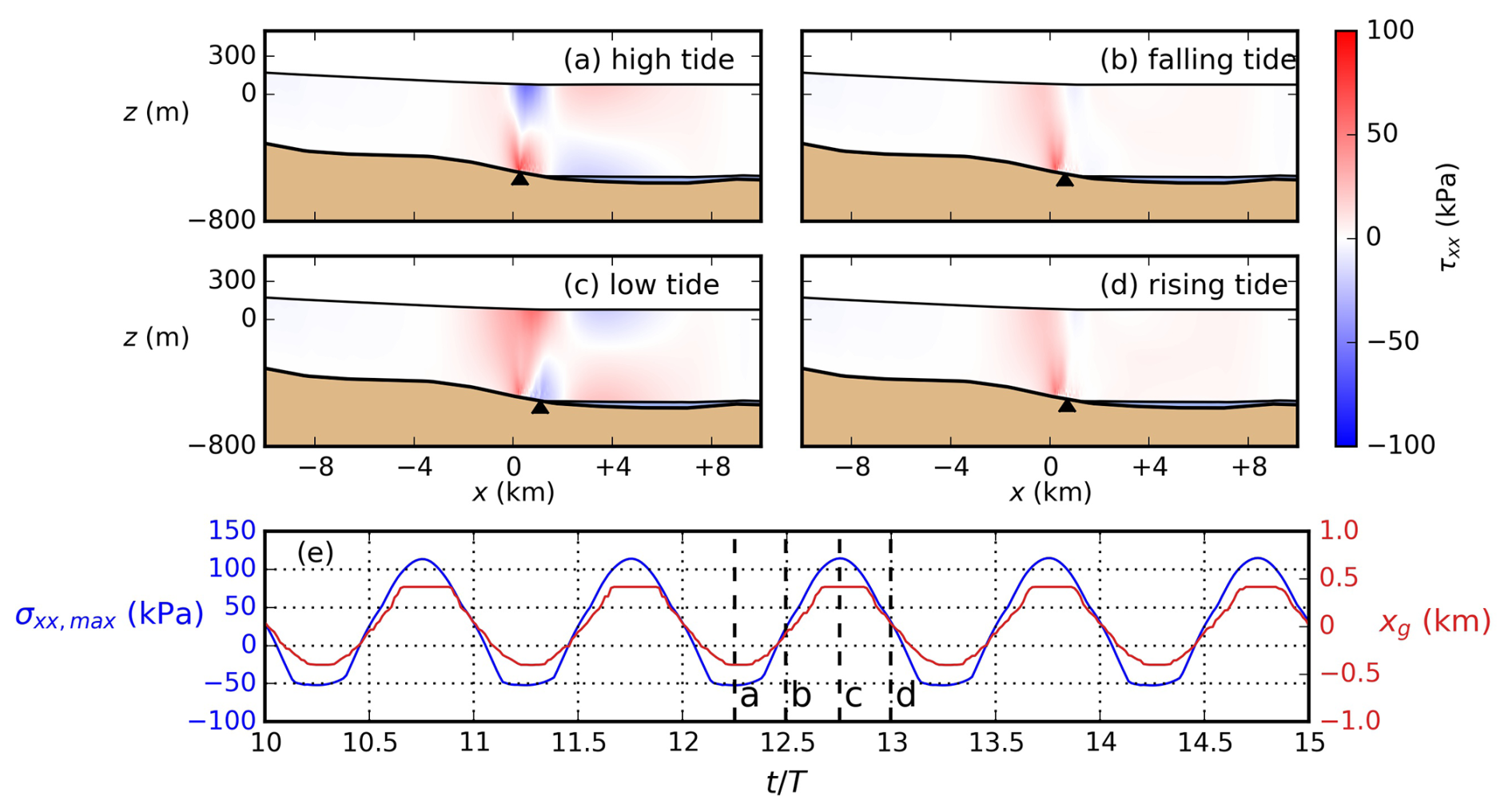
Figure B1 Tidal response of the ice shelf with real bed topography around the lake reported in Trusel et al. (2022). (a–d) Deviatoric tensile stress τ_xx in one tidal period. (e) The maximum tensile stress σ_xx,max (blue) on the top boundary within the lake region ($\overline{x_{\mathrm{g}}}-\mathrm{0.5}\mathrm{km}\le x\le \overline{x_{\mathrm{g}}}+\mathrm{0.5}\mathrm{km}$) and the GL position x_g (red) vs. time (scaled by the tidal period T) with positive values representing downstream migration. Vertical dashed lines show the time of panels (a–d).

Appendix C: Weight function method

In this Appendix, we introduce the weight function method to calculate the stress intensity factor K_I of a vertical surface hydrofracture of length d_l. Figure C1 shows the schematic of the fracture and weight function method. The stress contributing to hydrofracturing is denoted ${\mathit{\sigma }}_f={\mathit{\sigma }}_{xx}+p_{\mathrm{w}}$, which combines the net stress σ_xx from the model with the internal water pressure p_w(z) within the fracture. Assuming hydrostatic conditions, the water pressure p_w(z) is given by $p_{\mathrm{w}}\left(z\right)={\mathit{\rho }}_{\mathrm{w}}g\left(d_{\mathrm{l}}+d_{\mathrm{w}}\right)$, where d_w is the water depth of the lake. Here, the ice stress σ_xx(z) represents the vertical stress distribution at the location where the maximum surface horizontal tensile stress σ_xx,max is observed.

The factor K_I(d_l) is then computed by integrating σ_f along the fracture using a weight function G₁ (Tada et al., 2000),

$$\begin{array}{}\text{(C1)}& {\displaystyle }{\displaystyle }{K}_I\left(d_{\mathrm{l}}\right)=\underset{h_{\mathrm{0}}-d_{\mathrm{l}}}{\overset{h_{\mathrm{0}}}{\int }}{\mathit{\sigma }}_f\left(z\right)G_{\mathrm{1}}\left({\displaystyle \frac{d_{\mathrm{l}}}{H}},{\displaystyle \frac{h_{\mathrm{0}}-z}{d_{\mathrm{l}}}}\right)\mathrm{d}z,\end{array}$$

where $h_{\mathrm{0}}={\mathrm{\Gamma }}_h-d_{\mathrm{b}}$ is the lake basin elevation, $d_{\mathrm{l}}/H$ is the fracture length scaled by local ice thickness H, and $(h_{\mathrm{0}}-z)/d_{\mathrm{l}}$ denotes the depth below the lake basin, scaled by d_l. The weight function G₁ accounts for the surface hydrofracturing within an ice sheet located on a rigid bedrock (Jimenez and Duddu, 2018),

$$\begin{array}{ll}{\displaystyle }& {\displaystyle }{G}_{\mathrm{1}}\left(\mathit{\lambda },\mathit{\gamma }\right)={\displaystyle \frac{\mathrm{2}}{\sqrt{\mathrm{2}H}}}\\ {\displaystyle }& {\displaystyle }\times \sqrt{{\displaystyle \frac{\tan \left(\frac{\mathit{\pi }\mathit{\lambda }}{\mathrm{2}}\right)}{\mathrm{1}-{\left(\cos \frac{\mathit{\pi }\mathit{\lambda }}{\mathrm{2}}/\cos \frac{\mathit{\pi }\mathit{\lambda }\mathit{\gamma }}{\mathrm{2}}\right)}^{\mathrm{2}}}}}\mathit{\{}\mathrm{1}+\mathrm{0.3}\sqrt{\mathrm{1}-{\mathit{\gamma }}^{\mathrm{5}/\mathrm{4}}}\\ \text{(C2)}& {\displaystyle }& {\displaystyle }\times \left[\mathrm{0.5}\left(\mathrm{1}-\sin {\displaystyle \frac{\mathit{\pi }\mathit{\lambda }}{\mathrm{2}}}\right)\left(\mathrm{2}+\sin {\displaystyle \frac{\mathit{\pi }\mathit{\lambda }}{\mathrm{2}}}\right)\right]\mathit{\}}.\end{array}$$

Figure C1 Schematic of the fracture geometry used in the weight function method.