Evaluation of the Snow Climate Change Initiative (Snow CCI) snow-covered area product within a mountain snow water equivalent reanalysis

An accurate characterization of global snow water equivalent (SWE) is essential in the study of climate and water resources. The current global SWE dataset from the European Space Agency Snow Climate Change Initiative (Snow CCI) is derived from the assimilation of passive microwave satellite data and in situ snow depth measurements. However, gaps exist in the current Snow CCI SWE dataset in complex terrain due to difficulties in characterizing mountain SWE via the passive microwave sensing approach and limitations of the in situ snow depth measurements. This study applies a Bayesian snow reanalysis approach with the existing Snow CCI snow cover fraction (SCF) dataset (1 km resolution) to develop a SWE dataset over four mountainous domains in western North America for water years (WYs) 2001–2019. The reanalysis SWE estimates are evaluated through comparisons with independent SWE datasets and a parallel SWE reanalysis generated using snow extent retrieved from Landsat imagery (30 m resolution). Biases in Snow CCI reanalysis SWE were diagnosed by comparing Snow CCI snow cover with the Landsat reference. Both the number of SCF images and their characteristics (such as zenith angle) significantly affect the accuracy of SWE estimation. Overall, the Snow CCI SCF inputs produce reanalysis SWE of sufficient quality to fill the mountain SWE gap in the current Snow CCI SWE climate data record. A better characterization of the SCF uncertainty and a bias correction could further improve the accuracy of the reanalysis SWE estimates.

1 Introduction

Seasonal snowpack in mountainous regions plays a vital role in the global energy and water cycle. The unique properties of snow, such as its high albedo and low thermal conductivity, make it a significant factor in the energy budget of the lower atmosphere and Earth's surface. The seasonal snowpack conditions also influence the local weather and monsoon circulations (Rudisill et al., 2021). Furthermore, mountains act as natural water reservoirs, often referred to as “water towers”, by storing water in the form of snowpack and glaciers at high altitude (Immerzeel et al., 2020). It is estimated that between 50 % and 70 % of the annual precipitation in the mountainous regions of the western United States (WUS) falls as snow and is stored in the snowpack. During warmer seasons, this stored water is released as snowmelt, crucial for meeting downstream water demands and sustaining ecosystems. Many major rivers worldwide, such as the Colorado (spanning the United States and Mexico), Indus (flowing through the Himalaya), and Mackenzie (in Canada), heavily rely on mountain snowmelt. Such water towers are vulnerable to climatic and socio-economic changes, which can cause negative impacts on the ∼2 billion people (22 % of global populations) living downstream (Immerzeel et al., 2020; Mankin et al., 2015). Monitoring and managing the water resources from mountain snowpacks require accurate snow water equivalent (SWE) information. However, recent studies indicate that large discrepancies exist in the climatology of seasonal SWE magnitude and timing across different global datasets (Fang et al., 2023; Liu et al., 2022; Wrzesien et al., 2019; Mudryk et al., 2024; Kim et al., 2021) with uncertainty particularly high in mountain areas.

The European Space Agency (ESA) Snow Climate Change Initiative (Snow CCI) has developed homogenized, high-quality long-term snow cover fraction and SWE datasets to contribute to the understanding of snow in the climate system. In its initial phase, the Snow CCI project focused on generating consistent multi-sensor time series of daily fractional snow cover from optical satellite data (Nagler et al., 2022) and SWE derived from the assimilation of passive microwave (PM) satellite data and in situ snow depth. Snow CCI SWE data adopted the GlobSnow (v3) algorithm, which estimates SWE by combining PM brightness temperatures centered on 19 and 37 GHz from the Scanning Multichannel Microwave Radiometer (SMMR), Special Sensor Microwave/Imager (SSM/I), and Special Sensor Microwave Imager/Sounder (SSMIS) with in situ daily snow depth measurements via Bayesian non-linear iterative assimilation (Luojus et al., 2021).

The Snow CCI SWE product (and predecessor GlobSnow versions originally described in Takala et al., 2011) does not provide data over complex terrain because the coarse grid spacing (12.5 to 25 km) of the Snow CCI SWE product is incompatible with the scales of SWE variability in complex terrain. The Snow CCI SWE retrieval approach of combining satellite passive microwave measurements with surface snow depth measurements is not well suited to the complex terrain and deep snow typical of mountain regions because (1) the passive microwave sensitivity to SWE saturates when SWE exceeds 150 mm (Chang et al., 1982, 1987) and (2) the available snow depth observations are too sparse to meaningfully capture elevation and topographic variability in snow depth distribution (Pulliainen, 2006).

This study is motivated by the need to fill the mountain SWE gap in the Snow CCI SWE product. Specifically, we explore the use of a Bayesian snow reanalysis framework (BSRF) previously implemented in various mountain regions across the globe including the Sierra Nevada, the Andes, and High Mountain Asia (Margulis et al., 2016; Cortés et al., 2016; Liu et al., 2021; Fang et al., 2022). The framework combines prior snow estimates from an ensemble of land surface model simulations with satellite-derived fractional snow-covered area (fSCA) to generate retrospective time series of snow extent and SWE (Margulis et al., 2019). The previous implementations have used the Landsat-based fSCA product (Painter et al., 2003; Cortés et al., 2014) and the MODIS-based MODSCAG fSCA product (Painter et al., 2009; Margulis et al., 2019). Because a snow cover fraction product (MODIS-based) also exists within the Snow CCI program, it is a natural choice to use it to develop a mountain SWE product within the same program. There exist numerous snow cover datasets at various resolutions developed using different input data and retrieval approaches that provide differing fSCA values and error characteristics, such as the MODIS-based MOD10 snow cover fraction (SCF) product (Hall and Riggs, 2016). This study focuses on evaluating one such product – Snow CCI SCF, hereafter referred to as Snow CCI fSCA – within the BSRF framework to maintain consistency with the overall Snow CCI development framework and objectives. The primary objective of this study is to evaluate whether using the Snow CCI fSCA product within the BSRF can provide meaningful SWE estimates in mountain terrain. The Snow CCI fSCA products are global in coverage, so this approach can potentially be extended to all mountain regions in the future. We evaluate this objective by implementing the product across four test watersheds. Two watersheds are in the WUS where the BSRF was already previously implemented using Landsat (Fang et al., 2022). For these regions we can compare the established performance of the Landsat implementation to performance when using the Snow CCI fSCA in order to characterize how differences in the fSCA products result in different SWE estimates. We also implement the BSRF with Snow CCI fSCA data in two new watersheds in Canada. By extending the BSRF to a new region of the globe we have an opportunity to assess challenges that would arise in a global implementation of the BSRF. The remainder of this paper is organized as follows. Section 2 describes the methods, data, and application domain; Sect. 3 provides results and discussion; and Sect. 4 provides the key conclusions of the study.

2 Data, application domains, and methods

2.1 Description of the Snow CCI fSCA product

The Snow CCI fSCA dataset is globally available at a spatial resolution of 0.01° (∼1 km). The 1 km resolution of the Snow CCI fSCA product is relatively coarse compared to the resolution of available optical imagery but is well suited to the potential application across all Northern Hemisphere mountain areas for gap filling the existing Snow CCI SWE product. This study uses the MODIS-based Snow CCI Daily fSCA product (version 2), available over the period 2000–2020 (http://cci.esa.int/data, last access: 13 May 2025). This product is based on data from the MODIS sensor aboard the Terra satellite (MOD021KM and MOD03). While the MODIS sensor provides radiance data at spatial resolutions of 250, 500, and 1000 m, the Snow CCI fSCA uses data from the 1 km Level 1B dataset, which aggregates all radiance data to the largest spatial scale. The processing chain of the Snow CCI fSCA product includes (1) preprocessing of satellite data, (2) cloud screening, (3) binary snow pre-classification based on the normalized difference snow index (NDSI), and (4) fSCA retrieval using the adapted SCAmod algorithm (Metsämäki et al., 2012, 2015) described in more detail in Nagler et al. (2022).

The product contains two fSCA datasets: the viewable snow cover fraction (SCFV), which is the snow cover fraction in open areas and on top of vegetation cover, and the snow cover fraction on the ground (SCFG), which is the snow cover fraction in open areas (the same as SCFV) and under the forest canopies. The SCFV dataset is used in this study since only viewable snow cover (i.e., through forest gaps) is assimilated in the current snow reanalysis framework as described in Sect. 2.3. The Snow CCI fSCA datasets have an accompanying uncertainty layer. We tested the feasibility of using this layer to provide spatially and temporally varying weights within the assimilation framework but found the uncertainty layer to be poorly suited for this implementation. Specifically, it does not consider the impact of viewing angle geometry, which is an important influence on MODIS-derived fSCA (Sect. 2.3.2), so the uncertainty values were too low for our data assimilation purposes such that the fSCA images were weighed too heavily, which degraded the performance compared to the prior.

2.2 Application domains

The test domains include four mountainous watersheds in western North America: the Tuolumne basin and Aspen–Castle Maroon (i.e., Aspen) in the WUS and the Lajoie basin and Bow River basin in western Canada (Fig. 1). These four watersheds are selected because (1) they are representative of snow-dominated mountainous domains that are masked out in the current Snow CCI SWE product (Fig. 1), (2) remotely sensed and in situ SWE reference datasets are available for verification purposes, and (3) the Lajoie and Bow River basins are higher-latitude forested basins that represent different snow climates and have not been explored in previous applications of the BSRF.

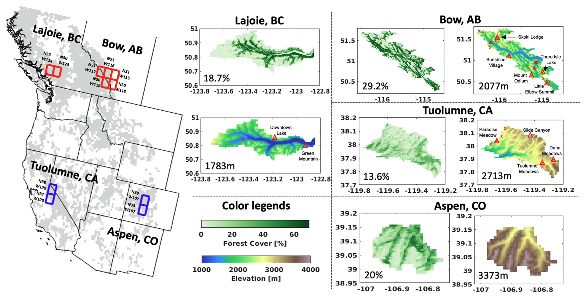
Figure 1 Location, forest cover, and elevation maps over the study domains, including the Tuolumne basin (CA) and Aspen (CO) in the WUS and the Lajoie basin (BC) and Bow River basin (AB) in western Canada. The current Snow CCI SWE mask (that excludes mountainous areas) is shown in grey in the left panel. The test tiles (1° × 1°) that include the four study domains are outlined in red (Canada) and blue (WUS) and fall almost exclusively within the Snow CCI SWE mask. Degrees N and W in the left panel correspond to the lower-left corner of each of these test tiles. The average elevation and forest cover are annotated in the spatial maps, where snow pillow locations are shown with red triangles and snow courses are shown with red crosses.

More specifically, the upper Tuolumne Basin is a high-elevation watershed in the Sierra Nevada of California (CA). The elevation ranges from approximately 1241 to 3700 m a.s.l. The precipitation is dominated by snowfall during the winter. The snowmelt during the spring and early summer fills the Tuolumne River, which is dammed at Hetch Hetchy to provide water for San Francisco. Aspen is a high-elevation domain situated in the Roaring Forking watershed in central Colorado (CO) on the western side of the Continental Divide. The elevation varies within the range of 2550 to 4100 m a.s.l. The snowmelt feeds the Castle and Maroon creeks and contributes to almost all of the water supply to the city of Aspen.

The Lajoie basin is a watershed in the Coast Mountains of British Columbia (BC). The elevation within the Lajoie basin varies from 800 to 2800 m a.s.l. The forested areas at low elevations cover 47 % of the total watershed area (Darychuk et al., 2023). The snowmelt is a critical source of downstream freshwater to Downton Lake formed by the Lajoie dam. The Bow River basin in southern Alberta (AB) is a well-studied basin located in the Canadian Rockies. The elevation spans from 1250 to 3500 m a.s.l. The snowmelt from the Bow River Basin provides around 80 % of the Bow River streamflow, which is vital for hydroelectric power, irrigation, and significant downstream populations (Wang et al., 2019). Despite the value of water resources and the frequency of damaging flood events (Pomeroy et al., 2015), there is no systematic airborne or satellite snow monitoring program for the mountain regions of western Canada.

The snow reanalysis framework is applied over tiles of 1° × 1° (latitude–longitude). The tiles that cover the application domains are outlined in the location map (Fig. 1) and are used for the reanalysis application. In this study, we conducted the Snow CCI reanalysis for water years (WYs) 2001–2019 across the study domains, corresponding to the period of available Snow CCI fSCA data.

2.3 Bayesian snow reanalysis framework

This study uses a previously developed Bayesian snow reanalysis framework (Margulis et al., 2015) to generate SWE reanalysis estimates by assimilating the Snow CCI fractional snow-covered area (fSCA). The SWE reanalysis framework has been applied to generate snow reanalyses over the Sierra Nevada (Margulis et al., 2016), the Andes (Cortés et al., 2016), High Mountain Asia (HMA) (Liu et al., 2021), and the WUS (Fang et al., 2022) using Landsat-derived fSCA. These applications of SWE reanalysis have been verified against available in situ and airborne SWE estimates.

The method combines a spatially distributed land surface model (LSM) and a particle batch smoother (PBS) to estimate snow dynamics. The LSM, specifically the simplified simple biosphere (SSiB)–snow–atmosphere–soil transfer (SAST) model (SSiB–SAST; Sun and Xue, 2001), is used to simulate SWE, snow density, and snow depth. The Liston snow depletion curve (SDC) model (Liston, 2004) is coupled with the LSM to predict fSCA based on modeled SWE and its sub-grid heterogeneity. The LSM–SDC accounts for prior uncertainties from meteorological forcing, model parameters, and sub-grid snow variability. Uncertainty models and parameters used in the LSM–SDC are described in Fang et al. (2022). In the prior step, these uncertainties are embedded in an ensemble of model estimates. Assimilation of fSCA measurements to produce posterior SWE estimates is done using a particle batch smoother (PBS) method, which involves assigning likelihood-based weights to ensemble members. The assimilation of fSCA estimates is intended to improve SWE estimates relative to the prior. The preprocessing of Snow CCI fSCA for SWE reanalysis including cloud screening (Sect. 2.3.1) and viewing geometry screening (Sect. 2.3.2) processes are carefully conducted to avoid misclassifying cloud, forests, and other non-snow features as snow.

While previous applications of the SWE reanalysis via the assimilation of Landsat fSCA (with a native resolution of 30 m and scaled up to ∼100–500 m and a measurement error of 10 %) have shown significant promise (Fang et al., 2022), herein we evaluate SWE estimates derived from the globally available Snow CCI fSCA product at 1 km resolution. We focused first on the WUS because previous well-validated implementations of the BSRF are available as the baseline. The implementation and validation over two watersheds in western Canada were performed in order to assess transferability to new regions. The Landsat reanalysis is performed in parallel to provide a baseline for the comparison.

2.3.1 Cloud screening for Snow CCI fSCA data

The depletion of fSCA through the snowmelt season is informative to constrain the SWE evolution (Margulis et al., 2019) in both accumulation and melt seasons. Therefore, the PBS approach that assimilates time series of Snow CCI fSCA over the full WY (i.e., all images at once) is used to update the prior snow estimates in a single step. In previous SWE reanalysis applications (over the WUS, Andes, and HMA), the internal cloud mask from the sensor and an ad hoc cloud fraction threshold were used to identify images with “significant” cloud cover that were screened out entirely vs. those that were included but with cloudy pixels within the image screened out. The tile-wise images with a cloud fraction greater than the threshold were deemed “too cloudy” such that they might have a significant misclassification of cloudy pixels as snowy pixels. Previously used cloud fraction thresholds were 0.4 for Landsat and 0.1 for MODIS-derived MODSCAG (Painter et al., 2009). There is a trade-off involved in using a single threshold. Opting for a higher threshold increases the pool of fSCA images, albeit with the risk of higher uncertainty such as misclassifying clouds as snow pixels. On the other hand, selecting a lower cloud threshold results in screening out more images, potentially yielding fewer informative measurements but with an enhanced overall quality. Therefore, selecting the Snow CCI cloud fraction threshold across test domains required careful consideration. Given that Snow CCI fSCA includes a unique internal cloud mask compared to other products, it is essential to derive a cloud fraction threshold specific to the Snow CCI fSCA product. The cloud mask in the Snow CCI product is derived using an adapted version of the Simple Cloud Detection Algorithm 2.0 (SCDA2.0) (Metsämäki et al., 2015), which is based on the brightness-temperature difference between 11 and 3.7 µm, with clouds exhibiting significantly large negative values.

The cloud fraction threshold was estimated through examination of the historical tile-wise cloud distributions (as diagnosed by the Snow CCI cloud mask) covering the test domains. Figure 2 shows the historical cumulative distribution functions (CDFs) (spanning WYs 2000–2019) of tile-wise cloud fraction (aggregated by domains) for each WY in dashed grey curves and for the multi-year (WYs 2000–2019) median in solid red curves. The median of the historical CDF (the intersection of the dashed blue lines) is presumed to represent a typical tile-wise level of cloudiness in the binary classification of images into cloudy and less cloudy categories. However, there is a large variation in the median cloud fraction across different tiles/domains. It is apparent that the selected tiles in the WUS (Fig. 2a and b) are less cloudy than those in western Canada (Fig. 2c and d). The CDF of the tile-wise median cloud fraction across all test tiles is shown in Fig. 2e. In order to reconcile varying tile-wise median cloud fractions and identify a single tile-independent threshold, the median value – approximately 0.6 (indicated by the red asterisk) – was selected as the cloud fraction threshold. By setting the threshold at the median, we aim to identify cloudy images while minimizing the risk of false positives (which could result in eliminating more images with a lower tile-independent threshold, although certain snowy pixels remain valuable, particularly for Canadian tiles) and false negatives (including more cloudy images that likely misclassify snow as cloud, with a higher tile-independent threshold, especially for the WUS tiles) in the cloud classification process. Therefore, Snow CCI fSCA images with an internal cloud fraction greater than 60 % are removed.

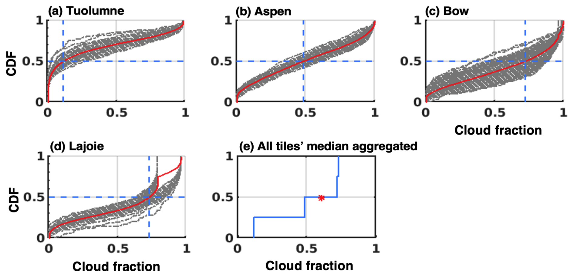
Figure 2 (a–d) CDFs of tile-wise cloud fraction (aggregated by domains) for WYs 2000–2019 derived from the internal Snow CCI cloud mask. The dashed grey curves represent the CDF of cloud fraction for each WY, and the solid red curve represents the CDF for the multi-year period (WYs 2000–2019). The intersection of dashed blue lines indicates the tile-wise median cloud fraction. (e) The CDF of the median cloud fraction for all tiles, with a red asterisk representing the cloud fraction threshold.

2.3.2 Viewing geometry effects on the fSCA assimilation

A key difference between the Snow CCI fSCA and the Landsat fSCA is the sensor viewing geometry. The 16 d Landsat repeat frequency is due to its near-nadir viewing geometry. The Snow CCI fSCA product used in this study is derived based on data from the MODIS sensor, which has a wide swath (by scanning at different angles) to provide a daily revisit frequency. As a result, some daily images can have significant off-nadir viewing angles near the edge of the swath. This effect has been shown to lead to differences due to distorted irregular pixels at large zenith angles (Dozier et al., 2008), with negative impacts on the retrieval of fSCA, especially in forested areas (Margulis et al., 2019; Rittger et al., 2020). The primary result of this is that fSCA estimates should reflect less error when derived from near-nadir viewing than those pixels at significantly off-nadir viewing. Following Margulis et al. (2019), the error covariance of fSCA measurements that penalizes the off-nadir viewing geometry angles can be represented as

$$\begin{array}{}\text{(1)}& C_v^{\text{Snow CCI}}\left(\mathit{\theta }\right)={\displaystyle \frac{C_v^{\text{Snow CCI}}(\mathit{\theta }=\mathrm{0})}{w\left(\mathit{\theta }\right)}},\end{array}$$

where the measurement error covariance $C_v^{\text{Snow CCI}}\left(\mathit{\theta }\right)$ is a function of the MODIS sensor viewing angle θ, obtained from the MOD09GA product. The numerator $C_v^{\text{Snow CCI}}(\mathit{\theta }=\mathrm{0})$ is the error covariance at nadir, and w(θ) is a specified weighting function that is associated with non-nadir scan angles (more detailed explanations are in Dozier et al., 2008):

$$\begin{array}{}\text{(2)}& w\left(\mathit{\theta }\right)={\displaystyle \frac{p^{\mathrm{2}}\cos \mathit{\theta }}{p_{\parallel }{p}_{\perp }}},\end{array}$$

where p is the linear pixel dimension at nadir and p_∥ and p_⊥ are the along-track and cross-track pixel dimensions at a non-nadir angle. The more off-nadir measurements (with more significant pixel elongation) have smaller w values and, thus, larger measurement error covariances. We recognize that increasing the measurement error covariances does not correct any bias; biases induced by off-nadir effects may still introduce systematic errors in the posterior results. While these viewing geometry corrections may screen out highly problematic forested pixels that are significantly affected by the viewing geometry, it should be noted that Eq. (3) does not explicitly incorporate the underlying forest cover as a factor (Rittger et al., 2020). Based on the assimilation of MODIS-based fSCA (Margulis et al., 2019), the error covariance at nadir (i.e., $C_v^{\text{Snow CCI}}(\mathit{\theta }=\mathrm{0})$) is specified as ∼(15 %)² for the MODIS-based Snow CCI fSCA. The relationship between the error covariance $C_v^{\text{Snow CCI}}\left(\mathit{\theta }\right)$ and w(θ) can be specified as

$$\begin{array}{}\text{(3)}& C_v^{\text{Snow CCI}}\left(\mathit{\theta }\right)={\displaystyle \frac{C_v^{\text{Snow CCI}}(\mathit{\theta }=\mathrm{0})}{w\left(\mathit{\theta }\right)}}\approx {\displaystyle \frac{(\mathrm{15}\mathit{\%}{)}^{\mathrm{2}}}{w\left(\mathit{\theta }\right)}}.\end{array}$$

Note that the weighting function w(θ) varies within (0,1] by definition. Following the screening method for the viewing geometry (Margulis et al., 2019), a threshold of w(θ) needs to be identified to exclude the measurements at pixels with significant distortions. The rationale behind selecting the threshold of w(θ) is the need to eliminate measurements with lower quality, which could potentially introduce noise or inaccuracies into the assimilation. However, there is a trade-off between the threshold of w(θ) and the number of informative fSCA measurements for assimilation. If the threshold were set too high, there is a risk of discarding a substantial number of measurements, potentially leading to a loss of valuable fSCA information during the ablation season and limiting the effectiveness of assimilation.

To determine the threshold of w(θ), we show the impact of w(θ) on the accuracy of the assimilated fSCA, where the accuracy (measurement error standard deviation) is given by $\sqrt{C_v^{\text{Snow CCI}}\left(\mathit{\theta }\right)}$, using $C_v^{\text{Snow CCI}}\left(\mathit{\theta }\right)$ from Eq. (3). A smaller $\sqrt{C_v^{\text{Snow CCI}}\left(\mathit{\theta }\right)}$ represents a more accurate Snow CCI fSCA. As shown in Fig. 3, the threshold of w(θ)∼0.2 is a reasonable number to exclude less reliable measurements (w(θ)<0.2) with a sharp increase in the uncertainty at higher viewing angles (θ>50°) that are unlikely to provide useful information in the assimilation step. As w(θ) approaches 1 (i.e., θ=0°), the measurement error approaches that of the Landsat fSCA. The measurement error in Landsat fSCA used in the Landsat reanalysis reference is indicated by the triangle (i.e., 0.1 at nadir, where w(θ)=1, θ=0°) in Fig. 3.

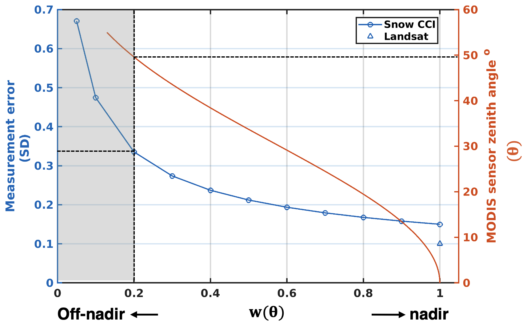
Figure 3 The left y axis shows the impact of the w(θ) threshold on the accuracy, i.e., measurement error standard deviation, of Snow CCI fSCA for assimilation. The right y axis shows the function of w(θ). Areas below the threshold of w=0.2 are excluded from the assimilation. The measurement error in Landsat fSCA is represented by the triangle (i.e., 0.1 at nadir).

Figure 4 summarizes the screening process for Snow CCI fSCA as described in Sects. 2.3.1 and 2.3.2. Figure 4a–c illustrate an example of the cloud screening with the threshold of 60 % for the Snow CCI fSCA images. In Fig. 4a, all data within the scene are discarded because the tile-average cloud fraction (76.5 %) exceeds 60 %, a threshold hypothesized to increase the likelihood of misclassifying cloud as snow. For the remaining images (e.g., Fig. 4b and c), pixel-wise clouds are removed using the internal Snow CCI cloud mask before assimilation. The remaining data are then screened for viewing geometry. The pixel-elongation effect caused by off-nadir viewing geometry is illustrated by Fig. 4c, where the horizontal stretching pattern is clearly evident. We exclude these erroneous pixels by removing Snow CCI fSCA measurements with a pixel-wise w(θ) of less than 0.2 as illustrated in Fig. 4d–f.

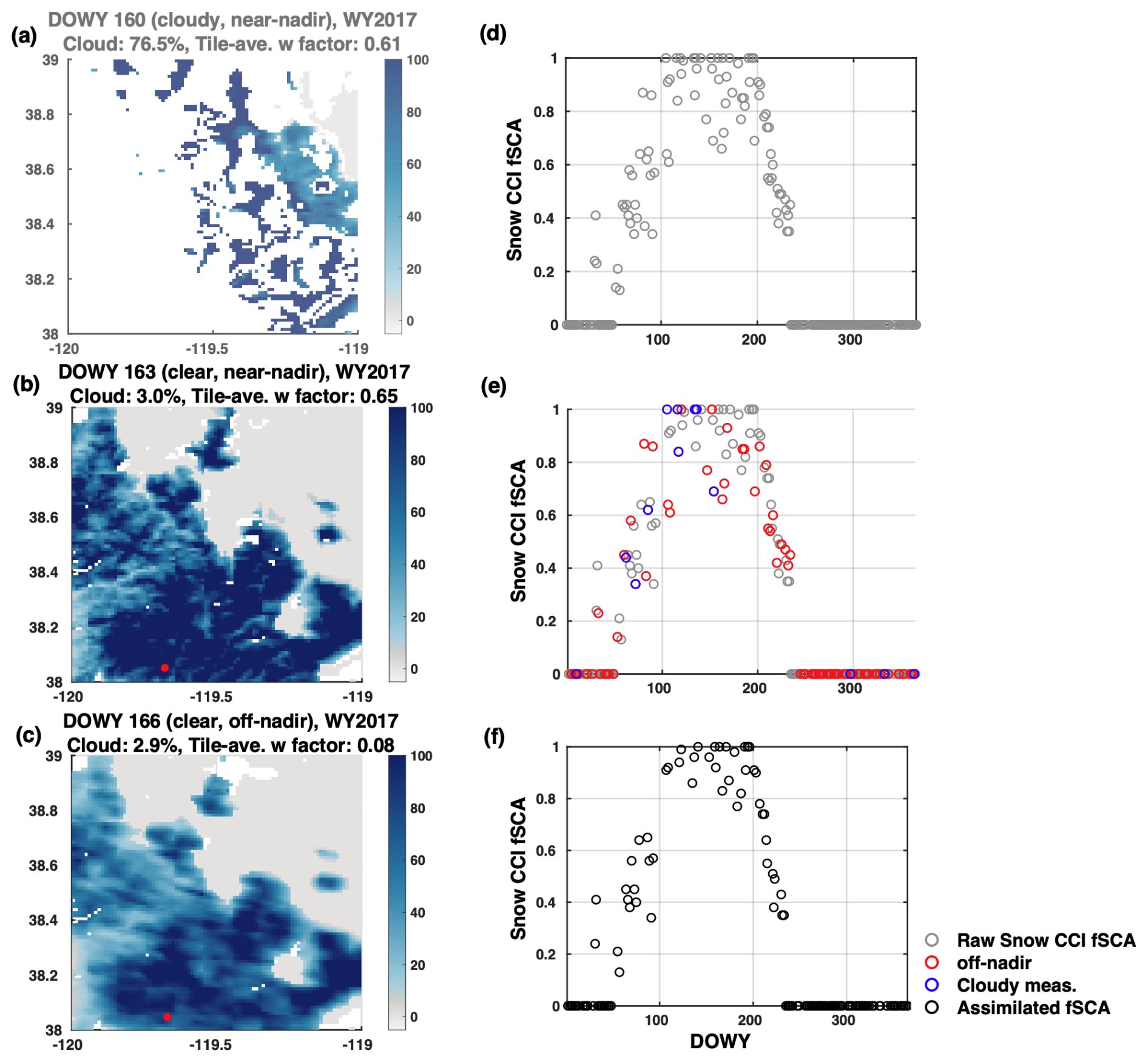
Figure 4 Illustration of cloud and off-nadir screening processes. DOWY means the day of the water year. Panels (a–c) display the cloud screening of raw Snow CCI fSCA images. The white color represents clouds, and the grey color represents fSCA lower than 10 %. Panel (a) is discarded completely due to cloud coverage above 60 %. Panel (b) has a domain-wide cloud fraction below the threshold, so only cloudy pixels are screened out. Panel (c) displays an off-nadir image on a clear day. Off-nadir measurements from panel (c) are excluded in the (e) pixel-wise screening. Panels (d–f) present the complete screening process of Snow CCI fSCA at a sample pixel (indicated by a red dot on the left panel). The daily time series of Snow CCI fSCA show (d) raw data, (e) data to be removed through pixel-wise cloud screening and off-nadir screening, and (f) data to be assimilated.

Not all the assimilated fSCA data contribute to the posterior SWE estimate as illustrated in Fig. 5, which displays the basin-average number of assimilated fSCA measurements per year for both Snow CCI and Landsat and specifically those that are informative. The informative fSCA measurements are those that contribute to the posterior update and can be identified as those that occur when the prior ensemble fSCA spread is greater than zero (most often during the ablation season). Additionally, the spatiotemporally averaged measurement error for each case is depicted by the circle that is projected onto the right y axis of Fig. 5. The Landsat error is fixed at 10 %, while Snow CCI is 15 % at a minimum but is closer to 20 % when the viewing geometry is also considered. It is evident that Landsat provides more accurate fSCA measurements with a lower measurement error at a lower repeat frequency, whereas Snow CCI generally has a higher number of informative fSCA measurements but with higher measurement errors.

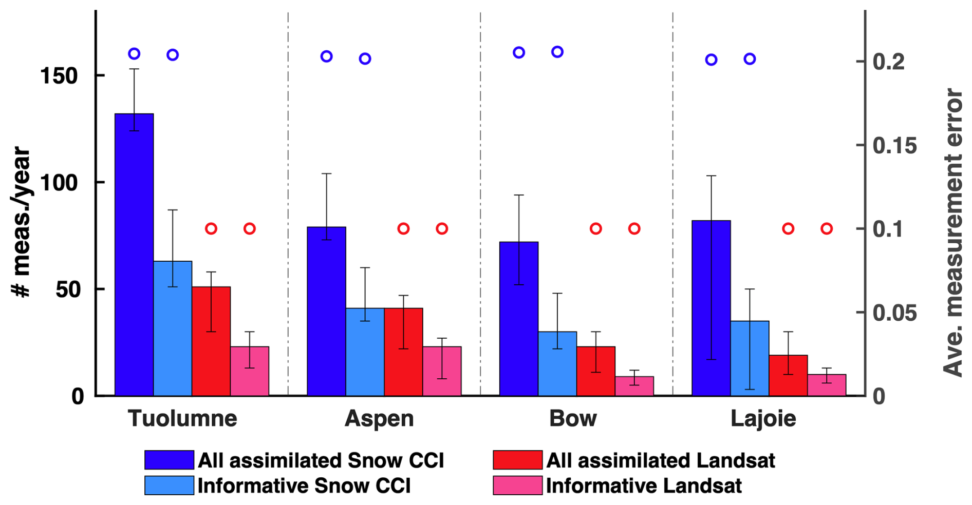
Figure 5 The left axis shows a boxplot of the domain-average number of all assimilated and informative Snow CCI fSCA and Landsat fSCA measurements per year. Informative fSCA measurements are those that contribute to the posterior update, which only occurs when the prior ensemble spread of fSCA is greater than zero. The right axis shows the spatiotemporally averaged measurement error for Snow CCI (in blue circles) and Landsat (in red circles).

2.4 Evaluation data and methods

2.4.1 Verification with independent datasets

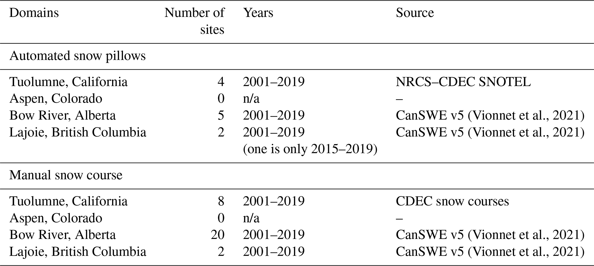
The performance of the Snow CCI reanalysis estimates is evaluated through comparisons with independent in situ observations from automated snow pillows and manual snow courses as well as airborne lidar-based SWE estimates for the WUS. Each type of reference data has its strengths and weaknesses. Snow pillows (Beaumont, 1965) provide daily or even hourly SWE estimates for a ∼10 m² area, which may not be spatially representative at the 1 km² grid scale (Herbert et al., 2024; Meromy et al., 2013). However, the high temporal frequency provided by automated snow pillows is helpful in capturing the seasonal evolution of SWE, important within the BSRF framework which relies on a snow depletion curve (Liston, 2004). Snow courses provide monthly and/or biweekly SWE measurements. The measurements are averaged along a ∼100–500 m long transect. It is expected that there are discrepancies between the snow pillows and courses, even if they are collocated, unless the underlying SWE is spatially homogeneous. Despite the representativeness issue when comparing the in situ measurements to 1 km² gridded estimates and sampling a very small fraction of the test domains, we perform the verification in terms of the annual peak SWE and the temporal correlation of daily SWE, where the correlation is insensitive to biases. Airborne lidar data provide spatially complete measurements of SD or estimates of SWE but are available only for specific dates, typically near peak SWE. Estimates of snow density are needed to go from SD to SWE (Painter et al., 2016).

In situ SWE measurements are available from the Natural Resources Conservation Service (NRCS) and the California Data Exchange Center (CDEC) via https://wcc.sc.egov.usda.gov/reportGenerator/ (last access: 13 May 2025) for the WUS, and for Canadian domains, access is provided through the Canadian historical Snow Water Equivalent (CanSWE) dataset (Vionnet et al., 2021). Table 1 summarizes the number of in situ sites and years for each domain. SWE measurements are not available in the Aspen domain, and so only comparison with airborne lidar estimates is possible over that domain.

Table 1 Number of in situ sites, site years, and sources of SWE measurements used in this study. SNOTEL: SNOwpack TELemetry Network. n/a: not applicable.

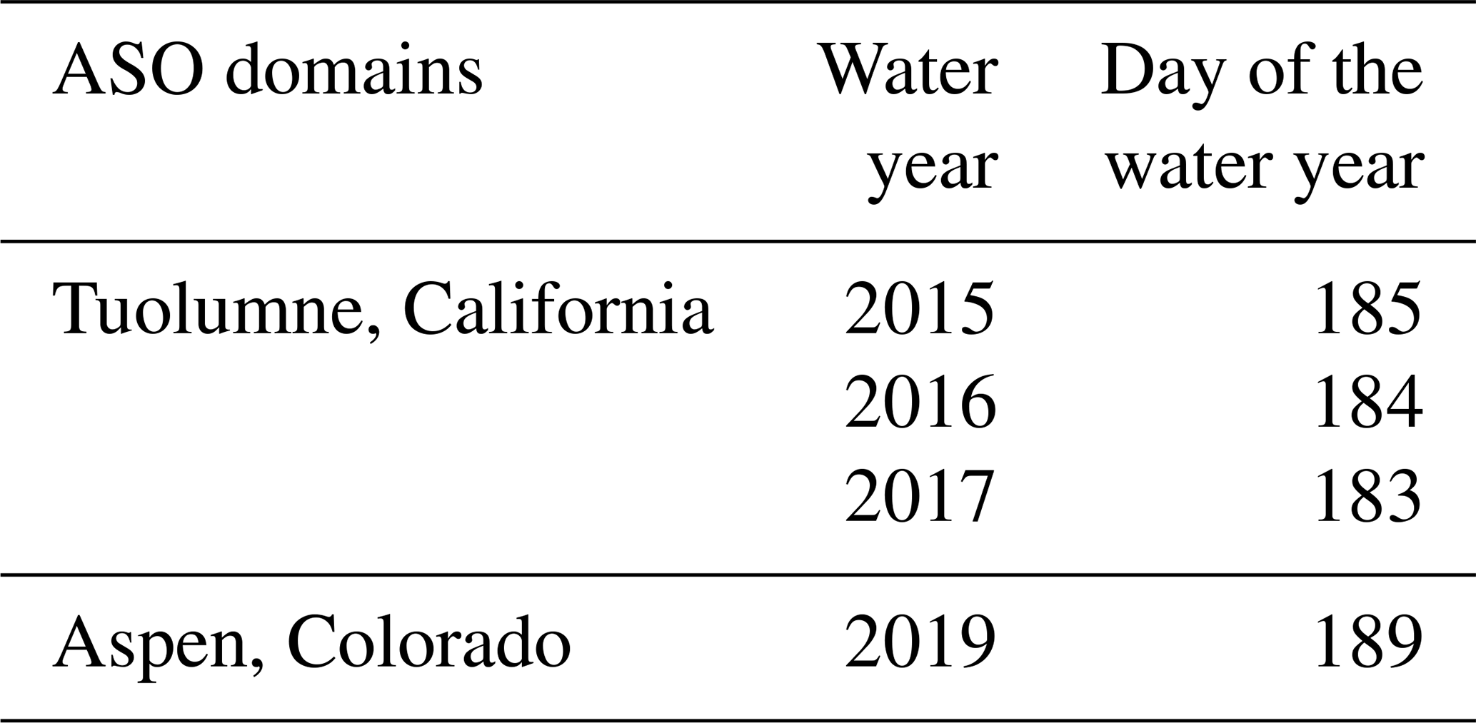
The lidar-based Airborne Snow Observatory (ASO) SWE estimates available at 50 m spatial resolution over domains in the WUS are interpolated and aggregated to the Snow CCI SWE reanalysis resolution (0.01°) for the comparison. The ASO SWE estimates closest to 1 April are only available for the WUS domains in recent years (Table 2). The following evaluation compares SWE values for these ASO measurement times shown in Table 2. Additional evaluations for other ASO times are included in Table S1 in the Supplement.

Table 2 Lidar-based measurement days closest to 1 April over study domains in the WUS (for SWE).

2.4.2 Comparison with the Landsat SWE reanalysis dataset

In the absence of spatiotemporally continuous reference SWE, we use a SWE reanalysis dataset produced by assimilating cloud-free Landsat fSCA aggregated to a spatial resolution of 0.01° (∼1 km). This dataset is developed using the same method, which was produced for the WUS at a spatial resolution of ∼500 m (16 arcsec) for 1985–2021 (Fang et al., 2022). The specific thresholds, uncertainty parameters, etc. are described in Fang et al. (2022) (Table 3). The performance of the Landsat reanalysis SWE is well understood over the WUS but not over western Canada, as it has not been produced there previously. We consider the performance of the Landsat and Snow CCI reanalysis SWE against the independent reference data and relative to each other. Such comparisons allow us to diagnose the performance of the Snow CCI reanalysis and understand to what extent the Snow CCI fSCA can be used for the SWE reanalysis.

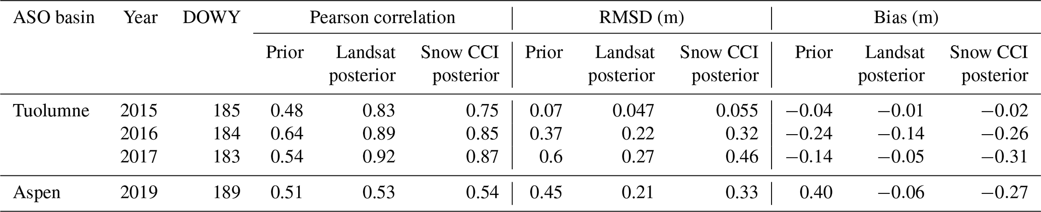
Table 3 SWE comparison statistics between ASO SWE estimates against prior and posterior snow reanalysis SWE on ASO measurement days (day of the water year, DOWY) closest to 1 April.

3 Results and discussion

In this section, we first evaluate the performance of the reanalysis framework adapted from using Landsat fSCA to Snow CCI MODIS fSCA inputs within the well-validated WUS domains. By comparing with the previously validated Landsat reanalysis reference, we can analyze the impact of differences in fSCA datasets on the accuracy of the SWE estimation. Subsequently, we extend the study regions to the western Canadian domains, which are more forested and located at higher latitudes than the WUS (Fig. 1). The reanalysis framework has not been applied to the western Canadian domains yet, and the performance has not been previously verified.

3.1 Application over previously studied WUS domains

3.1.1 Verification against in situ SWE measurements

Posterior peak SWE estimates from both the Snow CCI reanalysis and Landsat reanalysis are compared with in situ measurements (snow pillows and courses) available in the Tuolumne watershed. In general, the Landsat reanalysis performs better than the Snow CCI reanalysis with a Pearson correlation of 0.91 and root mean square deviation (RMSD) of 0.26 m, compared to a Pearson correlation of 0.47 and RMSD of 0.53 m. The scatterplot in Fig. 6 presents the comparison of the in situ peak SWE against collocated posterior peak SWE estimated from the Snow CCI reanalysis. To incorporate the Landsat posterior SWE estimates into this comparison, we use different colors to represent absolute relative differences in basin-average peak SWE estimated from Snow CCI relative to Landsat. These values are computed as absolute differences in basin-average peak SWE, normalized by basin-average peak SWE from the Landsat reference. Lower values of absolute relative differences indicate years when Snow CCI posterior SWE is more similar to Landsat posterior SWE on a basin scale and vice versa. For example, the Snow CCI estimates closely match the in situ measurements when the absolute relative differences are within the range of 0–0.1 (in red). Conversely, the estimates are more scattered when the Snow CCI estimates diverge significantly from the Landsat reference (e.g., greater than 0.5 in grey). The right panel in Fig. 6 displays the statistics (i.e., correlation and RMSD) of the verification against in situ peak SWE. The statistics are computed for each range bin, using data points represented in different colors. The Snow CCI reanalysis performs well in years when the basin-average peak SWE better matches the Landsat reference and the relative differences are lower than 0.3. In such cases, correlation values are greater than 0.8 and the RMSD are lower than 0.5 m. However, other years with divergence in basin-average peak SWE between Snow CCI and Landsat exhibit lower correlation and higher RMSD values relative to the in situ measurements. The reason for discrepancies between Landsat- and Snow CCI-derived SWE is discussed below in Sect. 3.1.3.

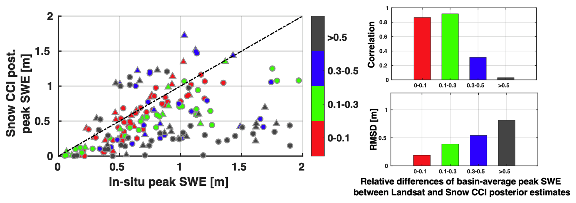
Figure 6 Scatterplot of Snow CCI posterior peak SWE vs. in situ peak SWE at snow pillow sites (triangles) and snow course sites (circles) in the Tuolumne domain. The color represents the unitless relative differences in basin-average peak SWE relative to the Landsat posterior SWE reference. Bar plots show variations in the Pearson correlation and RMSD with in situ measurements across different ranges of relative peak SWE differences relative to the Landsat reference.

Figure 7 displays the temporal (daily) SWE comparison for pixels containing snow pillows in the Tuolumne domain. The locations of snow pillow sites are shown in Fig. 1. The correlation square is computed by comparing Snow CCI and Landsat posterior daily SWE against in situ daily SWE greater than 1 cm. In the Tuolumne domain, posterior daily SWE at snow pillow pixels have high correlations against in situ SWE. The average R² values are 0.85 and 0.92 for the Snow CCI and Landsat reanalysis, respectively. The bottom panel depicts differences in the R² relative to the prior daily SWE comparison. Specifically, cases in blue colors and highlighted by the black boxes represent site years where the reanalysis improves the correlation of daily SWE. For the Snow CCI reanalysis, 30 out of 59 site years show improvements in the R², while the assimilation of Landsat fSCA improves the R² for 48 out of 59 site years. For some years where there is degradation in the correlation after assimilating Snow CCI fSCA, such as 2003, 2006, 2011, and 2019, Snow CCI fSCA is likely negatively biased over the domain during the ablation season (Fig. 10). Such biases in fSCA could cause significant shifts in the time of peak SWE and the snowmelt season, which degrade the correlation of the daily SWE compared to in situ measurements.

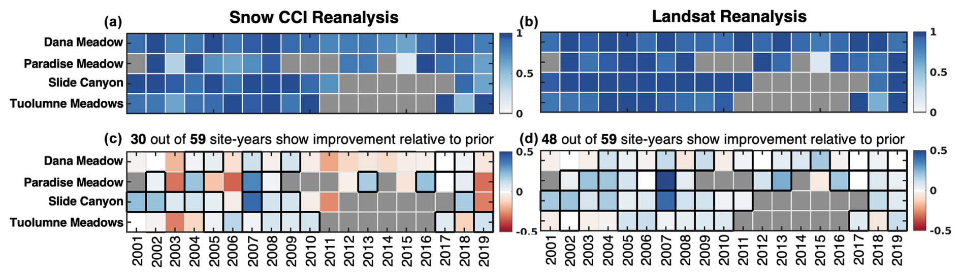
Figure 7 Temporal correlation square (R²) of (a) Snow CCI and (b) Landsat posterior daily SWE vs. snow pillow daily SWE measurements at snow pillow pixels in the Tuolumne domain. Panels (c–d) display differences between the posterior correlation and the prior correlation (posterior R² − prior R²). Station years with improvements are in the black boxes. Cases where snow pillow measurements are incomplete and/or annual peak SWE values were lower than 2 cm are greyed out.

3.1.2 Verification against ASO SWE

For the Tuolumne domain, the assimilation of Snow CCI fSCA significantly improves the correlation relative to the prior SWE on the days near 1 April compared to the ASO SWE (Table 3). The posterior Snow CCI SWE is highly correlated with ASO SWE, with correlation values ranging from 0.75 to 0.87, while the prior correlation values range from 0.48 to 0.54. The most significant improvement in the correlation occurs in WY 2017 (Fig. 8), where the RMSD decreases from 0.6 to 0.46 m. The assimilation of the aggregated Landsat fSCA shows a larger improvement in all WYs in terms of the correlation and RMSD (Table 3). The posterior Landsat SWE exhibits high correlation values ranging from 0.83 to 0.92, comparable to the statistics in previous work (refer to Table 6 in Fang et al., 2022). Evaluations with ASO surveys outside of peak SWE (Table S1) have performance consistent with those from near 1 April. Figure 8 shows that in Tuolumne, the prior SWE has positive biases over lower SWE areas at lower elevations and negative biases over higher SWE areas at higher elevations. After assimilating the aggregated Landsat fSCA, the systematic errors are reduced, with random errors more dispersed across the domain. When assimilating Snow CCI fSCA, negative biases exist in posterior SWE across most of the domain.

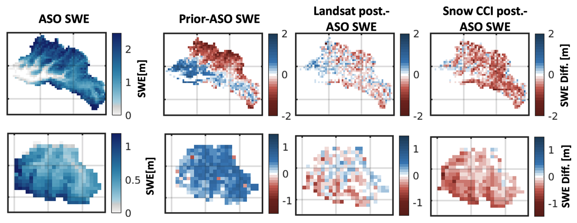
Figure 8 Comparison of ASO SWE with prior and posterior SWE at WUS ASO sites: Tuolumne basin on 1 April of WY 2017 and Aspen on 8 April of WY 2019.

For the Aspen domain (Table 3), the correlation of the posterior SWE in WY 2019 is comparable to the value of the prior SWE, while the RMSD decreases from 0.45 to 0.33 m (for Snow CCI) and 0.21 m (for Landsat). The correlation values are lower than the values seen in the Tuolumne domain. This could be because the snow albedo uncertainty is not well characterized in Colorado (Fang et al., 2022), where studies have shown that snow albedo is influenced by factors such as dust, black carbon, and other light-absorbing particles (Deems et al., 2013). The spatial map (Fig. 8) shows that the prior SWE is higher than the ASO SWE across Aspen. The assimilation of remotely sensed fSCA lowers the SWE estimates, with Snow CCI exhibiting more negative biases than the Landsat reference.

3.1.3 Comparison to Landsat-based reanalysis

Contributing factors to fSCA differences

The performance of SWE reanalysis over mountain areas is primarily affected by the accuracy of the assimilated fSCA and the prior estimates. Since the prior estimates are identical for the Landsat and Snow CCI reanalysis, any differences in the posterior are due to fSCA. The annual and interannual comparison of fSCA observations from Snow CCI against Landsat provide insight into the impact of fSCA differences on the accuracy of SWE estimation.

A key difference between the two fSCA products is resolution: the raw nadir resolution of Landsat (∼30 m) is significantly higher than that of MODIS (∼500 m), which can improve its ability to resolve spatial patterns and see through forest gaps. Snow CCI tends to underestimate fSCA in forested areas (Fig. S1 in the Supplement). Additionally, the broader range of viewing angles observed by the MODIS sensor has a “smearing” effect that elongates pixels when viewed at higher zenith angles (Dozier et al., 2008; Fig. 5). Beyond considerations of resolution and viewing angle, different retrieval algorithms are used to derive Snow CCI and Landsat fSCA, which can lead to both systematic (biased) and random differences. Images of Landsat fSCA used in this study are retrieved via a spectral end-member unmixing approach (Cortés et al., 2014). Snow CCI fSCA images are derived using the SCAmod algorithm (Metsämäki et al., 2012, 2015), a semi-empirical method retrieving fSCA using observed reflectance with predetermined parameters. Recognized issues associated with SCAmod include the upper/lower bounds of fSCA, which can exceed 0–1 when the observed reflectance is higher/lower than the limits allowed by the semi-empirical model (Metsämäki et al., 2015). Although Snow CCI fSCA constrains the bounds to 0–1, biases could exist when the retrieved fSCA is near the bounds. For example, Snow CCI fSCA tends to overestimate Landsat fSCA over bare soil areas with fSCA values near 100 % (Fig. S1). The SCAmod algorithm also applies a temperature threshold of 288 K to mitigate the misclassification of snow cover caused by reflective non-snow targets. This temperature threshold has a tendency to remove low fSCA values (Riggs and Hall, 2012). Snow CCI fSCA tends to be underestimated compared to Landsat fSCA during the late ablation season when snow cover depletes (Fig. S1).

Long-term SWE climatology

The spatial pattern of climatological peak SWE from the Snow CCI reanalysis is similar to the Landsat-based reference with correlation values of 0.89 and 0.86 for Tuolumne and Aspen, respectively (Table 4). Both spatial maps of peak SWE and time series of the seasonal cycle (Fig. 9) show that Snow CCI underestimates SWE over the Tuolumne domain and is closer to the Landsat reference over Aspen. The mean difference in peak SWE is −0.16 m for Tuolumne and −0.03 m for Aspen, while the corresponding RMSD is 0.21 and 0.1 m (Table 4). The impact of forest cover and aspect on the accuracy of Snow CCI SWE estimates is illustrated in Fig. 9c. In both domains, the relative difference in posterior SWE increases with the forest cover fraction. This is likely because the Snow CCI fSCA has a coarser spatial resolution and cannot see through tree gaps within forested pixels as well as Landsat can. Additionally, the relative difference in posterior SWE is more negative in areas facing north and less negative (even positive) in areas facing south/east in both domains. South-facing slopes tend to receive more shortwave radiation, leading to more reflectance compared to the north-facing slopes. Note that Snow CCI fSCA is retrieved based on the SCAmod algorithm, which uses the observed reflectance data along with predetermined reflectances of snow, snow-free ground, and forest canopy via a semi-empirical reflectance-model-based method (Metsämäki et al., 2015). It is possible that the prevailing snow reflectance on south-facing slopes is higher than that applied in the SCAmod algorithm, resulting in higher values of Snow CCI fSCA than Landsat (Metsämäki et al., 2015). This result highlights a need for further work on the fSCA retrieval algorithm in relation to terrain aspect.

Table 4 Comparison statistics for the spatial maps of 19-year median peak SWE between Snow CCI and Landsat posterior estimates.

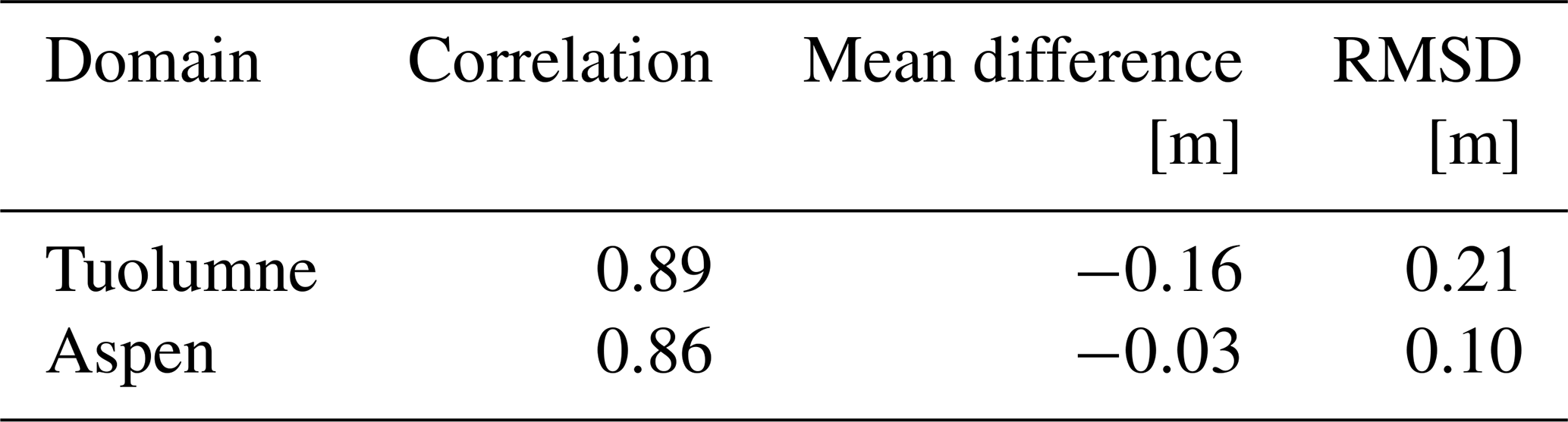
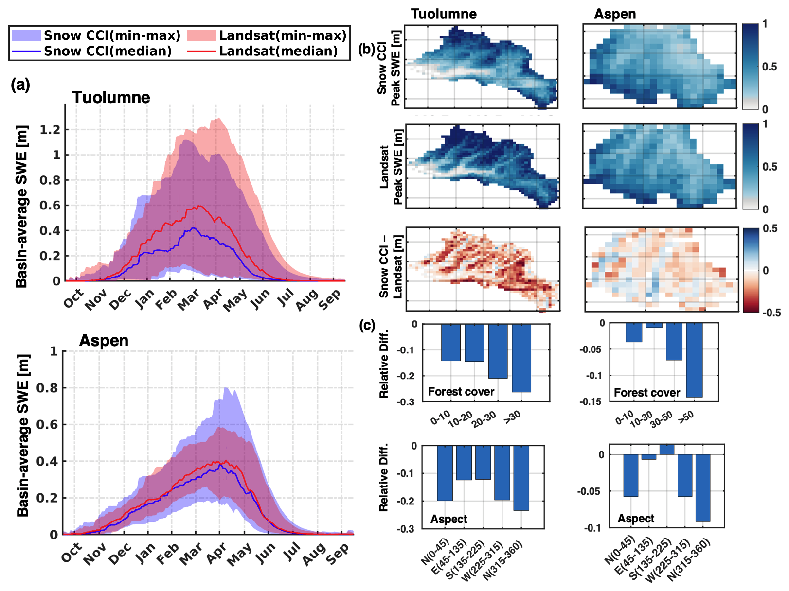
Figure 9 (a) Average seasonal cycle of basin-average posterior SWE from WY 2001 to WY 2019. The 19-year averages are displayed in solid lines, while the shaded regions represent the full range across WYs. (b) Spatial maps of the 19-year peak SWE and differences relative to the Landsat estimate. (c) Bar plots of relative differences (i.e., $(\text{Snow CCI}-\text{Landsat})/\text{Landsat}$) as functions of forest cover and aspect.

Interannual variability in SWE

The interannual variability in Snow CCI posterior SWE is similar to the Landsat-based estimates in most WYs on the basin-average scale (Fig. 10a). The basin-average differences in Snow CCI posterior fSCA estimates compared to the Landsat reference are averaged for each month from February–September (Fig. 10b displays the Tuolumne and Aspen domains as examples). The differences in the basin-average peak SWE for all WYs are significantly correlated with the average fSCA differences during the ablation season across both domains, indicated by a correlation of 0.93 (Fig. 10c). The snowmelt timing suggested by fSCA datasets also influences the accuracy of SWE estimation. The differences in the fSCA melt-out month are correlated with the differences in peak SWE by R=0.97 (Fig. 10c).

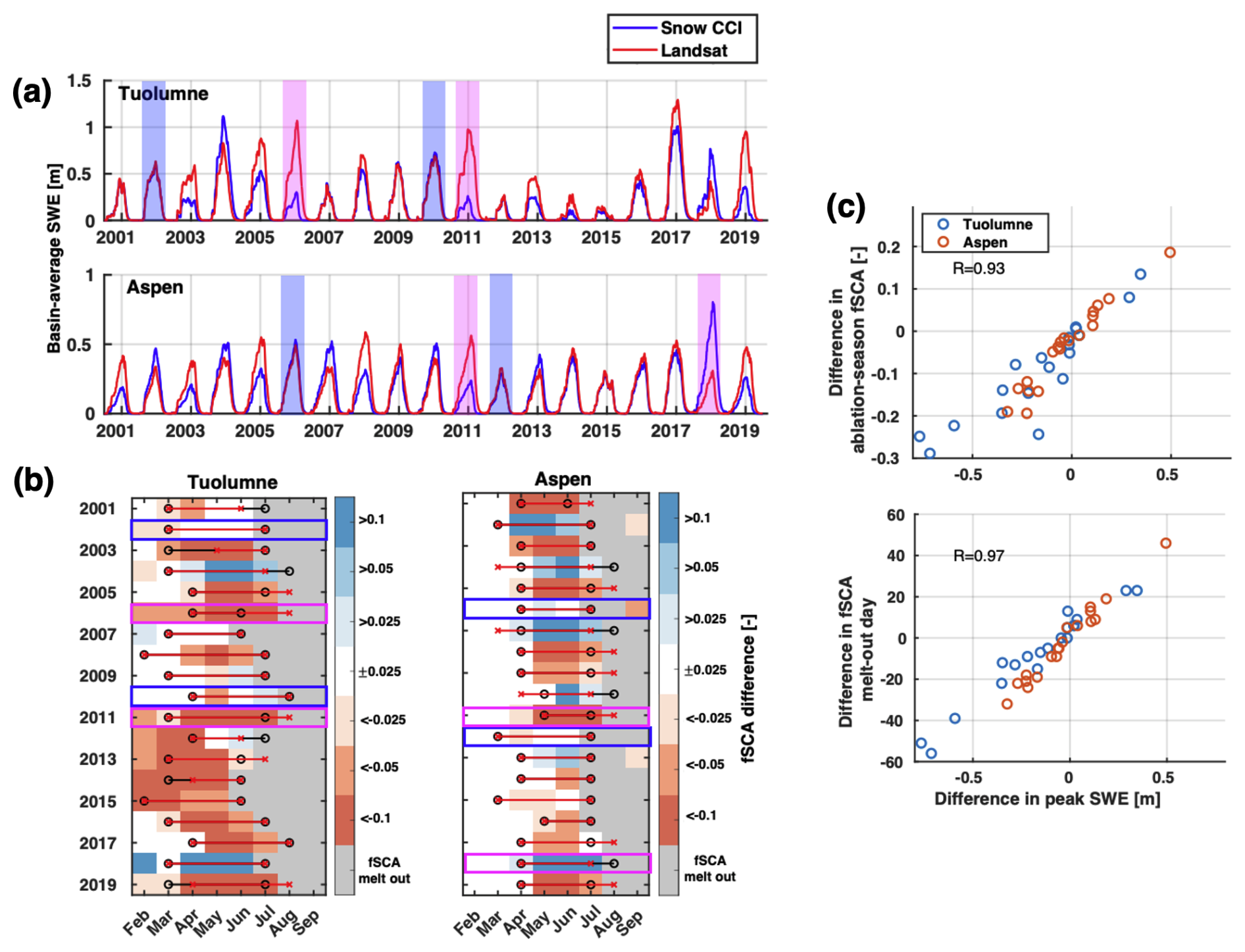
Figure 10 (a) Daily time series of basin-average posterior SWE from the Snow CCI and Landsat reanalysis. Cases of consistent performance vs. inconsistent performance between the two reanalyses are highlighted in blue and magenta, respectively. (b) Monthly basin-average posterior fSCA differences (i.e., Snow CCI fSCA − Landsat fSCA). Months when both datasets indicate snow cover melt-out are greyed out. The black circles indicate the snowmelt season estimated from the Snow CCI reanalysis (peak SWE time and the time of fSCA melt-out), and the red crosses represent the snowmelt season from the Landsat reanalysis. (c) Scatterplots of differences in peak SWE vs. mean differences in the ablation-season fSCA and vs. differences in the fSCA melt-out day.

For illustration purposes, two sample WYs with comparable performance are highlighted with blue boxes (i.e., 2002 and 2010 for Tuolumne and 2006 and 2012 for Aspen), while two typical WYs of differing performance are highlighted with magenta boxes (i.e., 2006 and 2011 for Tuolumne and 2011 and 2018 for Aspen). The fSCA values during the ablation season and snowmelt timing estimated from the Snow CCI reanalysis match the Landsat-based estimates for the comparable WYs. In contrast, significant biases exist in the snowmelt duration and fSCA values for WYs in blue boxes. In the Aspen domain, peak SWE generally occurs in April, with February and March receiving substantial snowfall. While the seasonal cycle of SWE is comparable to the Landsat reference (Fig. 9a), WY 2018 is a case of poor performance but with significant positive biases in posterior SWE. Correspondingly, Snow CCI predicts an abnormally long snowmelt season (April–September) characterized by significant positive biases in fSCA compared to the Landsat reference, particularly before July (Fig. 10b). This is a unique case where Snow CCI exhibits low-quality (biased) estimates in the Aspen domain, and the specified measurement error cannot correct biases in fSCA. Future efforts to better understand the unique behavior observed in the Aspen domain, which could help inform future algorithm development, are warranted.

The interannual differences in the basin-average posterior SWE are also associated with the number of high-quality fSCA measurements in the ablation season. Due to the limited number of coincident days when both Snow CCI and Landsat fSCA are available, the quality of the Snow CCI fSCA at each pixel is identified through a comparison with the posterior fSCA curve constrained by the Landsat fSCA. The Snow CCI fSCA measurements that are more than ±0.15 (i.e., the measurement error in Snow CCI fSCA at the nadir angle) from the Landsat posterior fSCA curve are excluded. The number of Snow CCI fSCA measurements varies across the years, as does the basin-average ratio of the number of high-quality measurements vs. the total number of measurements in the ablation season (Fig. 11). This ratio is negatively correlated with the absolute relative difference in basin-average peak SWE compared to the Landsat reference. In general, biases in the basin-average peak SWE tend to decrease as the availability of good-quality Snow CCI fSCA data in the ablation season increases. This relationship is significant for the Tuolumne domain (correlation of −0.61) but less significant for the Aspen domain (correlation of −0.28, −0.32 when the anomalous WY 2018 is excluded). In sample cases of good performance (as illustrated in Fig. 10), the fraction of good-quality Snow CCI fSCA measurements is typically higher than 0.4, whereas the sample cases of poor performance have a fraction as low as 0.2. The abnormal WY 2018 in the Aspen domain, highlighted by the grey circle in the scatterplot, is characterized by fewer than 30 % of all fSCA measurements being good quality (Fig. 11) and by significant positive biases in Snow CCI fSCA during the ablation season (Fig. 10). Together, these factors contribute to a significant relative difference (>1.5) in the basin-wide peak SWE compared to Landsat. This analysis demonstrates the challenges and limitations of defining and implementing a single global threshold. Further, it suggests there is scope to further refine the thresholds for cloudiness and the sensor viewing angle, for example by developing regionally varying thresholds, to increase the quality of Snow CCI fSCA measurements being assimilated.

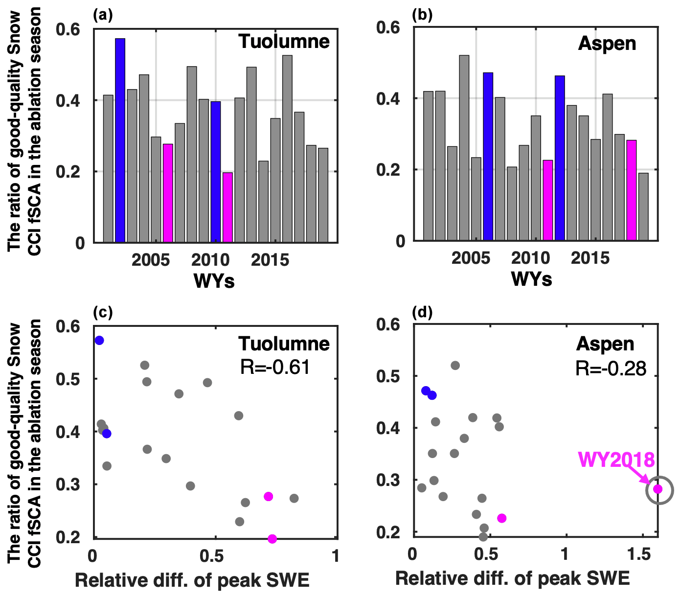
Figure 11 (a, b) Bar plots of the ratio of high-quality Snow CCI fSCA in the ablation season relative to Landsat fSCA. (c, d) Scatterplots of the ratio of high-quality Snow CCI fSCA in the ablation season vs. relative differences in basin-average peak SWE. Cases of good performance vs. poor performance are highlighted in blue and magenta, respectively, as illustrated in Fig. 10.

3.2 Application over the western Canadian domains

3.2.1 Verification against in situ SWE measurements

The performance of the Snow CCI reanalysis is evaluated through the comparison of peak SWE against in situ sites in the Bow and Lajoie domains. The Landsat reference is validated in parallel since, unlike the WUS example, the SWE reanalysis has not been applied to Canadian domains in previous work. Table 5 summarizes the statistics of the comparison of peak SWE against in situ measurements for both the Snow CCI and Landsat reanalysis. The Landsat reference performs well in both basins, with high correlation values of 0.61 and 0.75 and a low RMSD of 0.2 and 0.21 m for Bow and Lajoie, respectively. We acknowledge that the number of site years is limited in the Lajoie domain and the verification is constrained to only part of the domains. The posterior SWE estimates from the Landsat reference have better accuracy than the Snow CCI reanalysis in both domains relative to available in situ measurements. Therefore, similar to the WUS basins, the Landsat reanalysis will serve as a comparison reference.

Table 5 Comparison statistics for the 19-year peak SWE between reanalysis posterior estimates and in situ measurements.

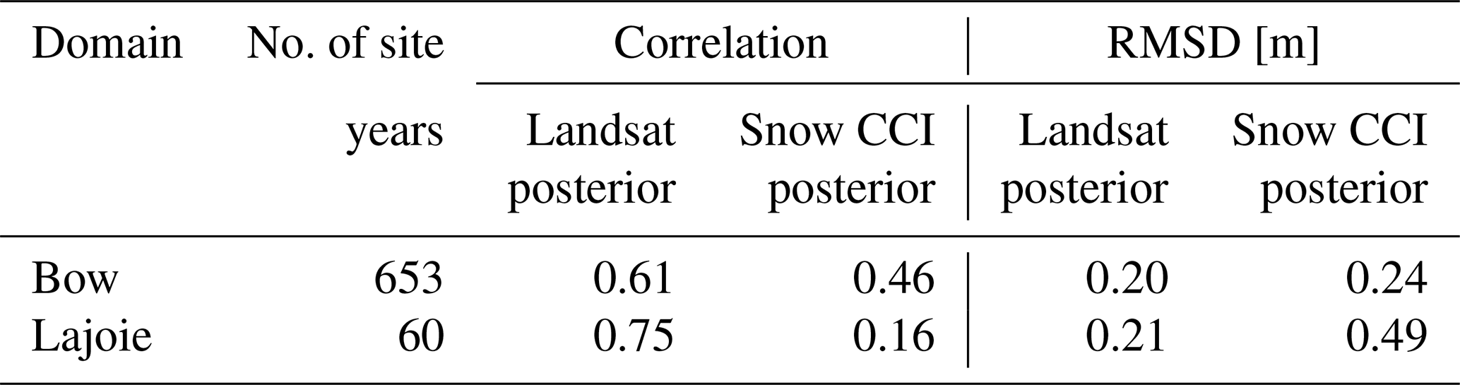
Figure 12 displays the comparison of Snow CCI posterior peak SWE against in situ peak SWE, where the colors represent the relative differences in basin-average peak SWE compared to the Landsat reference. For both domains, the correlation between posterior Snow CCI peak SWE and in situ peak SWE can be as high as 0.6 for the relative difference bin of 0–0.2 and can be as low as 0.4 and negative for the relative difference bin of >0.4. The RMSD in the peak SWE is higher when the basin-wide relative differences are larger at the basin scale. For the Lajoie domain, the number of snow pillows and snow courses is limited. The performance of the Snow CCI reanalysis is especially poor at the low-elevation densely forested Green Mountain site (Fig. 12, transparent colors), where Snow CCI SWE estimates are significantly lower than in situ SWE, which significantly degrades the statistics.

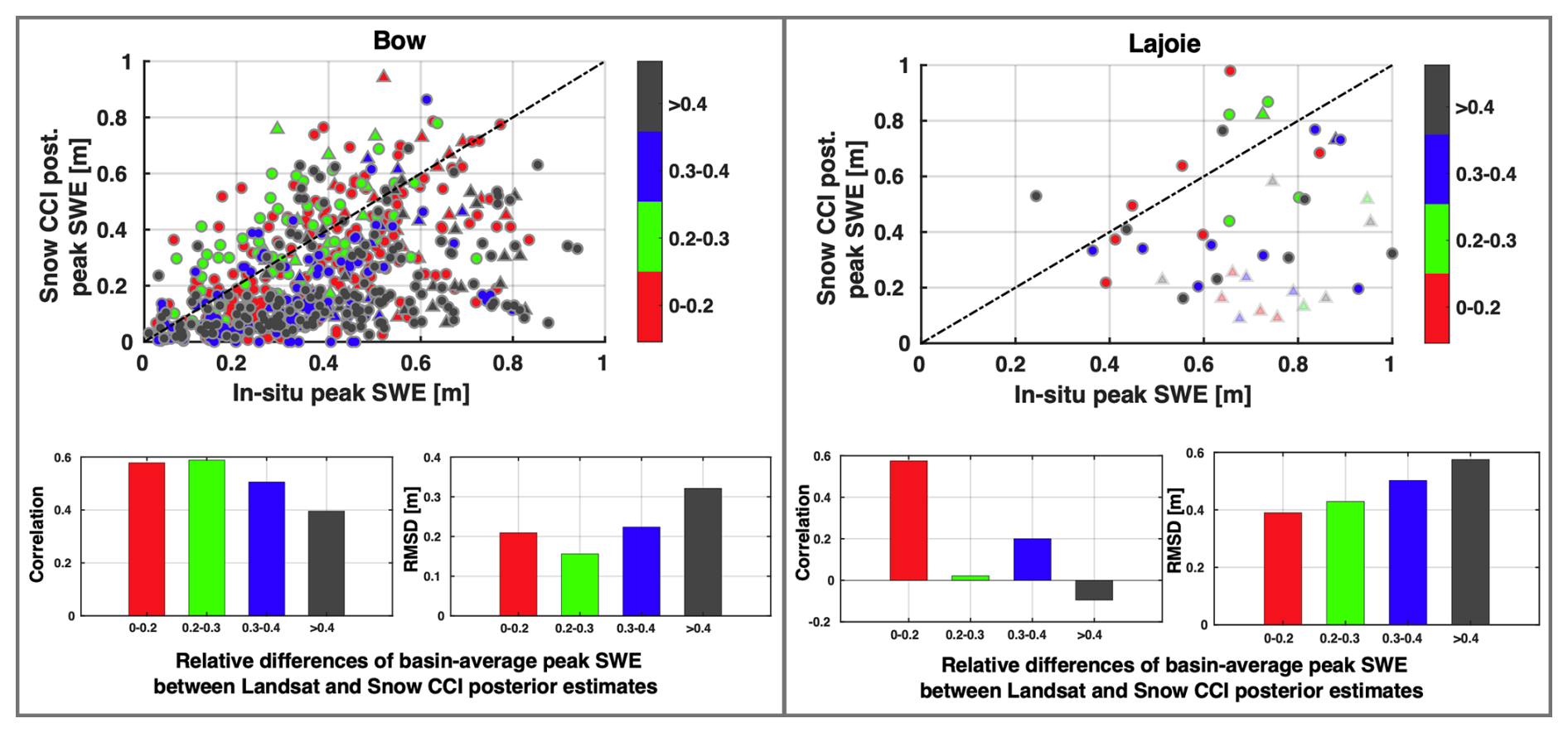
Figure 12 Same as Fig. 6 but for the Bow and Lajoie domains. Transparent colors for the Lajoie domain indicate the performance at the Green Mountain site described in the text.

The temporal (daily) SWE comparison (similar to Sect. 3.1.1) is performed for snow pillow pixels in the Bow and Lajoie domains over all WYs (Fig. 13). The average R² between in situ and posterior daily SWE is 0.85 and 0.89 for Snow CCI and Landsat, respectively. The temporal (daily) R² is much stronger than that of peak SWE. This is likely due to the strong seasonal cycle of SWE and the fact that the temporal comparison is unaffected by systematic biases. The assimilation of Snow CCI fSCA (Landsat) improves the R² values in 61 (69) out of 109 site years compared to the R² of prior estimates.

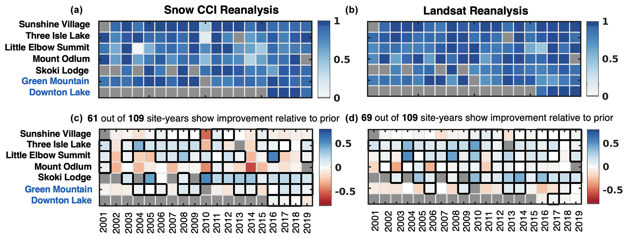
Figure 13 Same as Fig. 7 but for the Bow and Lajoie domains with snow pillow names in black and blue, respectively.

Typical fSCA and SWE time series at sample in situ sites in the Bow and Lajoie domains are displayed in Fig. S2. In selected samples, Snow CCI fSCA is generally lower than Landsat fSCA at the densely forested site (Mount Odlum), leading to an earlier snowmelt and lower SWE compared to both snow pillow measurements and Landsat reanalysis estimates. In contrast, Snow CCI fSCA is saturated and higher than Landsat fSCA at the bare soil site (Downton Lake), resulting in higher SWE and a later snowmelt season. Nevertheless, Snow CCI fSCA can provide benefits when the availability of Landsat fSCA is limited at the moderately forested site (Sunshine Village).

3.2.2 Landsat comparison

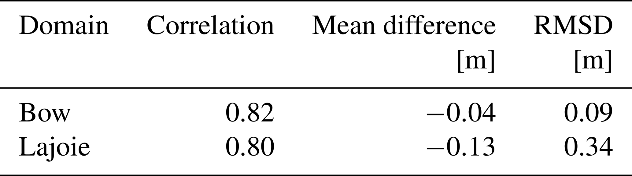
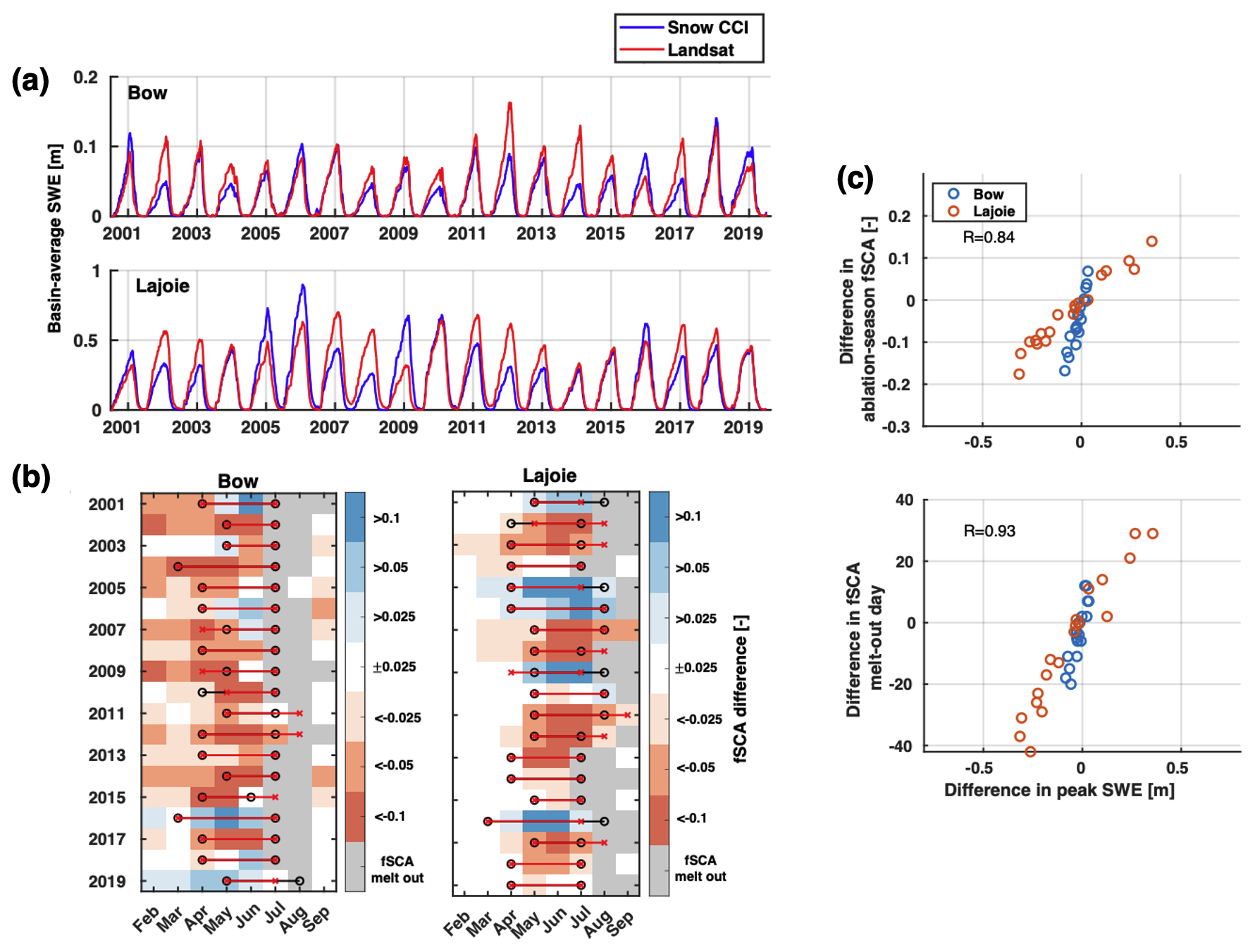
The comparison of the seasonal cycle of the basin-average SWE for the Bow and Lajoie domains is shown in Fig. 14a. The median seasonal cycle of Snow CCI posterior SWE generally matches the Landsat reanalysis with slightly negative differences. The full range of Snow CCI posterior SWE for the Lajoie domain is larger than that of Landsat posterior SWE, indicating a higher interannual variability. The spatial pattern of long-term peak SWE climatology from the Snow CCI reanalysis is compared with the Landsat reference (Fig. 14b and Table 6). Snow CCI and Landsat posterior peak SWE have similar spatial patterns with correlations of 0.82 and 0.8 for the Bow and Lajoie domains, respectively. Snow CCI and Landsat have comparable peak SWE for the Bow domain (mean difference of −0.04 m and RMSD of 0.09 m), whereas more significant differences exist in Lajoie with a mean difference of −0.13 m and RMSD of 0.34 m.

Figure 14 Same as Fig. 9 but for the Bow and Lajoie domains.

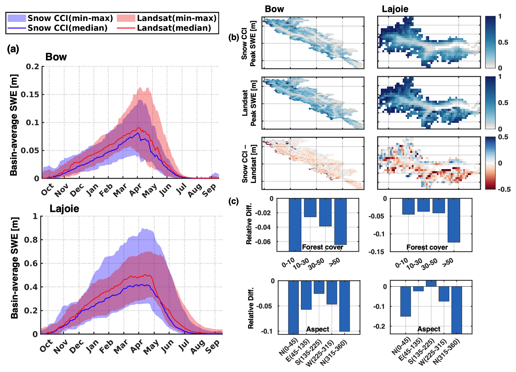
Table 6 Comparison statistics for the long-term median peak SWE between the Snow CCI and Landsat posterior estimates.

To investigate the impact of forest cover fraction and aspect on relative differences in peak SWE identified in the WUS example, we similarly bin the relative differences in long-term peak SWE from Snow CCI vs. Landsat according to forest cover and aspect (Fig. 14c). In both domains, relative differences generally become more negative as forest cover increases, with Bow forest cover of 0 %–10 % excepted. Note that the bar plots show mean relative differences in each bin as functions of forest cover and aspect. The poor performance in the Bow domain for forest cover of 0 %–10 % is likely due to outlier data points: when considering the median relative differences in each bin, the performance for 0 %–10 % forest cover is comparable to that of the 10 %–30 % range. Regions with south-facing slopes tend to exhibit less negative and positive relative differences in peak SWE. The largest (and most negative) relative differences in peak SWE are found on north-facing slopes for both domains, indicating that Snow CCI may underestimate fSCA over lower-illumination areas. Another hypothesis, as discussed in “Long-term SWE climatology” in Sect. 3.1.3, is that small snow-covered areas (low fSCA) may still exist on north-facing slopes during the warm season that are captured by the Landsat algorithm but are set to zero in Snow CCI by temperature threshold screening (Metsämäki et al., 2015). Additionally, forest-covered areas have a mixed-pixel temperature problem. SCAmod applies a snow temperature threshold to the combined components in a grid cell, but the temperatures of individual end-members (e.g., snow) provide more valuable information. Lundquist et al. (2018) developed a method to separate snow and forest temperatures using multispectral unmixing, leveraging differences in midwave and longwave infrared bands. Future work could explore whether this or a similar method can be applied across broader areas to address the mixed-pixel temperature issue affecting the Snow CCI fSCA product.

The interannual variability in basin-average SWE from the Snow CCI vs. Landsat reanalysis is displayed in Fig. 15a. The Snow CCI reanalysis generally yields comparable basin-average SWE relative to the Landsat results in most WYs. As was demonstrated in the WUS examples, significant fSCA differences in the ablation period lead to significant differences in basin-average peak SWE. This is also true in the Canadian test cases (Fig. 15c), as indicated by the correlation value of 0.84. It is also apparent that the earlier fSCA melt-out timing corresponds to the lower peak SWE and vice versa (Fig. 15c), and the correlation value is 0.93.

Figure 15 Same as Fig. 10 but for the Bow and Lajoie domains.

4 Conclusions

This study explored the potential for using the Snow CCI fSCA climate data record (CDR) to constrain mountain SWE estimates within a Bayesian SWE reanalysis framework. Four application domains spanning the WUS and western Canada with various physiographic and climatological conditions are used to evaluate its performance. Since Snow CCI fSCA is retrieved based on reflectance observations from the MODIS sensor, we applied the measurement error (standard deviation of 15 %) used for other MODIS-based product applications of the SWE reanalysis technique (Margulis et al., 2019). We acknowledge that a 15 % measurement error at nadir viewing is a simplification and that ideally the spatiotemporally varying estimate uncertainty built into the Snow CCI product would describe the uncertainty in the SCF estimates in a way that is meaningful for our data assimilation use case. We also consider the impact of viewing geometry and cloud cover but not canopy correction (Rittger et al., 2020).

Despite its relatively coarse spatial resolution (0.01°), assimilating Snow CCI fSCA typically resulted in improved posterior SWE estimates compared to the prior values in all four mountain test domains. In particular, assimilating Snow CCI fSCA improved both the temporal evolution (Figs. 7 and 13) and spatial pattern (correlation with ASO>0.75, Sect. 3.1.2) of the reanalysis SWE compared to in situ data (with some exceptions). A shortcoming of the SWE estimates resulting from assimilation of the Snow CCI product is that they are generally biased low at peak SWE based on comparisons with both in situ snow pillows (Tuolumne, Bow, and Lajoie) and ASO estimates (Tuolumne and Aspen).

Several additional conclusions stem from our comparisons of SWE estimates based on the Snow CCI product with those based on the Landsat product. First, we linked how differences in assimilated fSCA relate to differences in the posterior SWE values (Figs. 10 and 15). Positive (negative) relative biases in posterior SWE estimates from Snow CCI and Landsat are associated with higher (lower) fSCA values and a later (earlier) snow-free date. We hypothesize that these fSCA differences are due to differences in the products' respective retrieval algorithms and/or the spatial resolution of the raw reflectance measurements (Sect. 3.1.3). Secondly, these comparisons provided further evidence that Snow CCI posterior SWE is biased low overall. For all four domains, daily basin-wide climatological SWE estimates from the Snow CCI reanalysis are lower throughout the snow season compared to the Landsat reanalysis (Figs. 9a and 14a). In addition, the spatial pattern of long-term differences in peak SWE (Figs. 9c and 14c) demonstrates that these biases are affected by forest cover and aspect, where the magnitude of the Snow CCI reanalysis bias is largest in densely forested regions and north-facing aspects. Finally we also tied year-to-year differences in performance over the WUS to the number of high-quality fSCA scenes available during the ablation period (Fig. 11). This connection may also explain the poorer performance of the Landsat reanalysis over the two Canadian domains compared its performance over the WUS domains: the Canadian domains have limited good-quality fSCA scenes due to increased frequency of cloud cover and higher forest cover fraction.

The Snow CCI reanalysis presented herein aims to provide a methodology to fill the mountain SWE gap in the Snow CCI SWE CDR. The main challenges when extending this framework to untested regions and/or to other sensors (datasets) include (1) a bias correction of fSCA since the error covariance used in the reanalysis assumes unbiased measurements, (2) development of an algorithm to accurately identify cloud/warm surfaces from snow and setting an appropriate cloud fraction threshold for specific regions, and (3) accurate characterization of uncertainty in fSCA measurements. Another limitation to extending this work is the limited availability of spatially and/or temporally continuous reference data. Our temporal comparisons benefited from western North America's extensive snow pillow network, but spatial comparisons, which relied mainly on lidar-based SWE information, were limited outside of the WUS. Ongoing work includes characterizing the fSCA biases across different spatial and temporal (seasonal/annual) scales and correcting fSCA biases in canopy regions (Rittger et al., 2020). Additional tasks could include a detailed investigation of the benefits of using Snow CCI fSCA when Landsat measurements are limited (due to single Landsat tile coverage or significant cloud cover) or combining MODIS-derived Snow CCI estimates with higher-resolution estimates derived from Sentinel-2 measurements (Bair et al., 2023; Gascoin et al., 2020).