Importance of ice elasticity in simulating tide-induced grounding line variations along prograde bed slopes

The grounding line, delineating the boundary where a grounded glacier becomes afloat in ocean water, shifts in response to tidal cycles. Here, we analyze COSMO-SkyMed Differential Interferometric Synthetic Aperture Radar (DInSAR) data acquired in 2020 and 2021 over Totten, Moscow University, and Rennick glaciers in East Antarctica, detecting tide-induced grounding line position variations from 0.5 to 12.5 km along prograde slopes ranging from ∼ 0 % to 5 %. Considering a glacier as a non-Newtonian fluid, we provide two-dimensional formulations of viscous and viscoelastic short-term behavior of a glacier while in partial frictional contact with the bedrock and while partially floating on seawater. Since the models' equations are not amenable to analytical treatment, numerical solutions are obtained using FEniCS, an open-source Python package for solving partial differential equations using the finite element method. We establish the dependence of the grounding zone width on glacier thickness, bed slope, and glacier flow speed and find that grounding zone predictions using a viscoelastic model significantly outperform those of a purely viscous model. This study underscores the critical role played by ice elasticity in continuum-mechanics-based glacier models on daily timescales and demonstrates how these models can be validated using DInSAR measurements.

1 Introduction

The grounding line, which delineates the transition between the bedrock-based ice sheet and the floating ice shelf, is crucial for Antarctic research (Friedl et al., 2020; Haseloff and Sergienko, 2018). This boundary is a fundamental indicator of glacier stability, as its position reflects the glacier dynamics and influences the overall glacier force and mass balances (Davison et al., 2023; Holland, 2008). Grounding lines not only provide valuable information about glacier stability by enabling the evaluation of ice thickness, but also allow for the monitoring of sea level changes due to climate change (Goldstein et al., 1993; Schoof, 2007). Mechanisms governing variations in grounding line position are complex and involve both long-term and short-term processes (Sergienko and Haseloff, 2023; Sergienko, 2022). Short-term grounding line migrations are induced by tidal forces and occur within a tidal cycle (Albrecht et al., 2006; Coleman et al., 2002), while long-term migrations depend primarily on changes in ice dynamics and climate (Freer et al., 2023; Lowry et al., 2024). Models of grounding line evolution over timescales significantly exceeding tidal scales neglect short-term variations (Cornford et al., 2020; Gagliardini et al., 2016; Seroussi et al., 2014). Conversely, short-term glacier models focus on tidal timescales and tend to disregard the long-term evolution of glaciers due to its negligible impact over these shorter periods (Rosier et al., 2014; Rosier and Gudmundsson, 2020). Here, we focus on short-term, tide-induced grounding line migrations, which can extend up to several kilometers (Brancato et al., 2020; Brunt et al., 2010; Dawson and Bamber, 2017; Milillo et al., 2022; Minchew et al., 2017).

Several short-term glacier dynamics models, employing various physical approaches, have been developed to interpret tide-induced migrations. For example, a hydrological model proposed by Warburton et al. (2020) defines the grounding zone width as the penetration depth into a subglacial cavity of water interacting with an elastic ice beam that responds to ocean tides. Sayag and Worster (2011, 2013) describe grounding line migration as the result of tidal-force-induced deformation of an elastic Euler–Bernoulli beam which moves vertically in response to the periodic tidal forces. Tsai and Gudmundsson (2015) consider a grounding zone as an opening and closing of a crack between an elastic ice beam and the bedrock, using equations governing the propagation of a water-filled crack under pressure. This model (Tsai and Gudmundsson, 2015), which cannot predict grounding line migrations at low tides, was modified and applied to the Amery Ice Shelf in Antarctica by Chen et al. (2023), who showed that a crack model can reproduce a kilometer grounding line retreat over a tidal cycle. Nevertheless, the crack-based method is one-dimensional, as it considers only the glacier motion along the ice–bedrock surface without describing motion-induced changes within the ice.

Other previously proposed short-term models treat glacier ice as a viscous or viscoelastic fluid, aiming to determine grounding line migration by resolving contact forces at the base (Stubblefield et al., 2021). Rosier et al. (2014) and Rosier and Gudmundsson (2020) developed nonlinear viscoelastic models on tidal timescales, where normal stress and velocity determine the grounding line position. However, being considered after discretization, these factors are not incorporated into the variational formulation. This technical detail was addressed by Stubblefield et al. (2021), who used the Navier–Stokes equations for purely viscous flow and included contact conditions in the variational formulation. However, Stubblefield et al. (2021) did not compare the outputs of the viscous model with grounding zone width measurements. Here, we extend the viscous model proposed by Stubblefield et al. (2021) by incorporating an elastic component within the framework of the upper-convected Maxwell model (Gudmundsson, 2011; Snoeijer et al., 2020). The schematics of our study, presented in Fig. 1, show that glacier thickness, bedrock slope, and ice flow serve as model inputs and are set based on BedMachine Antarctica (Morlighem et al., 2017) and MEaSUREs InSAR-based ice velocity map of Antarctica (Rignot et al., 2017). We compare model results with grounding zone width measurements from Cosmo-SkyMed Differential Interferometric Synthetic Aperture Radar (DInSAR) data acquired between 2020 and 2021 over East Antarctica. Specifically, we focus on Totten (TOT), Moscow University (MU), and Rennick (REN) glaciers, which are characterized by kilometric tide-induced grounding line migrations. Comparing modeled and DInSAR-based grounding zones, we evaluate both models' performance and assess the significance of the elastic component relative to the formulation that accounts for only viscosity. Additionally, we assess the impact of the ice–bed system's main parameters, namely bedrock slope, glacier thickness, and ice velocity, on the magnitude of tidally induced grounding line migrations.

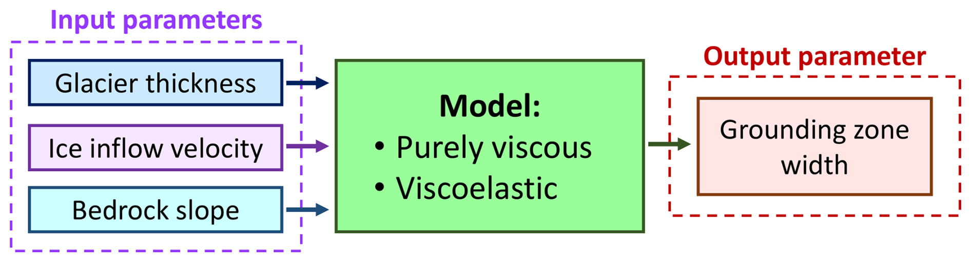
Figure 1 Schematic of the study. Grounding zone width is generated using either the viscous or viscoelastic model, with three input parameters: glacier thickness, ice inflow velocity, and bed slope.

2 Data and methods

2.1 Study area

This study focuses on three glaciers, MU, TOT, and REN, whose locations in Antarctica are shown in Fig. 2. MU and TOT are neighboring glaciers, located on the Sabrina Coast in East Antarctica (Bensi et al., 2022; Fernandez et al., 2018; Orsi and Webb, 2022). Together, the combined effect of these two glaciers may result in up to a 5 m sea level rise, making them major contributors to sea level changes in East Antarctica (Mohajerani et al., 2018). Being characterized by the highest outflow and thinning rate in East Antarctica, TOT also has the third-largest ice flux among all Antarctic glaciers, following Pine Island and Thwaites glaciers (Pritchard et al., 2009; Rignot and Thomas, 2002; Roberts et al., 2018). In contrast, MU exhibits relatively slow thinning rates compared to TOT (Mohajerani et al., 2018). For instance, between 2010 and 2019, the surface thinning rate of MU was nearly half of that for TOT: 0.9 m yr⁻¹ vs. 1.64 m yr⁻¹ (Li et al., 2022). Moreover, between 2010 and 2018, both glaciers experienced higher basal melt rates than the neighboring glaciers in East Antarctica due to the intrusion of warm ocean water into their subglacial cavities (Adusumilli et al., 2020; Li et al., 2022; Nitsche et al., 2017).

REN, situated in northern Victoria Land in East Antarctica, spans over 400 km along the flow and narrows from 80 to 25 km across the flow (Allen et al., 1985; Mayewski et al., 1979; Meneghel et al., 1999; Sturm and Carryer, 1970). Containing the sea level equivalent of 11 cm in the form of ice, REN is also grounded below the sea level and is experiencing rapid thinning due to intensive basal melt (Adusumilli et al., 2020; Rignot et al., 2019). REN's ice discharge has shown up to 20 % amplification between 1999 and 2018 (Miles et al., 2022). Although REN behaves similarly to TOT and MU, it retreats slower than most Antarctic glaciers, rendering it relatively stable (Baumhoer et al., 2021; Miles et al., 2022).

2.2 Glacier parameters used as model inputs

Since the model requires glacier thickness, bed slopes, and ice speed as input parameters, we estimated these values for the three glaciers of interest. To achieve this, we determined 69 profile lines: 33 lines over MU, 17 over TOT, and 19 over REN (Fig. 2).

2.2.1 SAR-based ice flow velocities

The profiles were oriented in the direction of ice flow, derived from the synthetic aperture radar (SAR)-based ice velocity map of Antarctica (Rignot et al., 2017), provided by NASA's MEaSUREs program. This dataset includes the v_x and v_y components of the ice velocities v in meters per year (m yr⁻¹), projected to EPSG3031 at 450 m resolution. The direction of the ice flow was calculated in degrees and is shown with black arrows in Fig. 2. For the direction calculation, we utilized Python's $\mathrm{np}.\arctan \mathrm{2}\left(v_y,v_x\right)$ function to ensure full 360° coverage (https://numpy.org/doc/2.1/reference/generated/numpy.arctan2.html, last access: 20 May 2024). Flow lines were selected along the direction of the ice flow and were spaced 500 to 600 m apart. However, due to the 400 m grounding zone mapping error, we did not position the profiles in areas where the grounding zone width is less than 400 m, which resulted in a larger spacing between MU's profiles 25 and 26. Each profile, centered on the grounding zone, is approximately 20 km long, as this length was adopted as the glacier domain length for the modeling process. The flow lines, and consequently the selected profiles, are not always perpendicular to the grounding lines, indicating the influence of crossflow heterogeneity in our analysis. To estimate the flow speed, we calculated the magnitude of the ice flow vectors (or the velocity map) as $\sqrt{v_x^{\mathrm{2}}+v_y^{\mathrm{2}}}$, extracted the values from the velocity map along the profile lines, and computed the average ice flow for each profile. The summary of the calculated ice flow velocities along the selected 69 profiles is provided in Table S1 in the Supplement.

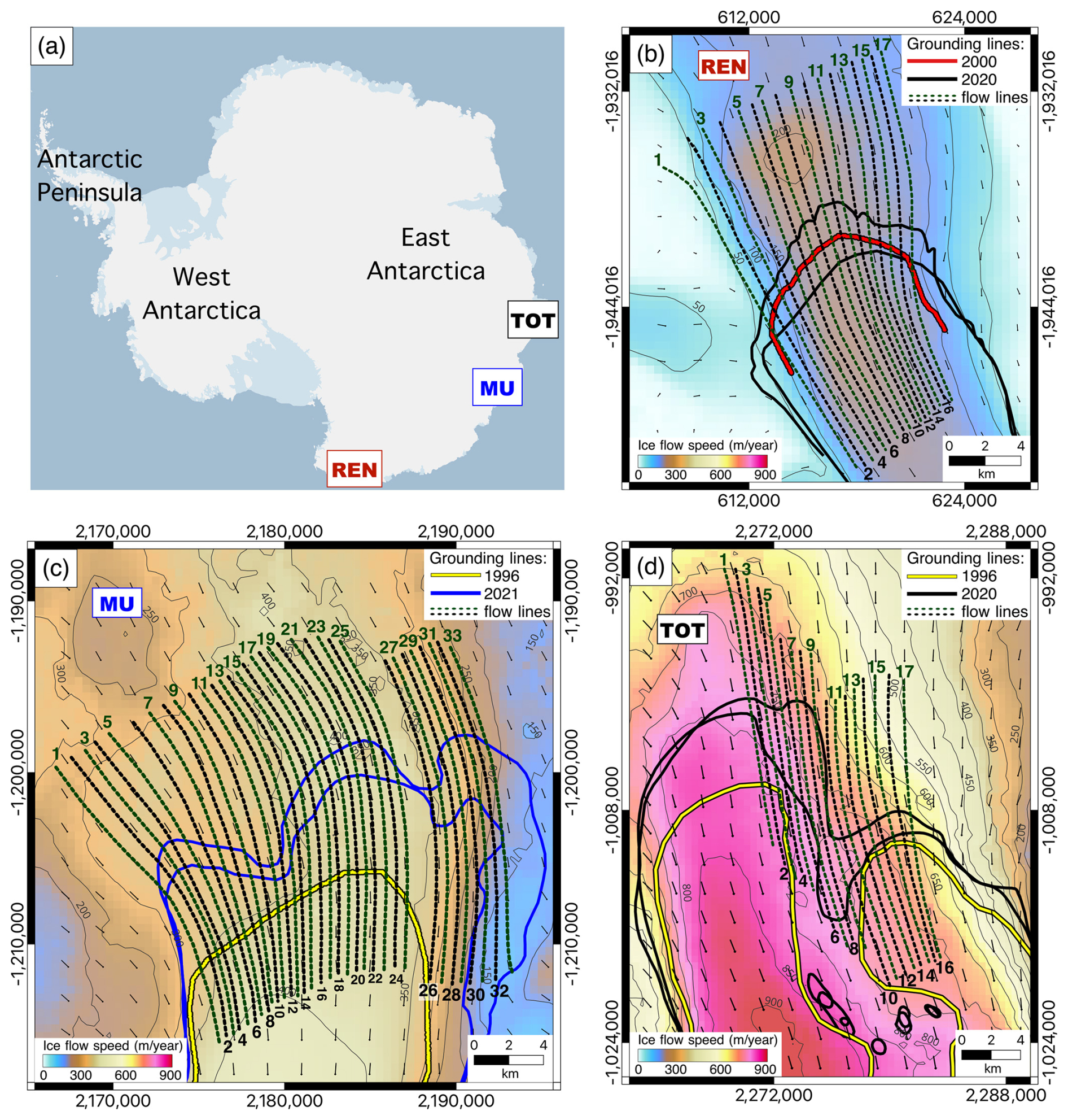
Figure 2 Study area: (a) location of TOT, MU, and REN in Antarctica and ice velocity map over (b) REN, (c) MU, and (d) TOT. The selected 69 profiles are shown as dashed green and black lines over the black ice flow vectors, derived from the MEaSUREs InSAR-based ice velocity map of Antarctica (Rignot et al., 2017). For visualization purposes, the flow vectors shown here were calculated over a velocity flow map resampled at 2 km, while the directions of the profiles were determined over the original 450 m resolution flow map to maximize the accuracy of the flow direction definition. The grounding lines over REN and TOT were mapped in 2020 (black line), while the grounding lines over MU (blue line) correspond to 2021. The grounding lines for 1996 (yellow line) and 2000 (red line) were taken from the MEaSUREs DInSAR-based Antarctic grounding line dataset (Rignot et al., 2016). All maps are represented in Antarctic projection (EPSG:3031).

2.2.2 Ice thickness and bed slope

Glacier thickness values were determined using the 500 m resolution ice thickness map from BedMachine Antarctica (version 2) (Morlighem et al., 2017), as shown in Fig. 3. Thickness values were extracted along the profiles, and the average thickness was calculated for each profile. Bed slopes for each profile were determined using the 500 m resolution BedMachine Antarctica topographic map (Fig. 3) by linearly approximating extracted bed elevation values and calculating the slope of the fitted line. The summary of the calculated glacier thicknesses and bed slopes along the selected 69 profiles is provided in Table S1.

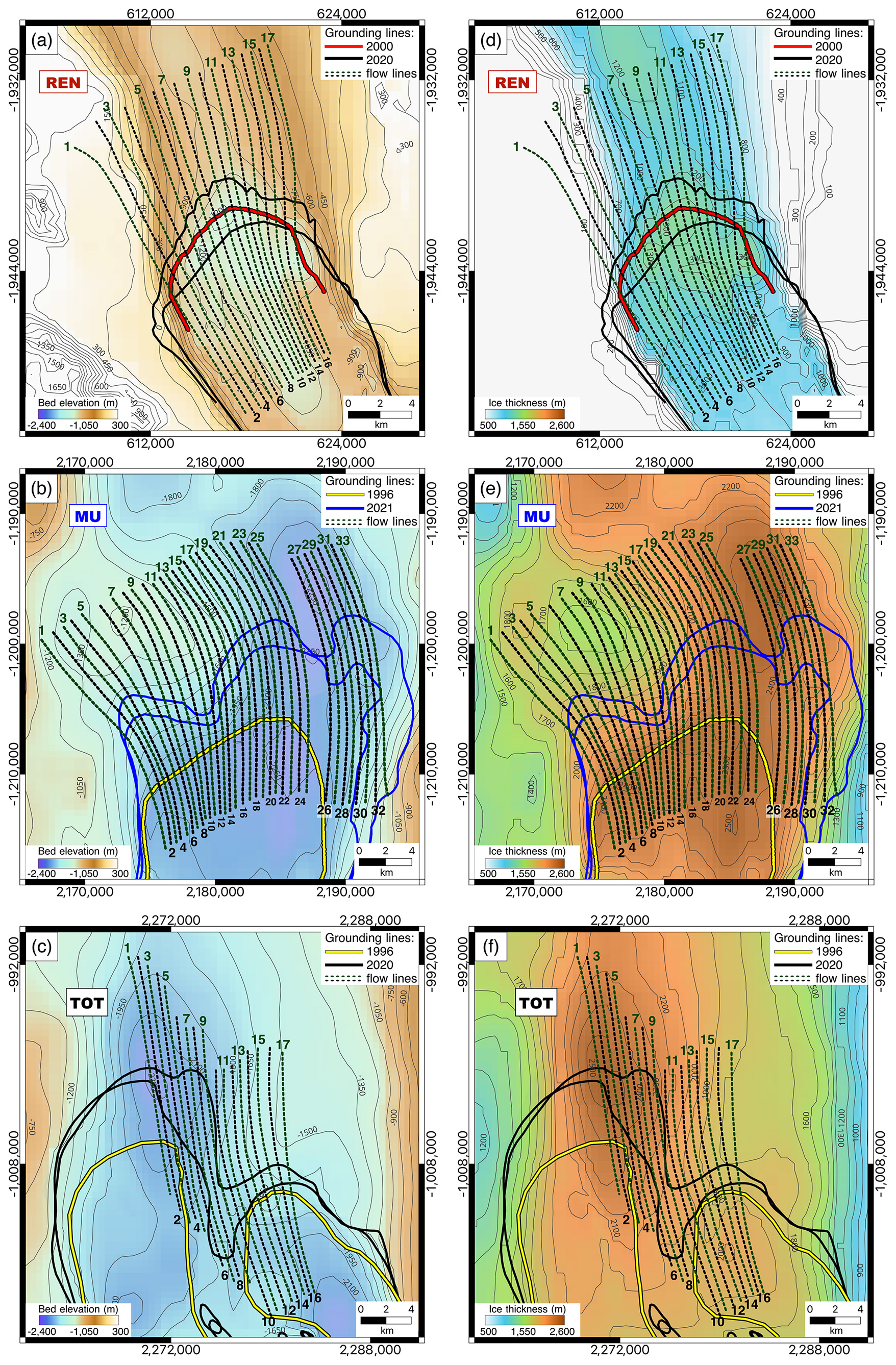
Figure 3 Bed elevation from BedMachine2 (Morlighem et al., 2017) over (a) REN, (b) MU, and (c) TOT and ice thickness maps from BedMachine2 (Morlighem et al., 2017) over (d) REN, (e) MU, and (f) TOT. The selected 69 profiles are shown as dashed green and black lines. The grounding lines over REN and TOT were mapped in 2020 (black line), while the grounding lines over MU (blue line) correspond to 2021. The grounding lines for 1996 (yellow line) and 2000 (red line) were taken from the MEaSUREs DInSAR-based Antarctic grounding line dataset (Rignot et al., 2016). All maps are represented in Antarctic projection (EPSG:3031).

2.3 DInSAR-based grounding zone widths for model validation

As the model estimates grounding zone values, grounding zone measurements are required to assess the model performance. We obtained the grounding zone width values for TOT, MU, and REN by utilizing a series of 1 d repeat-pass synthetic aperture radar (SAR) data from the COSMO-SkyMed (CSK) mission, operated by the Italian Space Agency (ASI). The first generation of the mission comprises a constellation of four satellites equipped with synthetic aperture radars operating at X-band with a wavelength of 3.1 cm (Milillo et al., 2014). Each of the four first-generation satellites has a 16 d repeat cycle, while the second and third satellites capture InSAR data over the same area with a 1 d interval. Interferograms were generated using GAMMA software (Werner et al., 2000) from CSK STRIPMAP data, following a validated processing chain (Brancato et al., 2020; Milillo et al., 2017). Satellite acquisitions were designed as a set of five consecutive overlaying 40 km ×40 km swath frames with an azimuth and range resolution of 3 m. To eliminate topographic effects, the Copernicus digital elevation model (DEM) is employed. To co-register the data and achieve maximum phase coherence, we used satellite orbits for coarse co-registration and used a pixel offset approach for fine co-registration. A multi-looking factor of 10 in both range and azimuth was used to achieve an interferogram resolution of 30 m × 30 m. Two 1 d interferometric pairs were combined into one double-differential interferogram (DInSAR) to cancel out horizontal deformation due to glacier flow. Each interferometric pair combined in a double-difference DInSAR interferogram is acquired within 1.5 months over the same satellite track to minimize horizontal velocity changes and highlight vertical glacier motion, enabling grounding line mapping (Milillo et al., 2022). Double-difference DInSAR interferograms from different orbits acquired at different times ensured sensitivity to several frequencies of the tidal spectrum (Milillo et al., 2017; Minchew et al., 2017).

An interferometric fringe corresponds to half a wavelength of surface displacement, equivalent to 1.5 cm of satellite line-of-sight displacement per fringe for X-band or about 1.7 cm when projecting deformation onto the vertical considering the satellite incidence angle. The grounding line can be manually delineated as the most inner fringe in the grounded ice side. Therefore, the DInSAR technique provides information about vertical tide-induced glacier movements and enables manual grounding line mapping with an average empirically determined manual mapping accuracy of 100–200 m (Rignot et al., 2014; Ross et al., 2024a). To connect the models with the observations, we needed to link every SAR image to its unique sea level and atmospheric pressure level, which also introduced vertical displacement due to the inverse barometer effect (IBE) (Padman et al., 2002). The IBE correction was performed by examining anomalies in mean sea level pressure, reconstructed using the fifth generation of the European Centre for Medium-Range Weather Forecasts (ECMWF) atmospheric reanalysis dataset of the global climate (ERA-5; Table S2) (Hersbach et al., 2020). The tidal heights during the acquisition of the SAR images were determined using the Circum-Antarctic Tidal Simulation (CATS2008) model (Padman et al., 2002) and are listed in Table S2. Despite one double-difference DInSAR interferogram being a combination of four SAR images, characterized by four different sea levels, one DInSAR interferogram provided only one grounding line measurement. A high tide lifts the glacier, allowing seawater to penetrate under the glacier, while a low tide causes the glacier to readvance. Following Milillo et al. (2022), we assumed that the grounding line position observed in a DInSAR interferogram corresponds to the largest combination of tidal level and IBE among the four SAR acquisitions. Following this assumption our approach will never be able to map the grounding line at its lowest tidal position. To estimate the grounding zone width for one glacier, we used a pair of double-difference DInSAR interferograms. A maximum acquisition gap of 1.5 months between the interferograms in a pair ensures that any variations in the grounding line position occur due to the tidal interaction rather than glacier retreat (Milillo et al., 2022). The difference between the largest IBE-corrected tidal heights (column H in Table S2) in each pair of DInSAR interferograms is 0.95 m for MU, 1.03 m for TOT, and 1.08 m for REN (column H in Table S2). For each pair of interferograms, the interferogram with the higher H value represents the inland position of the grounding line and corresponds to the ocean tide, referred to as “high tide” in the model. Conversely, the interferogram with the lower H value represents the outward position of the grounding line, corresponding to “low tide” in the model. To ensure a valid comparison between the DInSAR-derived grounding zones and the modeled grounding zones, the IBE-corrected tidal levels listed in column H of Table S2 are used to evaluate the grounding zone width in the model. We measure the modeled grounding zone widths by calculating the difference between the grounding line position at maximum H and at minimum H.

Combining two manually mapped grounding lines for each interferogram in a pair, we established a grounding zone for the corresponding glacier and measured the grounding zone widths along the selected profiles. Therefore, one pair of DInSAR interferograms for MU allowed us to obtain 33 grounding zone width values, as 33 profiles were originally selected over this glacier. Analogously, we obtained 19 grounding zone widths for REN and 17 for TOT. Taking the higher limit of the grounding line mapping error of 200 m (Rignot et al., 2014; Ross et al., 2024a), we determined the largest level of uncertainty of 400 m for each grounding zone measurement due to error propagation (see measurement error bars in Fig. 7c). The summary of the grounding zone width measurements is provided in Table S1, and the grounding zone width measurement process for MU, TOT, and REN is visualized in Fig. 4, which shows all three pairs of DInSAR interferograms, corresponding to low and high tide, and the 69 profiles along which the grounding zone width measurements were performed.

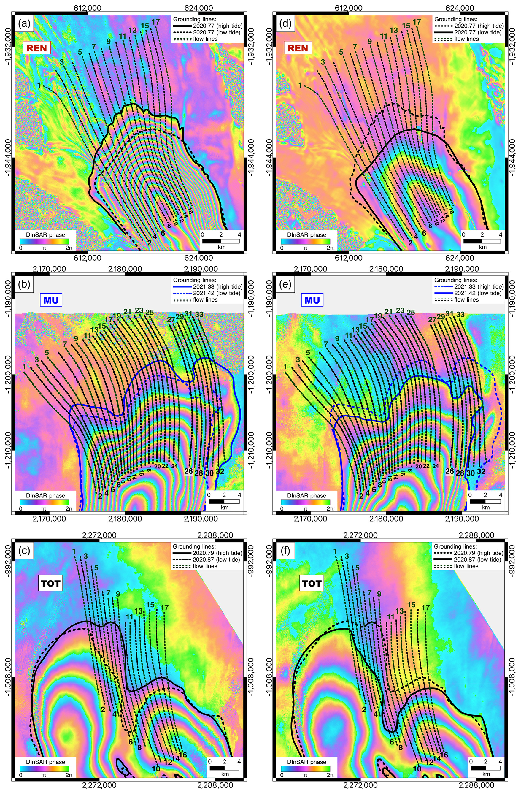
Figure 4 Pairs of DInSAR interferograms over (a) REN, (b) MU, and (c) TOT at high tide and over (d) REN, (e) MU, and (f) TOT at low tide with corresponding manually mapped grounding lines. All interferograms are represented in Antarctic projection (EPSG:3031).

3 Viscous and viscoelastic models

The short-term grounding line migration model, rooted in the Navier–Stokes equations under the assumption of viscoelastic ice flow, builds upon the purely viscous formulation of the same problem (Stubblefield et al., 2021). Here, we provide the comprehensive description of the viscoelastic model along with a comparison between the viscous and viscoelastic models. The notation used in the paper is listed in Table S3 and is further explained during the model formulation. In addition to summarizing the quantities and their corresponding mathematical symbols, Table S3 also provides the units and identifies the field type to which each quantity belongs, such as scalar, vector, or tensor field.

3.1 Glacier domain

For both models, we designate the glacier domain as Ω, as shown in Fig. 5, with a piecewise smooth boundary ∂Ω. We place the glacier in a two-dimensional coordinate system (XY), where X denotes the horizontal axis, and Y is used for identifying the vertical axis. In the principal notation used in this paper, a spatial point is denoted by $x=\left(xy\right)\in \stackrel{\mathrm{‾}}{\mathrm{\Omega }}$, where an overline denotes the set closure. For glacier length L, the ice domain Ω can be mathematically expressed as

$$\begin{array}{}\text{(1)}& \mathrm{\Omega }=\left\{\left(x,y\right):\left|x\right|<{\displaystyle \frac{L}{\mathrm{2}}},s\left(x,t\right)<y<h\left(x,t\right)\right\}.\end{array}$$

The glacier boundary is represented as a union of five complementary parts:

$$\begin{array}{}\text{(2)}& \partial \mathrm{\Omega }={\mathrm{\Gamma }}_D\cup {\mathrm{\Gamma }}_N\cup {\mathrm{\Gamma }}_{\mathrm{w}}\cup {\mathrm{\Gamma }}_{\mathrm{b}}\cup {\mathrm{\Gamma }}_a,\end{array}$$

where Γ_D is an inflow boundary, Γ_N is an outflow boundary, Γ_w is an ice–water surface, Γ_b is an ice–bedrock surface, and Γ_a is an ice–air surface. Defining b(x) as a bedrock slope function, h(xt) as a time-dependent function of the glacier surface elevation, and s(xt) as a function, defining the position of lower boundary of the ice shelf with time, the ice–water and ice–bed boundaries are expressed as

$$\begin{array}{}\text{(3)}& {\displaystyle }{\mathrm{\Gamma }}_{\mathrm{w}}=\left\{\left(x,y\right)\in \partial \mathrm{\Omega }:y=s\left(x,t\right)>b\left(x\right)\right\},\text{(4)}& {\displaystyle }{\mathrm{\Gamma }}_{\mathrm{b}}=\left\{\left(x,y\right)\in \partial \mathrm{\Omega }:y=s\left(x,t\right)=b\left(x\right)\right\}.\end{array}$$

The entire lower boundary Γ_s, therefore, is identified as a union of the ice–water and ice–bed boundaries:

$$\begin{array}{}\text{(5)}& {\mathrm{\Gamma }}_{\mathrm{s}}={\mathrm{\Gamma }}_{\mathrm{w}}\cup {\mathrm{\Gamma }}_{\mathrm{b}}=\left\{\left(x,y\right)\in \partial \mathrm{\Omega }:y=s\left(x,t\right)\ge b\left(x\right)\right\}.\end{array}$$

The grounding line position is the point where the ice–water boundary intersects the ice–bed boundary.

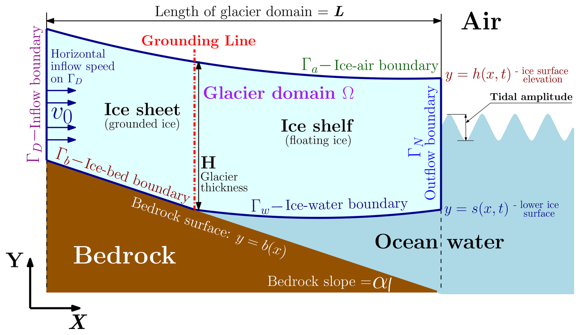
Figure 5 Model geometry for both viscous and viscoelastic problems, highlighting the ice domain Ω boundaries, as defined in Table S3.

3.2 Model formulation

Here, we describe the formulation of both models, which have the same domain and boundary conditions but different governing equations. The summary of the notation mentioned here is provided in Table S3.

3.2.1 Governing equations

In both models, a glacier behaves as an incompressible non-Newtonian fluid, either viscous or viscoelastic. Incompressibility means that the fluid density does not change during flow, which mathematically implies zero divergence of the flow velocity v:

$$\begin{array}{}\text{(6)}& \mathrm{\nabla }\cdot v=\mathrm{0}.\end{array}$$

Both models are described by Cauchy's first law of motion under quasi-static conditions, which provides the momentum conservation, expressed as

$$\begin{array}{}\text{(7)}& \mathrm{\nabla }\cdot T\left(v,p\right)+{\mathit{\rho }}_{i}g=\mathrm{0},\end{array}$$

where T is the Cauchy stress tensor, ρ_i is the ice density, and g is the gravitational acceleration vector which in the glacier reference system is identified as $g=g(\mathrm{0}-\mathrm{1}{)}^T$ with magnitude g.

The difference between the models becomes apparent when considering the constitutive law, which defines the physical nature of the models. The viscous model is described by the following equation:

$$\begin{array}{}\text{(8)}& T\left(v,p\right)=-pI+\mathrm{2}\mathit{\eta }\left(D\right)D,\end{array}$$

where p is the ice pressure, I is a second-order identity tensor, η(D) is a velocity-dependent ice viscosity, and D is a strain rate tensor.

$$\begin{array}{}\text{(9)}& D\left(v\right)={\displaystyle \frac{\mathrm{1}}{\mathrm{2}}}\left[\mathrm{\nabla }v+(\mathrm{\nabla }v{)}^T\right]\end{array}$$

Ice viscosity in the viscous model is identified via Glen's flow as

$$\begin{array}{}\text{(10)}& \mathit{\eta }\left(D\right)={\mathrm{2}}^{\frac{-\mathrm{1}-n}{\mathrm{2}n}}\cdot \sqrt[-n]{A}{\left({\left|D\left(v\right)\right|}^{\mathrm{2}}+\mathit{\delta }\right)}^{\frac{\mathrm{1}-n}{\mathrm{2}n}},\end{array}$$

where n≥1 is the stress exponent, A>0 is the ice softness, and δ≪1 is an infinitesimal numerical parameter used to prevent numerical instability of the models at zero strain rate.

For the viscoelastic model, constitutive law (8) and the viscosity expression (10) are principally different. We consider the Maxwell model of viscoelasticity, which considers both viscous and elastic components. The Maxwell model assumes that deformation properties can be represented by a purely elastic spring and a purely viscous dashpot connected in series. Therefore, in the Maxwell model, a viscoelastic material behaves as a purely viscous flow under slow deformation (long timescale), while it exhibits elastic resistance to rapid deformations (short timescale). However, since the simple Maxwell model describes small deformations, we apply the upper-convected Maxwell model, which includes some geometrical nonlinearity. The constitutive relation for the viscoelastic model is identified as

$$\begin{array}{}\text{(11)}& T\left(v,p\right)=-pI+\mathit{\tau },\end{array}$$

where, compared to the purely viscous model (8), the strain rate tensor D (Eq. 9) is replaced with the deviatoric stress tensor τ, which is strain-rate-dependent:

$$\begin{array}{}\text{(12)}& \mathit{\tau }+\mathit{\lambda }\mathrm{\nabla }\mathit{\tau }-\mathrm{2}\mathit{\eta }\left(\mathit{\tau }\right)D\left(v\right)=\mathrm{0},\end{array}$$

where $\mathit{\lambda }=\frac{\mathit{\eta }\left(\mathit{\tau }\right)}{G}$ is the relaxation time with the shear modulus G, and ∇τ is the upper-convected time derivative of τ. The viscoelastic model reduces to the viscous model described in Stubblefield et al. (2021) when λ=0, while at infinitely big λ, the upper-convected Maxwell model reduces to a neo-Hookean elastic solid (Snoeijer et al., 2020). The ice viscosity in Eq. (12) is

$$\begin{array}{}\text{(13)}& \mathit{\eta }\left(\mathit{\tau }\right)={\displaystyle \frac{\mathrm{1}}{\mathrm{2}A|\mathit{\tau }{|}^{n-\mathrm{1}}}}.\end{array}$$

The upper-convected time derivative ∇τ can be found as

$$\begin{array}{}\text{(14)}& \mathrm{\nabla }\mathit{\tau }={\displaystyle \frac{D\mathit{\tau }}{Dt}}-{\left(\mathrm{\nabla }v\right)}^T\cdot \mathit{\tau }-\mathit{\tau }\cdot \mathrm{\nabla }v,\end{array}$$

where $\frac{D\mathit{\tau }}{Dt}=\frac{\partial \mathit{\tau }}{\partial t}+v\cdot \mathrm{\nabla }\mathit{\tau }$ is the material derivative of τ. The partial time derivative of τ on the current time step is calculated using the value from the previous time step, applying the backward Euler approximation:

$$\begin{array}{}\text{(15)}& {\displaystyle \frac{\partial \mathit{\tau }(x,t)}{\partial t}}={\displaystyle \frac{\mathit{\tau }\left(x,t\right)-\mathit{\tau }(x,t-\mathrm{\Delta }t)}{\mathrm{\Delta }t}}.\end{array}$$

3.2.2 Evolution of the lower boundary

The time evolution of the lower boundary $y=s(x,t)$ is governed by the kinematic equation, which states that the surface moves with the ice flow. Assuming no mass changes at the lower surface, such as melting or freezing, the equation can be written as (Hirt and Nichols, 1981; Schoof, 2011)

$$\begin{array}{}\text{(16)}& {\displaystyle \frac{\partial s}{\partial t}}+v_x{\displaystyle \frac{\partial s}{\partial t}}=v_y,\end{array}$$

where v_x and v_y are the components of the surface velocity vector $v{\mathrm{|}}_{\mathrm{s}}={\left(v_x,v_y\right)}^T$. Rewriting Eq. (16) in terms of the outward-pointing normal to the lower boundary $\widehat{n}{\mathrm{|}}_{\mathrm{s}}=\frac{{\left(\frac{\partial s}{\partial x},-\mathrm{1}\right)}^T}{\sqrt{\mathrm{1}+{\left(\frac{\partial s}{\partial x}\right)}^{\mathrm{2}}}}$, we get

$$\begin{array}{}\text{(17)}& {\displaystyle \frac{\partial s}{\partial t}}=-v\cdot \widehat{n}{\mathrm{|}}_{\mathrm{s}}\cdot \sqrt{\mathrm{1}+{\left({\displaystyle \frac{\partial s}{\partial x}}\right)}^{\mathrm{2}}}.\end{array}$$

Since the solution of Eq. (17) is numerically unstable (Durand et al., 2009), we apply the backward Euler method to remove the instability. Denoting the approximate solution on kth time step as s_∗, such as $s_{\ast }\equiv s\left(x,t_k\right)$, and applying the backward Euler method to equation (17) under the assumption that ${\left(\frac{\partial s}{\partial x}\right)}^{\mathrm{2}}\ll \mathrm{1}$, we get

$$\begin{array}{}\text{(18)}& s_{\ast }\left(x,t_k\right)=s\left(x,t_k-\mathrm{\Delta }t\right)-\mathrm{\Delta }t\cdot v_{\mathrm{n}}\left(x,s,t_k\right),\end{array}$$

where $v\cdot \widehat{n}{\mathrm{|}}_{\mathrm{s}}$ was replaced with v_n. We assume that the ocean is hydrostatic and define p_w as the water pressure at the ice–water interface and $p_{\mathrm{w}}^{\mathrm{0}}$ as the hydrostatic water pressure. If l is sea level, the hydrostatic water pressure at kth time step is governed by the following equation:

$$\begin{array}{}\text{(19)}& p_{\mathrm{w}}^{\mathrm{0}}\left(xs{t}_k\right)={\mathit{\rho }}_{\mathrm{w}}g\left(l\left(t_k\right)-s_{\ast }(x,t_k)\right).\end{array}$$

3.2.3 Boundary conditions

Identifying $\widehat{n}\left(\mathbf{x}\right)$ as a unit outward normal vector at some point x of any domain boundary, we determine an orthogonal projection onto that boundary as a second-order tensor P:

$$\begin{array}{}\text{(20)}& \mathbb{P}:=\mathbb{I}-\widehat{n}\left(x\right)\otimes \widehat{n}\left(x\right),\end{array}$$

where ⊗ is the tensor product. Denoting ⋅ as an inner product, we also define the projection of the Cauchy stress tensor T as

$$\begin{array}{}\text{(21)}& T_{\mathrm{n}}=-\widehat{n}\cdot T\cdot \widehat{n}.\end{array}$$

Both models use the same Dirichlet boundary conditions provided in Table 1, where v₀>0 is the horizontal ice flow speed on the inflow boundary Γ_D.

Table 1 Models' boundary conditions.

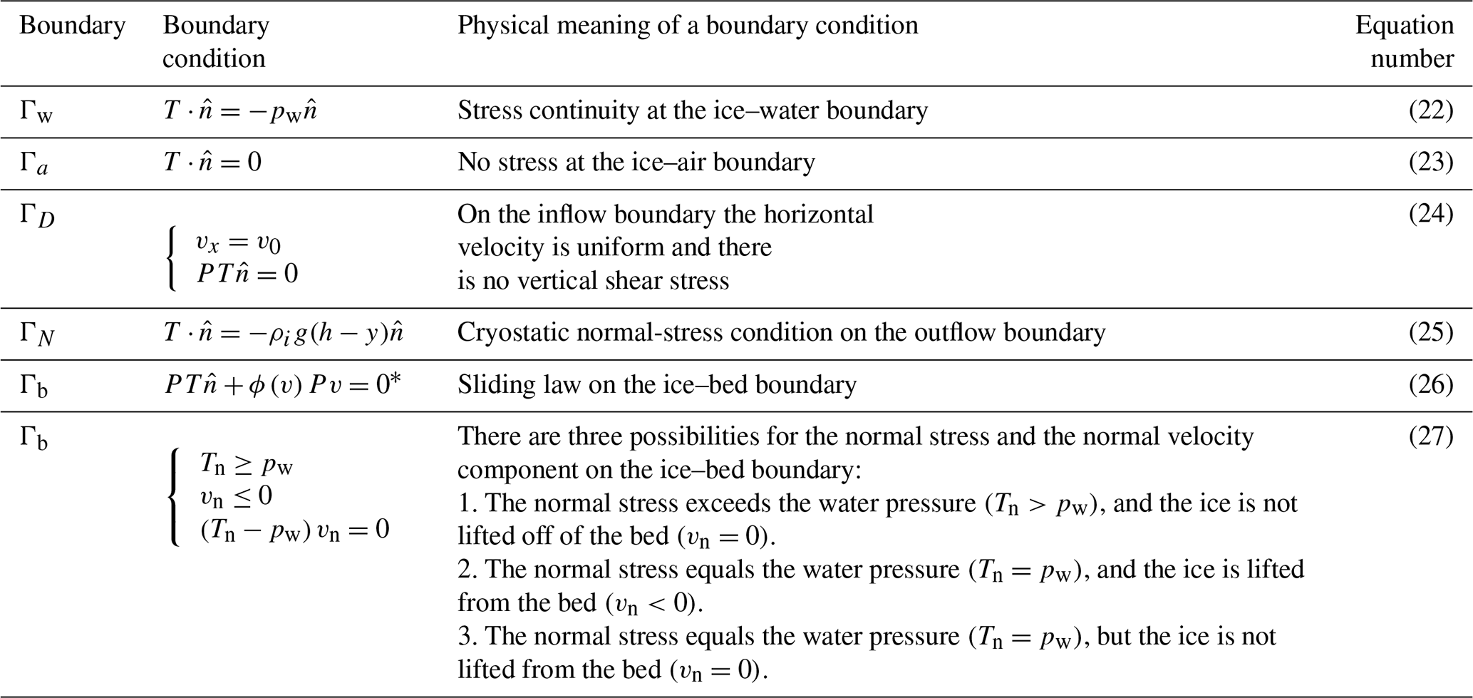
^* In Eq. (26), $\mathit{\varphi }\left(v\right)=C{\left(\mathrm{|}Pv{\mathrm{|}}^{\mathrm{2}}+\mathit{\epsilon }\right)}^{\frac{\mathrm{1}-n}{\mathrm{2}n}}$ is friction with friction coefficient C and numerical parameter ε≪1 (in m² s⁻²) used to prevent numerical instabilities.

3.3 Viscoelastic model weak formulation

In this subsection, we provide the derivation of the viscoelastic model, while the viscous model is derived in Stubblefield et al. (2021). Let us define V as the velocity function space. K is a closed, convex subset of V such that

$$\begin{array}{}\text{(28)}& K=\left\{v\in V:v_{\mathrm{n}}{\mathrm{|}}_{{\mathrm{\Gamma }}_{\mathrm{b}}}\le \mathrm{0}\text{and}{v}_x{\mathrm{|}}_{{\mathrm{\Gamma }}_D}=v_{\mathrm{0}}\right\}.\end{array}$$

Multiplying Eq. (7) by v−u (where u∈K is an arbitrary test function) and integrating the expression over the glacier domain Ω, in the indicial notation we will get

$$\begin{array}{}\text{(29)}& \underset{\mathrm{\Omega }}{\int }(v_k-u_k)T_{kj,j}\mathrm{d}V+\underset{\mathrm{\Omega }}{\int }{\mathit{\rho }}_i{g}_k(v_k-u_k)\mathrm{d}V=\mathrm{0}.\end{array}$$

Integrating the first integral in Eq. (29) by parts and applying the divergence theorem (Green's identity), we then apply Eq. (11) to one of the integrals and rewrite the resulting expression in tensor notation:

$$\begin{array}{}\text{(30)}& \begin{array}{rl}& -\underset{\partial \mathrm{\Omega }}{\int }T\cdot \widehat{n}\cdot (v-u)\mathrm{d}a+\underset{\mathrm{\Omega }}{\int }\mathit{\{}-p\mathrm{\nabla }\cdot \left(v-u\right)\\ & +\mathit{\tau }\cdot \mathrm{\nabla }(v-u)-{\mathit{\rho }}_{i}g(v-u)\mathit{\}}\mathrm{d}V=\mathrm{0}.\end{array}\end{array}$$

Now, we decompose ∂Ω onto the compounding boundaries (see Eq. 2) and consider the first integral in Eq. (30) over each boundary separately. Using Eqs. (20) and (21) and boundary condition in Eq. (26) on Γ_b, after integration over Γ_b and taking into account that T_n≥p_w on Γ_b, we derive the following:

$$\begin{array}{}\text{(31)}& \begin{array}{rl}& -\underset{{\mathrm{\Gamma }}_{\mathrm{b}}}{\int }T\cdot \widehat{n}\cdot (v-u)\mathrm{d}a\le \underset{{\mathrm{\Gamma }}_{\mathrm{b}}}{\int }\mathit{\alpha }\left(v\right)\cdot \mathbb{P}v\cdot \mathbb{P}(v-u)\mathrm{d}a\\ & +\underset{{\mathrm{\Gamma }}_{\mathrm{b}}}{\int }{p}_{\mathrm{w}}(v_{\mathrm{n}}-u_{\mathrm{n}})\mathrm{d}a.\end{array}\end{array}$$

On Γ_w, from Eq. (22), we obtain the following expression:

$$\begin{array}{}\text{(32)}& -\underset{{\mathrm{\Gamma }}_{\mathrm{w}}}{\int }T\cdot \widehat{n}\cdot \left(v-u\right)\mathrm{d}a=\underset{{\mathrm{\Gamma }}_{\mathrm{w}}}{\int }{p}_{\mathrm{w}}\left(v_{\mathrm{n}}-u_{\mathrm{n}}\right)\mathrm{d}a.\end{array}$$

On Γ_D, from Eq. (24), we have $\mathbb{P}T\widehat{n}=\mathrm{0}$; thus, this boundary does not contribute to the integral $\underset{\partial \mathrm{\Omega }}{\int }T\cdot \widehat{n}\cdot (v-u)\mathrm{d}a$. On Γ_a, from Eq. (23), we have $T\cdot \widehat{n}=\mathrm{0}$; thus, this ice–air boundary does not contribute to the integral $\underset{\partial \mathrm{\Omega }}{\int }T\cdot \widehat{n}\cdot (v-u)\mathrm{d}a$ as well. On Γ_N, from Eq. (25), we know $T\cdot \widehat{n}=-{\mathit{\rho }}_{i}g(h-y)\widehat{n}$, which means that the contribution from the boundary to $\underset{\partial \mathrm{\Omega }}{\int }T\cdot \widehat{n}\cdot (v-u)\mathrm{d}a$ will be

$$\begin{array}{}\text{(33)}& -\underset{{\mathrm{\Gamma }}_N}{\int }T\cdot \widehat{n}\cdot (v-u)\mathrm{d}a=\underset{{\mathrm{\Gamma }}_N}{\int }{\mathit{\rho }}_{i}g\left(h-y\right)(v_{\mathrm{n}}-u_{\mathrm{n}})\mathrm{d}a.\end{array}$$

Substituting Eqs. (31)–(33) with Eq. (30), replacing the union of Γ_w and Γ_b with Γ_s, and replacing p_w with $p_{\mathrm{w}}={\mathit{\rho }}_{\mathrm{w}}g(l-s+\mathrm{\Delta }t\cdot v_{\mathrm{n}})$, which was derived from Eqs. (18) and (19), we obtain

$$\begin{array}{}\text{(34)}& \begin{array}{rl}\underset{\mathrm{\Omega }}{\int }\mathit{\{}-p\mathrm{\nabla }\cdot \left(v-u\right)& +\mathit{\tau }\cdot \mathrm{\nabla }\left(v-u\right)-{\mathit{\rho }}_{i}g\left(v-u\right)\mathit{\}}\mathrm{d}V\\ & +\underset{{\mathrm{\Gamma }}_N}{\int }{\mathit{\rho }}_{i}g\left(h-y\right)\left(v_{\mathrm{n}}-u_{\mathrm{n}}\right)\mathrm{d}a\\ & +\underset{{\mathrm{\Gamma }}_{\mathrm{b}}}{\int }\mathit{\alpha }\left(v\right)\cdot \mathbb{P}v\cdot \mathbb{P}(v-u)\mathrm{d}a\\ & +\underset{{\mathrm{\Gamma }}_{\mathrm{s}}}{\int }{\mathit{\rho }}_{\mathrm{w}}g(l-s+\mathrm{\Delta }t\cdot v_{\mathrm{n}})\\ & (v_{\mathrm{n}}-u_{\mathrm{n}})\mathrm{d}a\ge \mathrm{0}.\end{array}\end{array}$$

We define Q as a function space for pressure (q∈Q) and M as a function space for stress (μ∈M). To shorten and simplify the notation, we introduce the following functions:

$$\begin{array}{}\text{(35)}& {\displaystyle }\begin{array}{rl}F\left(\mathit{\tau },v,u\right)& =\underset{\mathrm{\Omega }}{\int }\mathit{\tau }\cdot \mathrm{\nabla }u-{\mathit{\rho }}_{i}gu\mathrm{d}V\\ & +\underset{{\mathrm{\Gamma }}_N}{\int }{\mathit{\rho }}_{i}g\left(h-y\right)u_{\mathrm{n}}\mathrm{d}a\\ & +\underset{{\mathrm{\Gamma }}_{\mathrm{b}}}{\int }\mathit{\alpha }\left(v\right)\cdot \mathbb{P}v\cdot \mathbb{P}u\mathrm{d}a,\end{array}\text{(36)}& {\displaystyle }P\left(v,u\right)=\underset{{\mathrm{\Gamma }}_{\mathrm{s}}}{\int }{\mathit{\rho }}_{\mathrm{w}}g(l-s+\mathrm{\Delta }t\cdot v_{\mathrm{n}})u_{\mathrm{n}}\mathrm{d}a,\text{(37)}& {\displaystyle }{d}_{\mathrm{\Omega }}\left(\mathit{\mu }\mathit{\tau }v\right)=\underset{\mathrm{\Omega }}{\int }\mathit{\mu }\left(\mathit{\tau }+{\displaystyle \frac{\mathit{\eta }}{G}}\mathrm{\nabla }\mathit{\tau }-\mathrm{2}\mathit{\eta }D\left(v\right)\right)\mathrm{d}V,\text{(38)}& {\displaystyle }{b}_{\mathrm{\Omega }}\left(qv\right)=\underset{\mathrm{\Omega }}{\int }q\mathrm{\nabla }\cdot v\mathrm{d}V.\end{array}$$

Writing inequality Eq. (34) in terms of Eqs. (35)–(38), we obtain

$$\begin{array}{}\text{(39)}& \left\{\begin{array}{l}F\left(\mathit{\tau },v,v-u\right)+P\left(v,v-u\right)-b_{\mathrm{\Omega }}(p,v-u)\ge \mathrm{0}\\ d_{\mathrm{\Omega }}\left(\mathit{\mu },\mathit{\tau },v\right)=\mathrm{0}\\ b_{\mathrm{\Omega }}\left(q,v\right)=\mathrm{0}\end{array}\right..\end{array}$$

By analogy with Stubblefield et al. (2021) we replace the mixed formulation (39) with a penalty formulation

$$\begin{array}{}\text{(40)}& \left\{\begin{array}{l}F\left(\mathit{\tau },v,u\right)+P\left(v,u\right)-b_{\mathrm{\Omega }}\left(p,u\right)+\frac{\mathrm{\Pi }{}^{\prime }(v,u)}{\mathit{ϵ}}=\mathrm{0}\\ d_{\mathrm{\Omega }}\left(\mathit{\mu },\mathit{\tau },v\right)=\mathrm{0}\\ b_{\mathrm{\Omega }}\left(q,v\right)=\mathrm{0}\end{array}\right..\end{array}$$

Therefore, the penalized problem for the viscoelastic model is to find $\left(vp\mathit{\tau }\right)\in V\times Q\times M$, which satisfies the boundary conditions and the system Eq. (40).

3.4 Model setup

Both models consider a glacier as an incompressible, non-Newtonian ice flow, sharing the same domain and restricted by identical boundary conditions. Using FEniCS (Alnæs et al., 2015; Logg et al., 2012), a freely available finite element method (FEM) Python package, both models employ Taylor–Hood elements for velocity and pressure fields to solve the corresponding variational problem on each time step by means of a Newton solver for nonlinear systems of equations. While Table S4 offers a brief comparison of the models, the primary distinction between the viscous and viscoelastic models lies in the incorporation of an elastic component, represented by Hooke's law. The addition of the elastic component enables the viscoelastic model to account for significant short-term glacier deformations, as provided by the application of the upper-convected Maxwell model of viscoelasticity. However, it also entails a substantial increase in computational resources required for a single model run (Table S4).

In the modeling framework, the bedrock slope is set using the function

$$\begin{array}{}\text{(41)}& b\left(x\right)=-{\displaystyle \frac{Ax}{L}},\end{array}$$

where A is a variable parameter in meters that determines the bedrock inclination, and L is a glacier domain length, which is kept constant at 20 km for all model runs to ensure consistent results. The bed slope α is determined as the tangent of the bedrock function b(x) and is measured with

$$\begin{array}{}\text{(42)}& \mathit{\alpha }={\displaystyle \frac{A\cdot \mathrm{100}\mathit{\%}}{L}}.\end{array}$$

The grounding line position is defined based on the numerical tolerance ξ, set to 1 mm. If the computed position of a lower-boundary mesh node s is ξ mm greater in the vertical direction than the bedrock, that node is classified as floating. Conversely, if a node position does not deviate from the bed by more than ξ, that node is classified as grounded. Schematically, the node classification can be described as follows.

$$\begin{array}{}\text{(43)}& \left\{\begin{array}{l}s-b\le \mathit{\xi }⟹\mathrm{grounded}\mathrm{node}\\ s-b>\mathit{\xi }⟹\mathrm{floating}\mathrm{node}\end{array}\right.\end{array}$$

Both viscous and viscoelastic models require bed slope, glacier thickness, and ice inflow speed as input parameters. For one set of input parameters, the code solves the corresponding variational problem twice: first, for a calm ocean surface without tides to stabilize the glacier and approximate its shape to a more natural geometry than the initially specified one, and, second, for the tidal situation where the grounding zone width is determined. As follows from the CATS2008 model (Padman et al., 2002), the investigated glaciers experience tidal fluctuations with an amplitude of approximately 1 m. Therefore, in the model, we employ sinusoidal-shaped tides with a 1 m amplitude and a half-day period P, which is typical for the investigated glaciers (Hibbins et al., 2010; Padman et al., 2018). Thus, the sea level, in a tidal case, changes with time as

$$\begin{array}{}\text{(44)}& l\left(t\right)={\displaystyle \frac{{\mathit{\rho }}_i}{{\mathit{\rho }}_{\mathrm{w}}}}H+\sin \left({\displaystyle \frac{\mathrm{2}\mathit{\pi }t}{P}}\right),\end{array}$$

where H is the glacier thickness at the grounding line. However, although the glaciers exhibit tidal fluctuations with a 1 m amplitude (or 2 m peak-to-peak amplitude), the DInSAR interferograms used for model accuracy assessment show only ∼ 1 m peak-to-peak amplitude (column H in Table S2) due to the timing of the SAR image acquisition. To ensure a meaningful comparison between the measurements and the model results, the modeled grounding zones were calculated using a 1 m tidal amplitude while considering the model grounding line position at the DInSAR tidal heights (column H in Table S2). In other words, the high- and low-tide sea levels derived from the interferograms were used to extract the modeled grounding line positions and subsequently determine the corresponding grounding zone.

We analyze the sensitivity of the models to mesh size by running simulations with the same set of parameters while varying the mesh size at the lower domain surface (from 10 to 250 m with 10 m step) and keeping the upper domain mesh fixed at 250 m. To determine the most efficient mesh size, 200 grounding zone width values were obtained and analyzed (Fig. S1). The accuracy of the viscoelastic model is more affected by mesh size than that of the viscous model (see Sect. S5 “Mesh sensitivity analysis” in the Supplement). Since the empirically determined manual grounding line mapping error can reach up to 200 m (Rignot et al., 2014; Ross et al., 2024a), we conclude that the mesh size impact remains within the confidence interval of manual mapping if the model outputs deviate by no more than 0.2 km from the asymptotic value of the grounding zone width. Significant accuracy deterioration, exceeding 200 m, occurs at a mesh size of 210 m for the viscous model (Fig. S1a) and 200 m for the viscoelastic model (Fig. S1d). However, in the viscoelastic model, we observe several step-like changes in grounding zone width, with the first noticeable shift occurring at a mesh size of 60 m (Fig. S1b). Therefore, to ensure the greatest possible modeling precision and maintain the consistency of the results, we chose a 50 m mesh size at the lower domain boundary for the following main analysis.

Model inputs were determined according to the MU, TOT, and REN glacier characteristics (Table S1). A total of 192 sets of initial parameters were investigated for each model, covering all possible combinations of the ice thickness, ice inflow speed, and bedrock slope values listed in Fig. S2. Since the model does not rely on individual measurements but rather on the range of observations to ensure comprehensive coverage of the considered glaciers, crossflow heterogeneity does not impact the results of our analysis. For each parameter set, both the viscous and viscoelastic models were initially run for a duration of 2 months within the model's time frame, assuming a stationary ocean with no tides to allow the model to reach stability. Subsequently, the models were run over a 7 d period with tides incorporated. Since the models utilize sinusoidal waves for tide simulation, the still-water scenario corresponds to the zero-tide situation in the tidal problem. To justify these parameters we run multiple tests, ensuring that the grounding zone width does not change whether a zero tide, high tide (+1 m), or low tide (−1 m) was chosen to initiate the tidal model run. The choice of a 1-week time limit for the tidal problem allows the model to adapt to tidal impacts. In most tidal model simulations, the grounding zone width slightly increases within the first 3 to 5 d with each tide, while the models adapt and stabilize afterward. Several test runs, lasting up to 14 d within the modeling framework, were conducted to estimate the impact of the grounding zone width increase during the initial days. These test runs show that the grounding zone width stops changing after the first 5 d and remains stable, showing no significant variations afterwards. The initial increase occurs gradually, with the initial grounding zone width being, on average, 80 % of the final stabilized width, which is reached after 5 d. Therefore, the resulting grounding zone width value for each model run is determined as the average of the grounding zone width values simulated for days six and seven.

The source code of the viscous model, developed by Stubblefield et al. (2021), was used as a basis of the viscoelastic model (see “Code and data availability” section). Necessary adjustments to the mesh size and glacier parameters for both publicly available source codes were made accordingly. Consequently, a total of 1168 model runs were performed while conducting the research: 400 runs for the mesh sensitivity analysis and 768 runs for the main analysis, which includes the grounding zone width dependence analysis from the main glacier parameters for both models. As for the grounding line generation two model runs are required, and 584 grounding zone values were obtained: 200 for the mesh sensitivity analysis and 384 for the main analysis. In total, these code runs required about 1400 h (∼ 58 d) of continuous computations.

4 Results

4.1 Measured glacier parameters

A summary of the glacier parameters, including ice flow speed, ice thickness, bed slope and grounding zone width, measured along the 69 selected profiles, is provided in Table S1. TOT exhibits the shallowest average prograde (or rising inland) bed slope among the glaciers of interest, measuring 1.2 ± 0.1 % on average. The glacier has an average grounding zone width of 4.1 ± 0.4 km and a mean thickness of 2.2 ± 0.1 km, making it the fastest among the three glaciers with an average speed of 647 ± 77 m yr⁻¹. In contrast, REN is the thinnest and slowest among the three, with a mean thickness of 1.1 ± 0.2 km and a flow speed of 172 ± 24 m yr⁻¹. It also features the smallest average grounding zone width of 2.3 ± 0.4 km and a rising inland bed with an average rate of 1.1 ± 0.2 %. MU, characterized by the smallest mean grounding zone of 2.1 ± 0.4 km, also has the steepest average bed slope of 2.2 ± 0.2 %. With an average thickness of 2.2 ± 0.1 km, the glacier maintains a mean ice flow speed of 335 ± 20 m yr⁻¹.

The DInSAR-derived grounding zones exhibit an inverse relationship with bedrock slopes (Fig. S3): larger grounding zones correspond to shallower slopes, while narrower grounding zones are found over steeper slopes. The correlation between bed slope (α) and grounding zone width (GZ), both for each glacier individually and for all three glaciers combined, can be modeled by an inverse power law function $\mathit{\alpha }=a\cdot {\mathrm{GZ}}^b+c$, where the term “inverse” indicates that the fitting coefficient b is negative. Based on the standard error of regression, we conclude that REN and TOT closely follow this inverse power law pattern, while MU introduces some variability, particularly due to presence of narrow grounding zones under 1 km. The standard error of 0.4 km, calculated when considering all three glaciers together, suggests that the overall relationship between grounding zone width and bedrock slope aligns well with the inverse power law model.

Additionally, Li et al. (2023) mention that both ICESat laser altimetry and Sentinel-1A and Sentinel-1B three-image DInSAR interferometry failed to delineate the main trunk of TOT and the central part of the MU main trunk due to the fast ice flow in these regions. in contrast, the four-image CSK DInSAR technique utilized in this study allowed us to map grounding lines even over these fast-flowing areas. Li et al. (2023) estimated the average grounding line retreat between 1996 and 2020 as 3.51 ± 0.49 km for the southern lobe of the TOT main trunk and as 13.85 and 9.37 km for the western and eastern flanks of the MU main trunk, respectively. According to Li et al. (2023), it is impossible to determine the magnitude of tidally induced grounding line migrations in 1996 from the historic grounding line dataset due to lack of acquisition times (Rignot et al., 2016). Therefore, following Li et al. (2023), here we assume the 1996 grounding line position as the average position between high and low tides. To calculate the long-term retreat, we estimate the distance from the historic grounding line to the center of the DInSAR-derived grounding zones for each glacier of interest. As a result, for MU, between 1996 and 2021, we detect an average retreat of the main trunk of 9 ± 2 km, with 18 ± 1 km retreat at the western flank, 6.7 ± 0.6 km retreat at the central part of the main trunk, and 4.2 ± 0.6 km retreat at the eastern flank. Thus, the western flank demonstrates the highest retreat rate of 690 ± 40 m yr⁻¹, while the average glacier retreat rate over this period was 340 ± 80 m yr⁻¹. For TOT, between 1996 and 2020, we observe an average retreat of the main trunk of 9 ± 3 km, with 13.9 ± 0.1 km retreat at the western flank, 17 ± 1 km retreat at the central part of the main trunk, and 5.2 ± 0.3 km retreat at the eastern flank. Therefore, while the average rate of TOT retreat between 1996 and 2020 was 360 ± 120 m yr⁻¹, the central part of the main trunk retreated as fast as 680 ± 40 m yr⁻¹. Meanwhile, the position of the REN grounding line at the main trunk did not change between 2000 and 2020, which indicates the stability of the glacier over the past 20 years.

4.2 Modeled glaciers parameters

4.2.1 The role of glacier thickness

Figure 6 shows the modeled grounding zone widths as a function of ice thickness, grouped by the bedrock slope and color-coded based on inflow speed. In both the viscous and viscoelastic models, the grounding zone width (GZ) exhibits a linear relationship with glacier thickness (H). Using the modeled grounding zone width values and approximating them with a linear function $\mathrm{GZ}=a\cdot H+b$, we estimate coefficients of determination (R² values). Table S5 shows that R² ranges from 0.90 to 1.00 for the viscous model and from 0.87 to 1.00 for the viscoelastic model, which highlights a high linearity of the grounding zone dependence on the glacier thickness for all bedrock slopes. The main difference between the two models lies in the magnitude of the modeled grounding zone width as a function of glacier thickness over varying bed slopes. For example, for a bed slope of 0.05 % and a glacier velocity of 800 m yr⁻¹, the viscous model predicts a grounding zone width of approximately 16 km, which is about twice the width estimated by the viscoelastic model (Fig. 6).

In both models, shallower bed slopes increase the sensitivity of grounding zone width to changes in glacier thickness (Table S6). However, the viscous model is more sensitive to ice thickening compared to the viscoelastic model. In the viscous model, for slopes between 1.0 % and 5.0 %, the grounding zone width increases by less than 1 km as glacier thickness increases from 1 to 2.5 km. In contrast, on a 0.05 % bed slope, the grounding zone expands by 6.1 km due to the same increase in glacier thickness. The viscoelastic model, however, predicts a more moderate increase: for a 0.05 % bed slope, ice thickening from 1 to 2.5 km results in a 2.5 km widening of the grounding zone (Table S6). Thus, the viscous model predicts a more pronounced response to changes in bed slope compared to the viscoelastic model.

4.2.2 Influence of glacier velocity on grounding zone width

Our simulations enable us to characterize the behavior of the grounding zone width as a function of varying glacier velocities. Both models indicate that for slopes between 0.5 % and 5.0 %, an increase in ice inflow speed by 700 m yr⁻¹ results in up to a 10 % expansion in grounding zone width (Fig. 6). The most pronounced effect of velocity changes on grounding zone width occurs at shallower slopes of 0.1 % and 0.05 %. For these slopes, an increase in ice velocity from 100 to 800 m yr⁻¹ can result in up to a 60 % increase in grounding zone width in both the viscous and viscoelastic models (Figs. 6 and S4). Additionally, both models show that at shallow slopes, glaciers with higher flow velocities are characterized by larger grounding zones for the same ice thickness. This indicates that for nearly flat bedrock, a grounding zone width is more affected by variations in ice thickness for faster-flowing glaciers.

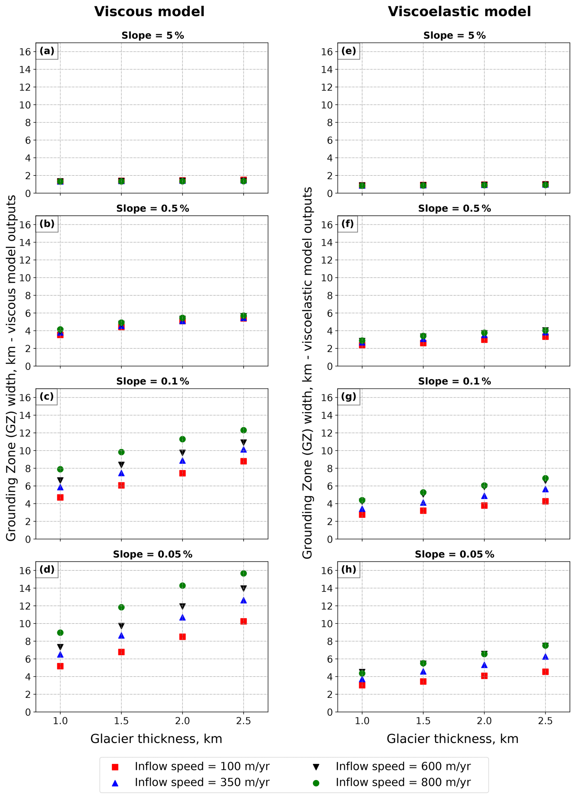
Figure 6 Dependence of the grounding zone width from the glacier thickness for inflow speeds of 100, 350, 600, and 800 m yr⁻¹ and bed slopes of 5 %, 0.5 %, 0.1 %, and 0.05 % for both viscous (a–d) and viscoelastic models (e–h). Corresponding bed slope is written above each panel, and the x axis of each panel shows the glacier thickness in kilometers, while the y axis shows the grounding zone width. Each panel contains four sets of values, colored based on the model inflow speed.

4.2.3 Impact of bed slope on grounding zone extent

Figure 7a and b present the grounding zone width obtained for the viscous and viscoelastic models, respectively, where the grounding zone values, indicated for different glacier thicknesses, are obtained by averaging the grounding zones for the same thickness across varying inflow speeds. Horizontal lines associated with the modeled grounding zones, in Fig. 7a and b, represent the range of modeled grounding zone width values as a function of ice speed for a given ice thickness. In both models, grounding zone width increases as the bedrock slope decreases, indicating that the relationship between glacier bed slope and grounding zone width follows an inverse power law (dotted lines in Fig. 7a and b). The steepest rate of decay is observed for the thinnest glaciers (1 km), which are associated with the narrowest grounding zones. The shallowest power law applies to the thickest glaciers (2.5 km), resulting in the widest grounding zones.

The grounding zone width values from the viscoelastic model (GZ_VE) plotted against the outputs from the viscous model (GZ_V) reveal a linear relationship: ${\mathrm{GZ}}_{\mathrm{VE}}=\mathrm{0.49}\cdot {\mathrm{GZ}}_{\mathrm{V}}+\mathrm{0.47}$, with a coefficient of determination (R²) of 0.97 (Fig. 7d). Consequently, for any combination of bedrock slope, glacier thickness, and ice inflow speed, the grounding zone width obtained from the viscoelastic model is nearly half that of the grounding zone width calculated by the viscous model on shorter timescales.

4.3 Evaluation of model performance using DInSAR grounding zone measurements

Figure 7c shows the superimposed outputs of the viscous and viscoelastic models alongside the DInSAR grounding zone measurements over MU, TOT, and REN glaciers. The dashed lines, outlining the models' domains, are shown in Fig. 7a, b, and c, while their equations are provided in Fig. 7a and b with the corresponding standard error of regression (S). The models' domains, shown in Fig. 7c in pink for the viscous model and in green for the viscoelastic model, were determined using the function $\mathit{\alpha }=a\cdot {\mathrm{GZ}}^b+c$, where α is the input bed slope; GZ is the modeled grounding zone; and a, b, and c are the fitting coefficients obtained through the least-squares fit of the model outputs in Fig. 7a and b. For each model, the upper domain boundary was established by fitting the largest modeled grounding zone outputs for each slope, while the lower domain boundary was defined by fitting the smallest modeled grounding zone outputs for each slope. The standard error of regression (S) is 0.12 and 0.16 for the upper and lower viscous domain boundaries, respectively, and 0.08 and 0.07 for the upper and lower viscoelastic domain boundaries, respectively. Therefore, the power law function $\mathit{\alpha }=a\cdot {\mathrm{GZ}}^b+c$ accurately represents not only the DInSAR-derived grounding zone measurements (Fig. S3), but also the models' output ranges.

To determine the models' accuracy, we measure the percentage of DInSAR measurements that fall inside the domain of a corresponding model. Disregarding the measurements error bars, only ∼ 29 %, ∼ 0 %, and ∼ 9 % of TOT's, REN's, and MU's measurements, respectively, fall into the viscous model's domain. Meanwhile, ∼ 88 % of TOT, 90 % of REN, and ∼ 82 % of MU measurements (not accounting for the measurements errors) are successfully accommodated by the viscoelastic model. When including measurement errors, the model performance improves (Table S7). For the viscous model, the percentage of successfully modeled measurements increases from ∼ 29 % to ∼ 65 % for TOT, from ∼ 0 % to ∼ 47 % for REN, and from ∼ 9 % to ∼ 82 % for MU. For the viscoelastic model, this performance improvement is evident in the following notable expansions: from ∼ 90 % to ∼ 100 % for REN, from ∼ 82 % to ∼ 100 % for MU, and remaining consistently at ∼ 88 % for TOT. Overall, considering all three glaciers and all profiles, the viscous model achieves approximately 12 % accuracy without measurement error bars and 70 % accuracy with them, while the viscoelastic model achieves around 86 % accuracy without error bars and 97 % accuracy with them. Therefore, considering all the profiles and the measurement error bars, the viscoelastic model outperforms the viscous model by ∼ 28 %. However, without error bars, the viscoelastic model outperforms the viscous model by ∼ 74 %. This finding underscores the critical importance of incorporating the elastic component in Navier–Stokes-based fluid glacier formulations for representing tidally induced grounding zone migrations.

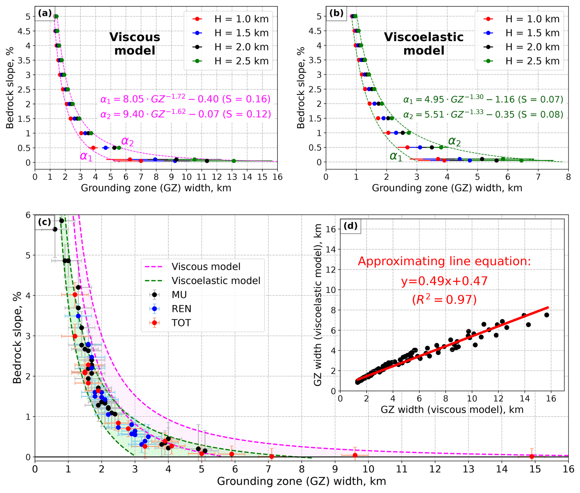
Figure 7 Modeling results of (a) viscous and (b) viscoelastic models, averaged by the thickness values, with pink and green outlines corresponding to maximum and minimum grounding zone (GZ) values for the same thickness but different inflow speeds. (c) Comparison of the modeling results (pink and green areas) with the DInSAR grounding zone measurements. (d) Correlation plot of the modeling results. Dotted green and pink lines are the same in panels (a), (b), and (c), while their equations are provided in panels (a) and (b).

5 Discussion

5.1 Grounding zone width dependence as a function of input parameters

Our models show that the grounding zone widens as the bed slope becomes shallower, following a nonlinear relationship. This model-derived finding is consistent with our data as well as with previous observational studies (Chen et al., 2023; Milillo et al., 2017, 2019, 2022). Furthermore, both our models and data indicate that wider grounding zones are found where glaciers are thicker, with a linear relationship observed (Fig. 8a and b). This observation can be associated with the increase in the flexural wavelength of ice when its thickness increases (Freer et al., 2023). For thicker ice, the same tidal amplitude affects a larger horizontal distance, leading to a broader grounding zone. This effect is more pronounced on shallow slopes, where the tidal amplitude influences a larger area. Glacier velocity significantly impacts grounding zone width for bed slopes below 0.1 % due to the increase in elastic stresses with faster glacier flow (Christmann et al., 2021). As a result, the elastic stress of fast-flowing glaciers on shallow slopes is higher than that of slower-moving glaciers, making the former more sensitive to thickness changes and supporting our observations (Fig. 8c). As shown in Eq. (44), a 1 m amplitude semidiurnal tide (12 h period) was used to simulate the tidal behavior of the studied glaciers. It should be noted that our DInSAR grounding line measurements rely on a single set of tidal observations (high and low tide) for each glacier. While these measurements do not always cover the full tidal range, they consistently capture a differential tidal variation of approximately 1 m (Table S2).

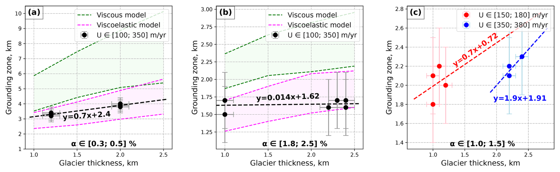
Figure 8 Relationship between glacier thickness and DInSAR-derived grounding zone width. (a) DInSAR measurements of grounding zone width (black dots) conducted along profiles characterized by bed slopes ranging from 0.3 % to 0.5 % and ice flow speeds from 100 to 350 m yr⁻¹. The dashed black line shows the linear correlation between the ice thickness and DInSAR-derived grounding zones. (b) The black dots and the dashed line correspond to DInSAR measurements described by bed slopes ranging from 1.8 % to 2.5 % and ice flow speeds from 100 to 350 m yr⁻¹ and their respective linear approximation. The green and pink areas in (a) and (b) correspond to the grounding zones, calculated by the viscous and viscoelastic models, respectively, for the same range of bed slopes and flow speeds as the DInSAR measurements, where dashed pink and green lines connect the corresponding model outputs. (c) Grounding zone measurements over 1.0 % to 1.5 % bed slopes, described by [150, 180] and [350, 380] m yr⁻¹ ice flow speeds with corresponding linear approximations.

5.2 Role of elasticity

Using the viscous model for slopes not shallower than 2 % can result in overestimating grounding zone widths by up to 25 %. For slopes shallower than 2 %, the viscous model overestimates grounding zone widths by up to 100 % (Fig. 7c). The viscous model tends to overestimate the grounding zones compared to the viscoelastic model due to several key factors. The viscoelastic model incorporates both the viscous (fluid-like) and elastic (solid-like) properties of ice, whereas the viscous model neglects the elastic component. This elastic response is fundamental over the tidal timescales, as ice exhibits elastic behavior under short-term deformations, such as those caused by tidal forces (Sayag and Worster, 2011; Warburton et al., 2020). Moreover, for cyclic loading, such as the tidal flexure of ice shelves, repeated loading and unloading make elastic effects significant (MacAyeal et al., 2015; Reeh et al., 2003). Additionally, the viscoelastic model more accurately captures time-dependent behavior by accounting for not only both the immediate elastic response and the delayed viscous response, but also the stress relaxation, a process neglected by purely viscous models (Christmann et al., 2019; MacAyeal et al., 2015). Research studies (Marsh et al., 2014; Reeh et al., 2000, 2003; Wild et al., 2017) confirm our conclusions regarding the critical importance of both viscous and elastic components at tidal timescales as viscoelastic models provide a more accurate representation of tidal bending processes.

While viscous models may be adequate for modeling long-term ice sheet evolution, they fail to represent important short-term phenomena such as tidal motion, seasonal cycles, and calving processes, which require the consideration of elastic responses. On the other hand, purely elastic models rely on a crucial simplification: they ignore the internal ice flow within the glacier, treating the glacier as a solid beam. By incorporating the viscous and elastic components in series, known as the Maxwell model of viscoelasticity, both slow and rapid deformations are considered. However, the simple Maxwell model describes small deformations, whereas the deformations of our interest may extend up to 50 % of the glacier domain length. Therefore, we applied the upper-convected Maxwell model of viscoelasticity, which includes some geometrical nonlinearity and allows the modeling of significantly larger deformations compared to the simple Maxwell model. Building on this, Christmann et al. (2021) emphasize that incorporating both viscous and elastic components is essential for realistic glacier dynamics modeling. In their study, the elastic component is crucial for accurately capturing the physical processes within a glacier, as it accounts for elastic strains in areas with sliding-dominated flow or high vertical deformations (Christmann et al., 2021). A similar argument was made by Hunke and Dukowicz (1997), highlighting that the elastic properties of ice temporarily reduce the overall deformation caused by the viscous component, which explains why the purely viscous model always estimates a wider grounding zone compared to the viscoelastic model. Elastic deformation is a short-term, recoverable response, while viscous deformation is a slower process that dominates over longer timescales. In situations involving short-duration forces, the elastic response can mitigate, but not eliminate, the visible effects of viscous deformation, providing a temporary reduction in overall glacier strain. This further highlights the necessity of incorporating both components for accurate modeling.

6 Conclusions

This study provides a comprehensive analysis of tide-induced grounding line variations across TOT, MU, and REN glaciers in East Antarctica using both viscous and viscoelastic models. Our results emphasize the crucial role of ice elasticity in modeling grounding zone behavior, particularly for glaciers on shallow bed slopes. Given the 400 m uncertainty on DInSAR-based grounding zone width measurements, the viscoelastic model consistently outperforms the viscous model, capturing 97 % of the grounding zone measurements when accounting for the measurement error. Overall, both models can capture the rationally decaying relationship between grounding zone width (GZ) and bed slope (α), expressed as $\mathit{\alpha }=a\cdot {\mathrm{GZ}}^b+c$, where a, b, and c are fitting parameters. The main difference lies in the dimensionless relaxation parameter b, which is ∼ 24 % smaller for the viscoelastic model, allowing it to better capture the observed dataset behavior. The elastic component introduces a damping effect, temporarily limiting the overall deformation caused by the viscous component (Hunke and Dukowicz, 1997). During a short timescale, the elastic component acts as a buffer, reducing the impact of elastic deformation, especially during cyclic events such as tidal flexure. This effect helps the viscoelastic model to accurately capture short-term glacier deformations and tide-induced grounding zones. On average, the elastic component reduces the tidally induced grounding zone width by half, shielding the grounding zones from the infiltration of warm water that melts the glacier from below (Rignot et al., 2024), thereby promoting a stabilizing effect. Accounting for the DInSAR-derived grounding zone width measurements error, the viscous model may be applied for grounding zone widths of less than 1.5 km and slopes steeper than 3 %. For shallower slopes, using a viscous model may lead to a 100 % overestimation of the grounding zone width. These findings reinforce the need for incorporating both viscous and elastic components in short-term glacier models to improve the prediction of grounding zone dynamics.

Glacier thickness and velocity also influence the grounding zone width, with thicker glaciers and faster flow speeds contributing to wider grounding zones. Increased ice thickness extends the flexural wavelength, enlarging the area affected by tidal forces, while higher glacier velocities amplify elastic stresses, further expanding the grounding zone. These effects are especially pronounced on shallow bed slopes, where even small changes in thickness and velocity can lead to significant variations in grounding zone extent.

This research underscores the critical impact of glacier thickness, bed slope, and ice velocity on grounding zone width, with elastic stresses playing a key role in fast-flowing glaciers on shallow slopes. As climate change continues to influence polar regions, this modeling framework offers valuable insights for understanding and predicting grounding zone dynamics and their contributions to global sea level rise. Future research should focus on extending this model to include a broader range of glaciers and further refining the viscoelastic model, particularly in response to tidal cycles and seasonal variations. This would enhance the model's predictive capability and provide deeper insights into how different environmental factors influence glacier dynamics, improving forecasts of grounding zone behavior and their implications for sea level rise.