A quasi-one-dimensional ice mélange flow model based on continuum descriptions of granular materials

Field and remote sensing studies suggest that ice mélange influences glacier–fjord systems by exerting stresses on glacier termini and releasing large amounts of freshwater into fjords. The broader impacts of ice mélange over long timescales are unknown, in part due to a lack of suitable ice mélange flow models. Previous efforts have included modifying existing viscous ice shelf models, despite the fact that ice mélange is fundamentally a granular material, and running computationally expensive discrete element simulations. Here, we draw on laboratory studies of granular materials, which exhibit viscous flow when stresses greatly exceed the yield point, plug flow when the stresses approach the yield point, and exhibit stress transfer via force chains. By implementing the nonlocal granular fluidity rheology into a depth- and width-integrated stress balance equation, we produce a numerical model of ice mélange flow that is consistent with our understanding of well-packed granular materials and that is suitable for long-timescale simulations. For parallel-sided fjords, the model exhibits two possible steady-state solutions. When there is no calving of icebergs or melting of previously calved icebergs, the ice mélange is pushed down-fjord by the advancing glacier terminus, the velocity is constant along the length of the fjord, and the thickness profile is exponential. When calving and melting are included and treated as constants, the ice mélange evolves into another steady state in which its location is fixed relative to the fjord walls, the thickness profile is relatively steep, and the flow is extensional. For the latter case, the model predicts that the steady-state ice mélange buttressing force depends on the surface and basal melt rates through an inverse power-law relationship, decays roughly exponentially with both fjord width and gradient in fjord width, and increases with the iceberg calving flux. The buttressing force appears to increase with calving flux (i.e., glacier thickness) more rapidly than the force required to prevent the capsizing of full-glacier-thickness icebergs, suggesting that glaciers with high calving fluxes may be more strongly influenced by ice mélange than those with small fluxes.

1 Introduction

Ice mélange is an intrinsically granular material that is comprised of icebergs, brash ice, and sea ice packed together at the ocean surface. In some fjords, where iceberg productivity is high, ice mélange can persist year-round. In others, it forms for a few months in winter, when sea ice binds the iceberg clasts together, and then breaks apart each spring. Ice mélange is a highly heterogeneous material, with clast dimensions varying from meters to hundred of meters in both horizontal and vertical dimensions. The large vertical dimension of ice mélange suggests that some processes that are important for sea ice and river ice, such as ridging and rafting, are likely unimportant for the flow of ice mélange.

Previous work has established that glacier advance between major calving events can result in the formation of an ice mélange wedge that flows quasi-statically and that exerts a force per unit width on the glacier terminus on the order of 10⁷ N m⁻¹ (Robel, 2017; Burton et al., 2018; Amundson and Burton, 2018). This load may be sufficient to inhibit calving and capsizing of new icebergs (e.g., Amundson et al., 2010; Krug et al., 2015; Bassis et al., 2021; Crawford et al., 2021; Schlemm et al., 2022), which is supported by studies that have linked breakup of a seasonal ice mélange wedge to the onset of calving in early summer (Cassotto et al., 2015; Bevan et al., 2019; Xie et al., 2019; Joughin et al., 2020). In locations where ice mélange persists year-round, it appears to remain sufficiently strong to influence the timing and seasonality of calving events (Wehrlé et al., 2023). Terrestrial radar data indicate that ice mélange flow becomes incoherent at the grain scale in the hours preceding major calving events (Cassotto et al., 2021), suggesting a weakening of the ice mélange, and that dynamic jamming occurs once an iceberg calves into the fjord (Peters et al., 2015).

Recent work has demonstrated that icebergs are also important sources of freshwater in fjords (Enderlin et al., 2016, 2018; Moon et al., 2017; Mortensen et al., 2020), especially during winter, and that this distributed release of freshwater has implications for fjord circulation and submarine melting of glacier termini. The presence of icebergs not only tends to freshen and cool fjords, but also helps to enhance estuarine circulation and drive warm water into fjords, where it comes into contact with and melts glacier termini (Davison et al., 2020). Icebergs additionally create complex flow pathways and tend to decrease the velocity of subsurface waters (Hughes, 2022).

The conclusion of many studies is that there is a strong need for an ice mélange model that is consistent with its granular nature and that can be mechanically and thermodynamically coupled to the glacier–ocean system. Previous modeling attempts have used discrete element models (Robel, 2017; Burton et al., 2018), modified existing ice shelf models (Pollard et al., 2018), incorporated sparse icebergs into sea ice models (Vaňková and Holland, 2017; Kahl et al., 2023), or used simple parameterizations (Schlemm and Levermann, 2021). Here we develop a depth-integrated ice mélange flow model that uses the nonlocal granular fluidity rheology (Henann and Kamrin, 2013), which has been developed from experiments of granular materials and that has successfully described a variety of granular flows. In order to investigate the basic behavior of the model and to expedite development of coupled glacier–ocean–mélange models, we convert the model into a quasi-one-dimensional model by separately parameterizing the longitudinal and shear stresses and then integrating across the fjord. This approach closely mimics one that is commonly used for developing flow line models for ice shelves, as does the numerical implementation of the model. Thus, this study provides a framework by which realistic models of ice mélange can be incorporated into coupled glacier–ocean models.

2 Model description

Following recent advances in granular mechanics, we treat ice mélange as a continuum whose behavior is described by a viscoplastic rheology. Although the rheology is more complicated than the power-law rheology typically used for modeling glacier flow (Cuffey and Paterson, 2010), our model setup is similar to that of the shallow shelf approximation (SSA). After subtracting the static pressure (modified to include the presence of water in between icebergs) from the stress tensor, we vertically integrate the stress balance equations and incorporate a depth-averaged form of the nonlocal granular fluidity rheology (Henann and Kamrin, 2013). The result is two horizontal stress balance equations, which we refer to as the nonlocal shallow mélange approximation. Future work will implement these two-dimensional equations in the finite-element method in order to model flow through complex geometries.

Here, to expedite implementation into coupled glacier–ocean–mélange models and to explore the basic model couplings, we width-integrate the model to produce a quasi-one-dimensional model (Fig. 1). A fundamental difference from analogous ice shelf models is that the description of the nonlocal granular fluidity rheology contains a second-order partial differential equation, which means that the rheology cannot be directly substituted into the stress balance equation(s) or be used to produce a simple parameterization of the lateral shear stress. As a result, the model contains five highly coupled equations that describe the ice mélange velocity, thickness, fluidity, length, and lateral shear stress. For comparison, the ice sheet–ice shelf model of Schoof (2007) only contains equations for the velocity, thickness, and length. Similarly to Schoof (2007), the equations are discretized using finite differences with a fully implicit time step and a moving grid that stretches from the glacier terminus to the end of the ice mélange. Material enters the domain through calving of icebergs, and icebergs smaller than the characteristic iceberg size are removed from the end of the domain. The velocity at the upstream boundary depends on the glacier terminus velocity and iceberg calving rate, while the velocity gradient at the downstream boundary is set to 0 to prevent deformation below the grain scale. The model equations are then solved simultaneously through a minimization procedure. A list of model variables is included in Appendix D.

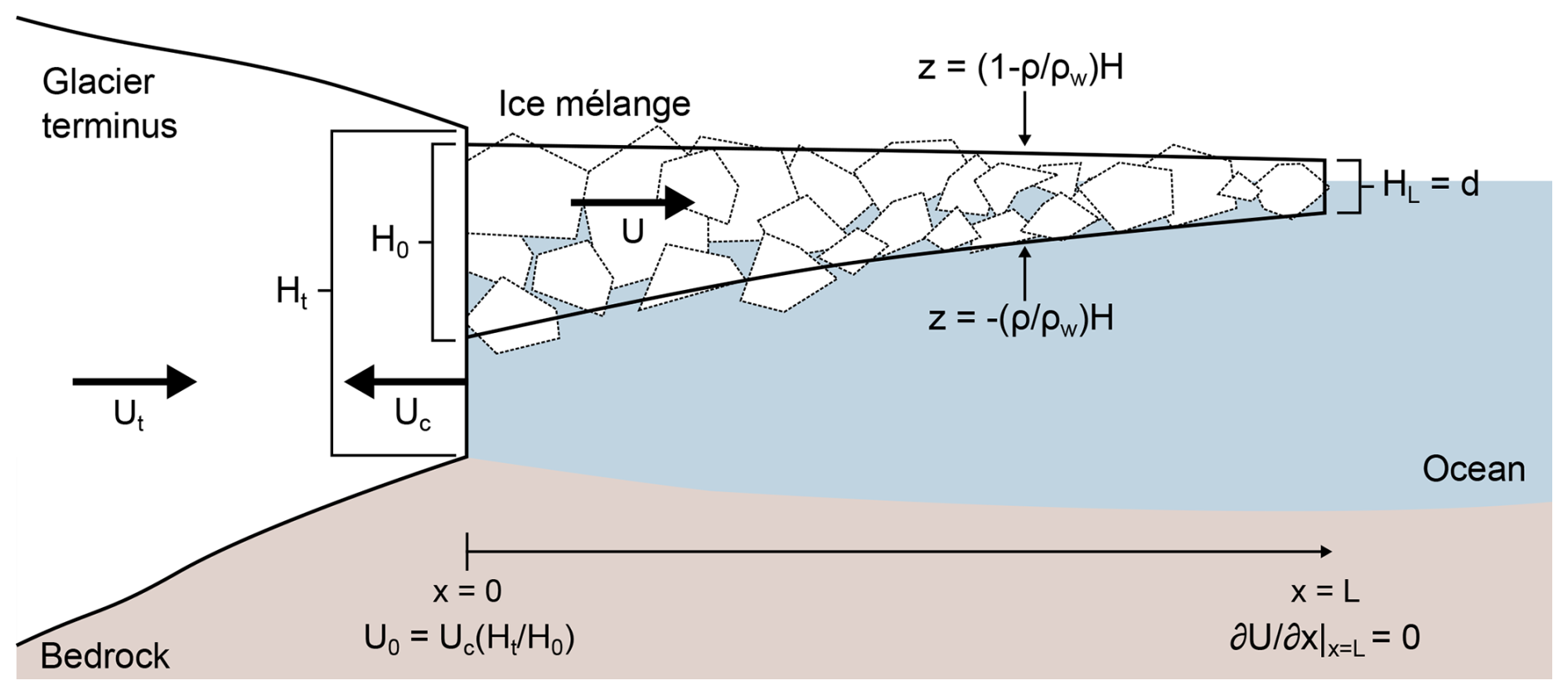
Figure 1 Schematic of the quasi-one-dimensional flow model indicating some of the key variables and boundary conditions.

2.1 Depth-integrated flow equations

We start by defining the strain rate and effective strain rate as ${\dot{\mathit{\epsilon }}}_{ij}=\mathrm{1}/\mathrm{2}(\partial u_i/\partial x_j+\partial u_j/\partial x_i)$ and ${\dot{\mathit{\epsilon }}}_e=({\dot{\mathit{\epsilon }}}_{ij}{\dot{\mathit{\epsilon }}}_{ij}/\mathrm{2}{)}^{\mathrm{1}/\mathrm{2}}$, where $\mathit{u}=\langle u,v,w\rangle$ and $\mathit{x}=\langle x,y,z\rangle$ are the velocity and position vectors. We use the Cauchy stress tensor, σ_ij=σ_ji, with the convention that positive stresses are extensional. In order to simplify depth integration of the equations of motion (see van der Veen and Whillans, 1989), we partition the stress tensor into tectonic stresses R_ij and the granular static pressure $\stackrel{\mathrm{̃}}{p}$ by setting ${\mathit{\sigma }}_{ij}=R_{ij}-\stackrel{\mathrm{̃}}{p}{\mathit{\delta }}_{ij}$, where δ_ij is the Kronecker delta. We assume that the ice mélange is tightly packed and incompressible (${\dot{\mathit{\epsilon }}}_{kk}=\mathrm{0}$), is at flotation, and is evolving slowly enough for acceleration to be neglected. Consequently, the model is best suited for simulating ice mélange behavior in fjords where it persists year-round or for winter conditions in fjords where it forms seasonally. Further modifications would be required to model rapid flow associated with calving events or complete dispersal of ice mélange in summer. For well-packed ice mélange, the inertial number (the ratio of inertial forces to confining forces; GDR MiDi, 2004) is typically very small ($<{\mathrm{10}}^{-\mathrm{5}}$; see Amundson and Burton, 2018), which places it well within the quasi-static regime. Under steady flow conditions, the equations of motion are then

$$\begin{array}{}\text{(1)}& {\displaystyle \frac{\partial {\mathit{\sigma }}_{ij}}{\partial x_j}}=\mathit{\rho }{g}_{\mathrm{eff}}{\mathit{\delta }}_{iz},\end{array}$$

where ρ is the material density and g_eff is the effective gravity that is given by

$$\begin{array}{}\text{(2)}& g_{\mathrm{eff}}=\left\{\begin{array}{ll}g& z\ge \mathrm{0}\\ \left(\mathrm{1}-\frac{{\mathit{\rho }}_{\mathrm{w}}}{\mathit{\rho }}\right)g& z<\mathrm{0},\end{array}\right.\end{array}$$

with ρ_w being the density of water, g being the gravitational acceleration, and z=0 corresponding to sea level. This formulation differs from that used to derive the shallow shelf approximation because seawater fills void spaces within ice mélange, and thus the static pressure does not depend solely on the weight of the overlying ice. The static pressure is found by noting that $\mathrm{d}\stackrel{\mathrm{̃}}{p}/\mathrm{d}z=-\mathit{\rho }{g}_{\mathrm{eff}}$ and $\stackrel{\mathrm{̃}}{p}=\mathrm{0}$ at the top and bottom of the ice mélange. Integrating from z to the surface (i.e., $z=(\mathrm{1}-\mathit{\rho }/{\mathit{\rho }}_{\mathrm{w}})H$) results in

$$\begin{array}{}\text{(3)}& \stackrel{\mathrm{̃}}{p}\left(z\right)=\left\{\begin{array}{ll}\mathit{\rho }g\left[\left(\mathrm{1}-\frac{\mathit{\rho }}{{\mathit{\rho }}_{\mathrm{w}}}\right)H-z\right]& z\ge \mathrm{0}\\ \mathit{\rho }g\left(\mathrm{1}-\frac{\mathit{\rho }}{{\mathit{\rho }}_{\mathrm{w}}}\right)\left(H+\frac{{\mathit{\rho }}_{\mathrm{w}}}{\mathit{\rho }}z\right)& z<\mathrm{0},\end{array}\right.\end{array}$$

where H is the ice mélange thickness.

Hughes (2022) modeled the flow of water through and beneath ice mélange and found that the drag force per unit width is 1–10 kN m⁻¹, which is 1 to 2 orders of magnitude smaller than the drag forces due to lateral shear that we calculate in our model. We therefore neglect basal shear stresses but note that future efforts may need to include them in order to model fjords in which ice mélange does not remain well packed or persist year-round. A consequence of neglecting basal shear stresses is that vertical shear is negligible, and therefore velocities, strain rates, and tectonic stresses do not vary with depth. Thus, after partitioning the stress tensor, vertical integration of the momentum equations leads to

$$\begin{array}{}\text{(4)}& \begin{array}{rl}& {\displaystyle \frac{\partial }{\partial x}}\left(H{R}_{xx}\right)+{\displaystyle \frac{\partial }{\partial y}}\left(H{R}_{xy}\right)=\mathrm{2}H{\displaystyle \frac{\partial \stackrel{\mathrm{̃}}{P}}{\partial x}}\\ & {\displaystyle \frac{\partial }{\partial y}}\left(H{R}_{yy}\right)+{\displaystyle \frac{\partial }{\partial x}}\left(H{R}_{xy}\right)=\mathrm{2}H{\displaystyle \frac{\partial \stackrel{\mathrm{̃}}{P}}{\partial y}},\end{array}\end{array}$$

where

$$\begin{array}{}\text{(5)}& \stackrel{\mathrm{̃}}{P}={\displaystyle \frac{\mathrm{1}}{\mathrm{2}}}\mathit{\rho }g\left(\mathrm{1}-{\displaystyle \frac{\mathit{\rho }}{{\mathit{\rho }}_{\mathrm{w}}}}\right)H\end{array}$$

is the depth-averaged granular static pressure.

The depth-averaged deviatoric stress is defined as ${\stackrel{\mathrm{‾}}{\mathit{\sigma }}}_{ij}^{\prime }={\stackrel{\mathrm{‾}}{\mathit{\sigma }}}_{ij}+P{\mathit{\delta }}_{ij}$, where the bar refers to depth-averaged values and $P=-({\stackrel{\mathrm{‾}}{\mathit{\sigma }}}_{xx}+{\stackrel{\mathrm{‾}}{\mathit{\sigma }}}_{yy}+{\stackrel{\mathrm{‾}}{\mathit{\sigma }}}_{zz})/\mathrm{3}$ is the depth-averaged isometric pressure. As with the tectonic stresses, the deviatoric stresses do not vary with depth in our model, and therefore ${\stackrel{\mathrm{‾}}{\mathit{\sigma }}}_{ij}^{\prime }={\mathit{\sigma }}_{ij}^{\prime }$. By vertically integrating the tectonic stress and comparing the result to the deviatoric stress (following van der Veen, 2013), we find that

$$\begin{array}{}\text{(6)}& R_{ij}={\mathit{\sigma }}_{ij}^{\prime }-\left(P-\stackrel{\mathrm{̃}}{P}\right){\mathit{\delta }}_{ij}.\end{array}$$

When $i=j=z$, Eq. (6) can be rewritten to show that

$$\begin{array}{}\text{(7)}& \left(P-\stackrel{\mathrm{̃}}{P}\right)={\mathit{\sigma }}_{zz}^{\prime }-R_{zz}=-{\mathit{\sigma }}_{xx}^{\prime }-{\mathit{\sigma }}_{yy}^{\prime }-R_{zz}.\end{array}$$

Due to its granular nature, ice mélange will not flex like ice shelves, which are often close to being in hydrostatic equilibrium except near their grounding lines. We therefore assume that bridging effects are negligible (i.e., that the weight of the ice mélange is locally supported by seawater) and therefore R_zz=0. Thus Eq. (6) becomes

$$\begin{array}{}\text{(8)}& R_{ij}={\mathit{\sigma }}_{ij}^{\prime }+({\mathit{\sigma }}_{xx}^{\prime }+{\mathit{\sigma }}_{yy}^{\prime }){\mathit{\delta }}_{ij}.\end{array}$$

Following Amundson and Burton (2018), we assume a depth-integrated viscoplastic rheology for granular materials:

$$\begin{array}{}\text{(9)}& {\mathit{\sigma }}_{ij}^{\prime }={\displaystyle \frac{\mathit{\mu }P}{{\dot{\mathit{ϵ}}}_e}}{\dot{\mathit{ϵ}}}_{ij},\end{array}$$

where μ is an effective coefficient of friction within the ice mélange that depends nonlinearly on the strain rate (see below). From Eq. (7) we see that $P=\stackrel{\mathrm{̃}}{P}+{\mathit{\sigma }}_{zz}^{\prime }$ (since R_zz=0), and therefore

$$\begin{array}{}\text{(10)}& {\mathit{\sigma }}_{ij}^{\prime }={\displaystyle \frac{\mathit{\mu }(\stackrel{\mathrm{̃}}{P}+{\mathit{\sigma }}_{zz}^{\prime })}{{\dot{\mathit{ϵ}}}_e}}{\dot{\mathit{ϵ}}}_{ij}.\end{array}$$

Setting $i=j=z$ and rearranging yields

$$\begin{array}{}\text{(11)}& {\mathit{\sigma }}_{zz}^{\prime }={\displaystyle \frac{\mathit{\mu }\stackrel{\mathrm{̃}}{P}{\dot{\mathit{ϵ}}}_{zz}}{{\dot{\mathit{ϵ}}}_e-\mathit{\mu }{\dot{\mathit{ϵ}}}_{zz}}}.\end{array}$$

Inserting Eq. (11) into Eq. (10) and simplifying results in

$$\begin{array}{}\text{(12)}& {\mathit{\sigma }}_{ij}^{\prime }={\displaystyle \frac{\mathit{\mu }\stackrel{\mathrm{̃}}{P}}{{\dot{\mathit{ϵ}}}_e-\mathit{\mu }{\dot{\mathit{ϵ}}}_{zz}}}{\dot{\mathit{ϵ}}}_{ij}={\displaystyle \frac{\mathit{\mu }\stackrel{\mathrm{̃}}{P}}{{\dot{\mathit{ϵ}}}_e+\mathit{\mu }\left({\dot{\mathit{ϵ}}}_{xx}+{\dot{\mathit{ϵ}}}_{yy}\right)}}{\dot{\mathit{ϵ}}}_{ij}.\end{array}$$

The tectonic stress is then found by inserting Eq. (12) into Eq. (8):

$$\begin{array}{}\text{(13)}& R_{ij}={\displaystyle \frac{\mathit{\mu }\stackrel{\mathrm{̃}}{P}}{{\dot{\mathit{ϵ}}}_e+\mathit{\mu }({\dot{\mathit{ϵ}}}_{xx}+{\dot{\mathit{ϵ}}}_{yy})}}\left[{\dot{\mathit{ϵ}}}_{ij}+\left({\dot{\mathit{ϵ}}}_{xx}+{\dot{\mathit{ϵ}}}_{yy}\right){\mathit{\delta }}_{ij}\right].\end{array}$$

Substituting Eq. (5) into Eq. (13) and the result into Eq. (4), dividing by $\mathit{\rho }g(\mathrm{1}-\mathit{\rho }/{\mathit{\rho }}_{\mathrm{w}})/\mathrm{2}$, and rearranging gives

$$\begin{array}{}\text{(14)}& \begin{array}{rl}& {\displaystyle \frac{\partial }{\partial x}}\left[{\displaystyle \frac{\mathit{\mu }{H}^{\mathrm{2}}}{{\dot{\mathit{ϵ}}}_e+\mathit{\mu }({\dot{\mathit{ϵ}}}_{xx}+{\dot{\mathit{ϵ}}}_{yy})}}(\mathrm{2}{\dot{\mathit{ϵ}}}_{xx}+{\dot{\mathit{ϵ}}}_{yy})\right]\\ & +{\displaystyle \frac{\partial }{\partial y}}\left[{\displaystyle \frac{\mathit{\mu }{H}^{\mathrm{2}}}{{\dot{\mathit{ϵ}}}_e+\mathit{\mu }({\dot{\mathit{ϵ}}}_{xx}+{\dot{\mathit{ϵ}}}_{yy})}}{\dot{\mathit{ϵ}}}_{xy}\right]=\mathrm{2}H{\displaystyle \frac{\partial H}{\partial x}}\\ & {\displaystyle \frac{\partial }{\partial y}}\left[{\displaystyle \frac{\mathit{\mu }{H}^{\mathrm{2}}}{{\dot{\mathit{ϵ}}}_e+\mathit{\mu }({\dot{\mathit{ϵ}}}_{xx}+{\dot{\mathit{ϵ}}}_{yy})}}(\mathrm{2}{\dot{\mathit{ϵ}}}_{yy}+{\dot{\mathit{ϵ}}}_{xx})\right]\\ & +{\displaystyle \frac{\partial }{\partial x}}\left[{\displaystyle \frac{\mathit{\mu }{H}^{\mathrm{2}}}{{\dot{\mathit{ϵ}}}_e+\mathit{\mu }({\dot{\mathit{ϵ}}}_{xx}+{\dot{\mathit{ϵ}}}_{yy})}}{\dot{\mathit{ϵ}}}_{xy}\right]=\mathrm{2}H{\displaystyle \frac{\partial H}{\partial y}}.\end{array}\end{array}$$

In viscoplastic granular rheologies, μ is a complex function of ${\dot{\mathit{ϵ}}}_e$. We adopt the nonlocal granular fluidity rheology of Henann and Kamrin (2013), which is derived from laboratory experiments that demonstrate viscous flow at high stress and plug flow at low stress. The rheology is nonlocal because it enables mesoscopic regions of yielding to cause elastic deformation in adjacent jammed regions, and it is particularly well suited for ice mélange because it has been developed from experiments of flows associated with low inertial numbers. The nonlocal granular fluidity rheology has successfully modeled a variety of granular flows, including flow down a rough plane (Kamrin and Henann, 2015), creep of intruders in low-stress regions (Henann and Kamrin, 2014), annular shear with various grain geometries and materials (Fazelpour et al., 2022), and silo clogging (Dunatunga and Kamrin, 2022), and it has also recently been applied to other geophysical systems (e.g., Damsgaard et al., 2020; Zhang et al., 2022).

In the nonlocal granular fluidity rheology, the effective coefficient of friction depends on the granular fluidity, g^′, which is a measure of how easily the material can flow for a given stress:

$$\begin{array}{}\text{(15)}& \mathit{\mu }\equiv {\displaystyle \frac{{\dot{\mathit{ϵ}}}_e}{g^{\prime }}}.\end{array}$$

The granular fluidity depends on local and distant stresses through the differential relation

$$\begin{array}{}\text{(16)}& {\mathrm{\nabla }}^{\mathrm{2}}{g}^{\prime }={\displaystyle \frac{\mathrm{1}}{{\mathit{\xi }}^{\mathrm{2}}}}\left(g^{\prime }-g_{\mathrm{loc}}^{\prime }\right),\end{array}$$

where ξ is the cooperativity length and $g_{\mathrm{loc}}^{\prime }$ is the local granular fluidity (i.e., the fluidity in the absence of flow or stress gradients). The local granular fluidity is based on experiments that suggest that granular materials behave like Bingham fluids (solid at low stresses and viscous at high stresses):

$$\begin{array}{}\text{(17)}& g_{\mathrm{loc}}^{\prime }=\left\{\begin{array}{ll}\sqrt{\frac{P}{\mathit{\rho }{d}^{\mathrm{2}}}}\frac{(\mathit{\mu }-{\mathit{\mu }}_{\mathrm{s}})}{\mathit{\mu }b}& \text{if}\mathit{\mu }>{\mathit{\mu }}_{\mathrm{s}}\\ \mathrm{0}& \text{if}\mathit{\mu }\le {\mathit{\mu }}_{\mathrm{s}},\end{array}\right.\end{array}$$

where b is a dimensionless constant, μ_s is the static yield coefficient, and the isometric pressure is related to the granular static pressure by $P=\stackrel{\mathrm{̃}}{P}{\dot{\mathit{ϵ}}}_e/({\dot{\mathit{ϵ}}}_e+\mathit{\mu }({\dot{\mathit{ϵ}}}_{xx}+{\dot{\mathit{ϵ}}}_{yy}\left)\right)$ (compare Eqs. 10 and 12). The Laplacian term in Eq. (16) spreads out the fluidity into regions where μ<μ_s (Kamrin and Koval, 2012) and allows for deformation in regions of low stress. The distance over which the fluidity spreads out is determined by the cooperativity length, which scales with grain size and diverges at the yield point (Bocquet et al., 2009; Kamrin and Henann, 2015):

$$\begin{array}{}\text{(18)}& \mathit{\xi }={\displaystyle \frac{Ad}{\sqrt{|\mathit{\mu }-{\mathit{\mu }}_{\mathrm{s}}|}}},\end{array}$$

where A is a dimensionless constant.

Substituting Eq. (15) into Eq. (14) yields

$$\begin{array}{}\text{(19)}& \begin{array}{rl}& {\displaystyle \frac{\partial }{\partial x}}\left[{\displaystyle \frac{H^{\mathrm{2}}}{g^{\prime }+{\dot{\mathit{ϵ}}}_{xx}+{\dot{\mathit{ϵ}}}_{yy}}}(\mathrm{2}{\dot{\mathit{ϵ}}}_{xx}+{\dot{\mathit{ϵ}}}_{yy})\right]\\ & +{\displaystyle \frac{\partial }{\partial y}}\left[{\displaystyle \frac{H^{\mathrm{2}}}{g^{\prime }+{\dot{\mathit{ϵ}}}_{xx}+{\dot{\mathit{ϵ}}}_{yy}}}{\dot{\mathit{ϵ}}}_{xy}\right]=\mathrm{2}H{\displaystyle \frac{\partial H}{\partial x}}\\ & {\displaystyle \frac{\partial }{\partial y}}\left[{\displaystyle \frac{H^{\mathrm{2}}}{g^{\prime }+{\dot{\mathit{ϵ}}}_{xx}+{\dot{\mathit{ϵ}}}_{yy}}}(\mathrm{2}{\dot{\mathit{ϵ}}}_{yy}+{\dot{\mathit{ϵ}}}_{xx})\right]\\ & +{\displaystyle \frac{\partial }{\partial x}}\left[{\displaystyle \frac{H^{\mathrm{2}}}{g^{\prime }+{\dot{\mathit{ϵ}}}_{xx}+{\dot{\mathit{ϵ}}}_{yy}}}{\dot{\mathit{ϵ}}}_{xy}\right]=\mathrm{2}H{\displaystyle \frac{\partial H}{\partial y}}.\end{array}\end{array}$$

Equation (19), along with the equations for g^′ (Eqs. 15–18), is analogous to the shallow shelf approximation. We therefore refer to Eq. (19) as the nonlocal shallow mélange approximation (NSMA). As with the shallow shelf approximation, the NSMA requires some regularization to prevent infinite viscosity.

2.2 Width-integrated flow equations and boundary conditions

To reduce Eq. (19) to a quasi-one-dimensional flow model, we adopt an approach from glacier flow modeling in which extension-dominated dynamics are used to characterize the longitudinal stresses and shear-dominated dynamics are used to characterize the shear stresses (Pegler, 2016). This approach allows for width integration of the flow equations and, importantly, asymptotes to the correct dynamics in extension- and shear-dominated regimes. Essentially, we assume that (i) flow is in the x direction and variations in width are small (i.e., $|\mathrm{d}W/\mathrm{d}x|\ll \mathrm{1}$; Pegler, 2016) so that v≈0 and ${\dot{\mathit{ϵ}}}_{yy}\approx \mathrm{0}$; (ii) the ice mélange thickness and longitudinal strain rates are uniform across the width of the fjord; and (iii) the granular fluidity in the longitudinal stress term (R_xx) is only a function of ${\dot{\mathit{ϵ}}}_{xx}$, while the granular fluidity in the shear stress term (R_xy) is only a function of ${\dot{\mathit{ϵ}}}_{xy}$.

Under these assumptions, integrating the x component of Eq. (19) across the fjord and dividing by the width W yields

$$\begin{array}{}\text{(20)}& {\displaystyle \frac{\partial }{\partial x}}\left[{\displaystyle \frac{H^{\mathrm{2}}}{g^x+{\dot{\mathit{ϵ}}}_{xx}}}{\dot{\mathit{ϵ}}}_{xx}\right]-{\displaystyle \frac{H^{\mathrm{2}}}{W}}{\mathit{\mu }}_{\mathrm{w}}{\left({\displaystyle \frac{{\dot{\mathit{ϵ}}}_{xy}}{{\dot{\mathit{ϵ}}}_e}}\right)}_{y=\mathrm{0}}=H{\displaystyle \frac{\partial H}{\partial x}},\end{array}$$

where g^x is used to indicate that the granular fluidity in the longitudinal stress term depends solely on ${\dot{\mathit{ϵ}}}_{xx}$, μ_w is the value of μ along the fjord walls, y is taken to be the distance from the near wall of the fjord, and due to symmetry the shear strain rates at y=0 and y=W have the same magnitude but opposite sign. Due to our assumptions, the y component of Eq. (19) does not affect flow in the x direction and can be ignored. The first and second terms in Eq. (20) characterize extension- and shear-dominated dynamics, respectively.

For shear-dominated flow, $({\dot{\mathit{ϵ}}}_{xy}/{\dot{\mathit{ϵ}}}_e){|}_{y=\mathrm{0}}=\mathrm{sgn}\left({\dot{\mathit{ϵ}}}_{xy}\right){|}_{y=\mathrm{0}}=\mathrm{sgn}\left(U\right)$, where U is the depth- and width-averaged velocity. Thus, combining and rearranging Eq. (20) gives the following one-dimensional stress balance equation:

$$\begin{array}{}\text{(21)}& {\displaystyle \frac{\partial }{\partial x}}\left[{\displaystyle \frac{H^{\mathrm{2}}}{g^x+(\partial U/\partial x)}}{\displaystyle \frac{\partial U}{\partial x}}\right]=H{\displaystyle \frac{\partial H}{\partial x}}+{\displaystyle \frac{H^{\mathrm{2}}}{W}}{\mathit{\mu }}_{\mathrm{w}}\mathrm{sgn}\left(U\right).\end{array}$$

Equation (21) is the key dynamical equation that is used to determine the ice mélange velocity along the length of the fjord. We use a reference frame that moves with the glacier terminus and define x=0 as being the glacier–ice mélange boundary. At this boundary, material flows into the domain at a rate determined by the iceberg calving flux. Conservation of mass dictates that the velocity there is given by

$$\begin{array}{}\text{(22)}& U_{\mathrm{0}}=U_{\mathrm{c}}{\displaystyle \frac{H_{\mathrm{t}}}{H_{\mathrm{0}}}},\end{array}$$

where subscript 0 refers to values at x=0, U_c is the calving rate, and H_t is the terminus thickness. We define the downstream end of the ice mélange (x=L) as being the point where the ice thins to the grain scale, d. At thicknesses less than the grain scale, the nonlocal granular fluidity rheology no longer applies. In order to prevent divergence for thicknesses less than the grain scale, we therefore require that the velocity gradient there is

$$\begin{array}{}\text{(23)}& {\left.{\displaystyle \frac{\partial U}{\partial x}}\right|}_{x=L}=\mathrm{0}.\end{array}$$

This downstream boundary condition is similar to regularizations used in sea ice models to prevent ice floes with free boundaries from spreading under their own weight (Hibler, 2001; Leppäranta, 2012).

The granular fluidity g^x is described by a simplified version of Eq. (16) in which g^′ and $g_{\mathrm{loc}}^{\prime }$ are replaced with g^x and $g_{\mathrm{loc}}^x$, ${\mathrm{\nabla }}^{\mathrm{2}}{g}^x={\partial }^{\mathrm{2}}{g}^x/\partial x^{\mathrm{2}}$, and ${\dot{\mathit{ϵ}}}_e=\left|{\dot{\mathit{ϵ}}}_{xx}\right|+{\mathit{\delta }}_{\dot{\mathit{ϵ}}}$. ${\mathit{\delta }}_{\dot{\mathit{ϵ}}}$ is a strain rate parameter that is used to regularize the granular fluidity equations in order to improve stability and efficiency. The regularization is applied when substituting μ (Eq. 24) into Eqs. (17) and (18) to ensure that the granular fluidity is always greater than 0. Other regularization schemes are possible (Chauchat and Médale, 2014); however, we have had success with this simple regularization scheme and therefore leave investigation of other schemes for future work. For boundary conditions we set $\partial g^x/\partial x=\mathrm{0}$ at $x=\mathrm{0},L$ following the recommendation of Henann and Kamrin (2013).

The value of μ_w in Eq. (21) is related to the width-averaged velocity relative to the fjord walls, which is given by $U+(U_{\mathrm{t}}-U_{\mathrm{c}})$, where U_t is the glacier terminus velocity and U_t−U_c is the rate of glacier terminus migration. In other words, the fjord walls move backward in our coordinate system, which is defined relative to the glacier terminus, at a rate given by U_t−U_c. For shear-dominated flow, integration of the x component of Eq. (19) from y=0 to y reveals that μ_w varies linearly across the fjord. By comparing the result to Eq. (20), we find that

$$\begin{array}{}\text{(24)}& \mathit{\mu }={\mathit{\mu }}_{\mathrm{w}}\left(\mathrm{1}-{\displaystyle \frac{\mathrm{2}y}{W}}\right)\end{array}$$

for $\mathrm{0}\le y\le W/\mathrm{2}$ (see also Amundson and Burton, 2018). Using Eq. (24), the local granular fluidity and cooperativity length can be readily calculated as functions of position for a given value of μ_w. The results are then inserted into the granular fluidity differential equation (Eq. 16), except that g^′ and $g_{\mathrm{loc}}^{\prime }$ are replaced with g^y and $g_{\mathrm{loc}}^y$ (to emphasize that the granular fluidity for shear-dominated flow depends only on ${\dot{\mathit{ϵ}}}_{xy}$) and ${\mathrm{\nabla }}^{\mathrm{2}}{g}^y={\partial }^{\mathrm{2}}{g}^y/\partial y^{\mathrm{2}}$. As before, we set $\partial g^y/\partial y=\mathrm{0}$ at both boundaries. The granular fluidity equation is then solved to determine g^y(y,μ_w). If the flow is in the positive x direction, then ${\dot{\mathit{ϵ}}}_e=(\partial U/\partial y)/\mathrm{2}$ and Eq. (15) can be rewritten as

$$\begin{array}{}\text{(25)}& {\displaystyle \frac{\partial u}{\partial y}}=\mathrm{2}\mathit{\mu }{g}^y=\mathrm{2}{\mathit{\mu }}_{\mathrm{w}}\left(\mathrm{1}-{\displaystyle \frac{\mathrm{2}y}{W}}\right)g^y(y,{\mathit{\mu }}_{\mathrm{w}}).\end{array}$$

The average velocity in the transect is found by integrating Eq. (25), which must equal the velocity in the bedrock reference frame:

$$\begin{array}{}\text{(26)}& U+U_{\mathrm{t}}-U_{\mathrm{c}}={\displaystyle \frac{\mathrm{2}}{W}}\underset{\mathrm{0}}{\overset{W/\mathrm{2}}{\int }}\underset{\mathrm{0}}{\overset{y}{\int }}\mathrm{2}{\mathit{\mu }}_{\mathrm{w}}\left(\mathrm{1}-{\displaystyle \frac{\mathrm{2}{y}^{\prime }}{W}}\right)g^y(y^{\prime },{\mathit{\mu }}_{\mathrm{w}})\mathrm{d}{y}^{\prime }\mathrm{d}y.\end{array}$$

Finally, the ice mélange geometry changes in response to melting, flow divergence, and dispersal of icebergs at x=L. The surface evolves according to the depth- and width-integrated mass continuity equation (van der Veen, 2013), in which

$$\begin{array}{}\text{(27)}& {\displaystyle \frac{\partial H}{\partial t}}=\dot{B}-{\displaystyle \frac{\mathrm{1}}{W}}{\displaystyle \frac{\partial }{\partial x}}\left(UHW\right),\end{array}$$

where $\dot{B}$ is the surface plus basal mass balance rate, and the length evolves so as to ensure that the thickness at the end of the ice mélange is always equal to the characteristic iceberg size.

2.3 Numerical implementation and stability considerations

The quasi-one-dimensional ice mélange flow model that we have developed depends on five variables: U, g^x, μ_w, H, and L. We determine these variables by simultaneously solving the width-integrated NSMA, granular fluidity, transverse velocity, and mass continuity equations (Eqs. 21, 16, 26, and 27) while also requiring that H_L=d. We use finite differences with a stretched coordinate system and a staggered grid for velocity and thickness. The mass continuity equation uses an implicit time-stepping scheme and an upwind scheme for discretization. Our numerical scheme, which closely mimics that of Schoof (2007), is described in detail in the Appendix.

The width-integrated NSMA is more computationally expensive than the analogous width-integrated SSA approximation for two reasons. First, the nonlocal granular fluidity rheology introduces additional nonlinear differential equations that must be solved as part of the iteration procedure, essentially doubling the number of unknowns. Second, because ice mélange tends to be considerably thinner than its parent glacier, ice mélange velocities must be several times higher than glacier terminus velocities in order to balance the ice flux into the fjord. This latter effect becomes particularly critical if ice mélange thins to close to its characteristic iceberg size.

For example, although we are using an implicit scheme, we find that the CFL (Courant–Friedrichs–Lewy) condition ($\mathrm{\Delta }t\le C_{\max }\mathrm{\Delta }x/U$) is a useful metric for determining appropriate time steps that maintain numerical stability. From our experience, C_max=1 provides good stability across a range of parameter choices and model states, although this is not a strict requirement. At x₀, the ice mélange velocity is $U_{\mathrm{0}}=U_c{H}_{\mathrm{t}}/H_{\mathrm{0}}$ (Eq. 22). Thus the CFL condition at x₀ can be expressed as

$$\begin{array}{}\text{(28)}& \mathrm{\Delta }t\le {\displaystyle \frac{\mathrm{\Delta }x{H}_{\mathrm{0}}}{U_c{H}_{\mathrm{t}}}}.\end{array}$$

For thick ice mélange (H₀≈H_t), with a calving rate of 6000 m a⁻¹, a terminus thickness of H_t=600 m, and a grid spacing of 500 m, Δt<0.09 a. However if the ice mélange approaches the characteristic iceberg size, for example $H_{\mathrm{0}}\approx d=\mathrm{25}$ m, then $\mathrm{\Delta }t<\mathrm{4}\times {\mathrm{10}}^{-\mathrm{3}}$ a (assuming similar grid spacing). In reality, higher velocities may occur farther down-fjord, necessitating shorter time steps. Since our model uses a moving grid and the ice mélange thickness and length may vary significantly over seasonal timescales, we recommend using short time steps or an adaptive time step in prognostic simulations.

2.4 Ice mélange buttressing force

Although we do not model glacier flow in this paper, we do assess the impact of model parameters, glacier fluxes, melt rates, and fjord geometry on the buttressing force that ice mélange exerts on glacier termini, which is given by $(-\mathrm{HW}{\mathit{\sigma }}_{xx}){|}_{x_{\mathrm{0}}}$. The force imposed on a glacier terminus (per unit width) due to the presence of ice mélange is therefore

$$\begin{array}{}\text{(29)}& F/W={\left(-H{R}_{xx}+H\stackrel{\mathrm{̃}}{P}\right)}_{x_{\mathrm{0}}}.\end{array}$$

Substituting in the nonlocal granular fluidity rheology yields

$$\begin{array}{}\text{(30)}& F/W={\left(-{\displaystyle \frac{\mathrm{2}H\stackrel{\mathrm{̃}}{P}{\dot{\mathit{ϵ}}}_{xx}}{g^x+{\dot{\mathit{ϵ}}}_{xx}}}+H\stackrel{\mathrm{̃}}{P}\right)}_{x_{\mathrm{0}}}.\end{array}$$

In the limit that $\partial U/\partial x\to \mathrm{0}$, $F/W$ scales with the thickness squared, $H_{\mathrm{0}}^{\mathrm{2}}$.

3 Model results

3.1 Steady-state and quasi-static profiles

We begin exploring the model behavior by investigating the impact of model parameters and forcings on steady-state profiles. The model is capable of producing two types of steady-state solutions: there is one in which material is continuously flowing through the ice mélange domain and the geometry is steady in the bedrock reference frame, and there is one in which no material enters or leaves the ice mélange and the geometry is steady in a reference frame that moves down-fjord with the glacier terminus and the velocity is constant ($\partial U/\partial x=\mathrm{0}$). We refer to these two states as the “steady-state” and “quasi-static” regimes. We focus primarily on the steady-state regime as the quasi-static regime has already been analyzed in some detail in Amundson and Burton (2018).

Figure 2 Steady-state (solid curves) and quasi-static (dashed curves) profiles. (a–d) Longitudinal profiles of velocity, thickness, granular fluidity, and limit of internal friction along the fjord walls. (e) Transverse velocity profiles at various fractions χ of the distance along the ice mélange. For the steady-state simulation, $U_{\mathrm{t}}=U_{\mathrm{c}}=\mathrm{6000}$ m a⁻¹, H_t=600 m, W=4000 m, $\dot{B}=-\mathrm{0.6}$ m d⁻¹, d=25 m, μ_s=0.3, A=0.5, and $b=\mathrm{1}\times {\mathrm{10}}^{\mathrm{4}}$. Longitudinal coordinates are relative to the glacier terminus.

To produce steady-state profiles, we set the terminus velocity and calving rate to be constant and equal to each other and we set the surface mass balance rate equal to a constant. We then run prognostic simulations until the ice mélange length and thickness are no longer changing with time ($\mathrm{d}L/\mathrm{d}t=\mathrm{0}$ and $\partial H/\partial t=\mathrm{0}$). The approach that we adopt differs from that of Amundson and Burton (2018), in which we derived an expression for steady-state profiles in the quasi-static limit, in several important ways. Here (i) we do not set the calving and melt rates equal to 0, (ii) we do not require μ_w to be constant but instead solve for it, (iii) we allow for variable width, and (iv) the ice mélange length is not specified a priori but rather is determined by the balance of the inflow and melt rates. We then turn off calving and melting and allow the ice mélange to evolve into a new steady-state in order to demonstrate the changes in flow and geometry that occur during the transition from the steady-state regime to the quasi-static regime.

Example steady-state and quasi-static profiles are shown in Fig. 2. Velocities increase in the down-fjord direction in the steady-state scenario (solid lines in Fig. 2), which, when combined with surface and basal melting, leads to a relatively large thickness gradient. The extensional flow is also associated with an increase in μ_w in the down-fjord direction. Once calving and melting are turned off, the ice mélange evolves toward the quasi-static limit (dashed lines in Fig. 2). The velocities drop because there is no longer a flux of new material into the ice mélange and the icebergs are simply pushed at the rate of glacier terminus advance. Consequently the shear stresses decrease, which is reflected in a decrease in μ_w. The reduction in shear stresses and lack of surface or basal melting allow the ice mélange to thin and spread outward. At the quasi-static limit, the ice mélange has a roughly exponential thickness profile and μ_w is spatially constant. In Amundson and Burton (2018), we assumed that μ_w is a constant in the quasi-static limit and showed that this leads to a roughly exponential thickness profile; here we see it arise naturally through the momentum and mass continuity equations in a manner that is consistent with our prior assumptions.

3.1.1 Sensitivity to model parameters

The nonlocal granular fluidity rheology depends on several parameters that must be specified: the characteristic iceberg size d, dimensionless constants b and A (described below), and the static yield coefficient μ_s. For default values we have selected d=25 m, $b=\mathrm{1}\times {\mathrm{10}}^{\mathrm{4}}$, A=0.5, and μ_s=0.3, which produces thickness and velocity profiles that are roughly consistent with observations from Sermeq Kujalleq (Jakobshavn Isbræ), Helheim Glacier, and Kangerlussuaq Glacier (e.g., Foga et al., 2014; Amundson and Burton, 2018; Bevan et al., 2019; Xie et al., 2019). Here, we provide some context for our selection of default values and explore how adjusting these parameters affects the steady-state model behavior (refer to Fig. 3 throughout this section).

• The characteristic iceberg size influences the local granular fluidity (Eq. 17), the cooperativity length (Eq. 18), and the ice mélange extent (since the end of the domain is defined as being where H=d). Ice mélange is a highly heterogeneous material, with iceberg dimensions ranging from meters to hundreds of meters. Several studies indicate that the iceberg area (in map view) follows power-law size distributions, $p\left(a\right)\propto a^{-\mathit{\alpha }}$, with α ranging from 2.1–3.4 (e.g., Enderlin et al., 2016; Sulak et al., 2017; Kirkham et al., 2017; Kaluzienski et al., 2023). Power-law distributions require a minimum size threshold. Using a minimum area of 10 m² gives median and mean iceberg areas of about 13–18 m² and 17–110 m² (see Eqs. 6 and 8 in Kaluzienski et al., 2023), resulting in a characteristic diameter on the order of 4–10 m. It is unclear, however, how iceberg heterogeneity affects ice mélange flow or if there is a controlling iceberg size. Nonetheless, we find that decreasing the iceberg size causes the ice mélange to become weaker (more fluid; Fig. 3c) by both increasing the local granular fluidity and decreasing the cooperativity length; consequently, a smaller characteristic iceberg size leads to faster (Fig. 3a, e), thinner, and longer ice mélange (Fig. 3b).

• The dimensionless constant b is given by the ratio of the range of effective friction coefficients to the inertial number (see Kamrin and Henann, 2015), which is itself a function of grain size, characteristic strain rate, and pressure. These values are poorly constrained for ice mélange at present. Using typical values, we find that b is likely in the range of 10⁴–10⁶. b only affects the local granular fluidity (Eq. 17), and as such its impact on model behavior is more transparent than that of iceberg size. Increasing b reduces the local granular fluidity, making the ice mélange stiffer (less fluid; Fig. 3c) and leading to thicker and longer ice mélange (Fig. 3b) and lower velocities (Fig. 3a, e).

• The dimensionless constant A affects the cooperativity length (Eq. 18) and is thought to be of order 1; fitting to laboratory experiments and discrete element simulations suggests that A equals 0.5 for glass beads and 0.9 for stiff disks (Henann and Kamrin, 2013; Kamrin and Koval, 2014). For our simulations, using values of A=0.5 gives cooperativity lengths of a few kilometers in the longitudinal direction. Changing A does not have much impact on our results other than changing the curvature of the transverse velocity profiles (Fig. 3e).

• Lastly, the static yield coefficient determines the stress at which the ice mélange will begin to flow (Eqs. 17). Reducing the yield coefficient causes the ice mélange to deform more easily (Fig. 3c) and become thinner and shorter (Fig. 3b).

Determining appropriate model parameters that are able to describe ice mélange flow across a range of forcings and fjord geometries remains a major task. The default parameters that we have selected produce ice mélange geometries and velocity profiles that appear to be roughly consistent with field observations (e.g., see figures in Amundson and Burton, 2018; Bevan et al., 2019; and Xie et al., 2019). Adjusting any of the parameters appreciably from our default parameters will likely require modifying one or more additional parameters in order to produce profiles that are not too thin or too thick. For example, we can also produce similar profiles if we reduce the static yield coefficient but only if we increase b appropriately.

Figure 3 Steady-state profiles for various model parameter choices. For all simulations, $U_{\mathrm{t}}=U_{\mathrm{c}}=\mathrm{6000}$ m a⁻¹, $\dot{B}=-\mathrm{0.6}$ m d⁻¹, H_t=600 m, and W=4000 m. (a–d) Longitudinal profiles of velocity, thickness, granular fluidity, and limit of internal friction along the fjord walls. (e) Transverse velocity profiles at the ice mélange midpoint. The solid curves represent the results produced using the default values (A=0.5, $b=\mathrm{1}\times {\mathrm{10}}^{\mathrm{4}}$, d=25 m, and μ_s=0.3). For the other curves, we adjusted one model parameter, as indicated in the legend, but kept all other parameters set to their default values. Longitudinal coordinates are relative to the glacier terminus.

3.1.2 Sensitivity of ice mélange flow, geometry, and buttressing force to external forcings and fjord geometry

The modeled ice mélange flow, geometry, and buttressing force depend on glacier fluxes, surface and basal melt rates, and fjord geometry. These parameters enter the model through the upstream boundary condition (Eq. 22), the lateral shear stress (Eqs. 21 and 26), and the mass continuity equation (Eq. 27). We address each of these in turn by considering their impact on steady-state solutions.

To investigate the impact of glacier fluxes, we considered three glacier scenarios (small, medium, and large) in which the glacier velocity and calving rate scale with the fjord width and terminus thickness. We varied the terminus thickness from 600–800 m while simultaneously varying the glacier velocity from 6000–8000 m a⁻¹ and the fjord width from 4000–6000 m. We find that the ice mélange becomes longer and thicker as the fluxes increase (Fig. 4). An important consequence of this is that ice mélange produced by large, highly active glaciers is more likely to exert high stresses against glacier termini and to persist year-round than ice mélange produced by small glaciers. For example, the ice mélange was over 40 % thicker in the large-glacier scenario than in the small-glacier scenario (Fig. 4b), resulting in a buttressing force that was 100 % larger (see Eq. 30). The buttressing force required to prevent the capsizing of full-glacier-thickness icebergs, which can be used to estimate the force required to inhibit large-scale calving events, scales with $H_{\mathrm{t}}^{\mathrm{2}}$ (see Eq. 1 in Amundson et al., 2010, and Eq. 18 in Burton et al., 2012). Thus, a full-glacier-thickness iceberg that is initially 800 m tall requires a buttressing force that is 77 % larger to prevent it from capsizing compared to a 600 m tall iceberg, which is less than the difference in the ice mélange buttressing force predicted by our model for the large- and small-glacier scenarios. Although our imposed calving rates are ad hoc, these results suggest that large, highly productive glaciers are more likely to be affected by ice mélange buttressing because as H_t increases, the buttressing force from the ice mélange increases more rapidly than the force required to prevent icebergs from capsizing.

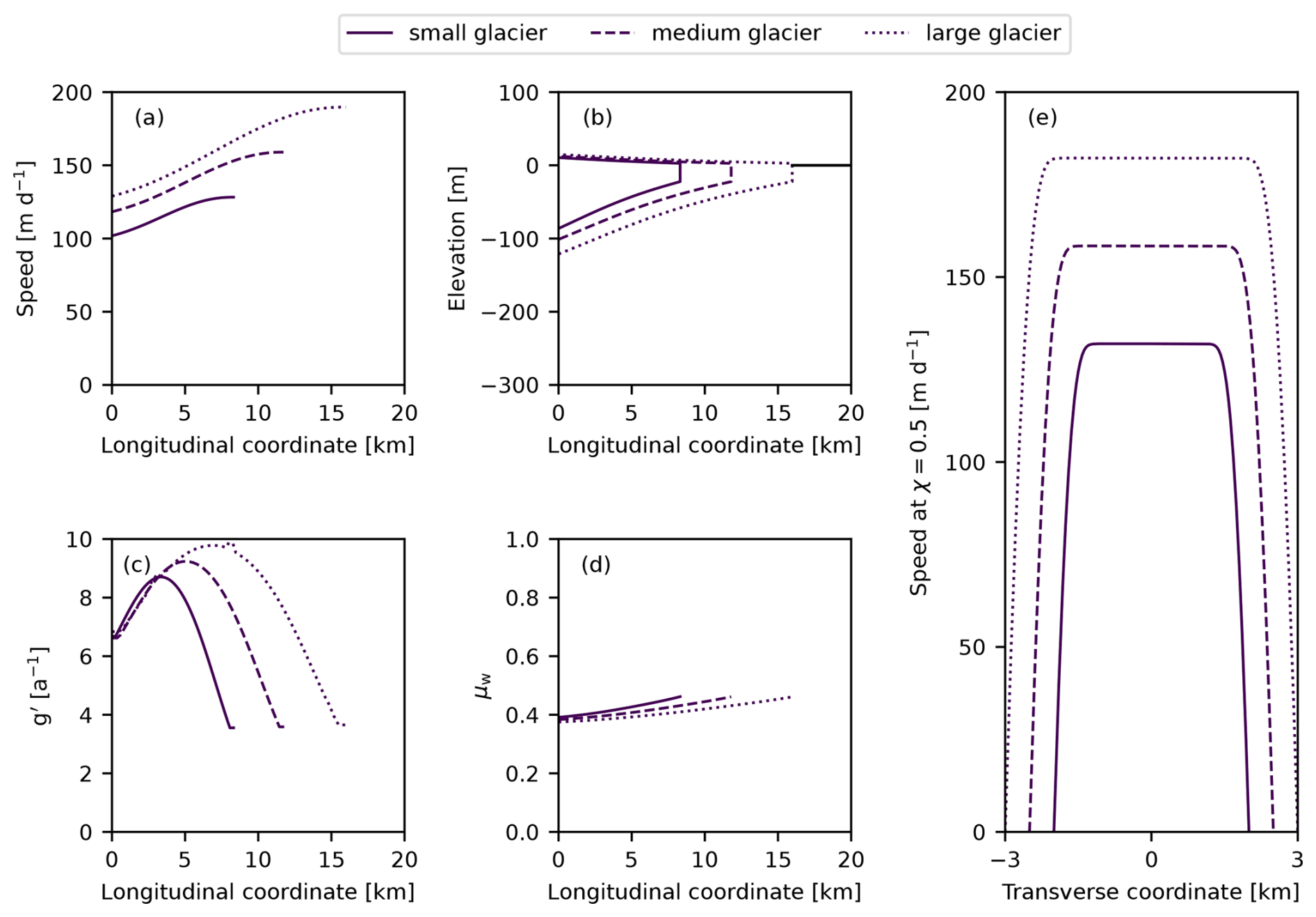
Figure 4 Steady-state profiles for variously sized glaciers as follows: (small glacier: solid lines) $U_{\mathrm{t}}=U_{\mathrm{c}}=\mathrm{6000}$ m a⁻¹, H_t=600 m, and W=4000 m; (medium glacier: dashed lines) $U_{\mathrm{t}}=U_{\mathrm{c}}=\mathrm{7000}$ m a⁻¹, H_t=700 m, and W=5000 m; (large glacier: dotted lines) $U_{\mathrm{t}}=U_{\mathrm{c}}=\mathrm{8000}$ m a⁻¹, H_t=800 m, and W=6000 m. (a–d) Longitudinal profiles of velocity, thickness, granular fluidity, and limit of internal friction along the fjord walls. (e) Transverse velocity profiles at the ice mélange midpoint. For all simulations, $\dot{B}=-\mathrm{0.8}$ m d⁻¹, d=25 m, μ_s=0.3, A=0.5, and $b=\mathrm{1}\times {\mathrm{10}}^{\mathrm{4}}$. Longitudinal coordinates are relative to the glacier terminus.

We next considered the impact of surface and basal melting on ice mélange characteristics. Iceberg melt rates in fjords can range from 0.1–0.8 m d⁻¹ (Enderlin et al., 2016), and icebergs are particularly important sources of freshwater in winter (Moon et al., 2017). We find that ice mélange thickness and length are sensitive to melt (Fig. 5a) due to the effect of melt on lateral shear stresses and that the buttressing force depends on the melt rate through an inverse power-law relationship with an exponent of about −3 (Fig. 5b).

Finally, fjord width also has important impacts on the ice mélange extent and buttressing force. Increasing the fjord width reduces the ability of shear stresses to build an ice mélange wedge, and thus the ice mélange is thinner and sheds icebergs more readily. Consequently the buttressing force decays roughly exponentially with fjord width (Fig. 6a–b), as also observed in the analysis of quasi-static flow (Amundson and Burton, 2018; Burton et al., 2018). The width gradient has similar effects on the buttressing force. Converging walls ($\mathrm{d}W/\mathrm{d}x<\mathrm{0}$) create extra flow resistance that allows for the development of a thicker ice mélange wedge. The buttressing force also decays roughly exponentially with the width gradient (Fig. 6c–d).

Figure 5 Effect of melt rates on (a) steady-state thickness profiles and (b) the ice mélange buttressing force per unit width. The dotted curve represents force estimates computed by neglecting longitudinal strain rates, whereas the dashed curve includes the effect of longitudinal strain rates. For all simulations, $U_{\mathrm{t}}=U_{\mathrm{c}}=\mathrm{6000}$ m a⁻¹, H_t=600 m, W=4000 m, d=25 m, μ_s=0.3, A=0.5, and $b=\mathrm{1}\times {\mathrm{10}}^{\mathrm{4}}$.

Figure 6 Effect of fjord geometry on steady-state thickness profiles and the buttressing force per unit width. In (a) and (b) the width was varied while the gradient in width was held constant. In (c) and (d) the width at the glacier terminus was fixed at 4000 m and the gradient in width was varied. Positive (negative) values of $\mathrm{d}W/\mathrm{d}x$ correspond to fjord walls that are diverging (converging). The dotted curves represent force estimates computed by neglecting longitudinal strain rates, whereas the dashed curves includes the effect of longitudinal strain rates. For all simulations, $U_{\mathrm{t}}=U_{\mathrm{c}}=\mathrm{6000}$ m a⁻¹, H_t=600 m, d=25 m, μ_s=0.3, A=0.5, and $b=\mathrm{1}\times {\mathrm{10}}^{\mathrm{4}}$.

3.2 Transient simulations

The ice mélange buttressing force is clearly sensitive to changes in ice mélange thickness. From field and remote sensing observations, we expect ice mélange to be weakest in summer, when melt rates and calving activity are highest (e.g., Joughin et al., 2020). To investigate the implications of these fluctuations, we impose seasonal variations in melting and calving rates with amplitudes of 0.2 m d⁻¹ and 600 m a⁻¹, respectively.

We find that the buttressing force decreases as the melt rate increases (Fig. 7a–b), as might be expected during the summer months. However, there is a lag of 2 months between the highest melt rates and the weakest ice mélange. The lag is smallest for ice mélange experiencing higher melt rates because smaller ice mélange will respond more rapidly to external forcings. There is also less variability in the buttressing force for smaller ice mélange.

Iceberg calving also varies seasonally and tends to be highest in the summer. The model, which assumes the ice mélange remains well packed year-round, predicts that it will thicken and grow in response to the addition of new material. As with melting, there is a lag of 2 months between variations in calving rates and the force exerted on the glacier termini, and the amplitude of the variations in force also decrease with ice mélange extent (Fig. 7c–d). Thus, melt and calving, which both vary seasonally, have opposite effects on the model behavior.

Following observations that suggest that iceberg calving is affected by the ice mélange buttressing force, we use an ad hoc linear relationship between calving and the buttressing force to begin investigating their coupled impacts on ice mélange. We suppose that

$$\begin{array}{}\text{(31)}& U_{\mathrm{c}}=\mathrm{2}{U}_{\mathrm{c},\mathrm{ss}}-{\displaystyle \frac{U_{\mathrm{c},\mathrm{ss}}}{F_{\mathrm{ss}}}}F,\end{array}$$

where U_c,ss and F_ss are the steady-state calving rate and buttressing force for a given set of model parameters. An imposed variation in melt rates causes F to vary, which is coupled to the calving rate via a negative feedback loop. This coupling reduces the lag time between the melt rate and the buttressing force to about 0.1 a, and, as a result, the calving rate is high when melt rates are also high (Fig. 7).

Figure 7 Ice mélange response to temporally varying melt rates and calving rates. (a) Sinusoidal variations in the melt rate (dashed curve) and buttressing force (solid curves). (b) Hysteresis curves between the buttressing force and melt rate for different baseline melt rates (and therefore ice mélange sizes). (c) Sinusoidal variations in the calving rates (dashed lines) and buttressing force (solid lines). (d) Hysteresis curves between the buttressing force and calving rate for different baseline melt rates (same as in panel b). The starting points of the hysteresis curves in (b) and (d) are indicated by dots. The black curves in (a) and (b) correspond to a simulation in which the calving rate depends linearly on the buttressing force. For all simulations, d=25 m, μ_s=0.3, A=0.5, and $b=\mathrm{1}\times {\mathrm{10}}^{\mathrm{4}}$.

3.3 Buttressing forces in the steady-state and quasi-static regimes

The ice mélange buttressing force depends on the thickness, tectonic stress R_xx, and granular static pressure $\stackrel{\mathrm{̃}}{P}$ at the glacier–ice mélange boundary (Eq. 30). In the quasi-static limit, the velocity gradient is zero and therefore the buttressing force scales with $H_{\mathrm{0}}^{\mathrm{2}}$. However, we find that when calving and melting are nonzero, the flow is extensional, which causes the buttressing force to be less than would be expected if buttressing force estimates were based solely on ice thickness (Figs. 5 and 6).

We find that, for parallel-sided fjords, the buttressing force in the steady-state regime also scales with $H_{\mathrm{0}}^{\mathrm{2}}$ despite the complexity introduced by nonzero strain rates (Fig. 8). During our transient simulations, the buttressing force circles around the initial steady-state solutions as the flow becomes more/less extensional. We never observe compressional flow in our simulations, and field and remote sensing observations indicate that compressional flow only occurs during and in the immediate aftermath of iceberg calving events (Peters et al., 2015; Amundson and Burton, 2018; Cassotto et al., 2021). Thus, observations of ice mélange thickness from satellite data, along with the quasi-static approximation of Eq. (30), can be used to provide an upper bound on the ice mélange buttressing force.

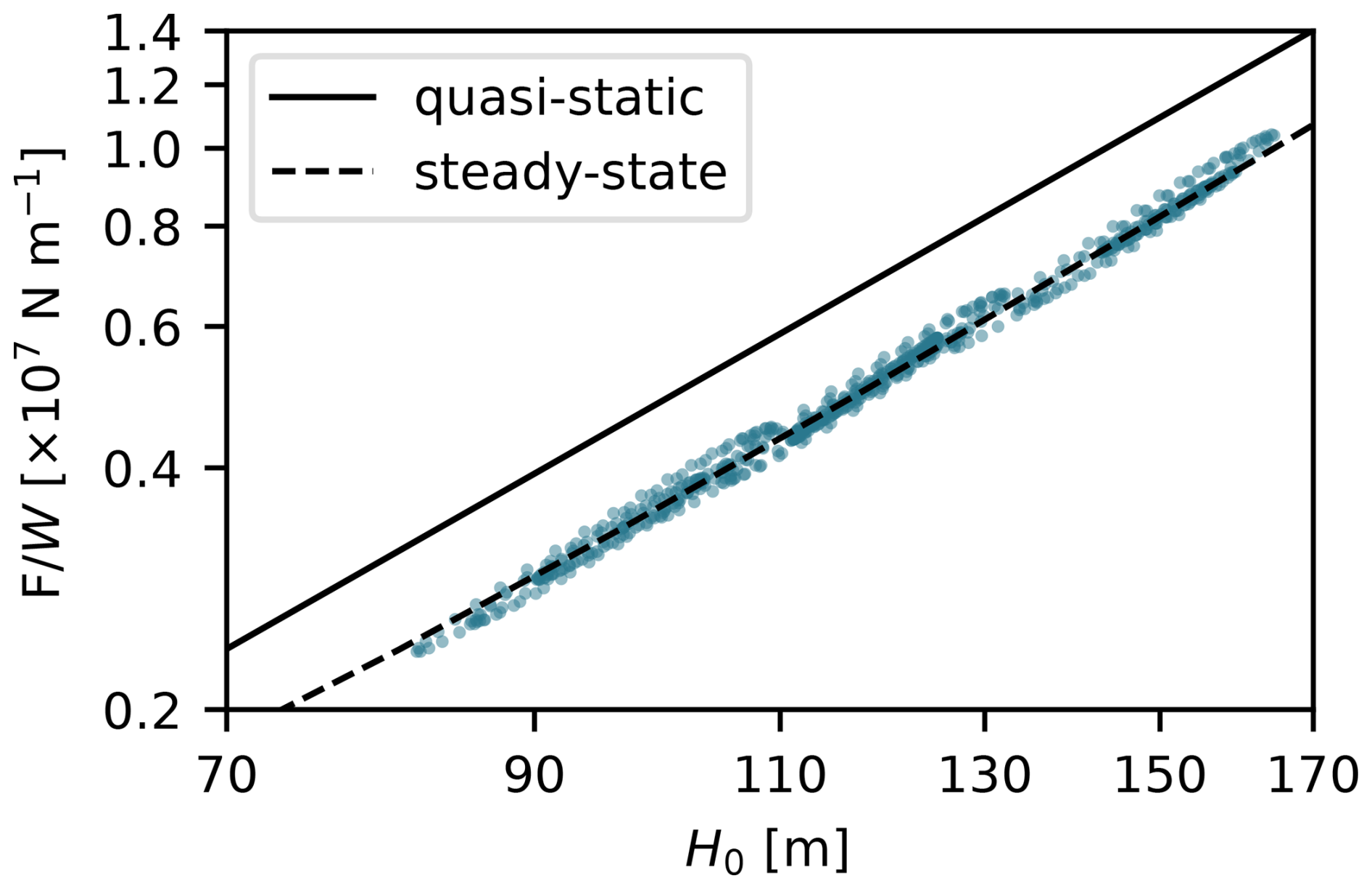
Figure 8 Relationship between the ice mélange buttressing force and thickness at x₀. The solid black line represents the quasi-static regime, the dashed black line represents the results from steady-state solutions shown in Fig. 5, and the colored dots represent the solutions for all of the transient simulations shown in Fig. 7.

4 Conclusions

We have developed a depth-averaged continuum model of ice mélange flow, which we refer to as the nonlocal shallow mélange approximation, that is based on recent advances in our understanding of granular materials and that is suitable for long-timescale glacier simulations. Consistent with other granular flows, the model exhibits viscous flow where the stresses are far from the yield point and plug flow where the stresses approach the yield point.

The model contains four parameters (the iceberg size, two dimensionless constants, and the static yield coefficient) that must be tuned. We have selected a set of parameters that produce velocity and thickness profiles that are roughly consistent with remote sensing observations from Greenland (Foga et al., 2014; Amundson and Burton, 2018; Bevan et al., 2019; Xie et al., 2019). Ultimately, the profiles depend on the ice mélange stiffness; stiff ice mélange does not spread very easily and tends to result in thick, extensive ice coverage. Each of the four model parameters can affect the overall fluidity; thus, other parameter combinations may also produce suitable model results. Determining the best parameter values that work across a range of forcing and fjord geometries remains a major task for laboratory experiments and field observations.

We assume that the ice mélange is well packed and homogeneous, and we do not account for cohesion. The model is likely to perform best for winter ice mélange and for systems where ice mélange persists year-round since the flow approximation is not applicable for granular materials far from the well-packed limit. The impacts of iceberg heterogeneity and cohesion on ice mélange flow require further investigation. We suggest that both could potentially be incorporated into our modeling framework through modification of the model parameters, which are currently treated as constants, and/or by tuning the model parameters with field observations, laboratory experiments, and discrete element simulations. Future work should also attempt to quantify the degree to which the quasi-one-dimensional model can replicate the behavior of ice mélange in fjords with complex geometry.

Ultimately, we find that the nonlocal shallow mélange approximation produces thickness and velocity profiles that are roughly consistent with previously published field observations (Amundson and Burton, 2018; Bevan et al., 2019; Xie et al., 2019) and evolves in response to glaciological, atmospheric, and oceanographic forcing. Ice fluxes, melt rates, and fjord geometry strongly affect the model geometry and ice mélange buttressing forces. Addition of new material into the ice mélange via iceberg calving makes it longer, thicker, and more resistive, whereas removal of material through surface and basal melting does the opposite. Thus the model may be capable of explaining temporal variations in buttressing forces and why ice mélange appears to have larger impacts in some glacier–fjord systems than it does in others.

Appendix A: Coordinate stretching

We use a coordinate system that moves with the glacier terminus, and, following Schoof (2007), we introduce coordinate stretching to deal with the moving boundary at the end of the ice mélange (x=L),

$$\begin{array}{}\text{(A1)}& \mathit{\chi }={\displaystyle \frac{x}{L}},\end{array}$$

which maps $\mathrm{0}\le x\le L$ to $\mathrm{0}\le \mathit{\chi }\le \mathrm{1}$. According to the chain rule,

$$\begin{array}{}\text{(A2)}& {\displaystyle \frac{\partial }{\partial x}}={\displaystyle \frac{\partial \mathit{\chi }}{\partial x}}{\displaystyle \frac{\partial }{\partial \mathit{\chi }}}={\displaystyle \frac{\mathrm{1}}{L}}{\displaystyle \frac{\partial }{\partial \mathit{\chi }}}.\end{array}$$

The coordinate stretching also necessitates a transformation of time derivatives. The material derivative is

$$\begin{array}{}\text{(A3)}& {\displaystyle \frac{\mathrm{D}}{\mathrm{D}t}}={\displaystyle \frac{\mathrm{d}x}{\mathrm{d}t}}{\displaystyle \frac{\partial }{\partial x}}+{\displaystyle \frac{\partial }{\partial t}}.\end{array}$$

The grid points move with velocity:

$$\begin{array}{}\text{(A4)}& {\displaystyle \frac{\mathrm{d}x}{\mathrm{d}t}}=\mathit{\chi }{\displaystyle \frac{\mathrm{d}L}{\mathrm{d}t}}.\end{array}$$

The material derivative of a quantity that is moving with the grid is the same as the partial derivative of that same quantity in the grid's reference frame. As in Schoof (2007), we therefore let t=τ to distinguish between partial derivatives when x and χ are held constant, respectively, which allows us to replace $D/Dt$ with $\partial /\partial \mathit{\tau }$. Thus, after rearranging Eq. (A3) and inserting Eqs. (A2) and (A4), we arrive at

$$\begin{array}{}\text{(A5)}& {\displaystyle \frac{\partial }{\partial t}}={\displaystyle \frac{\partial }{\partial \mathit{\tau }}}-{\displaystyle \frac{\mathit{\chi }}{L}}{\displaystyle \frac{\mathrm{d}L}{\mathrm{d}\mathit{\tau }}}{\displaystyle \frac{\partial }{\partial \mathit{\chi }}}.\end{array}$$

The coordinate transformations are then applied to the stress balance, granular fluidity, and mass continuity equations (Eqs. 21, 16, and 27), yielding

$$\begin{array}{}\text{(A6)}& \begin{array}{rl}& {\displaystyle \frac{\mathrm{1}}{L}}{\displaystyle \frac{\partial }{\partial \mathit{\chi }}}\left({\displaystyle \frac{\mathrm{1}}{g^x+(\partial U/\partial \mathit{\chi })/L}}{H}^{\mathrm{2}}{\displaystyle \frac{\mathrm{1}}{L}}{\displaystyle \frac{\partial U}{\partial \mathit{\chi }}}\right)={\displaystyle \frac{H}{L}}{\displaystyle \frac{\partial H}{\partial \mathit{\chi }}}\\ & +{\displaystyle \frac{H^{\mathrm{2}}}{W}}{\mathit{\mu }}_{\mathrm{w}}\mathrm{sgn}\left(U\right)\\ & {\displaystyle \frac{\mathrm{1}}{L^{\mathrm{2}}}}{\displaystyle \frac{{\partial }^{\mathrm{2}}{g}^x}{\partial {\mathit{\chi }}^{\mathrm{2}}}}={\displaystyle \frac{\mathrm{1}}{{\mathit{\xi }}^{\mathrm{2}}}}\left(g^x-g_{\mathrm{loc}}^x\right)\\ & {\displaystyle \frac{\partial H}{\partial \mathit{\tau }}}-{\displaystyle \frac{\mathit{\chi }}{L}}{\displaystyle \frac{\mathrm{d}L}{\mathrm{d}\mathit{\tau }}}{\displaystyle \frac{\partial H}{\partial \mathit{\chi }}}+{\displaystyle \frac{\mathrm{1}}{WL}}{\displaystyle \frac{\partial }{\partial \mathit{\chi }}}\left(UHW\right)=\dot{B}.\end{array}\end{array}$$

The granular fluidity depends on ${\dot{\mathit{ϵ}}}_e$, which is transformed as

$$\begin{array}{}\text{(A7)}& {\dot{\mathit{ϵ}}}_e={\displaystyle \frac{{\dot{\mathit{ϵ}}}_{\mathit{\chi }}}{L}},\end{array}$$

where ${\dot{\mathit{ϵ}}}_{\mathit{\chi }}$ is the second invariant of the strain rate in the stretched coordinate system. The transverse velocity equation is unaffected by the coordinate transformation.

Appendix B: Nondimensionalization

We nondimensionalize the model equations to improve model convergence. We start by assuming that we know characteristic scales for the length [L], velocity [U], and mass balance rate $\left[\dot{B}\right]$. We then set scales for the thickness and time:

$$\begin{array}{}\text{(B1)}& \begin{array}{rl}& \left[L\right]={\displaystyle \frac{\left[U\right]\left[H\right]}{\left[\dot{B}\right]}}\\ & \left[\mathit{\tau }\right]={\displaystyle \frac{\left[L\right]}{\left[U\right]}}.\end{array}\end{array}$$

The model is scaled by defining

$$\begin{array}{}\text{(B2)}& \begin{array}{rl}& L=\left[L\right]L^{*}\\ & H=\left[H\right]H^{*}\\ & U=\left[U\right]U^{*}\\ & \dot{B}=\left[\dot{B}\right]{\dot{B}}^{*}\\ & W=\left[L\right]W^{*}\\ & d=\left[H\right]d^{*},\end{array}\end{array}$$

where ^* is used to indicate dimensionless variables. We also note that $g^{\prime }=g^{\prime *}\left[U\right]/\left[L\right]$ since $g^{\prime }={\dot{\mathit{ϵ}}}_e/\mathit{\mu }$. Dropping the asterisks and defining $\mathit{\gamma }=[H{]}^{\mathrm{2}}/[L{]}^{\mathrm{2}}$, the nondimensional stress balance, granular fluidity, transverse velocity, and mass continuity equations become

$$\begin{array}{}\text{(B3)}& \begin{array}{rl}& {\displaystyle \frac{\mathrm{1}}{L^{\mathrm{2}}}}{\displaystyle \frac{\partial }{\partial \mathit{\chi }}}\left({\displaystyle \frac{H^{\mathrm{2}}}{g^x+(\partial U/\partial x)/L}}{\displaystyle \frac{\partial U}{\partial \mathit{\chi }}}\right)={\displaystyle \frac{H}{L}}{\displaystyle \frac{\partial H}{\partial \mathit{\chi }}}\\ & +{\displaystyle \frac{H^{\mathrm{2}}}{W}}{\mathit{\mu }}_{\mathrm{w}}\mathrm{sgn}\left(U\right)\\ & {\displaystyle \frac{\mathit{\gamma }}{L^{\mathrm{2}}}}{\displaystyle \frac{{\partial }^{\mathrm{2}}{g}^x}{\partial {\mathit{\chi }}^{\mathrm{2}}}}={\displaystyle \frac{\mathrm{1}}{{\mathit{\xi }}^{\mathrm{2}}}}\left(g^x-g_{\mathrm{loc}}^x\right)\\ & \mathit{\gamma }{\displaystyle \frac{{\partial }^{\mathrm{2}}{g}^y}{\partial y^{\mathrm{2}}}}={\displaystyle \frac{\mathrm{1}}{{\mathit{\xi }}^{\mathrm{2}}}}\left(g^y-g_{\mathrm{loc}}^y\right)\\ & U+(U_{\mathrm{t}}-U_{\mathrm{c}})={\displaystyle \frac{\mathrm{2}}{W}}\underset{\mathrm{0}}{\overset{W/\mathrm{2}}{\int }}\underset{\mathrm{0}}{\overset{y}{\int }}\mathrm{2}{\mathit{\mu }}_{\mathrm{w}}\left(\mathrm{1}-{\displaystyle \frac{\mathrm{2}y}{W}}\right)g^y\mathrm{d}{y}^{\prime }\mathrm{d}y\\ & {\displaystyle \frac{\partial H}{\partial \mathit{\tau }}}-{\displaystyle \frac{\mathit{\chi }}{L}}{\displaystyle \frac{\mathrm{d}L}{\mathrm{d}\mathit{\tau }}}{\displaystyle \frac{\partial H}{\partial \mathit{\chi }}}+{\displaystyle \frac{\mathrm{1}}{WL}}{\displaystyle \frac{\partial }{\partial \mathit{\chi }}}\left(UHW\right)=\dot{B}.\end{array}\end{array}$$

Using dimensionless variables, the cooperativity length and local granular fluidity are calculated as

$$\begin{array}{}\text{(B4)}& \mathit{\xi }={\displaystyle \frac{Ad}{\sqrt{|\mathit{\mu }-{\mathit{\mu }}_{\mathrm{s}}|}}}\end{array}$$

and

$$\begin{array}{}\text{(B5)}& g_{\mathrm{loc}}^x=g_{\mathrm{loc}}^y=\left\{\begin{array}{ll}\frac{\left[L\right]}{\left[U\right]}\sqrt{\frac{P}{\mathit{\rho }{d}^{\mathrm{2}}\left[H\right]}}\frac{(\mathit{\mu }-{\mathit{\mu }}_{\mathrm{s}})}{\mathit{\mu }b}& \text{if}\mathit{\mu }>{\mathit{\mu }}_{\mathrm{s}}\\ \mathrm{0}& \text{if}\mathit{\mu }\le {\mathit{\mu }}_{\mathrm{s}}.\end{array}\right.\end{array}$$

When calculating g^x, the effective coefficient of friction is given by $\mathit{\mu }=({\dot{\mathit{ϵ}}}_{\mathit{\chi }}/L+\mathit{\delta }\dot{\mathit{ϵ}})/g^x$, and when calculating g^y, it is given by $\mathit{\mu }={\mathit{\mu }}_{\mathrm{w}}(\mathrm{1}-\mathrm{2}y/W)$ and $\partial u/\partial y=\mathrm{2}\mathit{\mu }{g}^y$.

The boundary conditions are unchanged in dimensionless variables.

Appendix C: Finite-difference discretization

We use finite differences with a staggered grid and implicit time step to simultaneously calculate U, g^x, μ_w, H, and L at each time step. Indices j and n refer to grid points and time steps. We define $j=\mathrm{0}:N$ so that there are N+1 grid points each for U and μ_w and N points each for H and g^x. Altogether the model solves for 4N+3 unknowns in the x direction. The discretized stress balance, granular fluidity, μ_w, and mass continuity equations provide 4N+2 equations. One additional equation comes from defining the end of the ice mélange as being where the thickness equals the grain size:

$$\begin{array}{}\text{(C1)}& \mathrm{3}{H}_{N-\mathrm{1}/\mathrm{2}}-H_{N-\mathrm{3}/\mathrm{2}}=d.\end{array}$$

C1 Stress balance equation

The discretized stress balance equation is

$$\begin{array}{}\text{(C2)}& \begin{array}{rl}{\displaystyle \frac{\mathrm{1}}{(L\mathrm{\Delta }\mathit{\chi }{)}^{\mathrm{2}}}}& \left[{\mathit{\nu }}_{j-\mathrm{1}/\mathrm{2}}{U}_{j-\mathrm{1}}-\left({\mathit{\nu }}_{j+\mathrm{1}/\mathrm{2}}+{\mathit{\nu }}_{j-\mathrm{1}/\mathrm{2}}\right)U_j+{\mathit{\nu }}_{j+\mathrm{1}/\mathrm{2}}{U}_{j+\mathrm{1}}\right]\\ & ={\displaystyle \frac{\mathrm{1}}{L\mathrm{\Delta }\mathit{\chi }}}{\displaystyle \frac{H_{j+\mathrm{1}/\mathrm{2}}+H_{j-\mathrm{1}/\mathrm{2}}}{\mathrm{2}}}\left(H_{j+\mathrm{1}/\mathrm{2}}-H_{j-\mathrm{1}/\mathrm{2}}\right)\\ & +{\displaystyle \frac{\mathrm{1}}{\mathrm{2}}}{\displaystyle \frac{{\left(H_{j+\mathrm{1}/\mathrm{2}}+H_{j-\mathrm{1}/\mathrm{2}}\right)}^{\mathrm{2}}}{W_{j+\mathrm{1}/\mathrm{2}}+W_{j-\mathrm{1}/\mathrm{2}}}}{\mathit{\mu }}_{w,j}\mathrm{sgn}\left(U_j\right),\end{array}\end{array}$$

which is used for $j=\mathrm{1}:N-\mathrm{1}$ and where we have defined

$$\begin{array}{}\text{(C3)}& {\mathit{\nu }}_{j-\mathrm{1}/\mathrm{2}}={\displaystyle \frac{H_{j-\mathrm{1}/\mathrm{2}}^{\mathrm{2}}}{g_{j-\mathrm{1}/\mathrm{2}}^x+(U_j-U_{j-\mathrm{1}})/\left(L\mathrm{\Delta }\mathit{\chi }\right)}}.\end{array}$$

The upstream boundary condition is $U_{\mathrm{0}}=U_c{H}_{\mathrm{t}}/H_{\mathrm{0}}$ (Eq. 22), while the downstream boundary condition is $U_N-U_{N-\mathrm{1}}=\mathrm{0}$ (Eq. 23).

C2 Nonlocal granular fluidity equation

The equation for the granular fluidity is discretized using a standard difference formula such that

$$\begin{array}{}\text{(C4)}& \begin{array}{rl}\mathit{\gamma }& {\displaystyle \frac{g_{j-\mathrm{3}/\mathrm{2}}^x-\mathrm{2}{g}_{j-\mathrm{1}/\mathrm{2}}^x+g_{j+\mathrm{1}/\mathrm{2}}^x}{(L\mathrm{\Delta }\mathit{\chi }{)}^{\mathrm{2}}}}\\ & ={\displaystyle \frac{\mathrm{1}}{{\mathit{\xi }}_{j-\mathrm{1}/\mathrm{2}}^{\mathrm{2}}}}\left(g_{j-\mathrm{1}/\mathrm{2}}^x-g_{\mathrm{loc},j-\mathrm{1}/\mathrm{2}}^x\right),\end{array}\end{array}$$

with boundary conditions $g_{\mathrm{3}/\mathrm{2}}^x-g_{\mathrm{1}/\mathrm{2}}^x=\mathrm{0}$ and $g_{N-\mathrm{1}/\mathrm{2}}^x-g_{N-\mathrm{3}/\mathrm{2}}^x=\mathrm{0}$ ($\partial g^x/\partial x=\mathrm{0}$ at $x=\mathrm{0},L$). The granular fluidity is only calculated on N grid points because it depends on the velocity gradient, which we calculate using a one-sided difference. As result, $g_{j-\mathrm{1}/\mathrm{2}}^x$ depends on U_j and U_j−1. Similarly, $g_{\mathrm{loc},j-\mathrm{1}/\mathrm{2}}^x$ (Eq. 17) depends on U_j and U_j−1 as well as $H_{j-\mathrm{1}/\mathrm{2}}$.

C3 Transverse velocity equation

We calculate transverse velocity profiles at each χ grid point. We use M+1 grid points in the y direction. The discretized granular fluidity equation in the y direction is then

$$\begin{array}{}\text{(C5)}& \mathit{\gamma }{\displaystyle \frac{g_{m-\mathrm{1}}^y-\mathrm{2}{g}_m^y+g_{m+\mathrm{1}}^y}{\mathrm{\Delta }{y}^{\mathrm{2}}}}={\displaystyle \frac{\mathrm{1}}{{\mathit{\xi }}_m^{\mathrm{2}}}}\left(g_m^y-g_{\mathrm{loc},m}^y\right).\end{array}$$

At the boundaries we set $\mathrm{d}{g}^y/\mathrm{d}y=\mathrm{0}$, and therefore $g_{\mathrm{1}}^y-g_{\mathrm{0}}^y=\mathrm{0}$ and $g_M^y-g_{M-\mathrm{1}}^y=\mathrm{0}$. $g_{\mathrm{loc},m}^y$ and ξ_m both depend on μ (see Eqs. 17 and 18). For shear-dominated flow, μ varies linearly across the fjord (Eq. 24). Therefore, for a given value of μ_w, $g_{\mathrm{loc},m}^y$ and ξ_m can be directly calculated. Equation (C5) is then solved to determine g^y(y).

Finally, we integrate Eq. (25) twice to find the average velocity in the transect, which is required to equal the velocity U in the ice mélange's reference frame plus the glacier terminus velocity:

$$\begin{array}{}\text{(C6)}& U_j+U_{\mathrm{t}}-U_{\mathrm{c}}={\displaystyle \frac{\mathrm{2}}{W_j}}\underset{\mathrm{0}}{\overset{W_j/\mathrm{2}}{\int }}\underset{\mathrm{0}}{\overset{y}{\int }}{\mathit{\mu }}_{w,j}\left(\mathrm{1}-{\displaystyle \frac{\mathrm{2}{y}^{\prime }}{W_j}}\right)g^y\mathrm{d}{y}^{\prime }\mathrm{d}y.\end{array}$$

C4 Mass continuity equation

For the mass continuity equation, we use an upwind scheme with a backward Euler step; the advective term is discretized with centered differences:

$$\begin{array}{}\text{(C7)}& \begin{array}{rl}& {\displaystyle \frac{H_{j+\mathrm{1}/\mathrm{2}}-H_{j+\mathrm{1}/\mathrm{2}}^{\star }}{\mathrm{\Delta }\mathit{\tau }}}-\left({\mathit{\chi }}_{j+\mathrm{1}/\mathrm{2}}{\displaystyle \frac{\mathrm{d}L}{\mathrm{d}\mathit{\tau }}}\right){\displaystyle \frac{H_{j+\mathrm{3}/\mathrm{2}}-H_{j-\mathrm{1}/\mathrm{2}}}{\mathrm{2}L\mathrm{\Delta }\mathit{\chi }}}\\ & +{\displaystyle \frac{\left(U_{j+\mathrm{1}}+U_j\right)H_{j+\mathrm{1}/\mathrm{2}}{W}_{j+\mathrm{1}/\mathrm{2}}-\left(U_j+U_{j-\mathrm{1}}\right)H_{j-\mathrm{1}/\mathrm{2}}{W}_{j-\mathrm{1}/\mathrm{2}}}{\mathrm{2}{W}_{j+\mathrm{1}/\mathrm{2}}L\mathrm{\Delta }\mathit{\chi }}}\\ & ={\dot{B}}_{j+\mathrm{1}/\mathrm{2}},\end{array}\end{array}$$

where superscript ^⋆ is now used to refer to values from the previous time step. At both boundaries (j=0 and $j=N-\mathrm{1}$) we use one-sided differences for the advective term, and at the upstream boundary (j=0) we use a forward difference for the diffusive term. Consequently, the discretized mass continuity equations at the upstream and downstream boundaries are

$$\begin{array}{}\text{(C8)}& \begin{array}{rl}{\displaystyle \frac{H_{\mathrm{1}/\mathrm{2}}-H_{\mathrm{1}/\mathrm{2}}^{\star }}{\mathrm{\Delta }\mathit{\tau }}}& -\left({\mathit{\chi }}_{\mathrm{1}/\mathrm{2}}{\displaystyle \frac{\mathrm{d}L}{\mathrm{d}\mathit{\tau }}}\right){\displaystyle \frac{H_{\mathrm{3}/\mathrm{2}}-H_{\mathrm{1}/\mathrm{2}}}{L\mathrm{\Delta }\mathit{\chi }}}\\ & +{\displaystyle \frac{\left(U_{\mathrm{2}}+U_{\mathrm{1}}\right)H_{\mathrm{3}/\mathrm{2}}{W}_{\mathrm{3}/\mathrm{2}}-\left(U_{\mathrm{1}}+U_{\mathrm{0}}\right)H_{\mathrm{1}/\mathrm{2}}{W}_{\mathrm{1}/\mathrm{2}}}{\mathrm{2}{W}_{\mathrm{1}/\mathrm{2}}L\mathrm{\Delta }\mathit{\chi }}}\\ & ={\dot{B}}_{\mathrm{1}/\mathrm{2}}\end{array}\end{array}$$

and

$$\begin{array}{}\text{(C9)}& \begin{array}{rl}& {\displaystyle \frac{H_{N-\mathrm{1}/\mathrm{2}}-H_{N-\mathrm{1}/\mathrm{2}}^{\star }}{\mathrm{\Delta }\mathit{\tau }}}-\left({\mathit{\chi }}_{N-\mathrm{1}/\mathrm{2}}{\displaystyle \frac{\mathrm{d}L}{\mathrm{d}\mathit{\tau }}}\right){\displaystyle \frac{H_{N-\mathrm{1}/\mathrm{2}}-H_{N-\mathrm{3}/\mathrm{2}}}{L\mathrm{\Delta }\mathit{\chi }}}\\ & +{\displaystyle \frac{\left(U_N+U_{N-\mathrm{1}}\right)H_{N-\mathrm{1}/\mathrm{2}}{W}_{N-\mathrm{1}/\mathrm{2}}-\left(U_{N-\mathrm{1}}+U_{N-\mathrm{2}}\right)H_{N-\mathrm{3}/\mathrm{2}}{W}_{N-\mathrm{3}/\mathrm{2}}}{\mathrm{2}{W}_{N-\mathrm{1}/\mathrm{2}}L\mathrm{\Delta }\mathit{\chi }}}\\ & ={\dot{B}}_{N-\mathrm{1}/\mathrm{2}}.\end{array}\end{array}$$

Appendix D: Description of model variables

Variable	Description
ρ, ρw	densities of ice and water
$\mathit{x}=\langle x,y,z\rangle$	position vector
g, geff, t	gravitational acceleration, effective gravity, and time
$\mathit{u}=\langle u,v,w\rangle$	velocity vector
${\dot{\mathit{ϵ}}}_{ij}$, ${\dot{\mathit{ϵ}}}_e$	strain rate tensor and effective strain rate
σij, ${\mathit{\sigma }}_{ij}^{\prime }$, Rij	stress, deviatoric stress, and tectonic stress tensors
δij	Kronecker delta
$\stackrel{\mathrm{̃}}{p}$	granular static pressure
P, $\stackrel{\mathrm{̃}}{P}$	depth-averaged pressure and granular static pressure
W, L, U, H	width, length, and depth- and width-averaged velocity and thickness
Ht, Ut, Uc	depth- and width-averaged (glacier) terminus thickness, terminus velocity, and calving rate
H0, U0	thickness and depth- and width-averaged velocity at x=0
F	buttressing force
$\dot{B}$	surface plus basal mass balance rate
μ, μw	effective coefficient of friction within the ice mélange and along the fjord walls
μs	static yield coefficient
g′, $g_{\mathrm{loc}}^{\prime }$	granular fluidity and local granular fluidity
gx, gy	granular fluidity for extension-dominated and shear-dominated flow
ξ	cooperativity length
d	characteristic iceberg diameter
b, A	dimensionless parameters
$\mathit{\delta }\dot{\mathit{ϵ}}$	finite strain rate parameter
χ, τ, ${\dot{\mathit{ϵ}}}_{\mathit{\chi }}$	longitudinal position, time, and effective strain rate in the stretched coordinate system