Multiple modes of shoreline change along the Alaskan Beaufort Sea observed using ICESat-2 altimetry and satellite imagery

Arctic shorelines are retreating rapidly due to declining sea ice cover, increasing temperatures, and increasing storm activity. Shoreline morphology may influence local retreat rates, but quantifying this relationship requires repeat estimates of shoreline positions and morphologic properties. Here we use a novel combination of shoreline boundaries from multispectral imagery from Planet and topographic profiles from the Ice, Cloud and land Elevation Satellite 2 (ICESat-2) altimeter to compare year-to-year changes in shoreline position and morphology across different shoreline types, focusing on an 8 km stretch of the Alaskan Beaufort Sea coast during the 2019–2021 open-water seasons. We consider temporal and spatial variability in shoreline change in the context of environmental forcings from ERA5 and morphologic classifications from the ShoreZone database. We find a mean spatially averaged shoreline change rate of −16.5 m a⁻¹ over 3 years, with local estimates ranging from −66.7 to +18.6 m in a single year. We posit that annual and kilometer-scale variability in shoreline change can be explained by the response of different geomorphic units to time-varying wave and ocean conditions. Ice-rich coastal bluffs and inundated tundra exhibited high retreat that is likely driven by high temperatures and wave exposure, while the stretch of shoreline with vegetated peat in front of a large breached thermokarst lake remained relatively stable. Our topographic profiles from ICESat-2 sample three distinct shoreline types (a bluff, a small drained lake basin, and a dune in front of a large drained lake basin) that exhibit different patterns of shoreline change (in terms of both position and morphology) over the 3-year study period. Analysis of altimetry-derived morphologic parameters such as elevation and slope and small-scale features such as toppled blocks and surface ponding provide insight into specific erosion and accretion processes that drive shoreline change. We conclude that repeat altimetry measurements from ICESat-2 and multispectral imagery provide complementary observations that illustrate how both the position and the topography of the shoreline are changing in response to a changing Arctic.

1 Introduction

Decreasing sea ice extent (Overeem et al., 2011; Baranskaya et al., 2021), increasing air (Serreze and Barry, 2011; Baranskaya et al., 2021) and ocean (Timmermans and Labe, 2023) temperatures, and increasing storm frequency (Manson and Solomon, 2007; Erikson et al., 2020; Baranskaya et al., 2021) are driving widespread erosion across Arctic coasts. Pan-Arctic shoreline change rates over the second half of the 20th century have been estimated to be −0.5 m a⁻¹ (where negative shoreline change indicates retreat), with the Alaskan Beaufort Sea coast changing at an elevated rate of −1.5 m a⁻¹ (Lantuit et al., 2012). This erosion threatens coastal communities through damage to infrastructure and cultural sites, loss of economic opportunity, and loss of access to traditional navigation routes and subsistence practices (e.g., Brady and Leichenko, 2020; Irrgang et al., 2022). Coastal erosion also adds carbon and nitrogen to the ocean, impacting primary production (e.g., Terhaar et al., 2021) and the global carbon cycle (e.g., Irrgang et al., 2022). Accurate forecasts of coastal retreat rates are needed to inform carbon cycling models and coastal resilience efforts.

During the open-water season, i.e., when the coasts are not sheltered by sea ice, the shoreline is subjected to warm ocean temperatures and mechanical energy from waves, driving ground ice thaw and erosion through thermal abrasion (Aré, 1988; Wobus et al., 2011; Günther et al., 2013; Baranskaya et al., 2021). Warm air temperatures can drive top-down ground thawing and erosion through thermal denudation (Günther et al., 2013; Baranskaya et al., 2021). Although observational studies (Nielsen et al., 2020) and models (e.g., Nielsen et al., 2022; Rolph et al., 2022) have demonstrated a correspondence between environmental drivers and decadal-scale retreat over regional scales (∼ hundreds of kilometers), studies that consider the spatial distribution of decadal and annual retreat rates have found them to be highly variable on local scales (∼ tens of meters) (Gibbs and Richmond, 2015; Farquharson et al., 2018; Irrgang et al., 2018; Jones et al., 2018; Baranskaya et al., 2021). These findings suggest that the local response of shorelines to environmental forcings is not uniform and may depend on local shoreline characteristics.

Previous work has suggested that shoreline morphology plays a role in controlling local retreat rates. Farquharson et al. (2018) found varying shoreline change patterns across different geomorphic units in the Chukchi Sea, with permafrost bluffs and barrier islands primarily retreating and beaches and gravel barriers showing a mixture of retreat and advance. Piliouras et al. (2023) found that shoreline change along the Alaskan Beaufort Sea coast varied according to elevation, lithology, and barrier island presence. Some observed differences are likely due to the fact that different geomorphic units are subject to a variety of erosive and accretive processes driven by time-varying ocean and atmospheric conditions. Steep coastal bluffs are predominately subjected to erosion from thermal abrasion at their base and thermal denudation above the water line (Wobus et al., 2011; Aré, 1988; Günther et al., 2013; Baranskaya et al., 2021; Irrgang et al., 2022). High rates of thermal abrasion can lead to bluff collapse events, where a cohesive block detaches from the shoreline. These blocks can temporarily shelter the shoreline from additional wave activity but tend to disintegrate over the span of several days (Overeem et al., 2011; Wobus et al., 2011; Barnhart et al., 2014) or weeks (Jones et al., 2018). Coastal beaches and dunes, on the other hand, are subject to erosion or accretion depending on alongshore sediment transport patterns. Observations of erosion rates and simulated wave runup models in both temperate (Earlie et al., 2018) and Arctic (Rolph et al., 2022) environments have suggested that wave-driven retreat is sensitive to shoreline geometric attributes such as beach slope and the elevation of the beach–cliff junction. Over time, erosion, accretion, and ground thaw can drive changes in shoreline morphology, which can in turn affect retreat rates. For example, surface subsidence due to ground thaw in flood-prone areas and the shrinking of beaches and barrier islands protecting the coast can both lead to accelerated thaw and erosion (Farquharson et al., 2018; Irrgang et al., 2018). Thaw slump formation (Lim et al., 2020b) and beach and barrier island growth due to sediment deposition can lead to the stabilization or advancement of the shoreline (Farquharson et al., 2018; Irrgang et al., 2018; Erikson et al., 2020).

Quantifying the potential effect of morphology on Arctic shoreline change requires high-resolution, up-to-date estimates of shoreline position, topography, and geomorphic type. The increasing availability and use of high- and mid-resolution (< 10 m) multispectral satellite remote sensing has facilitated the estimation of changes in shoreline position in the Arctic over large areas and long time periods (i.e., Günther et al., 2013, 2015; Farquharson et al., 2018; Irrgang et al., 2018; Jones et al., 2018). Databases such as the Arctic Coastal Dynamics Database (Lantuit et al., 2012) and the ShoreZone project (Harper and Morris, 2014) provide qualitative classifications of the shoreline into geomorphic units based on aerial photography and field surveys. These databases are useful for regional (Farquharson et al., 2018) and pan-Arctic (Lantuit et al., 2012; Nielsen et al., 2022) studies but are low resolution (on the order of 10–100 km) and time-invariant, making them insufficient to examine local variations or investigate morphologic change over time. Elevation measurements from airborne lidar (e.g., Jones et al., 2013) and aerial photogrammetry (e.g., Gibbs et al., 2019; Lim et al., 2020a, b) can be used to qualitatively characterize the shoreline, provide high-resolution estimates of shoreline position, capture short-term topographic change, and enable comparisons of retreat rates between different geomorphic units (e.g., Lim et al., 2020a) on seasonal (e.g., Gibbs et al., 2019; Lim et al., 2020a) to multiyear (e.g., Jones et al., 2013) timescales and over kilometer-scale areas (e.g., Lim et al., 2020a).

The Ice, Cloud and land Elevation Satellite 2 (ICESat-2) laser altimeter collects repeat cross-shore elevation profiles, providing the potential to expand on previous elevation-based work with satellite altimetry and transform our understanding of Arctic shoreline morphology and change. ICESat-2’s Advanced Topographic Laser Altimeter System (ATLAS) emits a laser pulse at 532 nm (green light) and provides elevations of individual surface-reflected photons in the ATL03 data product (Neumann et al., 2019). The laser pulse generated by ATLAS is split into three pairs of beams, illuminating a total of six ground tracks that are nominally centered around a reference ground track. Each beam within a pair is separated by 90 m across-track (i.e., perpendicular to the orbital motion of the satellite), and each pair is separated by 3.3 km. ATLAS’s 11 m diameter footprint (Magruder et al., 2021), 70 cm along-track sampling at full resolution (Markus et al., 2017), and centimeter-to-decimeter vertical precision (Brunt et al., 2021) allow for high-resolution measurements of shoreline topography. Xie et al. (2021) and Liu et al. (2022) demonstrated the potential for using ICESat-2 altimetry to classify the shoreline by geometric unit, although these studies focused only on one-time characterization. The ICESat-2 repeat-track orbit revisits the same ground track every 91 d, which enables measurement of annual and potentially subannual changes in shoreline position, elevation, and shoreline morphology. Several higher-level data products have been derived from the ATL03 photon product to reduce data volume and provide more easily interpretable elevation estimates for different applications, such as vegetation (Neuenschwander et al., 2023), land ice (Smith et al., 2023), and inland water (Jasinski and the ICESat-2 Science Team., 2023). However, the resolution of these higher-level data products (≥ 20 m) is not sufficient to accurately describe complex Arctic landscapes (Michaelides et al., 2021) or measure the sub-10 m changes in shoreline position that characterize much of the Arctic (Lantuit et al., 2012). New processing techniques are needed to generate coastal elevation transects from ICESat-2 photon data (ATL03).

Here, we present a case study demonstrating how repeat altimetry from ICESat-2 can be utilized in tandem with satellite imagery to track annual shoreline change and provide insight into short-term and local shoreline processes. We implement a processing pipeline to generate high-resolution elevation profiles from ICESat-2 photon data and extract shoreline boundaries that can be compared with those derived from satellite multispectral imagery. We demonstrate the utility of higher-resolution ICESat-2 elevation data over the 2019–2021 open-water seasons to investigate changes in cross-shore topography over time. We focus on the shoreline surrounding Drew Point, Alaska, where shoreline change rates are both high (averaging −22 m a⁻¹ over the last decade) and variable (−48.8 to 0 m a⁻¹ on ∼ 10 m length scales) (Jones et al., 2018), and multiple shoreline types (including coastal bluffs and drained lake basins) are present (Jones et al., 2009). We quantify annual variations in sea ice cover, wave activity, and ocean and air temperatures to establish year-to-year environmental forcings on the shoreline. Next, we derive shoreline positions and annual shoreline change from satellite multispectral imagery from Planet and evaluate temporal and spatial variations in the shoreline response to these forcings. We then analyze ICESat-2 elevation profiles and discuss the inferred shoreline type, topographic change, and potential causes of these observed shoreline changes. We also compare our ICESat-2-derived change estimates with imagery-derived change estimates. We conclude with a discussion of the advantages and challenges of characterizing shoreline structure and change with ICESat-2 altimetry and how it can be leveraged with other datasets to better understand Arctic shoreline evolution.

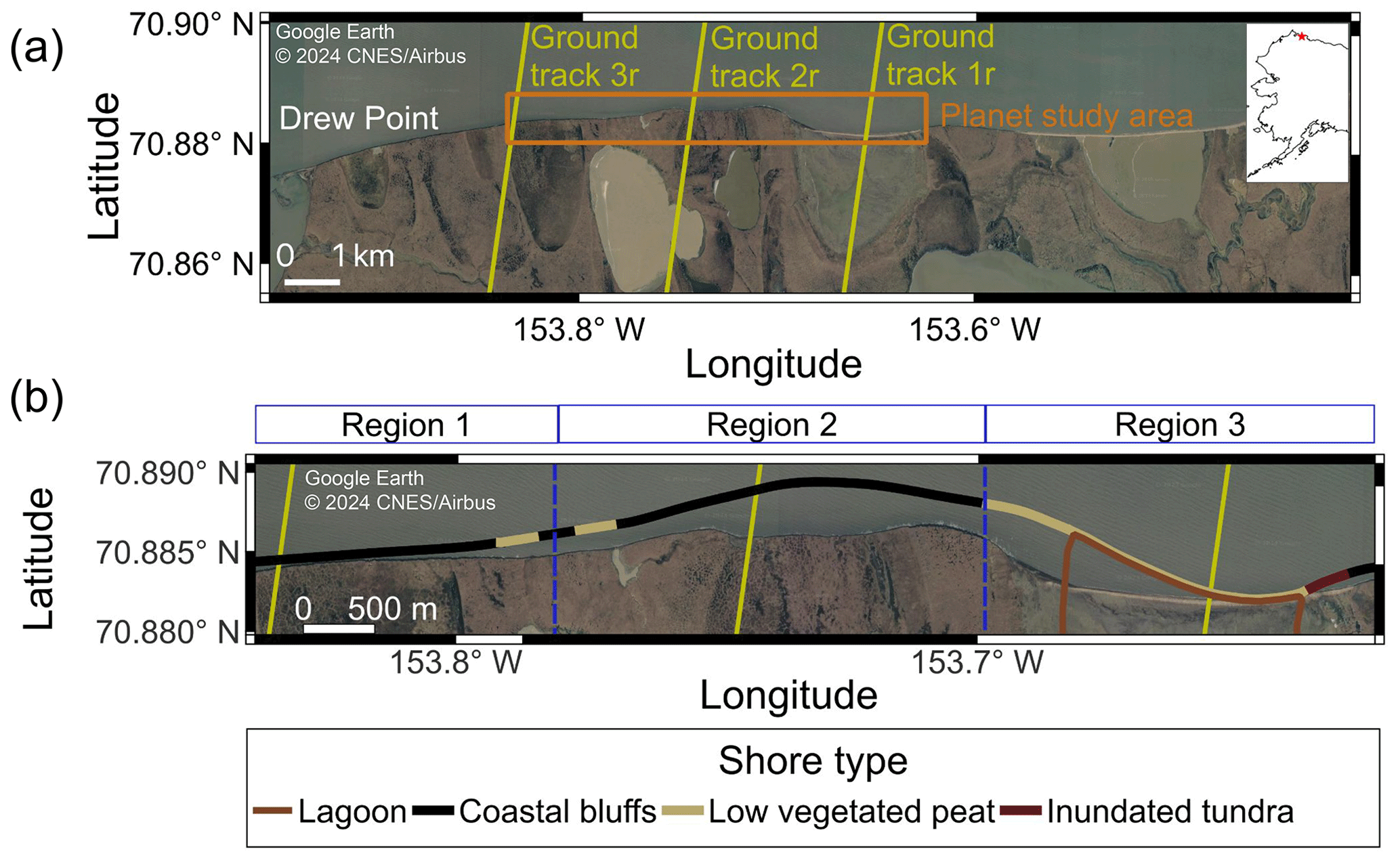
Figure 1 (a) Overview of the study area on the Alaskan Beaufort Sea coast, with the extent of the Planet imagery used and the locations of the ICESat-2 ground tracks indicated. (b) A close-up of the study area and shore-type classifications of the 2007 shoreline from ShoreZone (Harper and Morris, 2014). We divide our study area into three regions based on geography and shoreline type. Background imagery is from 2018, © 2024 Google Earth CNES/Airbus.

2 Data and methods

2.1 Study area

Our study focused on an 8 km stretch of coast to the east of Drew Point on the North Slope of Alaska (Fig. 1). This study area largely consists of exposed ice-rich bluffs with narrow beaches along the coast and thermokarst lakes and drained lake basins onshore (Jorgenson et al., 2014; Gibbs and Richmond, 2015). Most of the shoreline in this region is less than 3 m high, although the bluffs near Drew Point reach as high as 6 m (Gibbs and Richmond, 2015). Erosion is largely driven by thermal mechanical notching of bluffs, followed by bluff collapse (Barnhart et al., 2014; Gibbs and Richmond, 2015; Jones et al., 2018). The area around Drew Point is among the most rapidly retreating locations in the Arctic, with decadal-scale shoreline change rates in excess of −10 m a⁻¹ (Jones et al., 2009; Gibbs and Richmond, 2015) and evidence that retreat rates are increasing in recent years (Jones et al., 2009, 2018). Jones et al. (2018) found highly variable change in this study area, with mean shoreline change averaged over a 9 km stretch of shoreline varying from −6.7 to −22.0 m per open-water season between 2007 and 2016. Although they found that the greatest retreat occurred in the year with the most storms and the warmest air temperatures, they did not find a robust relationship between spatially averaged retreat rates and open-water days, storm activity, air temperature, permafrost temperature, or sea surface temperature over the entirety of the 10-year study period. Maximum local retreat was 2–3 times higher than spatially averaged retreat, pointing to the potential influence of local controls (such as morphology) on shoreline change.

We divide our study area into three regions (Fig. 1b.) with repeated cross-shore ICESat-2 profiles. We delineate these regions primarily based on visual analyses of 2018 optical imagery collected by CNES Airbus that was accessed through Google Earth and draw on Gibbs and Richmond (2015), Jones et al. (2009), and the ShoreZone database (Harper and Morris, 2014; Alaska ShoreZone, 2023) to describe the morphological setting of each region. ShoreZone includes a classification of variable-length segments of the shoreline based on aerial photography taken in 2007. These classifications are based on the substrate and morphology of the shoreline as well as the dominant erosion and accretion processes thought to be present. Given the high amount of shoreline retreat in the last decade (Jones et al., 2018), specific local features identified by ShoreZone in 2007 may have been removed or modified, but we expect the general morphologic setting to be consistent with current conditions. Region 1, the westernmost portion of the study area, primarily consists of steep, ice-rich coastal bluffs (Jones et al., 2009; Harper and Morris, 2014; Gibbs and Richmond, 2015). ShoreZone indicates the sporadic presence of low, vegetated peat-rich sediment, which is likely the remnants of old drained lake basins (Jones et al., 2009) that have since been removed by erosion. Region 2 consists of the headlands and is characterized as having the same shoreline types as Region 1 (coastal bluffs and drained lake basins). Region 3 is a large breached thermokarst lake (Jones et al., 2009; Gibbs and Richmond, 2015) that is classified in ShoreZone as a large lagoon behind a narrow strip of low vegetated peat. The easternmost portion of this shoreline is classified as an inundated tundra environment, where the nearshore elevation is below sea level and where there has been significant thaw subsidence and flooding.

2.2 Time-varying environmental conditions

To investigate the drivers of year-to-year variations in shoreline positions, we considered ocean wave conditions, air temperature, and sea ice concentration from the European Centre for Medium-range Weather Forecasts Reanalysis v5 (ERA5) dataset (Hersbach et al., 2020; Hersbach et al., 2023). ERA5 provides hourly estimates of atmospheric and sea ice conditions at a 0.25° resolution and wave conditions at a 0.5° resolution.

2.2.1 Sea ice and ocean waves

During the open-water season, waves transport heat and mechanical energy to the base of permafrost bluffs, driving retreat via thermal and mechanical abrasion (Aré, 1988; Wobus et al., 2011; Baranskaya et al., 2021). The vast majority of shoreline retreat along the Beaufort Sea coast occurs during the open-water season, and the length of the open-water season has been proposed as first-order predictor of retreat rates (Overeem et al., 2011). For each year, we estimated the duration of the open-water season from the ERA5 daily mean sea ice concentration. Following Overeem et al. (2011), we defined the open-water season as the period over which the daily mean sea ice concentration is < 15 %. The open-water season spans the period starting from the first day sea ice concentration falls below 15 % for at least 2 consecutive days to the first day sea ice concentration remains above 15 % for at least 2 consecutive days. We also counted the total number of open-water days (owds) spanned by each pair of Planet and ICESat-2 acquisitions, including single-day breakup events that occur outside of the open-water season.

The majority of wave-driven retreat is thought to occur during storms with large waves (Barnhart et al., 2014), although time lapse imagery has shown that thermal erosion and bluff collapse can occur even under relatively calm conditions (wave heights < 0.3 m) as long as waves make contact with the base of the bluffs (Overeem et al., 2011; Wobus et al., 2011). Thus, we considered both the frequency of extreme wave events and total wave exposure over the open-water season. We calculated the integral of the squared hourly significant wave height (H_s) as a proxy for cumulative wave energy. We defined the count of extreme events as the number of hours for which H_s≥1.4 m, corresponding to the upper 5 % of wave heights over the 3-year study period.

2.2.2 Air and sea surface temperature

Ocean temperatures are an important driver of thermal mechanical erosion, as warm temperatures are required to melt frozen sediments, which are then removed by waves. Modeling of ice-rich bluffs by Barnhart et al. (2014) showed that large retreat events only occur when ocean temperatures exceed 0 °C. Subaerial retreat, which drives the loss of sediment from the upper shoreline via permafrost thaw, is driven by warm air temperatures (Wobus et al., 2011; Barnhart et al., 2014; Baranskaya et al., 2021).

We aggregated daily mean air temperature from ERA5 between 1 June and 31 October of each year (following Jones et al., 2018) and the daily mean sea surface temperature for each open-water season, when the base of the shoreline is exposed to the ocean. For both the air and sea surface temperature for each measurement period, we calculated the number of accumulated degree days of thaw (ADDT), defined as the sum of daily temperatures >0 °C. We also recorded the mean air and ocean temperature between 1 June and 31 October of each year.

2.3 Shoreline identification from satellite multispectral imagery

We estimated annual shoreline positions using 3 m multispectral (red, green, blue, and near-infrared) images from Planet Labs' Super Dove, Dove R, and Dove Classic satellite constellations (Planet Team, 2023). We used four images, each collected near the beginning of each open-water season from 2019 to 2022 (Table 1, Fig. 2). Frequent cloud cover in 2019 necessitated the use of imagery from 25 June, when a small amount of snow or ice remained visible near the shoreline.

Historically, shoreline change has been estimated from satellites via manual delineation of the shoreline (Günther et al., 2015; Farquharson et al., 2018; Jones et al., 2009; Irrgang et al., 2018). Recent workflows such as CoastSat (Vos et al., 2019) have been developed to automatically detect the shorelines at a subpixel resolution, but they have focused on lower-latitude beaches and may not perform well in Arctic regions where sea ice is present. Here, we implement our own shoreline detection method, following some of the same steps as Vos et al. (2019). For each image, we calculated the normalized differenced water index (NDWI) from the green (G) and near-infrared (NIR) bands:

$$\begin{array}{}\text{(1)}& {\displaystyle }\mathrm{NDWI}={\displaystyle \frac{\mathrm{G}-\mathrm{NIR}}{\mathrm{G}+\mathrm{NIR}}}.\end{array}$$

We identified the NDWI threshold corresponding to the land–water boundary using Otsu's method, which determines the threshold that divides a set of pixels into two classes such that the interclass variance is maximized (Otsu, 1979) (see the histograms in Fig. A1). We identified the subpixel land–water boundary from our NDWI images using a marching squares algorithm implemented in matplotlib contour in Python (Hunter, 2007). We found that calculating our threshold using all image pixels resulted in an adequate shoreline estimate for all four of our images, such that an initial identification of land and water pixels (as is done in Vos et al., 2019) is not necessary. We visually identified and masked out regions where the shoreline appeared to be misidentified due to an ambiguous land–water boundary (shaded regions in Fig. 3). In order to improve the visual agreement of the derived shorelines with the visible shoreline in imagery and to ensure regular along-shore sampling intervals, we smoothed each shoreline using a 30 m along-shore running mean and sampled every 10 m alongshore to produce our final shoreline segments (Fig. 2). Finally, we estimated shoreline change using an approach similar to that of the USGS Digital Shoreline Analysis Software (Himmelstoss et al., 2021). In this workflow, a reference shoreline (hereafter referred to as the baseline) is selected. Cross-shore transects are generated at regular intervals along-shore that are perpendicular to this baseline. The change between consecutive shorelines is then calculated along these transects. We created a baseline by smoothing the raw 2020 shoreline with a 60 m along-shore running mean in order to make sure that adjacent cross-shore transects did not intersect on the time interval of our study site. Transects were generated every 10 m along the baseline using a modified version of the SDS_transects routine from the CoastSat Toolbox (Vos et al., 2019; Vos et al., 2024), which generates transects that bisect the shoreline. The change along each transect was calculated between each successive shoreline.

The estimated shorelines are subject to uncertainty from image geolocation errors, tidal- and storm-driven wave runup influences on the land–water boundary, and errors in the threshold determined with Otsu’s method. The tides in this region tend to be less than 0.2 m, but storm surges can result in temporary relative sea level increases of up to 1.4 m (Jones et al., 2018). However, given that much of this region consists of steep bluffs with narrow or no beaches (Gibbs and Richmond, 2015), changes in the local relative sea level are not expected to have a large impact on the observed land–water boundary. To estimate the uncertainty in our shoreline estimates, we identified six clusters of three to six images (25 images in total) taken within a week of one another in the early summer (mid June through late July). Modeling of coastal bluff retreat in this region by Barnhart et al. (2014) suggests that large (> 2.5 m) retreat events are concentrated in late summer (late July–late September) and driven by storms. Therefore, we do not expect large retreat events during early summer, such that the dominant source of change over short periods will be transient signals, such as relative sea level changes and geolocation offsets. We calculated the cross-shore difference between each shoreline position and the mean position of its cluster and pooled the residuals across all shorelines (Table A1). We defined our shoreline estimation uncertainty to be the standard deviation of the pooled residuals.

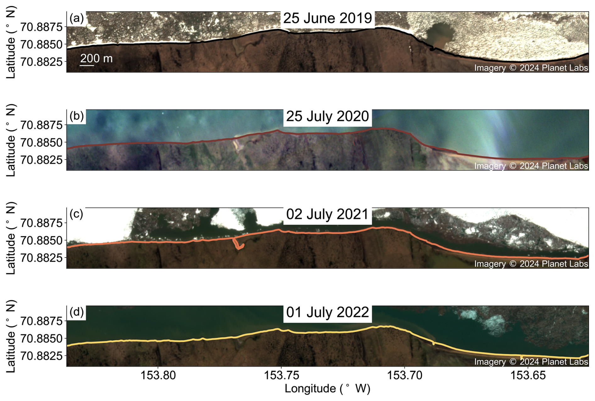
Figure 2 Planet Labs imagery (© 2024 Planet Labs Inc) used to estimate shoreline positions. Shorelines delineated using Otsu thresholding are overlain and show good agreement with the visible land–water boundary.

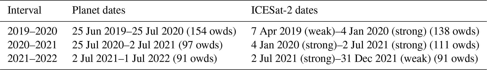
Table 1 Observation intervals from Planet imagery and ICESat-2. The number of open-water days (owds) spanned by each acquisition is listed in parenthesis.

2.4 Elevation profiles from ICESat-2 altimetry

Outside of the poles, the majority of ICESat-2 revisits between 2019 and 2022 were off-pointed from their nominal ground track location to increase aerial coverage, such that subsequent revisits did not cover the same ground location. However, “target of opportunity” requests over the North Slope of Alaska resulted in exact repeats of every fifth descending reference ground track starting in April 2019. We analyzed repeat ICESat-2 elevation profiles from three ground tracks (ground tracks 3r, 2r, and 1r, labeled in Fig. 1a) from a single reference ground track crossing our study area. Due to frequent cloud cover in the summer and fall, as well as the relatively low surface reflectivity of the snow-free tundra, the majority of observation dates with sufficient surface-reflected photons to accurately identify the surface occurred in the winter (January and April), with 2021 being the only year with snow-free profiles available. We selected four observation dates spanning the 2019–2021 open-water seasons (Table 1), resulting in 12 individual profiles.

For each profile, we used 200 m of cross-shore ATL03 photons (Neumann et al., 2023) for our analysis. Each photon from ATL03 is assigned a confidence code ranging from 0 (noise) to 4 (high confidence) to indicate how likely it is to be a transmitted photon that was reflected from the surface (i.e., a signal photon). From each ATL03 profile, we selected all high-confidence (confidence score = 4) and medium-confidence (confidence score = 3) photons for further processing. These photon data were plotted and inspected to provide a qualitative analysis of small-scale features. We used the SlideRule Python client (Shean et al., 2023) to run a customized version of the ATLAS/ICESat-2 L3A Land Ice Height (ATL06) algorithm (Smith et al., 2019), which estimates surface elevations using an iterative process of filtering and linear fitting of individual photon elevations. In this process, a linear fit is performed over fixed-length along-track segments of signal photons, outliers are filtered out based on a specified window above and below the linear surface, and the remaining photons are refit. This process is iterated using a successively narrower outlier window until either it converges or the outlier window reaches a user-specified minimum value. The reported elevation for each segment is the height of the midpoint of the final linear interpolation. SlideRule provides the root-mean-square (RMS) error between the photons used in the final fitting and the final linear fit, as well as the photon-level elevation error that is propagated through the linear fit. The photon elevation error is assumed to be uniform for a given segment and is estimated as the maximum of the segment's RMS error and the robust spread of photons as defined by Smith et al. (2019). This robust spread is based on the vertical distribution of signal photon heights and the estimated rate of background photons (i.e., photons that are not surface signals).

For coastal applications, a high along-track resolution is preferable to capture abrupt elevation changes at the shoreline. However, shorter segments may not provide enough photons for a robust linear fit and may result in height estimates that are subject to along-track variations in photon density. A longer segment length results in a smoother profile at the cost of not capturing small-scale features. In order to strike a balance between these two considerations, we implemented the SlideRule ATL06 algorithm for 10 m long segments spaced every 2 m along track, such that consecutive segments overlapped by 80 %. A 10 m section was only considered valid if it contained at least five signal photons and if those photons were distributed over at least 1 m along track. Bright surfaces such as surface ponds can lead to after pulses in the ATL03 data, which appear as secondary surfaces starting ∼ 0.45 m below the true surface (Lu et al., 2021; Arndt and Fricker, 2024). The original ATL06 algorithm sets the minimum height of the outlier window to 3 m, which leads to the inclusion of these after pulses in the final surface elevation estimate. To avoid including after pulses in our analysis, our custom ATL06 processing allows for an outlier window height as narrow as 0.80 m (i.e., 0.4 m above and below the identified surface).

To estimate shoreline change from our custom ICESat-2 elevation profiles, we needed to reliably identify shoreline boundaries from the derived elevation profiles. The presence of sea ice and snow in three of the ICESat-2 tracks prevents the accurate identification of a land–water boundary. Instead, we identified the boundaries of the backshore, defined here as the relatively steep region between the beach or ocean and the onshore region. We manually identified the point corresponding to the backshore–onshore boundary (henceforth referred to as the “upper shoreline”) and backshore–offshore boundary (the “lower shoreline”) based on the visual breaks in the along-track slope (see Fig. A2). Since beaches in this region are very narrow when present (Gibbs and Richmond, 2015), we expect the lower shoreline from ICESat-2 to be similar to the land–water boundary. We identified the intersection between each ICESat-2 track and the corresponding imagery-derived shoreline and compared the shoreline positions and cross-shore retreat estimates derived from Planet and the two ICESat-2 boundaries. Under the assumption that the majority of the observed position change in our ICESat-2 boundaries is due to cross-shore change, we projected our ICESat-2-derived change estimate in the local cross-shore direction. The local cross-shore vector was based off of the baseline transect (as defined in Sect. 3.2) that was located closest to the geographic midpoint of the four ICESat-2 transects associated with each ground track.

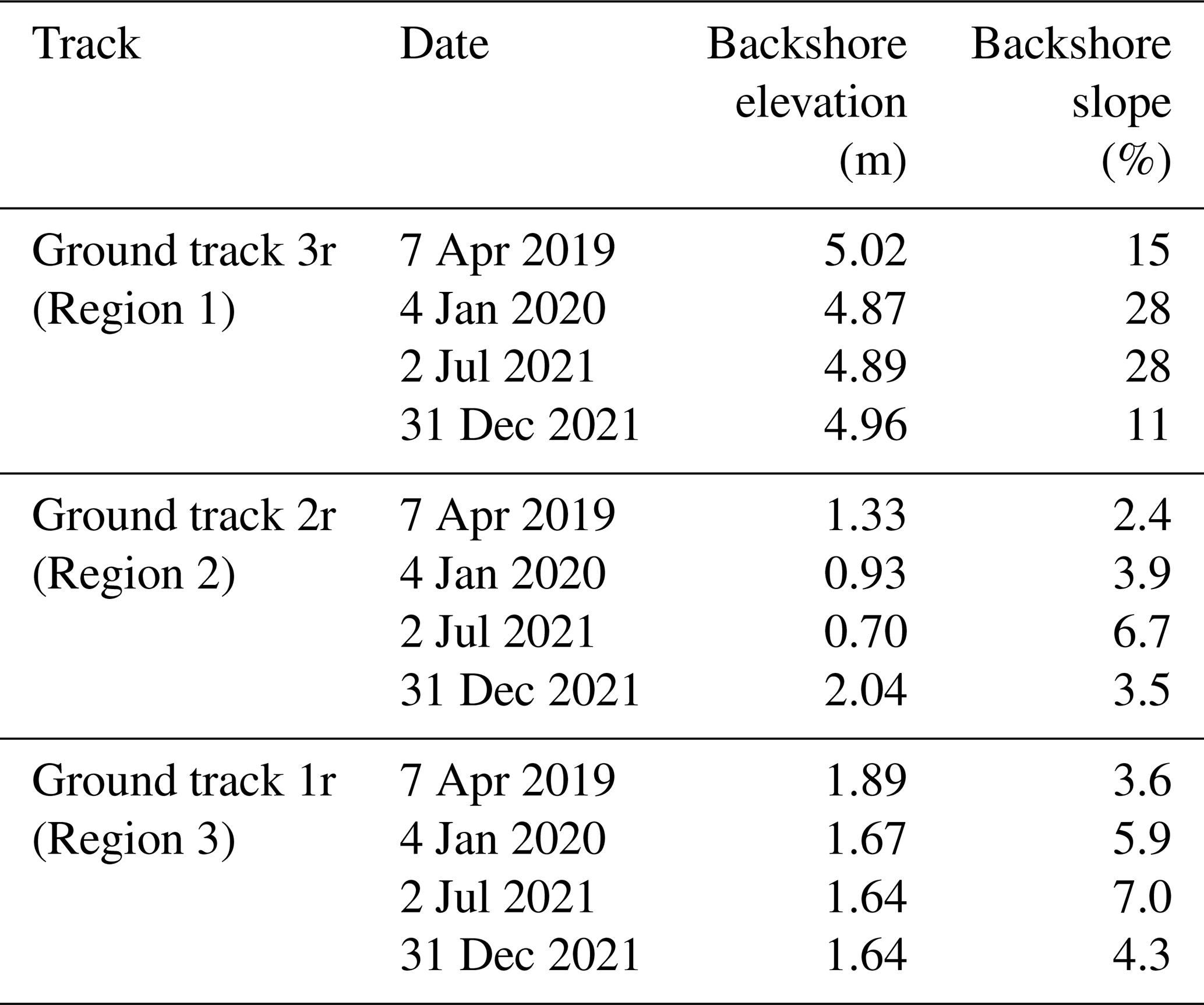
In order to characterize the morphology of each profile, we calculated both the backshore elevation and the backshore slope. The backshore elevation was defined as the elevation difference between the backshore–onshore boundary and the mean offshore (north of the backshore–offshore) elevation from the 2 July 2021 elevation profiles, which we used as a proxy for local sea level (illustrated in Fig. A2). The backshore slope was estimated using a linear fit of all points between the backshore–onshore and backshore–offshore boundaries, projected into the local cross-shore direction.

To estimate the uncertainty in our ICESat-2-derived boundaries, we use the geolocation uncertainties estimated by Luthcke et al. (2021), who coregistered ATL03 data with ArcticDEM and reported the distribution of offsets between the original and shifted locations for each beam. We consider the total uncertainty, defined as the mean offset plus 1 standard deviation for each beam. This total uncertainty ranges from 2.8 to 4.8 m for individual beams. We consider the worst-case scenario where this error is entirely in the cross-shore direction. The satellite performs a “yaw flip” twice every 502 d where it is reoriented by 180° (Luthcke et al., 2021). This means that the specific beam sampling a given ground track, and therefore the associated geolocation uncertainty, alternates between repeats. We take the uncertainty in the shoreline change between two observation dates as the sum in quadrature of the uncertainties in the individual measurements and find that they range from 4.0 to 5.9 m.

3 Results

3.1 Environmental conditions

We observed the most extreme environmental conditions as measured by all measured metrics in 2019 (Table 2). The 2019 erosion year had the longest open-water season, with sea ice breaking up sooner (late June) and re-forming later (mid-November) than in the other 2 years. It also had the highest wave energy, the most storms, highest air temperatures, and over twice as many ocean thawing degree days as the following 2 years. By contrast, the 2021 open-water season was the shortest, with sea ice breakup occurring in late July (although ERA5 suggests a 1 d ice breakup on 27 June) and freeze-up occurring in late October. There were slightly warmer ocean and air temperatures but lower wave activity (in terms of both wave energy and hours of high waves) in 2021 compared to 2020.

Table 2 Summary of environmental variables from ERA5 (Hersbach et al., 2020).

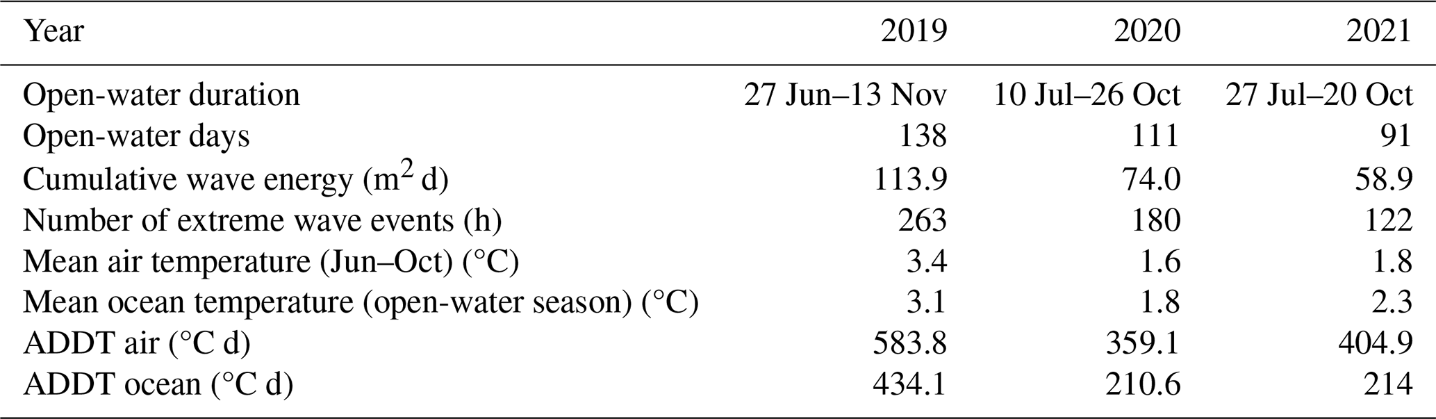
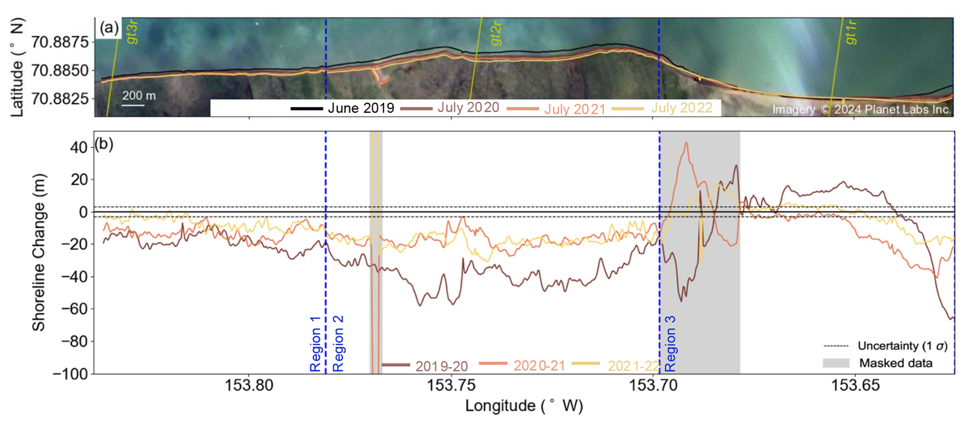
Figure 3 (a) Shorelines derived from Planet images, overlain on imagery from 25 July 2020 (© 2024 Planet Labs Inc). The locations of the three ICESat-2 ground tracks are also shown. (b) Cross-shore shoreline change calculated between successive years. Areas where there was an ambiguous land–water boundary are masked out (shaded areas) and excluded from analysis. The boundaries of the three regions shown in Fig. 1 are shown as dashed lines.

3.2 Imagery-derived shoreline position and retreat rates

The spatially averaged shoreline change rate in our study area was −16.5 m a⁻¹ (corresponding to retreat) between 2019 and 2021, with notable year-to-year and local variability (Table 3, Fig. 3). The year 2019 had the most shoreline loss, with a mean shoreline change of −23.7 m and single-segment (i.e., 10 m scale) shoreline change values as extreme as −66.7 m. The year 2020 experienced more moderate shoreline change, with a mean shoreline change of −15.4 m (ranging from −41.0 to +6.0 m). The year 2021 experienced similar but slightly lower rates, with a mean shoreline change of −10.5 m (−30.9 to +5.6 m).

Based on the uncertainty estimation described in Sect. 2.3, we estimated the precision of our shoreline position estimates to be 2.2 m. Assuming that the error in each shoreline is independent of the others, this corresponds to a position change uncertainty of 3.1 m. We define substantial shoreline change as any value that exceeds this threshold.

Table 3 Estimated shoreline change between each successive image observation date in each of the three regions identified in Fig. 3, as well as across the whole study area. The mean and range are listed.

Our shoreline change estimates for each region (Table 3, Fig. 3b) indicate that there was spatial variability between regions. Region 1 showed high retreat, with a mean change rate of −12.9 m a⁻¹ over 3 years and single-segment year-to-year shoreline change estimates ranging from −29.4 to +1.6 m. Shoreline change consisted almost exclusively of retreat, with the maximum observed advancement (+1.6 m) falling below our estimated uncertainty threshold (3.1 m). We observed the greatest spatially averaged retreat in 2019 (−18.5 m) and the lowest in 2021 (−7.1 m). While every shoreline segment in Region 1 underwent retreat in 2019 and 2020, 16 % of valid shoreline segments (all in the western half of Region 1) did not exhibit substantial (> 3.1 m) shoreline change in 2021.

Region 2 exhibited the largest overall retreat, with a 3-year spatially averaged mean change rate of −24.3 m a⁻¹ and year-to-year single-segment change estimates ranging from −58.2 to −3.0 m. As with Region 1, we observed the largest amount of shoreline change in 2019 (−38.4 m), with similar and smaller change in 2020 (−16.8 m) and in 2021 (−17.7 m).

Region 3 exhibited the smallest amount of shoreline change, with a 3-year spatially averaged rate of −6.0 m a⁻¹. Region 3 was the only region in our study area where substantial shoreline advance (up to +18.6 m locally in 2019) occurred. Although 2019 was not the year with the highest spatially averaged shoreline change (−0.6 m) in Region 3, it was the most dynamic year, with both the maximum observed local retreat (−66.7 m of shoreline change) and advance (+18.6 m of shoreline change). We found that 24 % of valid shoreline segments, concentrated almost exclusively in the easternmost third of the region, underwent significant retreat, whereas the central 62 % of shoreline segments experienced substantial advance. The remaining 14 % did not exhibit substantial retreat or advance. In 2020, the mean shoreline change across the region was higher (−13.5 m), but the change at individual segments was lower in magnitude (with a local maximum of −41.0 m) and spread over a larger area (the eastern 66 % of the basin). Only 3 % of shoreline segments showed substantial advance, whereas the remaining 31 % experienced no significant change. Relative to 2020, retreat in 2021 was lower in magnitude (with a maximum shoreline change of −20.7 m) and present across less of the region (40 %), resulting in a lower spatially averaged shoreline change (−3.9 m), with 19 % of segments showing significant advancement (with a maximum of +5.6 m) and the remaining 41 % experiencing no significant change.

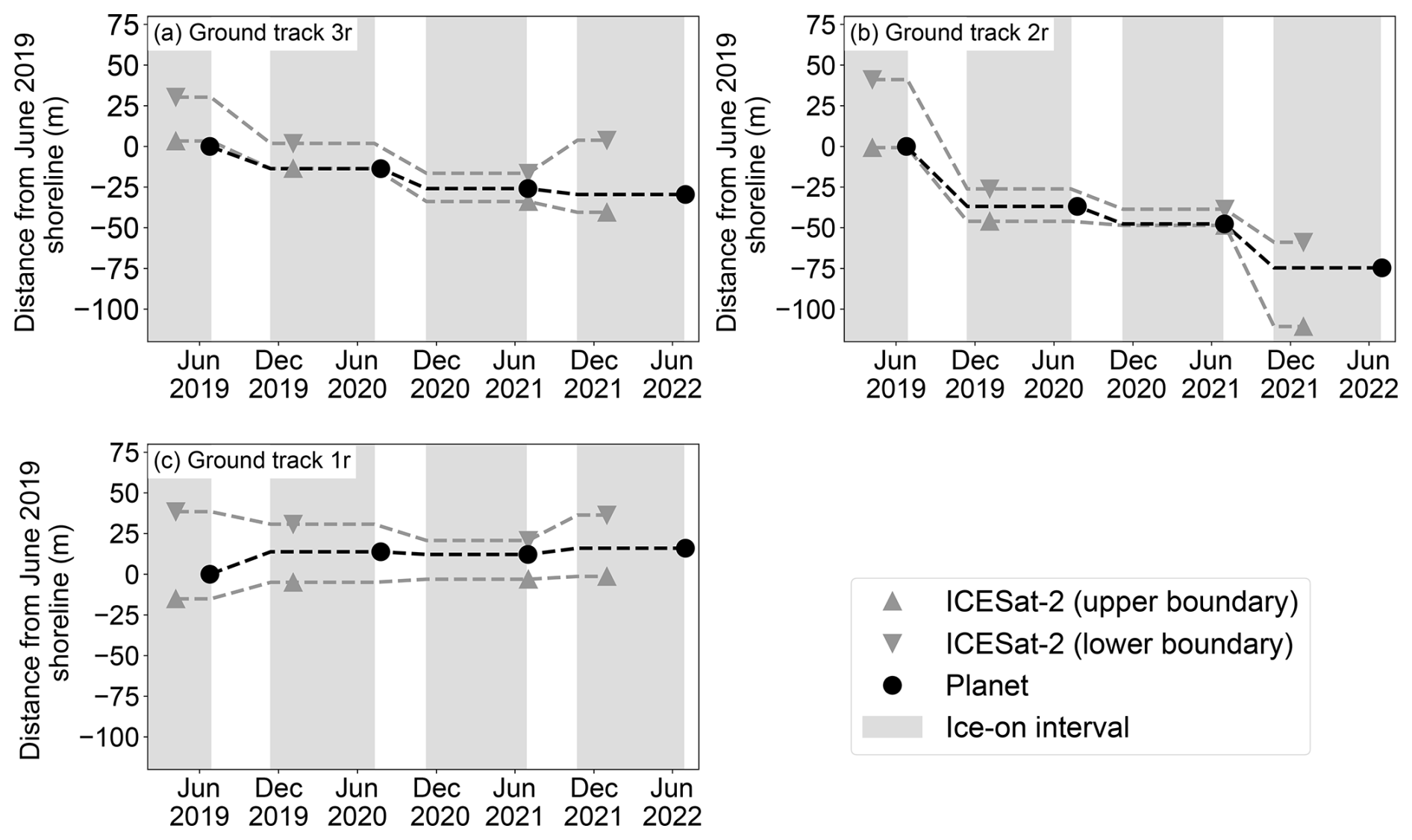
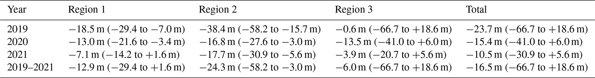
Figure 4 Time series of the positions of the upper and lower boundaries and coastal boundaries from ICESat-2 and the land–water boundary derived from Planet. Positions are given as the cross-shore distance from the Planet-derived shoreline from 25 June 2019. Ice-on intervals are shaded. Dashed lines indicate the trajectory of the shoreline based on a linear rate of change during the open-water season and no change during ice-on periods.

Figure 5 (a) Comparison between shoreline change estimates from Planet and shoreline change estimates from the upper (orange) and lower (blue) boundaries derived from ICESat-2. (b) Comparison between the measured change between each open-water season across the upper and lower boundaries derived from ICESat-2. The coefficient of determination excluding the outlier drained lake measurement (gray) is reported. Linear fits were estimated using orthogonal distance regression. A 1–1 line is shown for reference.

3.3 Cross-validation of ICESat-2 altimetry and Planet-imagery-derived shoreline positions

Altimetry from ICESat-2 provides an independent estimate of shoreline change at multiple positions along the shoreline profile, which can be compared to Planet-derived shoreline positions for validation. We find that overall shoreline positions estimated from both datasets are consistent. We would expect the land–water boundary from Planet to be located seaward (north) of the lower backshore boundaries identified by ICESat-2. However, we found that the Planet-derived land–water boundary consistently falls landward (south) of the ICESat-2-derived lower boundary (by 8.6 ± 4.2 to 41.1 ± 4.5 m) and either seaward (by up to 36.0 m ± 4.5 m) or slightly landward of the ICESat-2-derived upper boundary (by up to 3.3 ± 4.0 m) (Fig. 4), such that it is located on the backshore or onshore section of the elevation profiles. Given the published geolocation errors from ICESat-2 (up to 4.8 m; Luthcke et al., 2021) and Planet (< 10 m; Planet Team, 2023), the difference between ICESat-2- and Planet-derived shorelines is not thought to be due to a consistent geolocation offset between the two satellite estimates. The difference could be explained by a consistent landward bias in our NDWI thresholding technique (Sect. 2.3) or by differences introduced by snow cover and variations in the local water level. Although observations from ICESat-2 and Planet span different time intervals (Table 1, Fig. 4), the number of open-water days spanned by both are similar, allowing for a direct comparison between our imagery and altimetry-defined shoreline change estimates. We perform an orthogonal distance linear regression and find a high correlation between the Planet-derived change estimates and changes in the ICESat-2-derived upper boundary (r²=0.79, p=0.0008) and moderate correlation with changes in the ICESat-2-derived lower boundary (r²=0.52, p=0.007) (Fig. 5a).

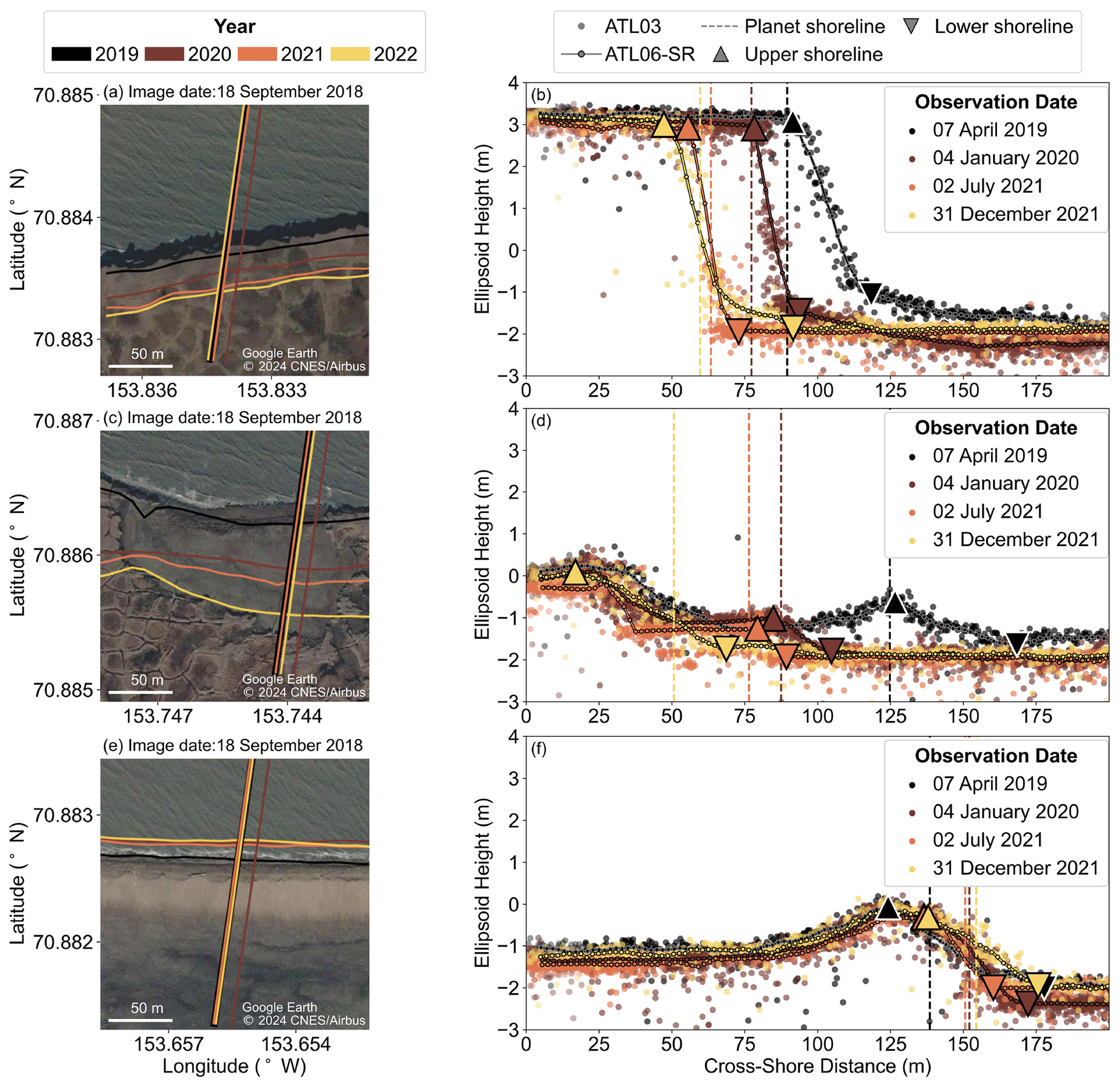
Figure 6 (a, c, e) Detailed view of the ICESat-2 sampling location from 2018 satellite imagery (© 2024 Google Earth CNES/Airbus) for (a) ground track 3r; (c) ground track 2r, and (e) ground track 1r. The location of the Planet shoreline and corresponding ICESat-2 pass for each year is shown. (b, d, f) ATL03 photon clouds from each ICESat-2 pass, with the SlideRule-derived (ATL06-SR) elevation profile overlaid on the photon clouds for (b) ground track 3r, (d) ground track 2r, and (f) ground track 1r. The estimated locations of the upper- and lower-shoreline boundaries for each date are marked, along with the cross-shore locations of the Planet-derived shorelines. The colors follow the same legend as (a), (c), and (e).

Table 4 Onshore heights and slopes derived from the upper and lower boundaries identified for each ICESat-2 observation.

3.4 Topographic change from satellite altimetry

Our SlideRule-derived elevation profiles (Fig. 6b, d and f) fit the ATL03 photon data well, with RMS errors ranging from 0.04 m to 1.3 m and a mean RMS error of 0.15 m (Figs. A3, A4, A5). The propagated vertical uncertainty ranges from 0.0024 to 0.27 m, with a mean uncertainty of 0.029 m. We now discuss the time evolution of the shoreline horizontal position (Table A2), backshore elevation, and backshore slope (Table 4) at each ICESat-2 ground track.

Ground track 3r in Region 1 (Figs. 6a, b, 4a) shows a coastal bluff (such as the one shown in Fig. A6a) that underwent retreat with little change in morphology. The upper- and lower-shoreline boundaries showed consistent retreat in 2019 and 2020, with cross-shore change at each boundary ranging from −16.9 to −28.4 m. During these 2 years, we observed a steepening of the backshore slope from 15 % in 2019 to 28 % in 2020 and 2021. In July 2021, we note a cluster of photons that is ∼ 1 m high and ∼ 5 m across at the base of the bluff (Fig. 7a) that may correspond to toppled bluff material. Between 2021 and 2022, we observed slight retreat of the upper boundary (−6.6 m of shoreline change) and advance of the lower boundary (+20.3 m), resulting in a reduction in the backshore slope to 11 %. In December 2021, we again note a ∼ 1 m high cluster of photons at the base of the bluff that gently slopes down towards the mean offshore height over ∼ 20 m (Fig. 7a). The backshore elevation remained stable, ranging from 4.89 to 5.02 m over the 3-year study period.

Ground track 2r (Figs. 6c, d, 4b) in Region 2 passes over the remnant basin of a ∼ 150 m diameter lake that was breached and drained as a result of shoreline retreat prior to our study. This profile underwent large changes in both the shoreline position and morphology. Aerial imagery from ShoreZone (Fig. A6b) showed the lake pre-drainage, and the lake basin was clearly visible in Airbus imagery from Google Earth (Fig. 6c) and in our 2019 ICESat-2 profile (Fig. 6d). Between 2019 and 2020, −45.3 m of upper-shoreline change and −67.2 m of lower-shoreline change occurred, corresponding to the loss of about half of the basin. This resulted in a 0.40 m drop in the backshore height, from 1.33 to 0.93 m, and an increase in the backshore slope from 2.4 % to 3.9 %. By contrast, between early 2020 and early 2021 there was almost no change in the upper-shoreline position (−2.5 m) and only moderate change in the lower-shoreline position (−12.5 m), resulting in a further increase in the backshore slope to 6.7 %. We also observed a slight lowering of 0.23 m of the backshore height. The photon distribution over the lake basin in July 2021 is concentrated in a narrow height band, with a secondary reflection below the surface (Fig. 7b). This feature is indicative of an after pulse due to surface ponding (Lu et al., 2021), suggesting the presence of shallow water. The rest of the lake basin was eroded between July and December 2021, resulting in −62.1 m of change in the upper shoreline and −20.3 m of change in the lower shoreline. This necessitated the definition of a new, substantially higher (2.04 m) backshore boundary and resulted in a shallowing of the backshore slope from 6.7 % to 3.5 %.

Ground track 1r (Figs. 6e, f, 4c) in Region 3 passes over a 1.71 m high dune in front of a ∼ 2.6 km wide breached thermokarst lake (shown in more detail in Fig. A6c) that showed little shoreline change relative to other regions. We observed between +1.7 and +10.2 m of advance in the upper boundary each year, while the lower boundary retreated in 2019 (−7.7 m) and 2020 (−10.0 m) and then advanced in 2021 (+15.6 m). We note a 0.22 m drop in the backshore elevation (from 1.89 to 1.67 m) between 2019 and 2020, after which the elevation remained stable from 2020 to late 2021 (1.64 to 1.67 m). The backshore slope steepened between 2019 and 2021, from 3.6 % to 7.0 %, and then relaxed to 4.3 % in late 2021.

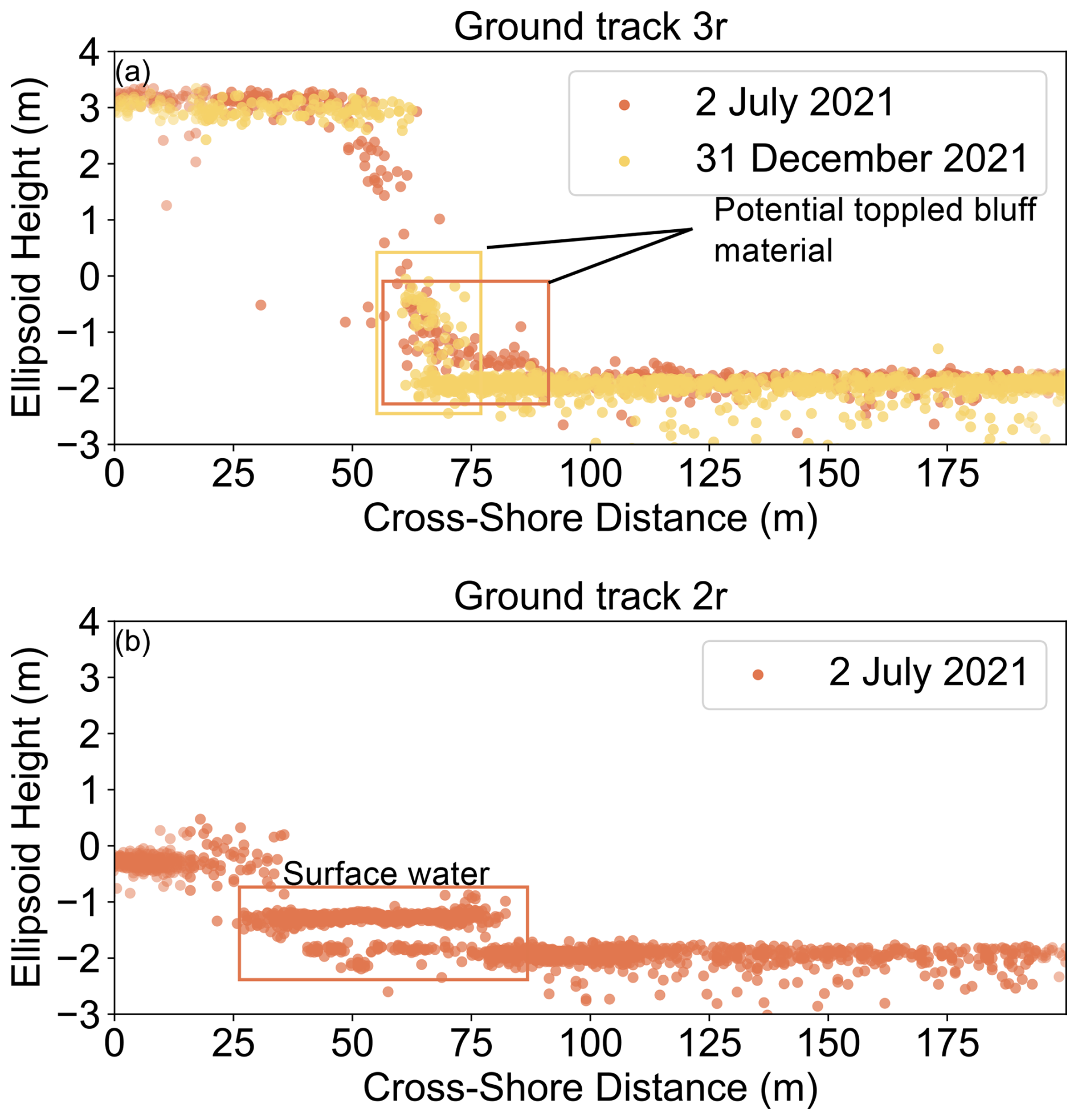
Figure 7 ICESat-2 ATL03 photon data show small-scale features, including (a) returns over what may be toppled block material at the base of the bluff at ground track 3r and (b) surface ponding in the drained lake basin at ground track 2r.

4 Discussion

4.1 Spatiotemporal variability in shoreline change in the context of previous observations

Our estimates of spatially averaged (regional) mean annual shoreline change (−10.5 to −23.7 m a⁻¹) across our study region are higher than long-term historical estimates and are similar to recent observations (Fig. A7). Gibbs and Richmond (2015) estimated a regional mean of −6.3 m a⁻¹ and a local maximum of −18.6 m a⁻¹ between Drew Point and Cape Halket between 1947 and 2002. Jones et al. (2009) estimated shoreline change across this region over multiple time intervals and found −6.8 m a⁻¹ of change between 1955 and 1979, −8.7 m a⁻¹ between 1979 and 2002, and −13.6 m a⁻¹ between 2002 and 2007. A follow-up study by Jones et al. (2018) estimating shoreline change over a 9 km region covering our study area found a 10-year mean shoreline change rate of −17.2 m a⁻¹ between 2007 and 2016. In addition to estimating a 10-year mean, Jones et al. (2018) reported regional year-to-year rates, which ranged from −6.7 to −22.6 m a⁻¹. Our mean retreat rates in 2020 and 2021 fall within the range of the year-to-year rates observed by Jones et al. (2018), whereas our mean retreat in 2019 (−23.7 m) slightly exceeds that range. Our 3-year mean of observed retreat rates (−16.5 m) is similar to the decadal-scale estimate from Jones et al. (2018) and is consistent with an increase in local shoreline change rates compared to 2002–2007 (Jones et al., 2009). Our retreat estimates and the post-2002 estimates of Jones et al. (2009) and Jones et al. (2018) are all higher than the pre-2002 decadal-scale estimates of Gibbs and Richmond (2015) and Jones et al. (2009). This increase could be reflective of a long-term increase in retreat rates, although it may also be due to differences in timescales between studies, as short-term estimates of shoreline change tend to be higher in magnitude than long-term estimates (Sadler and Jerolmack, 2015).

Previous observations suggest that the spatial distribution of change rates across our study area has been variable over time. Gibbs and Richmond (2015) found the highest rates of shoreline change in Region 3 (−10 to −18 m a⁻¹), intermediate rates in Region 2 (−8 to −12 m a⁻¹), and slightly lower rates in Region 1 (−6 to −12 m a⁻¹) between 1947 and 2002. Jones et al. (2009) found a similar pattern between 1955 and 1979, with the shoreline change in Region 3 occurring at rates in excess of −10 m a⁻¹ and shoreline change in most of Region 1 and Region 2 occurring at rates between −5 and −10 m a⁻¹. However, they found that shoreline change rates in Region 2 increased to be in excess of −10 m a⁻¹ between 1979 and 2002, and change rates in Region 1 followed suit between 2002 and 2007 such that change rates across the region were relatively uniform (averaging −18 m a⁻¹) between 2002 and 2007.

In contrast, our observed shoreline change rates between the three regions between 2019 and 2021 are not uniform. Although the relatively high rates of retreat we observed in Region 2 compared to Region 1 are consistent with Gibbs et al. (2019) and Jones et al. (2009), the stability of the central portion of Region 3 that we observed with both ICESat-2 altimetry and Planet imagery appears to be a recent development. Wang et al. (2022) sampled a transect across the central portion of Region 3 from satellite-imagery-derived shorelines from 1974, 1985, 1992, 2001, 2009, and 2017 and estimated a mean shoreline change rate over the full study period of −55.9 m a⁻¹. When considering the rates between successive shorelines, Wang et al. (2022) found that 2009–2017 was the only time interval during which there was no observed shoreline change, suggesting that stabilization occurred in this time frame after over 4 decades of retreat.

4.2 Drivers of spatiotemporal variability in imagery-derived shoreline change

Jones et al. (2018) found that the environmental drivers of year-to-year variability on the Beaufort Sea coast are not well-defined, but they did observe high retreat in years with extreme weather, which is consistent with our findings of both high retreat and extreme environmental conditions in 2019. Compared to 2020 and 2021, 2019 had a long open-water season and elevated air and ocean temperatures (Table 2), all of which likely contributed to the elevated spatially averaged retreat across the study region.

Although there is correspondence between mean year-to-year shoreline change and year-to-year variations in wave and temperature conditions, the response of the shoreline to these time-varying conditions is not spatially uniform (Fig. 3b). In 2019, Region 1 and Region 2 both experienced high retreat, while Region 3 underwent high retreat across parts of the shorelines and moderate advancement across others. While we do not expect air and ocean temperatures to vary greatly spatially over the study region, local variations in wave energy due to shoreline orientation, position, and morphology may contribute to the observed spatial variability. For indented shorelines such as our study area, wave energy is expected to be concentrated towards the headlands due to wave refraction, such that shorelines with uniform composition will straighten over time (Van Rijn, 2011). This provides a potential explanation for increased retreat in Region 2, particularly in 2019 when wave action was high. The year 2021 saw the lowest amount of wave energy and fewest storms (Table 2), and the concentration of wave energy in the headlands of Region 2 would result in particularly low wave energy in the hinterlands of Region 1 and Region 3. We note that while Region 1 and Region 2 both consist primarily of ice-rich coastal bluffs, the shoreline in Region 3 is characterized by ShoreZone primarily as low-lying peat (Fig. 1b.) that is expected to be subject to low incident wave energy (Harper and Morris, 2014). The eastern edge of Region 3 is characterized as inundated tundra, which refers to areas where thaw subsidence and surface ponding are present (Harper and Morris, 2014). Based on these characterizations and on our observed patterns of shoreline change, we posit that shoreline change in Region 1 and Region 2 is sensitive to year-to-year variations in wave energy and ocean and air temperatures, while the western and central portion of Region 3 are not. The eastern portion of Region 3 (inundated tundra) is likely subject to ground thaw, high wave energy, and flooding, resulting in high retreat in response to high wave activity and high temperatures. The advancement observed in Region 3 may be driven by along-shore transport of material lost from the surrounding regions.

4.3 Drivers of morphologic change observed from ICESat-2 altimetry

The elevation profiles from ICESat-2 data provide additional information on topographic and morphological change at specific ground tracks (Table 4), which can provide insight into specific erosion and accretion processes that drive local shoreline change. Specifically, we consider changes in backshore elevation, backshore slope, and relative change between the upper- and lower-shoreline boundaries.

Based on previous studies in the Beaufort Sea coast area (e.g., Overeem et al., 2011; Barnhart et al., 2014), we infer that the coastal bluff shown in ground track 3r in Region 1 (Fig. 6b) likely retreats primarily through the formation of thermal erosional niches, followed by bluff collapse. As the shoreline retreats, we observed no major morphological change; the backshore slope remained > 10 % with a stable (4.87 to 5.02 m) backshore elevation. However, there were year-to-year fluctuations in the backshore slope due to differences in change rates at the upper and lower boundaries of the backshore. In particular, the relatively low slope (11 %) in December 2021 is driven by a retreat of the upper boundary (−6.6 m of shoreline change) coupled with advance of the lower boundary (+20.3 m of shoreline change) (Table A2). Based on the ICESat-2 ATL03 photon data from July and December 2021 (Fig. 7a.), we hypothesize that this reduction in slope is due to the accumulation of collapsed bluff material at the base of the cliff that is not removed by the end of the 2021 open-water season. The low retreat derived from altimetry in 2021 is consistent with the low retreat estimated from Planet imagery in the broader Region 1 (which has a spatially averaged mean shoreline change of −7.1 m) and is possibly due to relatively low wave energy and fewer storms in the 2021 open-water season (Table 2). It may be that multiple locations along the shoreline in Region 1 observed in imagery were sheltered by un-eroded toppled bluff material similar to what we observe at ground track 3r.

The drained lake basin captured by ground track 2r in Region 2 (Fig. 6d) is an example of a more complex feature, which displays variable retreat as the shoreline migrates from the lake basin boundary to the bluff on the southern edge. The transition in shoreline morphology is reflected in an increase in backshore elevation from 0.70 to 2.04 m and moderate fluctuations in the backshore slope (2.4 % to 6.7 %; Table 4). The changes in slope between 2019 and 2020 and between early and late 2021 were driven by high and variable change (−20.3 to −67.2 m) in both the upper and lower boundaries, while the steepening of the slope between 2020 and 2021 was driven by the retreat of the lower shoreline (−12.5 m of shoreline change) and by little change in the upper shoreline (−2.5 m).

In order to assess whether the presence of this lake basin impacts local retreat rates, we compared the mean Planet-derived shoreline change across the drained lake basin (which spans 15 segments over 150 m) to the distribution of Planet-derived shoreline change across the entirety of Region 2. In 2019, the mean shoreline change across the lake basin (−35.3 m) is similar to the retreat in Region 2 overall, as it falls in the 63rd percentile of observed change. However, in 2020, shoreline change across the basin (−10.5 m) fell into the 8th percentile of observed headlands change, and in 2021 it was in the upper 90th percentile (−23.1 m). This suggests that the presence of the drained lake basin may have contributed to differential retreat during 2020 and 2021 relative to Region 2 overall. Differential retreat rates in drained lake basins have been observed before, with Jones et al. (2009) observing generally higher retreat rates of recently drained lake basins in this region between 1955 and 2002 relative to other land types (although this trend did not hold between 2002 and 2007). They suggested that the low elevation and presence of thawed sediments likely make drained lake basins more susceptible to erosion than coastal bluffs are. Our observation of surface water in July 2021 (Fig. 7b) is consistent with this interpretation, as it would help keep the underlying sediments in this basin thawed.

Based on our observations and the theory presented in Jones (2009), we can infer the processes driving the 3-year evolution of the drained lake basin. In 2019, wave-driven erosion of the seaward side of the drained lake basin exposed low-lying thawed sediments. In 2020, debris from this large erosion event may have sheltered the remainder of this basin, as evidenced by the retreat at the lower boundary and stability of the upper boundary. Once this debris was removed by waves, the low backshore elevation (0.70 m) would have left the basin susceptible to overtopping by high waves, and the thawed sediments would have had low mechanical strength, making the basin susceptible to rapid erosion, as was observed between early and late 2021. The steeper backshore slope in 2019 compared to in 2021 may have also contributed to increased wave runup (Earlie et al., 2018) and therefore increased mechanical erosion.

Both the upper- and lower-shoreline positions at ground track 1r in Region 3 (Fig. 6f, Fig. 4c) are relatively stable, whereas the other ground tracks exhibit high retreat. We see moderate advance (+10.2 m of shoreline change) and a drop in elevation (−0.22 m) of the backshore boundary in 2019 but very little change in either the position (+1.7 to +1.9 m, which falls within our estimated uncertainty) or elevation (which ranges from 1.64 to 1.67 m) of the backshore over the next 2 years. Fluctuations in the slope between observation dates are driven primarily by changes in the lower boundary (which undergoes between −10.0 and +15.6 m of shoreline change per year), which is consistent with sediment deposition and removal at the beach in front of the lagoon or changes in snow cover.

In order to understand the relative rates of retreat at the upper and lower boundaries of the shoreline, we perform an orthogonal distance regression between the annual change at both boundaries (Fig. 5b). We exclude change for the drained lake basin between July and October 2021, where the collapse of the remaining lake basin necessitated the definition of a new upper-shoreline boundary. We find a moderate correlation between upper- and lower-shoreline boundary change (r²=0.63, p=0.009) and a slope of 0.59 in the linear fit. Thus, both boundaries exhibit comparable amounts of change, but the lower shoreline (the interface between the backshore, beach, and ocean) is more dynamic.

4.4 Potential and challenges of using ICESat-2 for shoreline characterization

Analyses of both the geolocated photon data and the elevation profiles derived from ICESat-2 provide valuable insight into shoreline change. ICESat-2's geolocated photon product resolves coastal topography with a high level of detail, capturing abrupt elevation changes over horizontal distances of 5 m or less (e.g., Fig. 6b). We observe process-scale features such as toppled blocks and surface ponds in snow-free ICESat-2 profiles (Fig. 7). We find that the simplified elevation profiles derived via SlideRule can adequately capture the shoreline for the assessment of shoreline evolution, although small-scale features such as the toppled block on ground track 3r (Fig. 7a) and surface ponding on ground track 2r (Fig. 7b) are lost. ICESat-2 profiles allow for the identification of multiple shoreline boundaries, which can be compared against imagery-derived shoreline positions (Figs. 4, 5a). Furthermore, analysis of morphologic parameters such as backshore height and backshore slope can provide insight into specific erosional and accretional processes, such as the collapse of the small drained lake and the presence of toppled blocks at steep coastal bluffs.

The highest RMS misfits between the SlideRule-derived elevation profiles and underlying photons occur in areas with steep slopes and abrupt elevation changes (Figs. A3, A4, A5). This is particularly apparent for ground track 3r (Fig. A3), where the upper-shoreline boundary inferred from SlideRule often appears 2 to 5 m southward of the boundary that would be visually inferred from ATL03. The 10 m section length we used in SlideRule is likely too coarse to adequately capture abrupt elevation changes, but a shorter segment length would have relied on fewer photons per segment and would therefore have been more sensitive to variations in along-track photon density. An adaptive approach based on local topography and photon density may be able to capture steep and complex features more accurately.

Given the seasonal revisit time of ICESat-2 over our study region, the high frequency of cloud cover in the summer and fall, and the low reflectivity of the snow-free tundra, the majority of usable ICESat-2 data occurs in winter and spring, when snow and sea ice are present. Snow cover will impact ICESat-2-based shoreline position estimates, particularly the location of the lower-shoreline boundary, which will in turn impact our slope estimates. Although we expect the magnitude of snow-cover-induced changes to be small relative to the large retreat events observed at ground track 3r (the coastal bluff) and ground track 2r (the small drained lake), they may be the dominant source of change in areas with lower rates of change, such as ground track 1r (the large breached lake). Future work comparing snow-on ICESat-2 tracks to snow-off ICESat-2 tracks and snow-off digital elevation models could help quantify snow distribution at the shoreline and its impact on shoreline position estimates. There is also up to 15 m of horizontal offset between repeat ICESat-2 profiles (Fig. 6a, c, e), meaning that differences in shoreline position may in part be due to different sampling locations.

5 Conclusions

We used multispectral imagery from Planet and altimetry data from ICESat-2 to highlight spatiotemporal variability in changes in the position and topography of the shoreline along a dynamic section of the Beaufort Sea coast near Drew Point, Alaska, USA. We found kilometer-scale variability in annual shoreline change that reflects the response of distinct geomorphic units to time-varying wave and temperature conditions and small-scale variability (∼ tens of meters) that may be influenced by local shoreline morphology. We used elevation profiles from ICESat-2 altimetry to track changes in the position, elevation, and cross-shore slope of the shoreline at three ground tracks. We found that each ground track samples a distinct shoreline type that is subject to different mechanisms of change. At ground track 3r (Region 1) and ground track 1r (Region 3), we observed changes in shoreline position that are consistent with adjacent imagery-derived estimates, and analysis of changes in morphological parameters (namely elevation and slope) helped to illustrate specific processes (such as rapid bluff retreat, sheltering of bluffs by collapsed bluff material, and sediment accumulation/deposition) that drive the observed shoreline change. Ground track 2r in Region 2 illustrates how a small-scale feature (in this case a drained lake basin) can be subject to different processes than those the surrounding area is subject to, leading to locally variable retreat.

Overall, we found that annual retreat rates from both datasets are consistent with recent estimates of shoreline change over the last decade and that current spatial patterns of retreat differ from long-term trends, particularly in Region 3. Planet imagery and ICESat-2 altimetry provided complementary shoreline measurements, with the two datasets producing similar estimates of shoreline position change. Multispectral imagery can provide regular scene-wide estimates of shoreline change that can contextualize ICESat-2 topographic transects with the surrounding shoreline. Altimetry data from ICESat-2 provide cross-shore estimates of topographic change that allow us to simultaneously track changes in shoreline position and morphology; this vertical dimension critically provides additional insight into the geomorphic processes driving shoreline change. Small features that are visible in the ATL03 photon data can also aid in the interpretation of short-term processes. By integrating satellite altimetry and multispectral imagery, we can study mechanisms of coastal change that have previously been challenging to identify with satellite remote sensing. Additional datasets such as aerial photography and shoreline classifications from databases such as ShoreZone can also aid in the interpretation of both satellite altimetry and satellite imagery. Retreat rates derived from altimetry and satellite imagery can also be used for cross-validation, and the ability to estimate both the upper- and lower-shoreline boundary from altimetry allows us to better interpret our shoreline estimates that are derived from multispectral imagery.

The regular revisits and dense track sampling of ICESat-2 provide estimates of retreat rates and geometric properties such as elevation and slope over large areas and multiple years. However, bulk analysis of these changes requires a method for systematic processing of ATL03 data to generate simplified elevation profiles and extract relevant parameters. The processing workflow presented here generates elevation profiles that show good agreement with ATL03 but could be improved upon to better capture abrupt elevation changes and small-scale features. Future work should also develop techniques to estimate contributions from snow and topographic offset.

Appendix A

Table A1 The dates of all images used for the cluster uncertainty analysis described in Sect. 2.2, along with the standard deviation of the residuals derived from each cluster. The total number of images from each date is listed in parenthesis.

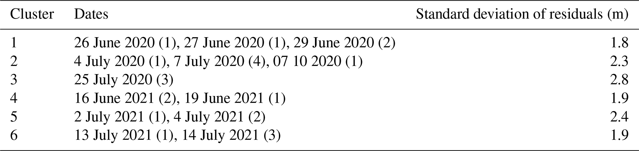
Table A2 Cross-shore change in the upper and lower boundaries estimated from ICESat-2 and the land–water boundaries estimated from Planet at each sampled ICESat-2 location.

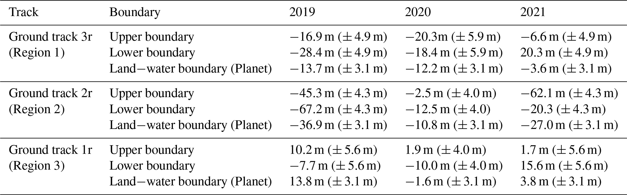
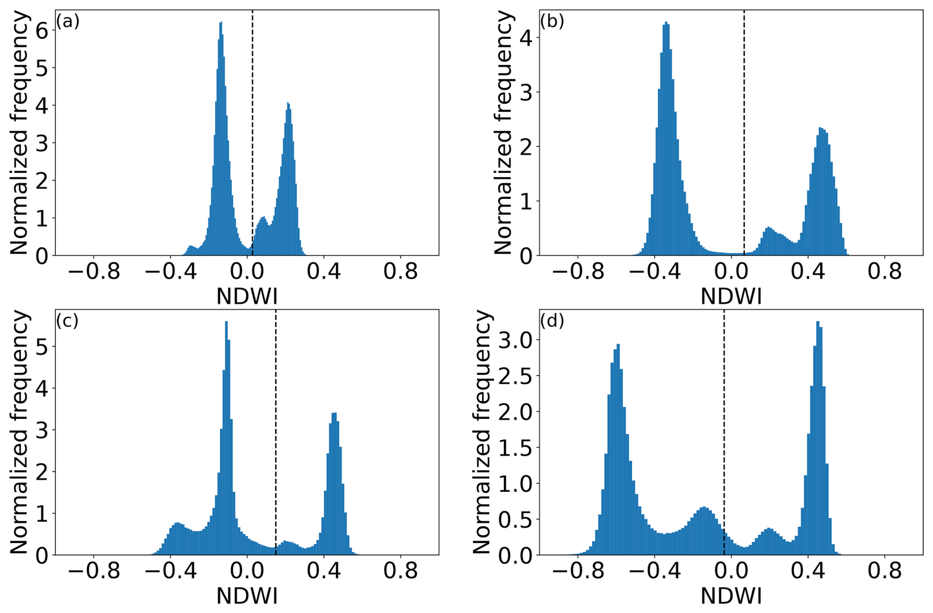
Figure A1 Normalized distribution of scene-wide NDWI values for Planet images collected on (a) 25 June 2019, (b) 25 July 2020, (c) 2 July 2021, and (d) 1 July 2022. The threshold used for identifying the land–water boundary estimated using Otsu’s method is shown as a dashed vertical line.

Figure A2 Illustration of the boundaries and elevation estimates described in Sect. 2.4.

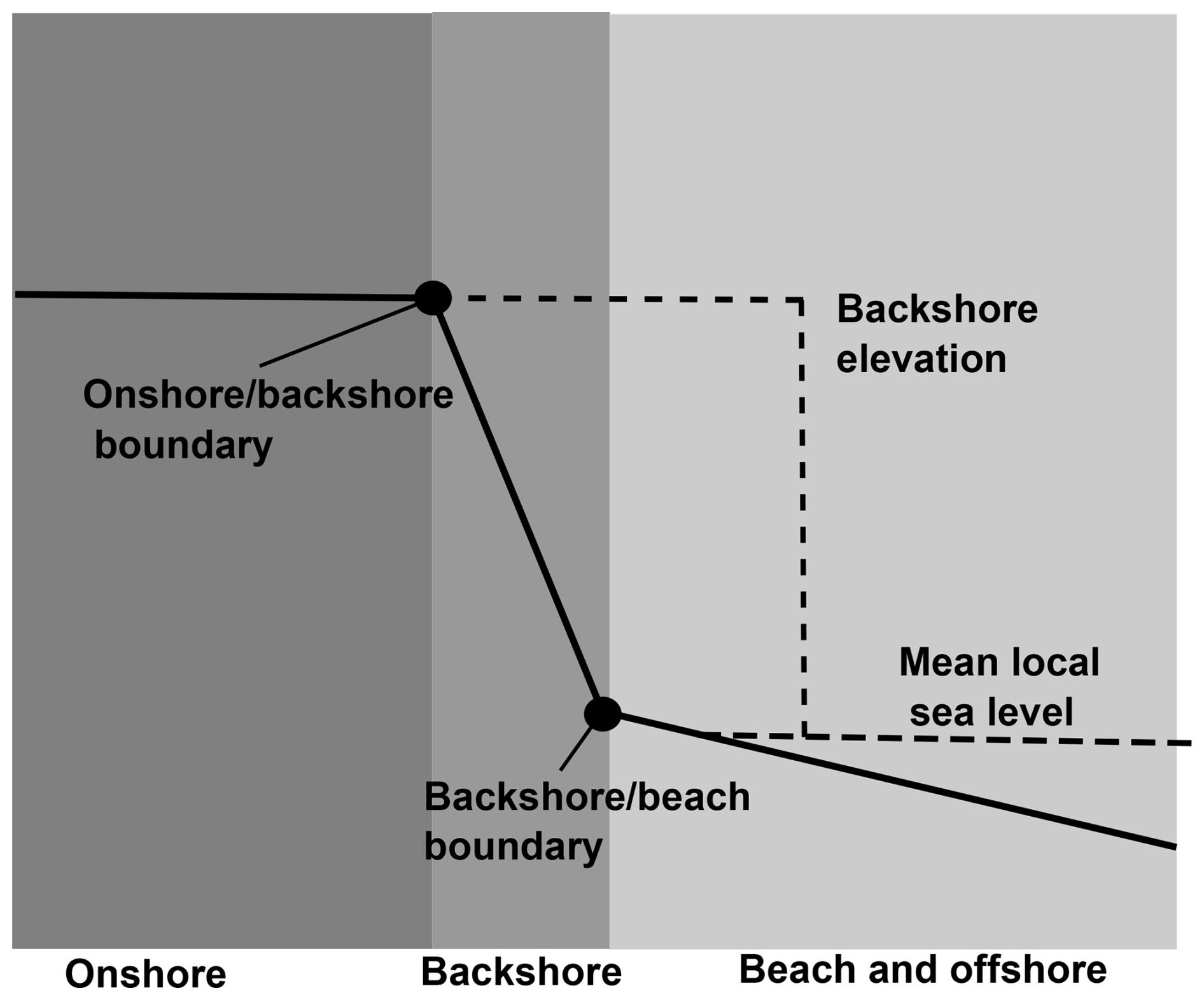
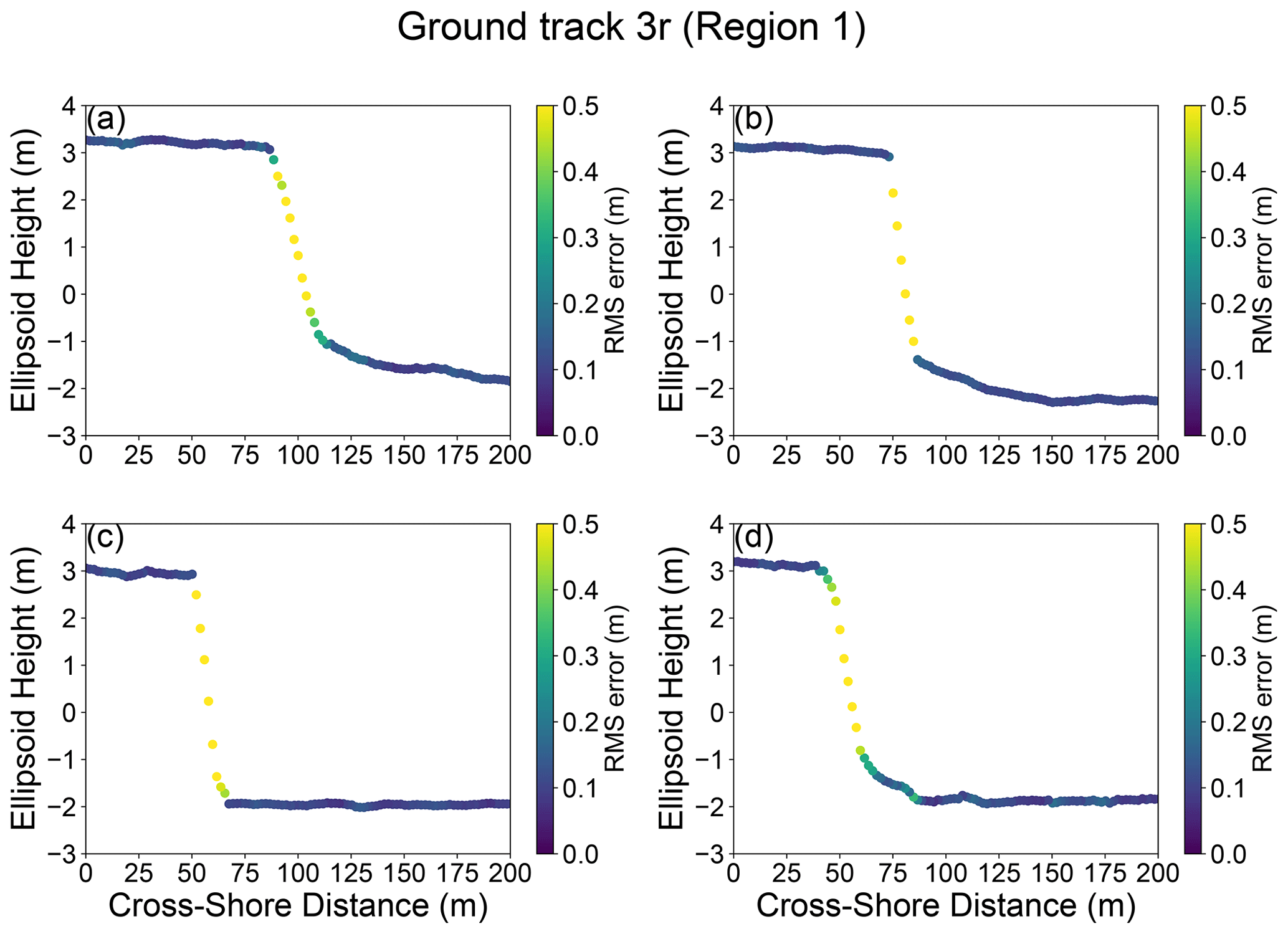
Figure A3 RMS error between our SlideRule-derived elevations and the source ATL03 photon information for ground track 3r on (a) 7 April 2019, (b) 4 January 2020, (c) 2 July 2021, and (d) 31 December 2021.

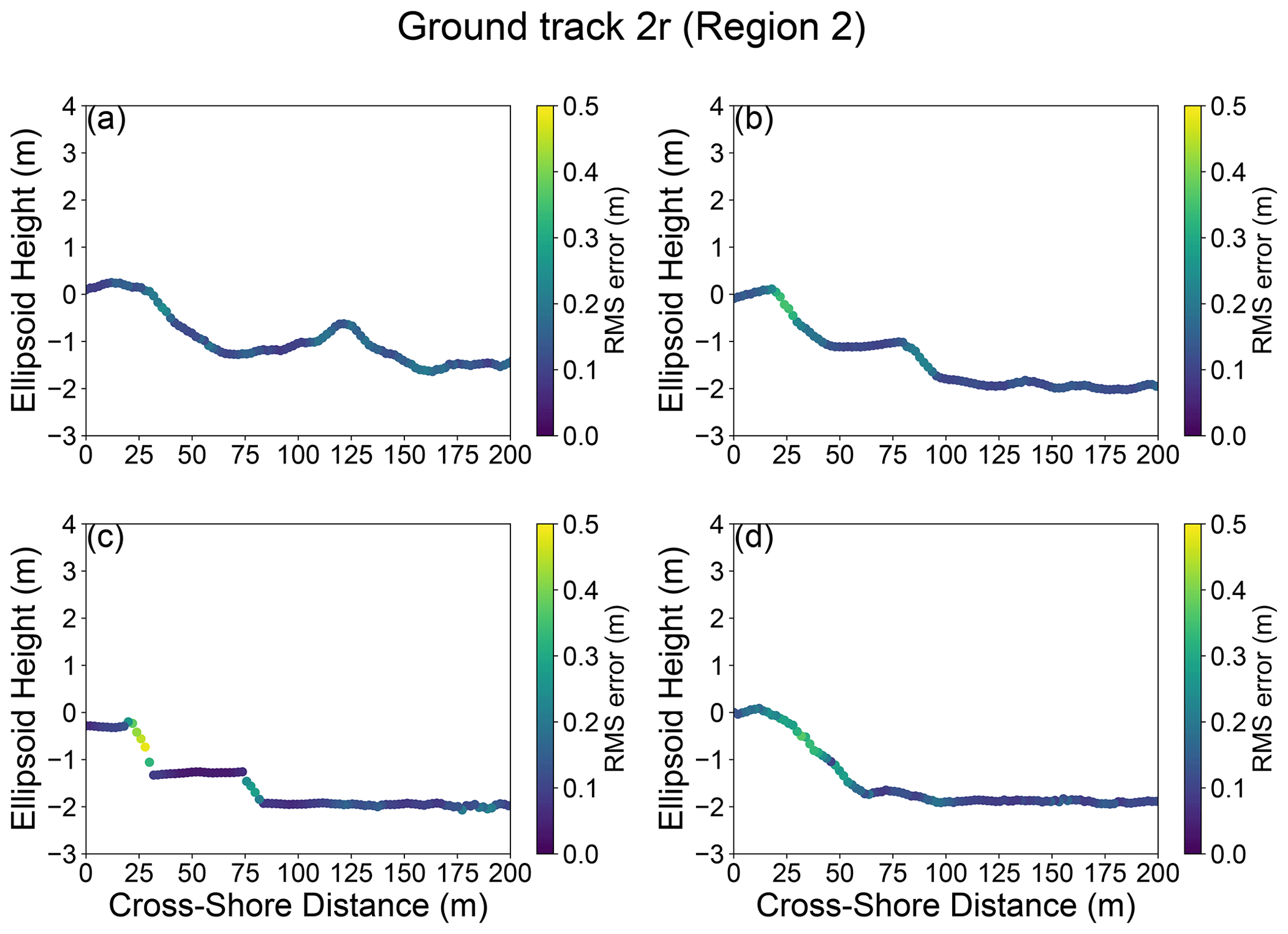
Figure A4 RMS error between our SlideRule-derived elevations and the source ATL03 photon information for ground track 2r on (a) 7 April 2019, (b) 4 January 2020, (c) 2 July 2021, and (d) 31 December 2021.

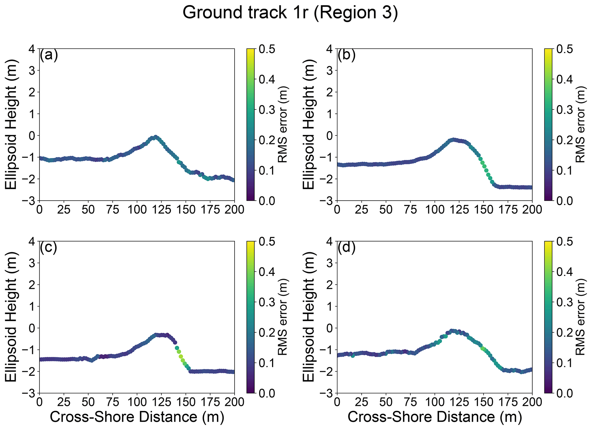
Figure A5 RMS error between our SlideRule-derived elevations and the source ATL03 photon information for ground track 1r on (a) 7 April 2019, (b) 4 January 2020, (c) 2 July 2021, and (d) 31 December 2021.

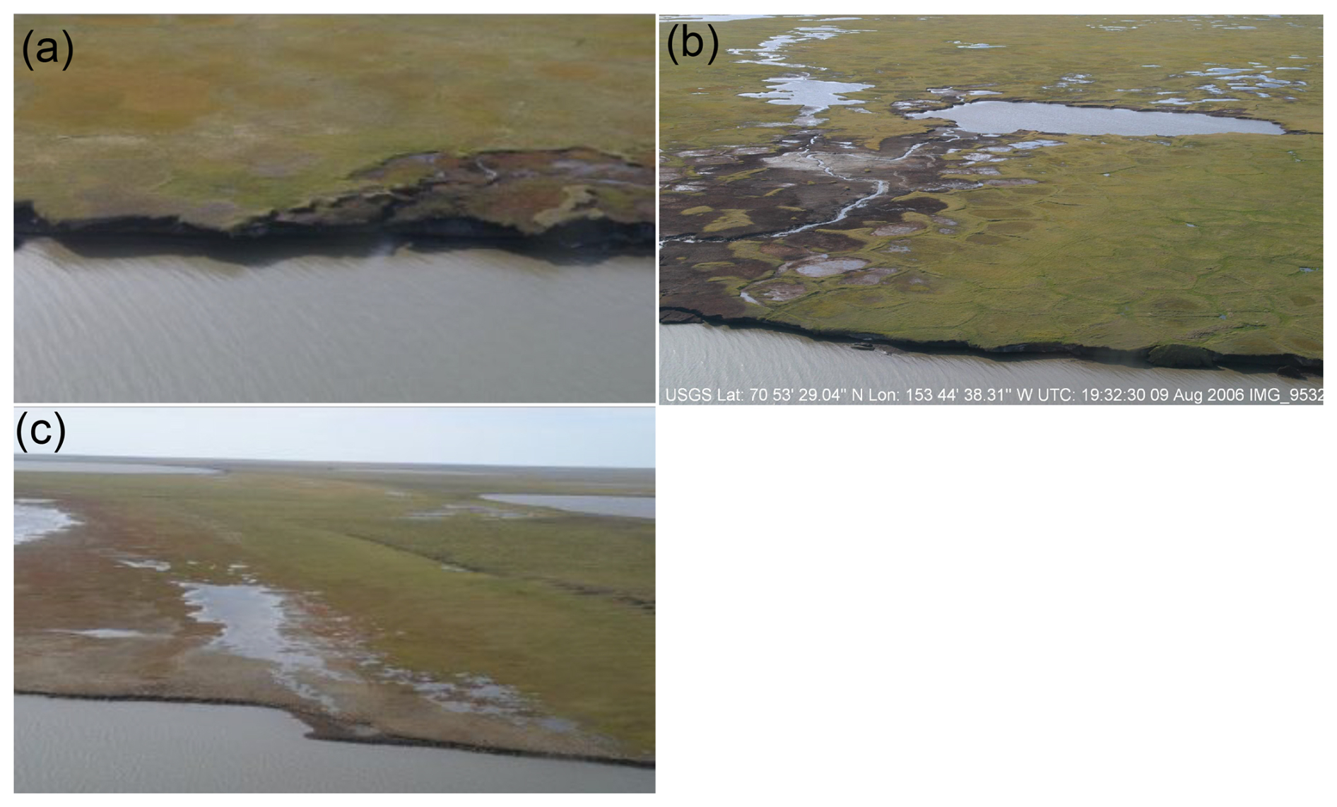
Figure A6 Aerial photography from NOAA ShoreZone in 2007 (Harper and Morris, 2014) captured near the sites of our ICESat-2 ground tracks. (a) A coastal bluff near the sampling site of ground track 3r in Region 1. (b) The small lake sampled by ground track 2r in Region 2 before it drained. (c) The western edge of the large breached thermokarst lake in Region 3 that is crossed by ground track 1r.

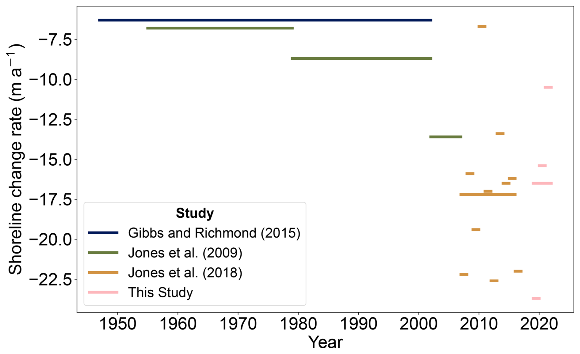
Figure A7 Long- and short-term regional shoreline change rates along the Alaskan Beaufort Sea coast near Drew Point from previous work, along with the 3-year and year-to-year regional rates derived in this work.