the Creative Commons Attribution 4.0 License.
the Creative Commons Attribution 4.0 License.
 | 08 May 2025
The system of atmosphere, land, ice and ocean in the region near the 79N Glacier in northeast Greenland: synthesis and key findings from the Greenland Ice Sheet–Ocean Interaction (GROCE) experiment
Angelika Humbert
Thomas Mölg
Mirko Scheinert
Matthias Braun
Hans Burchard
Francesca Doglioni
Philipp Hochreuther
Martin Horwath
Oliver Huhn
Maria Kappelsberger
Jürgen Kusche
Erik Loebel
Katrina Lutz
Ben Marzeion
Rebecca McPherson
Mahdi Mohammadi-Aragh
Marco Möller
Carolyne Pickler
Markus Reinert
Monika Rhein
Martin Rückamp
Janin Schaffer
Muhammad Shafeeque
Sophie Stolzenberger
Ralph Timmermann
Jenny Turton
Claudia Wekerle
Ole Zeising
The Greenland Ice Sheet has steadily lost mass over the past decades, presently representing the second-largest single contributor to global sea-level rise. In line with the rest of the Greenland Ice Sheet, the glaciers draining the northeast Greenland ice stream have been observed to retreat and thin. Here, we present a comprehensive study of processes affecting and being affected by the mass balance of marine-terminating and peripheral glaciers in northeast (NE) Greenland. Our focus is on the 79N Glacier (79NG), which hosts Greenland’s largest floating ice tongue. We provide new insight into the ice surface melt, the ice mass balance, glacier dynamics, the regional solid Earth response, the ocean-driven basal melt and the consequences of meltwater discharge into the ocean. Our study is based on field observations, remote sensing and simulations with numerical models of different complexity, most of them originating from the Greenland Ice Sheet–Ocean Interaction (GROCE) experiment. We find the overall negative climatic mass balance of 79NG to co-vary with summertime volumes of supraglacial lakes and show that the spatial pattern of the overall negative ice mass balance for NE Greenland is mirrored by the pattern of glacial-isostatic adjustment. We find near-coastal mass losses of both marine-terminating and peripheral glaciers in NE Greenland to be of a similar magnitude in the last decade. In contrast to the neighboring Zachariæ Isstrøm, 79NG – despite experiencing massive thinning of the floating tongue – has resisted an acceleration of ice discharge across the grounding line due to buttressing imposed by lateral friction of the 70 km long ice tongue in the narrow glacial fjord. Observations and models employed in this study are consistent in terms of melt rates occurring below the floating ice tongue. Our results suggest that the multidecadal warming of Atlantic Intermediate Water flowing into the cavity below the ice tongue – supplied by the recirculating branch of the West Spitsbergen Current in Fram Strait – is the main driver of the recent major increase in basal melt rates. We find that the meltwater leaving the cavity toward the ocean at subsurface levels quickly dilutes on the wide shelf. The study concludes by summarizing important estimates of changes to the state of the atmosphere, ice, land and ocean domains.
- Article
(16852 KB) - Full-text XML
- BibTeX
- EndNote


About 25 % of the current global mean sea-level rise is caused by the mass loss of the Greenland Ice Sheet (Milne et al., 2009; Groh et al., 2014; Rietbroek et al., 2016; Horwath et al., 2022), with a substantial increase in the mass-loss rate in recent decades (Shepherd et al., 2012; Khan et al., 2015; WCRP Global Sea Level Budget Group, 2018; Löcher and Kusche, 2021), particularly in very recent years (Mankoff et al., 2021). The resulting rising Greenland freshwater input to the ocean could have significant implications for the North Atlantic thermohaline circulation (Fichefet et al., 2003; Brunnabend et al., 2015; Martin et al., 2022; Lozier, 2023). Decadal circulation changes not only affect regional sea level in the North Atlantic (Chafik et al., 2019) but also alter ocean temperatures, which in turn affect the marine ecosystems (e.g., through Herring recruitment; Toresen et al., 2019).
We first turn to the reasons for the accelerating mass loss of the Greenland Ice Sheet. In their Special Report on the Ocean and Cryosphere in a Changing Climate (SROCC), the Intergovernmental Panel on Climate Change (IPCC) emphasizes that the increasing contribution of the Greenland Ice Sheet to sea-level rise since the 1990s is related to the warming of the surrounding oceans and atmosphere (Meredith et al., 2019). In fact, both the negative trend in surface mass balance and the increased ice discharge into the ocean have contributed to the acceleration of mass loss after 2000 (Pattyn et al., 2018). The strongest increase in mass loss was observed at the margins and lower elevations of the Greenland Ice Sheet, where glaciers are retreating, accompanied by strongly accelerating glacier flow velocity and thinning (Howat et al., 2008; Rignot and Kanagaratnam, 2006; Moon et al., 2012; Joughin et al., 2014; Helm et al., 2014). The contribution of peripheral glaciers (i.e., glaciers dynamically disconnected from the inland ice sheet) compared to the total ice mass loss of Greenland is significant, with estimates ranging from 11 % to 20 % (Bolch et al., 2013; Khan et al., 2022b; Bollen et al., 2022; Kappelsberger et al., 2021), despite the fact that they cover only about 5 % of the total ice area. This underlines the importance of processes between ice, ocean and the atmosphere along the continental margins.
Observations of individual glaciers show that their acceleration and thinning during the recent past is related to a warming of Greenland’s fjord waters (Murray et al., 2010; Straneo and Heimbach, 2013; Straneo et al., 2011; Mayer et al., 2018; Wood et al., 2021), caused by a subsurface inflow of warmer ocean waters from the subtropical Atlantic onto the Greenland continental shelf (as shown in Fig. 1) – hereafter referred to as Atlantic Intermediate Water (AIW) – below the cold and fresh Polar Water. Warmer water at the grounding line and the calving front of marine-terminating glaciers leads to an increased basal and frontal melt (e.g., Straneo and Heimbach, 2013). This may cause the glacier to thin and retreat, resulting in an acceleration of the ice flow upstream. Model studies agree in suggesting the ocean as a very plausible driver of glacier changes (Vieli and Nick, 2011), but the underlying mechanisms are not yet fully understood and are thus not always realistically represented in geophysical models (see Straneo and Cenedese, 2015). Spectacular evidence for ocean changes affecting Greenland glaciers can be found at Jakobshavn Isbræ – Greenland’s largest glacier in terms of ice volume discharge. After a 20‐year phase of continuous, pronounced thinning and retreat, this glacier had started to strongly re‐advance after 2016, supposedly as a consequence of anomalously cold water advected into the local fjord system (Khazendar et al., 2019). Some of the increasing submarine glacier melt over the past decades may, however, actually have been driven by increased subglacial runoff of meltwater from the ice sheet into the glacial fjords, particularly in west Greenland (Slater and Straneo, 2022).
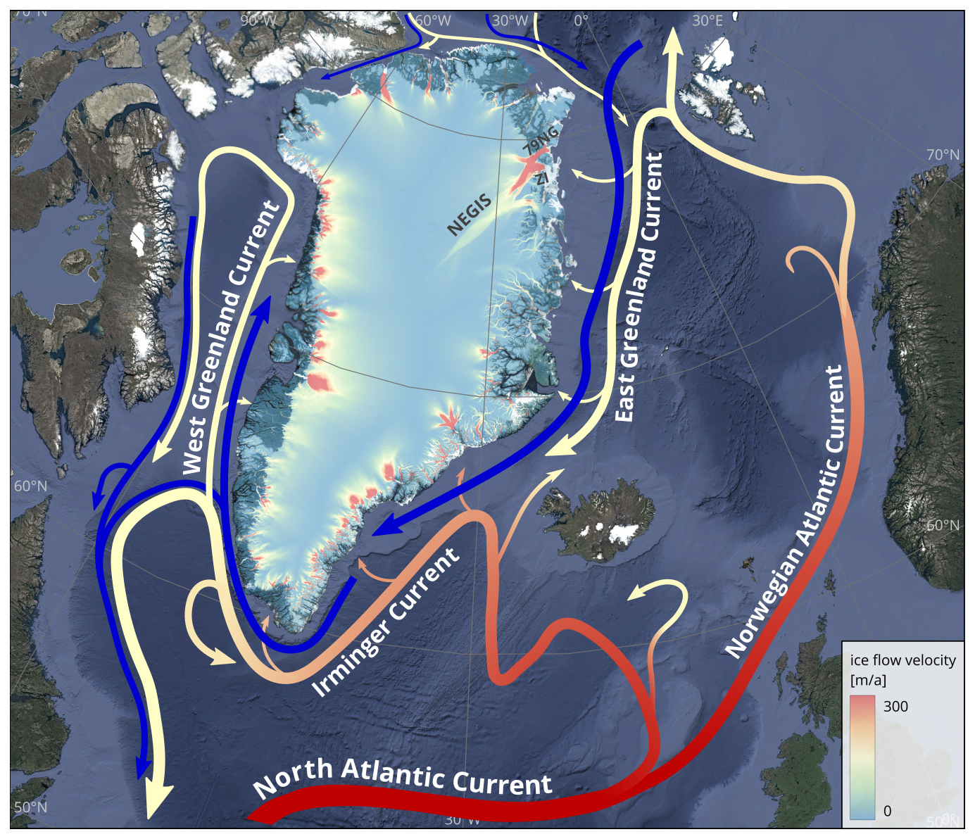
Figure 1The Greenland Ice Sheet with ice-flow velocity (color shaded; Joughin, 2015), the topography of the surrounding ocean and land areas, and the main ocean currents. The red arrows denote warm and saline Atlantic Water (AW) which progressively cools along its flow path, depicted by the color changing from red (warm) to yellow (cooler). When this water subducts below the cold and fresh surface Polar Water (the latter denoted by blue arrows) exported from the Arctic along the continental shelf break of east, south and west Greenland (yellow arrows crossing underneath the blue ones), we refer to it as Atlantic Intermediate Water (AIW). The Northeast Greenland Ice Stream (NEGIS), which separates into 79NG, ZI and Storstrømmen at the ice sheet margin, is seen as a stream of increased ice-flow velocity in NE Greenland. For a zoomed-in representation of the ice sheet–ocean system in NE Greenland, see Fig. 3.
Regarding the importance of mass loss by surface melt relative to that by increased ice discharge, Mouginot et al. (2019) found that more than 60 % of the Greenland Ice Sheet mass loss has been due to ice discharge over the past 50 years. However, in recent years, the surface mass balance has played an increasingly important role, adding the atmosphere as a critical player (Meredith et al., 2019), interlinked by complex processes with the glacier surface (Mölg and Kaser, 2011). A temporary acceleration of ice mass loss in 2012 was linked to atmosphere‐induced surface melt in southwest Greenland (Bevis et al., 2019), followed by another acceleration in 2019 (Sasgen et al., 2020; Khan et al., 2022a), and air temperatures on the central Greenland Ice Sheet in the first decade of this century appear to have been the highest throughout the past millennium (Hörhold et al., 2023). For floating ice tongue glaciers, the varying subsurface discharge of glacial meltwater forms another source of variability that partly originates from surface melt and enters the ocean at the grounding line and at the sloping ice base downstream, modulating the melt processes in the cavity beneath the floating ice tongue (Rignot et al., 2010; Motyka et al., 2011; Enderlin and Howat, 2013; see schematic in Fig. 2). For Antarctic ice shelves, the impact of subglacial discharge on basal melt rates appears to be less important (Nakayama et al., 2021).
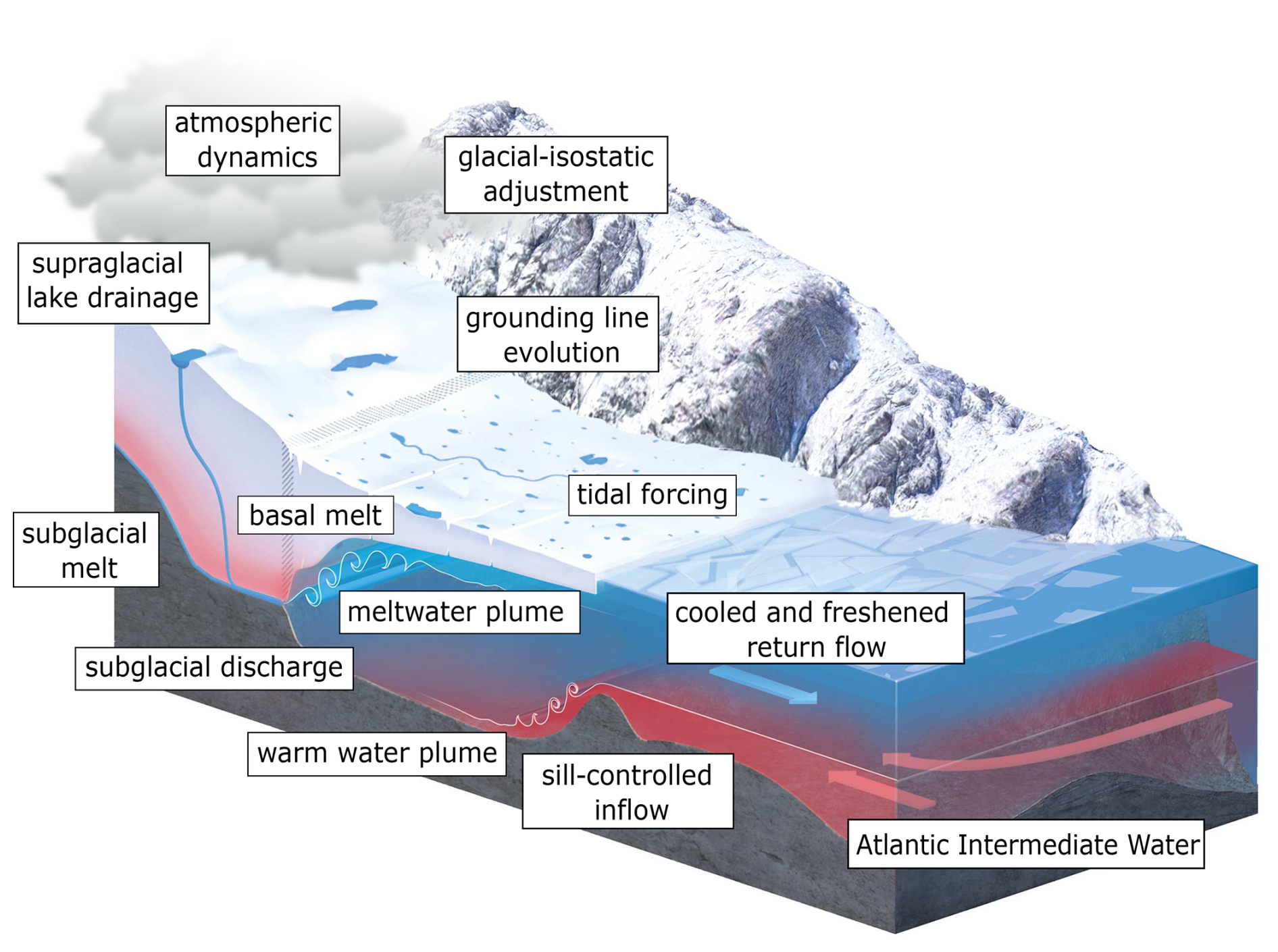
Figure 2Graphic depiction of the NEGIS–79NG ice sheet–ocean system showing the ocean, atmosphere, land and glacier processes involved in ocean–glacier interactions, inspired by our results regarding the mass balance of 79NG. The floating ice tongue is a prominent characteristic of 79NG, affecting glacier dynamics and ocean-driven glacier melt.
Thus far, ice mass loss has been observed in all regions around the Greenland Ice Sheet margin, with strong contributions from marine-terminating outlet glaciers (Rignot et al., 2010; Helm et al., 2014; The IMBIE team, 2018; Mouginot et al., 2019). The retreat of these glaciers coincides with the warming of AIW (e.g., Straneo and Heimbach, 2013; Wood et al., 2021). In recent years, the warming of the North Atlantic has also penetrated into the Nordic Seas and the Arctic Ocean (Beszczynska-Möller et al., 2012; McPherson et al., 2023b), amounting to almost 1 °C warming in the West Spitsbergen Current (WSC) between 1997 and 2018.
The collapse of the floating ice tongue of Zachariæ Isstrøm (hereafter ZI) in northeast (NE) Greenland is one of the most prominent examples of rapid glacier retreat (Mouginot et al., 2015). Currently, the largest remaining floating ice tongue by area in Greenland is that of the 79N Glacier (hereafter 79NG), which is 70 km long and located just north of ZI. Studies based on remote sensing data report melting and thinning of the 79NG glacier tongue (Kjeldsen et al., 2015; Mouginot et al., 2015; Khan et al., 2014), with estimates of up to 30 % total ice thickness loss over the past 20 years (Mayer et al., 2018). This thinning appears to be caused by a mass imbalance due to increased melt along the ice tongue base (Wilson et al., 2017; Mayer et al., 2018) caused by ocean heat fluxes. Based on water mass analyses, Schaffer et al. (2017) were able to demonstrate the existence of a pathway of warm AIW recirculation in Fram Strait across the NE Greenland continental shelf towards 79NG. They also showed that the AIW on the continental shelf close to 79NG has warmed by 0.5 °C over the past few decades, driven by the advection of the warming Atlantic Water in the WSC across Fram Strait which penetrates onto the continental shelf (McPherson et al., 2023b). In contrast, the reason for the collapse of the floating ice tongue of ZI is less clear (Mouginot et al., 2015).
The need to assess and understand the changing ice sheet–ocean system of NE Greenland was the starting point of the Greenland Ice Sheet–Ocean Interaction (GROCE) project. GROCE was funded by the German Ministry of Education and Research (BMBF). It consists of scientists from several universities and research centers contributing their expertise in observations, remote sensing, and modeling of ocean and glacier dynamics, as well as processes in the atmosphere and the lithosphere on a wide range of scales. The objective of GROCE is to understand critical mechanisms and their interactions in controlling the NE Greenland Ice Stream (NEGIS) ocean–glacier interaction, with a focus on 79NG. 79NG itself has a floating ice tongue of approximately 70 km length and 20 km width, extending to a 30 km wide calving front. It covers the entire fjord with a thicknesses of 100 m at the calving front to maximum values exceeding 600 m at the grounding line. Below the ice tongue, there is a cavity up to 900 m deep. The glacier bed topography reconstructed from BedMachine Greenland (Morlighem et al., 2017) reveals a grounding-line depth of 600 m in 1996 at the center of 79NG and lower values toward the margin. These depths were confirmed by active seismic measurements by Mayer et al. (2000) from 1998.
Topically connected studies of local processes and observational programs in the ocean, on 79NG and at adjacent land areas of NE Greenland have formed the basis of our research. Figure 2 highlights the variety of processes relevant to the coupled system. The consortium has examined atmospheric processes affecting the surface melt and the drainage of meltwater from supraglacial lakes to the glacier base. We have also examined the effects of the drained surface meltwater entering the cavity across the grounding line (subglacial discharge) and of the warm AIW entering the cavity from the NE Greenland continental shelf on the meltwater plume dynamics and basal melt in the cavity and on frontal ablation (Fig. 2). Furthermore, the impact of tides and ice shelf retreat on the ice sheet velocity field upstream and the role of the distribution of meltwater outflow for the regional ocean circulation have also been research topics. And lastly, we have investigated the impact of the glacial-isostatic adjustment on the complex solid Earth–ice–ocean system, particularly in the marginal zones of the NEGIS. The expeditions GRIFF (Greenland ice sheet/ocean interaction and Fram Strait fluxes; PS100) and GRISO (Greenland ice sheet/ocean interaction; PS109) conducted aboard the German research icebreaker RV Polarstern in 2016 and 2017 lay the foundations for not only much of the oceanographic research but also glaciological and geodetic work (Kanzow, 2017, 2018), while the oceanographic moorings deployed in 2017 were recovered aboard HDMS Triton in 2021 (McPherson et al., 2023a).
As pointed out in Sect. 1, there are a variety of studies that provide ice mass balance estimates for Greenland. The motivation of this article is to bring together the many individual, in-depth studies of GROCE, based on both already published research and new data. From this we derive the main aim, which is to provide (i) a process-based, holistic understanding of the ice mass balance of the NEGIS–79NG system and (ii) a quantitative assessment of the involved mass balance components. Our approach incorporates a synthesis of processes from the atmosphere to ice, to ocean and to the lithosphere. In Sect. 3, we give a summary of the datasets and employed methods. Section 4 presents the results starting from the atmosphere and moving on via the cryosphere and land domains to ocean processes. We also explore the first causal links between these spheres in that chapter. And finally, Sect. 5 attempts to bring the results together into a consistent understanding of the NEGIS–79NG mass balance and to discuss aspects in a general ice sheet (Greenland and Antarctica) context.
In this chapter, we briefly introduce the data and methods applied. Since datasets and methods have been previously published in peer-reviewed papers to a large extent, we keep the description of each element short and refer to the literature for more detailed information. Figures 3 and 4 summarize the datasets and their geographical origins in the 79NG area.
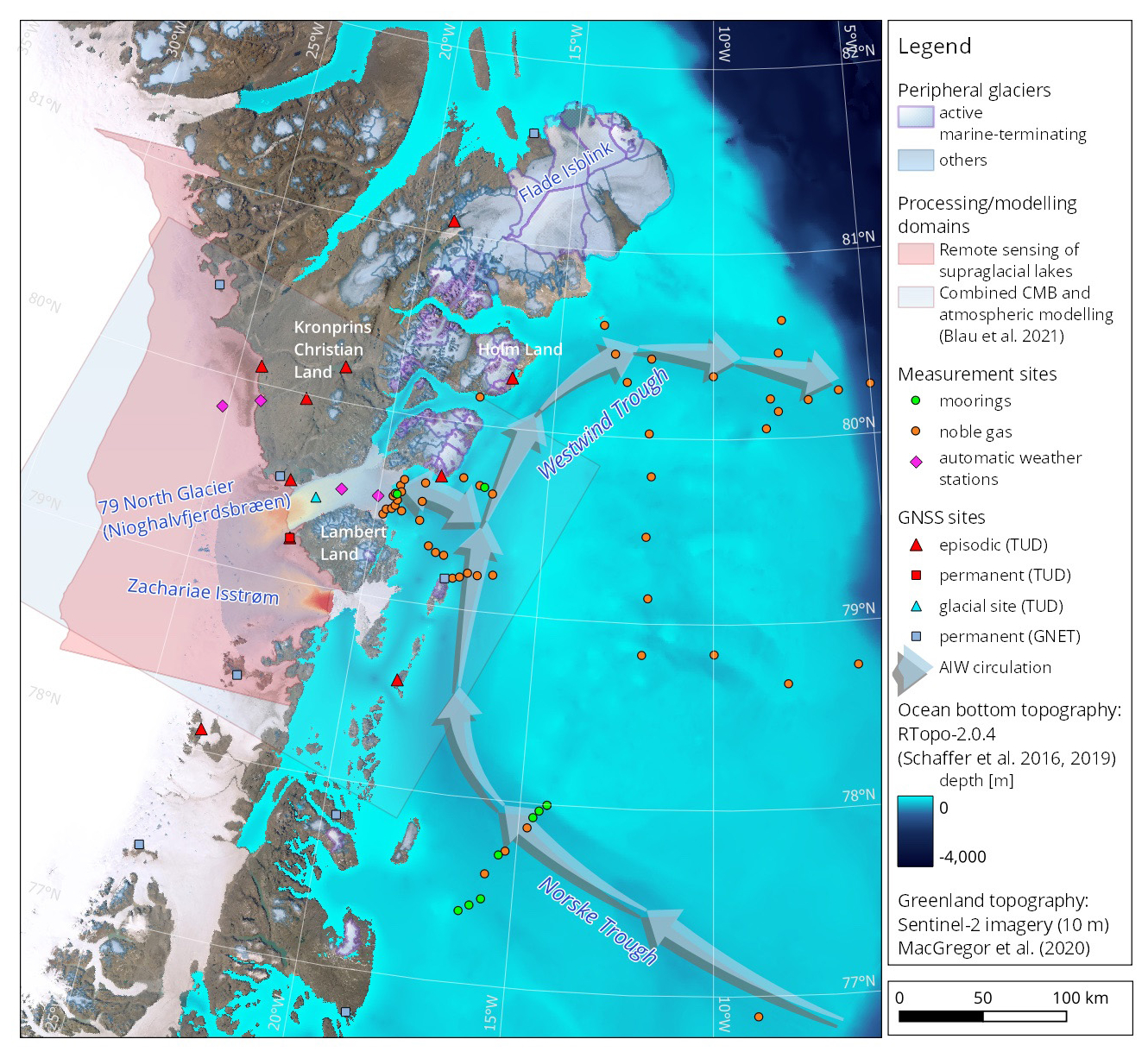
Figure 3Geographic overview over the near-coastal NEGIS (79NG and ZI) area out to the continental shelf break of NE Greenland. Also shown are the geographic locations of in situ data and remote sensing datasets used in and produced by the GROCE project in the ocean on the continental shelf, on the floating ice tongue of 79NG, on the grounded ice and on the solid Earth. Gray arrows denote the pathway of the AIW circulation in the ocean along the Norske Trough–Westwind Trough system. TUD: TUD Technical University of Dresden. GNET: Greenland GNSS (global navigation satellite system) Network.
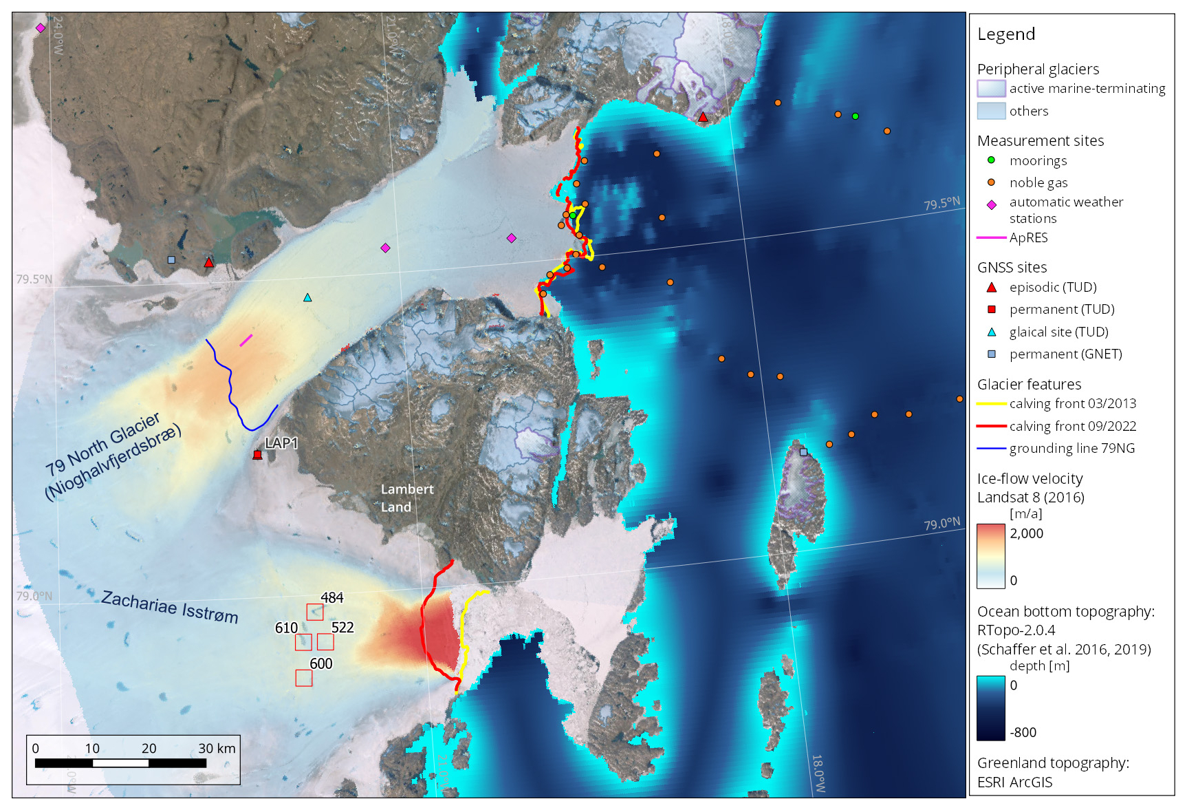
Figure 4Detailed map focusing on 79NG and ZI and the inner continental shelf (zoomed-in representation of the map shown in Fig. 3). The ice-flow velocities are based on Landsat 8 imagery recorded in 2016 (processing according to Rosenau et al., 2015). Calving fronts were inferred from Landsat 8 and Landsat 9 imagery (see Sect. 3.6). Annotated red rectangles denote the location of supraglacial lakes where in situ measurements of water depths were taken. ApRES: autonomous phase-sensitive radar.
3.1 Regional atmospheric and climatic mass balance modeling
The basis for inferring the climatic mass balance is the polar version of the Weather and Research Forecasting (WRF) model (Hines et al., 2011). WRF is a non-hydrostatic numerical atmospheric model that has been extensively used and tested at many scales and in various regions (Powers et al., 2017). Our applications (version 3.9.1.1) concerned (1) a case study to examine processes of wintertime melt over ∼ 20 d in 2014 (Turton et al., 2019) and (2) the generation of a highly spatially (1 km) and temporally (up to 1 h) resolved atmospheric modeling dataset over 79NG and the NE Greenland Ice Stream for 2014–2018, called NEGIS_WRF (Turton et al., 2020).
The output from this simulation serves as forcing for the COupled Snowpack and Ice surface energy and mass balance model in PYthon (COSIPY) (Sauter et al., 2020). This model calculates the mass balance at the surface and near the surface (water storage and melting/refreezing in the snow), the sum of which is known as “climatic” mass balance (CMB). The COSIPY–NEGIS_WRF setup (Fig. 5) delivered multiannual fields of the CMB every 1 km for the 79° N region (Blau et al., 2021), which in the GROCE framework represents the atmosphere–cryosphere interface.
3.2 Meteorological data
Hourly resolution records from automated weather stations (AWSs) were utilized to examine the atmospheric conditions in the region of 79NG and evaluate the modeling above (purple diamonds in Fig. 3). AWS 9602 and AWS 9604, from an earlier field program, provided data for the middle to late 1990s on the floating shelf (Højmark Thomsen et al., 1997), while two AWSs from the Programme for Monitoring of the Greenland Ice Sheet (PROMICE) network delivered data since the late 2000s for Kronprins Christian Land (KPC). Near-surface air temperature, relative humidity, wind speed and direction, air pressure, shortwave radiation, longwave radiation, cloud cover, and skin temperature were among the variables considered from AWSs.
The European Centre for Medium-Range Weather Forecasts (ECMWF) ERA-Interim reanalysis dataset (Dee et al., 2011) spanning 1979 to 2017 was used alongside the AWS observations to compensate for their sparse and intermittent observing period.
3.3 Dataset of evolving supraglacial lake volumes
To quantify the amount of meltwater gathering on the glacier surface and subsequently draining to the glacier bed (see Fig. 2) or running off through surface channels into the ocean, we developed a method to identify the dynamic boundaries of supraglacial lakes (Hochreuther et al., 2021) which we apply to estimate lake areas. This method uses Sentinel-2 multispectral data to segment the lakes on a daily basis from 2016 to 2022 and a thresholding technique, taking advantage of the prominence of lakes in the blue and red spectral bands. We extend our previous research using a widely accepted supraglacial lake depth algorithm to provide a rough volume estimate of the lakes. Originally proposed by Philpot (1989) and further developed by Sneed and Hamilton (2007), this method employs the principles of radiative transfer theory to determine the lake depth from an optical image. A summary of this lake depth algorithm is also given in Lutz et al. (2024a). In order to reduce the noise in the lake volume time series, the estimates are exclusively based on cloud-free conditions, which are subsequently interpolated onto a regular time grid. Finally, for smoothing purposes, a Savitzky–Golay filter is applied to the lake volume time series. The methodology is applied to all supraglacial lakes contained in the area just upstream of the grounding line of the 79NG area (pink-shaded area in Fig. 3).
3.4 Tidal response of glaciers
Observed tidal motion of the floating tongue of 79NG (Fig. 4) is used as a forcing for the subglacial hydrology model CUAS (Beyer et al., 2018) and viscoelastic simulations using COMice-ve (Christmann et al., 2021; Fig. 5). The CUAS setup uses an updated version of the BedMachine topography (Morlighem et al., 2017) including the Alfred-Wegener-Institut (AWI) flight lines in the 79NG region acquired within the GROCE project (Christmann et al., 2021) and parameters as used in Beyer et al. (2018). CUAS simulations are conducted at a resolution of 300 m in the vicinity of the grounding line of 79NG and of 1200 m over the entire NEGIS. We consider water input by basal melt in the grounded area arising from geothermal flux and basal friction taken from Aschwanden et al. (2016). The tidal forcing (Fig. 2) is expected to modulate the effective pressure in the CUAS simulation (mostly at the grounding line), which is fed into COMice-ve to estimate the consequences on the ice flow.
3.5 Determination of frontal positions and ice-flow velocity fields by an advanced deep neural network
The processing combines data of the remote sensing satellites Landsat 8 and Landsat 9. The inference of ice-flow velocity fields is based on the feature tracking method as implemented and described by Rosenau et al. (2015). For the inference of frontal positions, a deep neural network was implemented (Loebel et al., 2022). A thorough assessment of the achievable accuracy using diverse datasets was carried out, supplementing the single-band inputs with multispectral data, topography data and textural information. The resulting feature importance shows a clear benefit utilizing multispectral bands (Loebel et al., 2022). With their inclusion, frontal-position predictions are generally more accurate than using conventional single-band inputs only (Loebel et al., 2022). On the contrary, the inclusion of both topographic and textural information cannot be favored since it may cause model overfitting. As a result, between 2013 and 2021 we could infer about 150 flow velocity fields per year for 79NG and ZI as well as about 40 to 60 frontal positions per year for each glacier (Fig. 4). It could be shown that our method allows us to achieve a considerably higher extraction rate than other (automation) methods; thus it was possible to infer time series of frontal positions resolving long-term, seasonal and subseasonal variations (Loebel et al., 2024). Additionally, a rectilinear-box method was implemented which allows us to discriminate the proportionate glacier-covered area from the uncovered area (cf. Fig. 8). In this way the temporal variations in the frontal positions could be visualized in a much better way, also demonstrating the higher temporal resolution compared to other available datasets (Loebel et al., 2024).
3.6 Sensitivity studies of the 79NG ice discharge
To assess the upper-end effect of the ice discharge of 79NG on sea-level change, we conduct a series of model simulations of three scenarios by sequential removal of increasingly larger frontal parts of the 79NG floating tongue up to a full collapse (i.e., the removal of the entire tongue), following Humbert et al. (2023). The simulations using the ice sheet model ISSM (Larour et al., 2012) and the initial state are based on a joint inversion for the basal friction coefficient on grounded ice and the ice hardness in floating ice. The friction law is of a non-linear Budd type (Budd et al., 1984). The geometry is based on BedMachine v4 (Morlighem et al., 2017). We define three future states: (1) calv-iceberg, assuming a calving of a larger part at the eastern ice front; (2) calv-fjord, with a retreat up to a bottleneck within the fjord leaving a 45 km long tongue; and (3) collapse, with the total collapse of the floating tongue. We analyze the 3D simulations as cross-sections in the along-flow direction and across the grounding line. The variables discussed here are surface velocity, ice flux across the grounding line and buttressing.
3.7 An approach to studying the mass balance of the Greenland Ice Sheet
We combined two major techniques for observing ice sheet mass balance (Kappelsberger et al., 2021). Firstly, we analyzed results from GRACE and GRACE-FO satellite gravimetry, which is directly sensitive to mass changes, using the monthly solutions inferred by Bettadpur (2018) and by Kvas et al. (2019) given in a spherical harmonic representation. We applied the method of tailored sensitivity kernels (Groh and Horwath, 2021) which integrates the concepts of region definition, filtering according to known noise characteristics and minimization of leakage effects. The effect of glacial-isostatic adjustment (GIA) is corrected for by subtracting the mass effect predicted by the respective GIA model (see Sect. 4.7 and 4.8).
Secondly, satellite altimetry measures ice surface elevation and allows us to infer surface elevation change (SEC). We used CryoSat-2 data pre-processed with regard to the acquisition mode (LRM, low-resolution mode; SARIn, synthetic aperture radar interferometric) according to Krieger et al. (2020) and Helm et al. (2014), respectively. We conducted a repeat altimetry analysis (Kappelsberger et al., 2021) over the Greenland Ice Sheet and the peripheral Flade Isblink Ice Cap (Fig. 3). This analysis provides SEC rates in a 1.5 km × 1.5 km grid, determined by least-squares adjustment together with further parameters accounting for local topography, seasonal variation and the time-variable radar penetration effect. For the peripheral glaciers, except the Flade Isblink Ice Cap (FIIC), the SEC product published by Simonsen and Sørensen (2017) was used. The effect of GIA bedrock uplift was corrected for taking predictions by respective GIA models into account (see Sect. 4.7 and 4.8). Volume changes were converted to mass changes by employing a density model based on both the firn densification model IMAU-FDM (Ligtenberg et al., 2018) and on a velocity-based criterion for assuming dynamic ice mass imbalances.
Finally, the results (including uncertainty ranges) from the two complementary techniques were combined into a consistent parameter estimation approach (Kappelsberger et al., 2021). The resulting grid of mass change rates (given over the period of 2010 to 2017; Kappelsberger et al., 2020) maintains the high spatial resolution of satellite altimetry and, at the same time, adheres to the mass change constraints provided by satellite gravimetry.
3.8 Response of the solid Earth to mass changes
The bedrock displacement (Fig. 2) was determined by in situ measurements using geodetic GNSS recordings in the ice-free regions of NE Greenland. We carried out campaign-style measurements at 10 sites between 78 and 81° N in 2008/09, 2016 and 2017 (Fig. 3). Additionally, data of the continuously recording GNET stations (Khan et al., 2016) were included. The GNSS data were analyzed using the differential processing approach incorporating the required precise data and correction models (Kappelsberger et al., 2021). The solution refers to the GNSS-only realization IGS14 (Rebischung et al., 2016) of the International Terrestrial Reference System, with CM (center of mass of the Earth system) adopted as the origin. Finally, 3D linear velocities were inferred with uncertainties of 1 mm a−1 for the horizontal components and 1.5 mm a−1 for the vertical component (Sect. 4.8).
3.9 An approach to modeling peripheral glaciers
We used the Open Global Glacier Model (OGGM; Fig. 5) (Maussion et al., 2019) to simulate the Flade Isblink Ice Cap (FIIC) in the vicinity of 79NG in NE Greenland (Fig. 3). We subdivided FIIC based on the ArcticDEM data (Porter et al., 2018) into 299 individual glacier basins (Fig. 12a). Using different ice velocity data (Gardner et al., 2022; Joughin, 2015), six out of nine marine-terminating basins were detected as active calving basins (Recinos et al., 2021). The frontal ablation of marine-terminating glaciers was computed using a dynamic parameterization based on the calving law formulated by Oerlemans and Nick (2005) and applied at a large scale by Huss and Hock (2015). However, we refined this approach by incorporating mass conservation principles to estimate the thickness of the calving front, which was determined by reconciling the amount of ice delivered to the terminus by OGGM with the amount of ice calved (Recinos et al., 2019).
We also used the NEGIS_WRF atmospheric data (Sect. 3.1) from 2014 to 2018 at 5 km resolution for one of the OGGM simulations. Additionally, the datasets ERA5 (∼ 30 km) and CRU (∼ 50 km; Climatic Research Unit) (Harris et al., 2020) were employed in order to analyze the sensitivity of glacier processes to input data resolution. Similarly, gridded rates of ice mass change based on the combination of satellite gravimetry (GRACE) and altimetry (CryoSat-2) at a fine resolution of 1.5 km × 1.5 km (Kappelsberger et al., 2021) (Sect. 3.7) were used to calibrate OGGM for the glacier basins outlines of FIIC (Fig. 12c). Geodetic mass balance data (Hugonnet et al., 2021) were used for the rest of the peripheral glaciers in NE Greenland. Finally, future glacier mass loss and freshwater runoff contributions were projected for all peripheral glaciers in NE Greenland using CMIP6 (10 general circulation models (GCMs) and 4 emission scenarios) climate forcing and OGGM. The selected GCMs have been employed in several previous studies for similar projections (Rounce et al., 2023; Zhao et al., 2023; Edwards et al., 2021; Malles et al., 2023). As in the studies mentioned above, the selected GCMs were bias-corrected using the delta method (Maraun, 2016), which involved employing relatively high-resolution gridded observations as the reference climatology (Copernicus Climate Change Service, 2019) and applying only anomalies from the GCMs relative to a pre-determined reference period (1981–2019). Ice discharge from FIIC basins 2 and 3 (Fig. 12b) forms a continuous ice shelf that extends towards the northwest. We determined the grounding-line locations of these basins and analyzed their variability with time (Möller et al., 2022).
3.10 Observations of Atlantic Intermediate Water flow toward 79NG and inferred basal melt rates
Over the last decade, dedicated oceanographic measurements have been carried out on the continental shelf of NE Greenland relevant to the ocean impact on 79NG. During the RV Polarstern expedition PS85 in 2014, an array of seven moorings measuring temperature and velocity were deployed across Norske Trough (Fig. 3), with the inflow pathway of warm AIW toward 79NG (Schaffer et al., 2017). The array was recovered in summer 2016 during the expedition PS100 and laid the foundation of the study of AIW circulation and connection from the shelf edge to the mid-shelf (Münchow et al., 2020). The expedition PS100 was also used to deploy moorings (measuring velocity, temperature and salinity) in the direct vicinity of 79NG for the first time, informed by hydrographic and bathymetric surveys (Schaffer et al., 2020) which revealed a complex system of sills and channels guiding the flow of AIW into the cavity under the floating ice tongue of 79NG (Fig. 4). The moorings were recovered and partly redeployed in 2017 during the RV Polarstern expedition PS109, with a final recovery close to 79NG in summer 2021 aboard the Danish coastguard vessel HDMS Triton. The data were used to study pathways; volume and heat transport; and underlying dynamics associated with the AIW flow toward 79NG, including estimates of basal melt rates (Schaffer et al., 2020; von Albedyll et al., 2021; McPherson et al., 2023b, 2024). The bathymetry data mainly collected during the expedition PS100 were used to update a global bathymetry grid (RTopo-2.0.4; Schaffer et al., 2019a), which then fed back into the Finite-Element/volumE Sea ice-Ocean Model (FESOM) ocean–sea ice model configuration developed in the project (Sect. 3.13).
3.11 Basal melt of 79NG’s floating tongue from in situ radar observations
Basal melt rates are measured using an autonomous phase-sensitive radar (ApRES) instrument that continuously acquired data from August 2016 to January 2020. From August 2016 to July 2018 the instrument moved with the glacier over a distance of about 2.5 km, making this a Lagrangian observation (magenta line in Fig. 4). In July 2018 the instrument was relocated to the original start location in August 2016 such that the trajectory was occupied twice so that temporal changes in basal melt might be distinguishable from spatial ones. The instrument was deployed about 6 km downstream of the grounding line. We basically observe the change in ice thickness over time by tracking the basal reflection and assessing the influence of stretching by deformation. More details on the method are given in Zeising et al. (2024a). As the base of the floating tongue is rough, side reflections influence our ability to detect the basal melt rate in the nadir direction.
3.12 Quantification of the basal meltwater from noble gas data
To identify and to quantify the distribution of basal meltwater on the NE Greenland shelf, we use helium (He) and neon (Ne) observations. They have been sampled during the expeditions PS100 (in 2016) and PS109 (in 2017) on the NE Greenland shelf. On the RV Maria S. Merian expedition MSM85 (2019), hydrographic and tracer sections across the East Greenland Current from the Irminger Sea to 79NG were taken to put the results from 79NG in a broader perspective (Mertens et al., 2020). The calculation of the basal meltwater follows the approach described in detail in Rhein et al. (2018) and Huhn et al. (2021a). Atmospheric air with a constant composition of the noble gases He and Ne is trapped in the ice matrix during the formation of meteoric ice. When the ice melts at depth or at the ice base inside a glacier cavity, these gases are completely dissolved in the water, due to the enhanced hydrostatic pressure. This leads to an excess of DHe = 1280 % and DNe = 890 % in pure basal meltwater (Loose and Jenkins, 2014); the D stands for the gas excess over the air–water solubility equilibrium. In contrast, melt at the glacier surface would equilibrate quickly with the atmosphere and does not show a noble gas excess in ocean water. This is also true for freshwater discharged into the cavity across the grounding line originating from supraglacial melt (Huhn et al., 2021a).
3.13 Multiscale approach to comprehensively simulating cavity circulation, basal melt and the spreading of basal meltwater
We take a multiscale approach in simulating the basal melt associated with 79NG (Fig. 5). Idealized (i) 2D and (ii) 3D approaches are taken to understand the governing processes in the glacier cavity driving the basal melt (Fig. 2) and influencing the melt rate distribution. (iii) A plume model assesses the effects of key factors influencing plume dynamics, such as the roughness at the base of the ice and basal channels. (iv) A high-resolution configuration of the Finite-volumE Sea ice-Ocean Model (FESOM2.1) with a realistic representation of the cavity geometry of 79NG is used to study changes in the melt rates in response to a hierarchy of driving factors (most importantly, AIW temperature on the NE Greenland continental shelf and subglacial discharge into the cavity). (v) Another FESOM setup with increased mesh resolution around Greenland is then used to study the impact of glacial meltwater from the ice sheet on circulation and hydrography in the Nordic Seas and the subpolar North Atlantic. In the following the different models are introduced.
-
2D fjord model. To resolve subglacial-meltwater plumes (Fig. 2), which are buoyant turbulent gravity currents underneath ice shelves modified by subglacial discharge, basal meltwater and the entrainment of warm AIW, we constructed an idealized 2D model of the 79NG fjord (Reinert et al., 2023) using the coastal ocean model GETM (Burchard and Bolding, 2022; Fig. 5). As typical meltwater plume thicknesses are on the order of 10 m, a very high vertical resolution is needed. Here we used adaptive vertical coordinates (Hofmeister et al., 2010) with high resolution in the vertical direction and along the fjord axis. The vertical coordinates adapt to the stratification in a way that coordinate layers accumulate at locations of enhanced vertical stratification (see applications in Hofmeister et al., 2010, 2011; Gräwe et al., 2015; and Li et al., 2022). This strongly reduces several problems of sigma coordinates, for example the dependence of the layer thickness on the water depth as well as the pressure-gradient error (Hofmeister et al., 2010).
-
3D fjord model. As a next step towards a realistic 3D simulation of circulation and basal melt under the floating ice tongue of 79NG, we added a third dimension to the 2D fjord model, the across-fjord axis. This yields an idealized 3D model of the 79NG fjord with a high resolution of 500 m in both horizontal directions and adaptive coordinates in the vertical.
-
2D plume model. To study the impact of small-scale features at the ice base on basal melt, Mohammadi-Aragh and Burchard (2024) developed a 2D plume model, the General Ice shelf water Plume Model (GIPM). In contrast to the 2D fjord model, here the two dimensions span the base of 79NG. For this study, an equidistant grid resolves the domain of interest with a 150 m resolution. We use a realistic ice base topography of 79NG, guided by the BedMachine Greenland v5 dataset (Morlighem et al., 2017). The study encompassed two experiments exploring the impact of the small-scale feature in ice base topography on the basal melt rate, one with a relatively smooth and the other with a more realistic (i.e., rougher) ice base, featuring elongated subglacial channels inspired by observations (Zeising et al., 2024a). The potential temperature and salinity of the ambient water (here AIW) as ocean forcing are taken from observations obtained during the expedition PS100 close to the calving front of 79NG (Kanzow, 2017).
-
3D ocean–sea ice model. For simulations of the ocean circulation in the cavities of 79NG and ZI and of the spreading of glacial meltwater around Greenland, we used two global setups of FESOM2.1 and FESOM1.4, respectively (Fig. 5). An advantage of the FESOM model family is its multiresolution capability in a global framework, which allows us to easily adapt the mesh resolution to the area of interest.
FESOM2.1 includes an ice shelf component explicitly resolving the 79NG and ZI cavities (Wekerle et al., 2024). The thermodynamic interaction between ocean and the ice shelf (i.e., ice shelf basal melt) is simulated based on the three-equation system proposed by Hellmer and Olbers (1989) and implemented in FESOM by Timmermann et al. (2012). The horizontal resolution of the mesh in the vicinity of 79NG and ZI, on the NE Greenland continental shelf, and in the Arctic Ocean was set to 0.7, 2.5 and 4 km, respectively. In the model, freshwater runoff from the Greenland Ice Sheet (taken from Mankoff et al., 2020b, and Mankoff et al., 2020a) was injected into the ocean along the coast and along the grounding lines of the 79NG and ZI cavities (i.e., as subglacial discharge within the cavity).
The spreading of glacial meltwater in the oceans around Greenland was simulated with FESOM1.4 (Stolzenberger et al., 2022). The global mesh used in this study has a broader focus on the area around Greenland, the Arctic Ocean, the Nordic Seas and the northern North Atlantic. Mesh resolution in this area was set to 6 km, which can be considered “eddy-permitting”. The cavities of 79NG and ZI are not included in this configuration. As we were interested in the effects of Greenland freshwater on the surrounding ocean, we performed two experiments: (i) Greenland freshwater is discharged into the ocean according to Bamber et al. (2018) and (ii) the Greenland freshwater discharge is set to zero. With these experiments, we are able to analyze the meltwater signatures in the ocean.
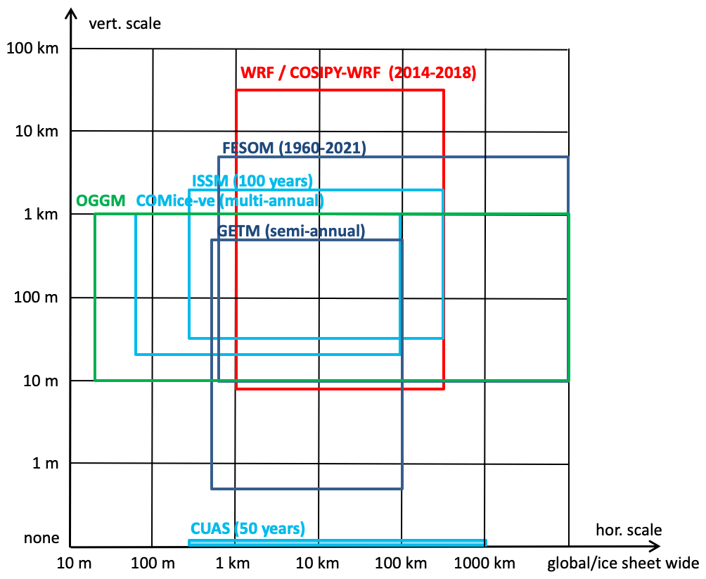
Figure 5Horizontal and vertical ranges of the ocean, glacier, ice sheet and atmospheric models used in this study. For each model (rectangles), the lower left corner denotes the horizontal and vertical resolutions (model grid size), while the upper right corner denotes the horizontal and vertical extents of the model domains.
This section presents the main results of individual GROCE studies, starting with atmospheric and ice surface processes, then moving onto glacier and solid Earth aspects and finally to ocean impacts. We will also explore individual causal relationships between these spheres. For a large part this is based on previously published results; however here we also explore the connections between them, partly based on updated datasets and newly composed figures.
4.1 Atmospheric processes and effects on the glacier surface
Using a combination of the data described in Sect. 3.1, a surface air temperature (Ta) increase of 3 °C over 1979–2017 was identified (Turton et al., 2019). This tendency agrees with yet exceeds the global trend clearly. Interestingly, significant winter temperature variability is noted with high-amplitude short-lived events (Ta>10 °C over 48 h) occurring each year between November to March over the study period. These have been linked to two mechanisms: (1) warm-air advection and (2) mixing from katabatic winds. Over 15 % of these warm-air events were found to occur in March and could result in a short period of ice melt as Ta increases along with solar radiation. On the other hand, Ta varies little within the summer season, which has been attributed to high pressure over Greenland and katabatic winds dominating the wind direction. Turton et al. (2021a) examined interannual summer temperature variations and their link to the areal extent of supraglacial lakes or surface melt ponds in the region for 2016–2019. The above-average air temperatures of 2016 and 2019, along with a number of rain events, led to extensive supraglacial lake formation up to elevations of 1600 m. Colder summers with a large accumulated snowpack, for instance in 2018, led to a limited formation of supraglacial lakes, limited to elevations of 800 m. These relationships are also evident with the new lake volume data (see Fig. 6). Furthermore, a comparison of these findings with the total area of lakes from the early 2000s (Sundal et al., 2009) points to an inland expansion and increase in area.
4.2 Atmosphere-driven changes in the climatic mass balance
By applying the high-resolution NEGIS_WRF atmospheric data to the COSIPY model (Sect. 3.1) for 2014–2018 at 1 km resolution, the simulations revealed strong interannual variability in the CMB (Blau et al., 2021). The 4-year mean specific CMB of 79NG in the defined region (here, inland to ∼ 30° W; light-blue shading in Fig. 3) amounts to a mass loss of 744 mm a−1, which is driven by runoff of meltwater produced at the surface or inside the snow layers (evaporation is negligibly small). However, as illustrated in Fig. 6, the annual CMB range showed mass losses from as much as 1049 mm (2016/17) down to 120 mm (2017/18). The strong 2016/17 mass loss was associated with strong surface melt that enhanced the ablation and runoff. The difference in surface albedo was found to be a major factor between contrasting CMB years (Blau et al., 2021); in 2018 for example, high albedo was driven by higher accumulation (snowfall) during summer (including the early ablation season) due to the lower air temperatures, which resulted in a higher snowfall fraction and reduced volumes of supraglacial lakes (Fig. 6). Hence, the combined summer air temperature and timing of precipitation are necessary to explain CMB and surface melt variability sufficiently.
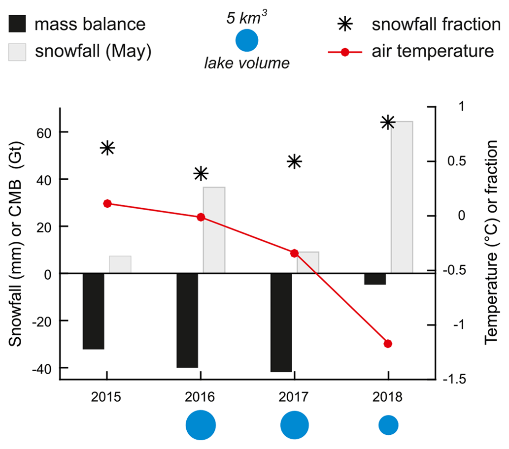
Figure 6Area-wide climatic mass balance (October of previous year to September of current year), area-averaged 2 m air temperature and snowfall fraction (June–July mean) and snowfall amount (May), and daily max lake volume (available since 2016; see Sect. 4.3) of the 79NG area for the period of 2014/15 to 2018 (when datasets overlap). Note that in the main text, CMB is given in mm a−1 rather than Gt a−1. The lake volume data have not been previously published, mass balance data are from Blau et al. (2021) and the remaining (meteorological) data are from Turton et al. (2020).
4.3 Supraglacial lake volume evolution
Supraglacial lakes are one phenomenon at the atmosphere–glacier interface, as mentioned in Sect. 4.1. Here, the combined effect of air temperature, snowpack thickness and rainfall on the development rate of supraglacial lakes is directly observed. Melt seasons with a combination of higher air temperatures, thinner snowpack or more rainfall lead to larger average lake areas and a more widespread distribution of lakes at higher altitudes. In Hochreuther et al. (2021), the total lake area upstream of the 79NG and ZI grounding lines (displayed in Fig. 3 as pink shading) is extracted and tracked over each of the investigated melt seasons. The method described in Sect. 3.3 was then applied to the lake area to derive the daily lake volume over this region over the 2016 to 2022 melt seasons (Fig. 7). The average maximum (peak) lake volume is 7.97 ± 1.96 × 10⁸ m3 (1 standard deviation) over all considered years. Most years tend to reach a fairly similar maximum daily lake volume, with the exception of 2018, which was a particularly cold and dry year. Each melt season, however, exhibits distinct lake volume accumulation and draining trends. For example, the 2020 and 2021 melt seasons have similar lake volumes of around 8.60 × 10⁸ m3 on 3 August; however, the 2020 melt season accumulates lake volume earlier and shows roughly double the meltwater volume on 25 July than that of 2021. Additionally, in most years the peak lake volume is maintained for several days only; however, in 2016 the peak of 8.76 × 10⁸ m3 is maintained for a few weeks.
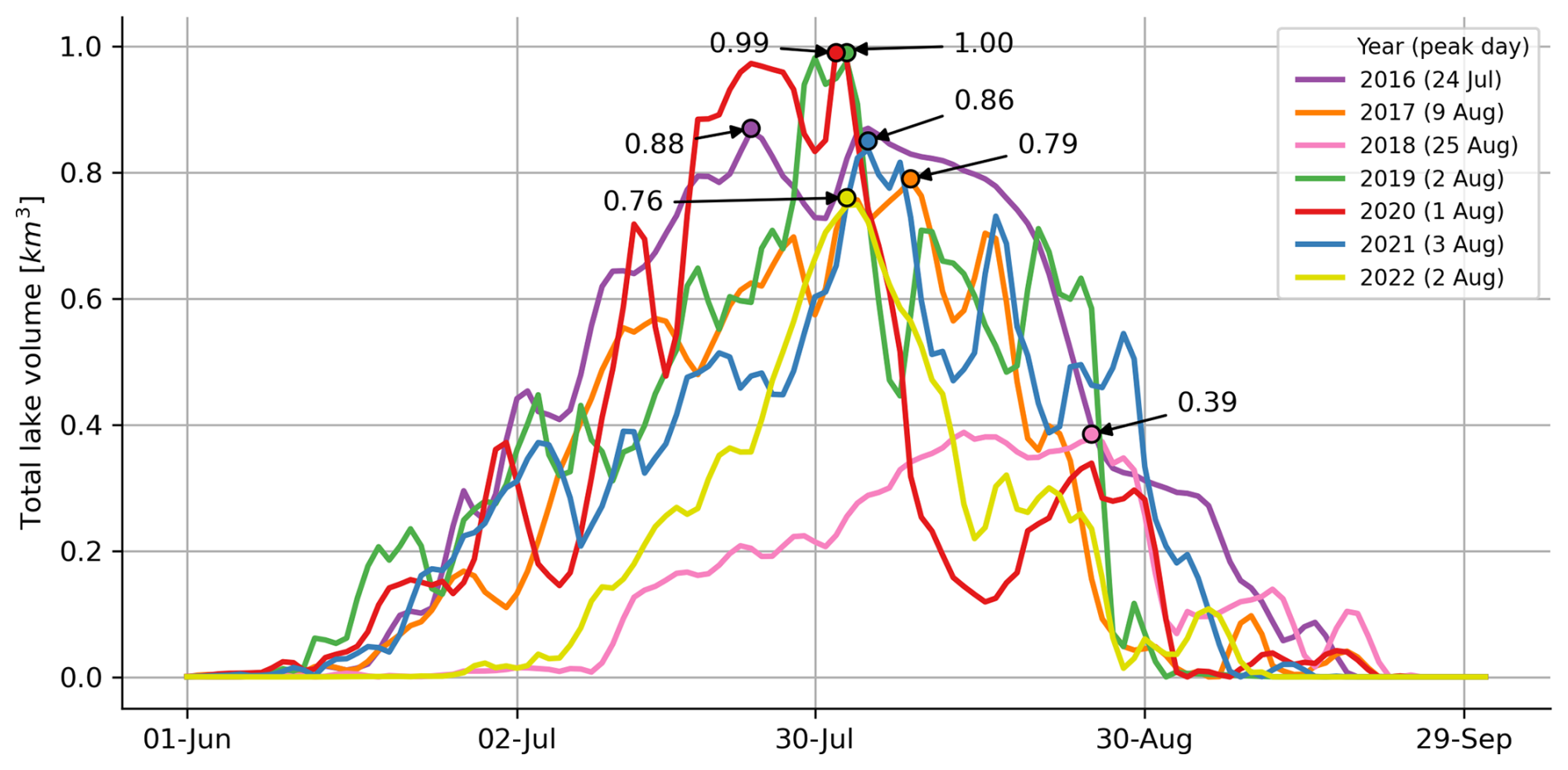
Figure 7Daily lake volumes upstream of the 79NG and Zachariæ Isstrøm grounding lines throughout the 2016 to 2022 melt seasons. The peak lake volume is marked by a dot for each year, with the corresponding date of the peak given in the legend. The dataset shown here has not been previously published.
4.4 Tidal response of 79NG
We now move from surface processes to the dynamics of 79NG. Comparing simulated and observed horizontal and vertical displacements of 79NG over a tidal cycle revealed that the representation of the ice properties by a Maxwell viscoelastic rheology is required in the model, since a purely viscous material is not sufficient to describe the response of glacier ice to tidal forcing in a realistic way (Christmann et al., 2021). In addition, tidal forcing leads to an alteration of the subglacial water pressure, which subsequently affects glacier motion due to changes in lubrication and, consequently, sliding speed. This effect is pronounced up to a distance of 10 km upstream of the grounding line, where the contribution of vertical shear to overall motion is vanishing. Both viscous and elastic deformation are largest in the vicinity of topographic changes that initiate changes in stress. The elastic contribution is persistent and makes up 6 %–30 % of the strain in our simulation experiment. Furthermore, the location of massive crevasse fields, which represent the solid nature of ice, are consistent with locations of high elastic strain.
4.5 Determination of frontal positions of 79NG and ZI
The analysis of the Landsat imagery clearly shows that the evolution of the calving-front positions of these two neighboring glaciers is completely different. The frontal position of ZI exhibits a retreat of about 7 km from March 2013 to October 2021 with a distinct seasonal signal (Fig. 8, lower right panel). In contrast to that, 79NG maintains its front more or less at the same position (Fig. 8, upper right panel). However, events of advance followed by iceberg breakups can be detected. The frontal retreat of ZI is in accordance with its significant mass-loss rate, which is about 3.5 times larger than that of 79NG (Sect. 4.7).
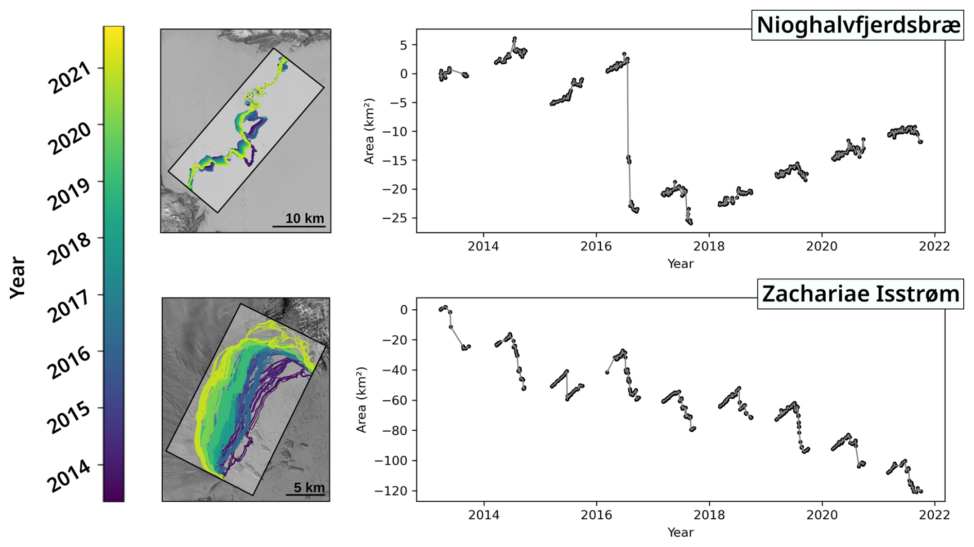
Figure 8Time series of frontal positions generated by our deep neural network for 79NG and ZI. On the left, respective sections of Landsat images for both glaciers show the calving-front trajectories color-coded for the year of observation. Note the different scales of the satellite images. The corresponding time series of the area change are plotted on the right, where the zero ordinate refers to the initial observation in March 2013. Here, calving-front positions are marked with a black dot and solid lines connect entries each year. In order to visualize the much smaller changes in the frontal position of 79NG in contrast to those of ZI, the ordinate axes of the two right-hand graphs have different scales. The figure was adapted and modified from the original version in Loebel et al. (2024).
4.6 Sensitivity of the 79NG ice discharge to the ice tongue extent
We investigated the impact of a possible disintegration of the floating tongue of 79NG on the solid-ice discharge based on a high-resolution setup of the ISSM model (Humbert et al., 2023). For 79NG Mouginot et al. (2015) provide an annual mean estimate of ice discharge across the grounding line of 12.0 ± 0.8 Gt a−1 for the period of 2010–2015 based on remote sensing data. Our ISSM-based reference simulation (init simulation shown in Fig. 9) yields an equilibrium ice discharge of 11.9 Gt a−1, which is comfortably within the error bars of the remote-sensing-based estimate.
We found that a complete loss of the floating part approximately doubles the discharge of ice across the grounding line (Fig. 9). Comparing the small change in discharge detected by Mankoff et al. (2020b) between 1986–2020 with our simulations, we conclude that, although the floating tongue of 79NG has thinned considerably (Mayer et al., 2018; Khan et al., 2022b), the buttressing still prohibits a major speedup. Only for retreats reducing the length of the ice tongue to less than 40 km does the discharge start to accelerate (experiments calv-fjord and collapse). The basal topography inland, with a steep step at a distance of about 20 km upstream of the grounding line, attenuates the effect of the loss of the floating tongue far inland.
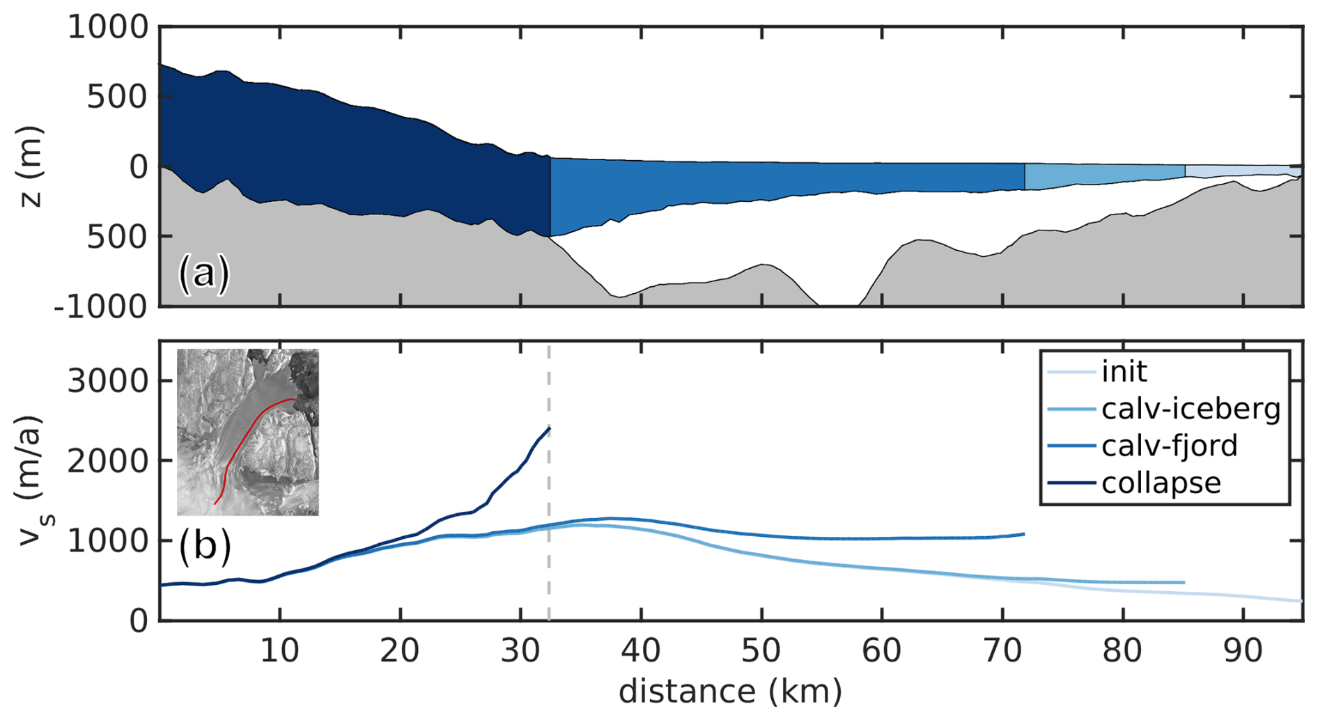
Figure 93D ice-flow simulation results along a southeastern flowline (see inset in b for the location) for the four experiments of init, calv-iceberg, calv-fjord and collapse (a full collapse of the floating tongue) (from light to dark blue, respectively). Panel (a) shows the geometry, and panel (b) shows the simulated velocities vs. The dashed gray line in (b) indicates the location of the grounding line. This figure extends the dataset published by Humbert et al. (2023).
4.7 High-resolution mass balance of the Greenland Ice Sheet
The combination of satellite gravimetry and altimetry yields a refined and improved estimate of the ice mass change at a high resolution in the working area (Fig. 10) (Kappelsberger et al., 2020, 2021). While the higher resolution is facilitated by satellite altimetry, satellite gravimetry constrains the mass balance estimate towards a physically more reliable solution, since GRACE–GRACE-FO measurements directly sense mass change. Further, the combination of the two methods maintains the spatial pattern of the altimetry input, which is a significant improvement over the gravimetry-only estimate in terms of the spatial resolution and allocation of mass changes to single glaciers (Kappelsberger et al., 2021). A major advantage of the combination method is that the contribution of the peripheral glaciers is reliably considered, which makes up more than 10 % of the entire Greenland mass balance (Sect. 4.9). This is also important for obtaining a correct mass change distribution over the different catchment areas and regions of the peripheral glaciers. The estimate from the altimetry–gravimetry combination for the time period July 2010 to June 2017 yields a mass-loss rate of −3.7 ± 1.3 and −0.9 ± 0.4 Gt a−1 for the drainage basins of ZI and 79NG, respectively. For comparison, for the same period the overall Greenland ice mass trend is −233 ± 43 Gt a−1, which is comparable to other recent estimates. Regarding the ice mass trend 87 % is contributed by the Greenland Ice Sheet and 13 % is contributed by peripheral glaciers (Kappelsberger et al., 2021).
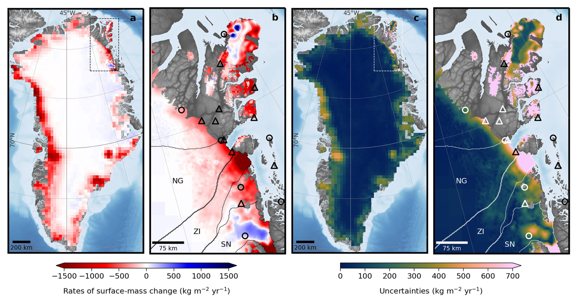
Figure 10Surface mass change rates from the combination of satellite gravimetry and satellite altimetry for (a) all of Greenland and (b) the working area in northeast Greenland, with (c, d) related uncertainties. Time period: July 2010–June 2017. NG: 79N Glacier, ZI: Zachariæ Isbræ, SN: Storstrømmen. Locations of the GNSS sites are given by triangles (TUD Dresden) and circles (GNET) (cf. Figs. 3 and 4). Figure originally published by Kappelsberger et al. (2021).
4.8 Bedrock displacement rates inferred from GNSS and the response of the solid Earth to present-day ice mass changes
From the analysis of the GNSS measurements at the individual TUD and GNET sites (Fig. 3) we inferred bedrock displacement rates (Kappelsberger et al., 2021). Here, especially the uplift rates (Fig. 11) are of great relevance, ranging between 5 mm a−1 and a maximum of almost 9 mm a−1 in west Lambert Land. The uplift rates contain both the long-term GIA effect and the elastic response due to present-day ice mass change. The GNSS site in west Lambert Land is situated close to ZI. It features the largest contemporary ice mass change in the region, which is reflected in the largest observable elastic response in NE Greenland. Therefore, a permanent GNSS site was set up at this location in July 2022 to continue the time series and resolve seasonal and interannual signal parts of the solid Earth response.
The elastic response of the solid Earth was calculated based on the refined present-day mass change estimate (Fig. 11; Kappelsberger et al., 2021). This calculation also accounts for load variations in the surrounding ocean as well as for mass redistributions on a global scale, which jointly can account for up to 10 % of the entire elastic effect (Kappelsberger et al., 2021). The largest elastic displacement rate (13.8 mm a−1) was obtained near the front of ZI (Fig. 11). The sum of the elastic displacements and those inferred from different GIA models could then be compared with the GNSS-inferred uplift rates. From that validation it turned out that the GIA models by Caron et al. (2018), Lecavalier et al. (2014) and Khan et al. (2016) are compatible with our results inferred from the combined mass change estimate and the GNSS measurements (Fig. 11). These three GIA models predict a relatively small GIA signal in NE Greenland, with rates at the GNSS sites ranging from 0.7 to 4.4 mm a−1. While for the model by Khan et al. (2016), a good agreement was expected since it is based on the GNET data, for the other two models the agreement is remarkable. Lecavalier et al. (2014) presented a regional model based on comprehensive records of past ice extent and relative sea-level (RSL) data. Caron et al. (2018) included only a few RSL data points and no GNSS-inferred rates in Greenland at all (Kappelsberger et al., 2021). However, since the determination of GIA represents a highly non-unique problem, research into better constraining both the ice-load history and the rheology of Earth will remain a challenge, forming the two primary quantities for GIA forward modeling.
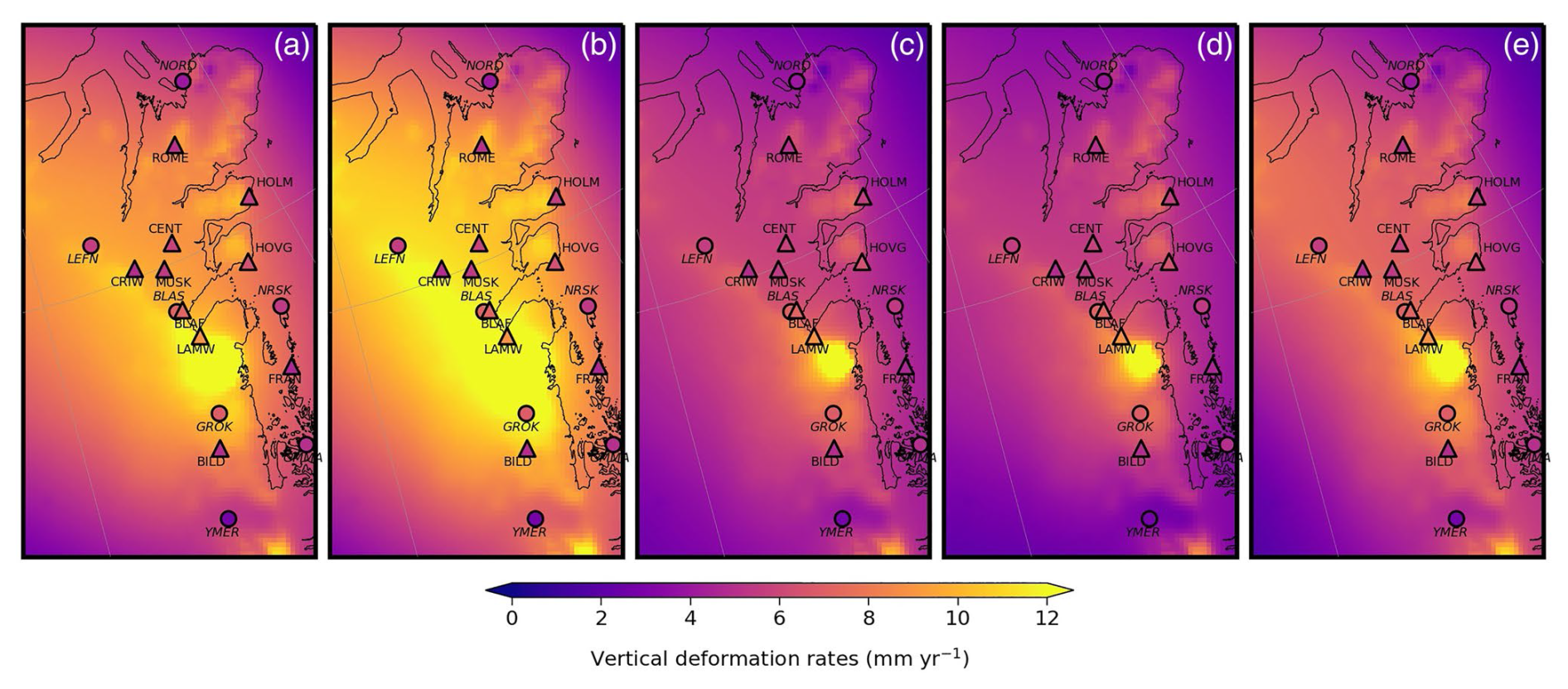
Figure 11Total vertical displacement rates inferred from the sum of the elastic (instantaneous) response (calculated based on the mass change rate from altimetry–gravimetry combination) and the viscoelastic (long-term) response predicted by different GIA models: (a) A et al. (2012), (b) Peltier et al. (2015), (c) Caron et al. (2018), (d) Lecavalier et al. (2014) and (e) Khan et al. (2016) (GNET). GNSS-inferred vertical displacement rates, inferred for the time period of June 2008 to July 2017, are shown in the same color scale, for TUD Dresden sites (triangles) and GNET sites (circles). Figure originally published by Kappelsberger et al. (2021).
4.9 Mass balance of peripheral glaciers in northeast Greenland
The differences in the spatial resolution of the climate drivers (input data) play a major role in the simulated glacier and hydrologic outputs from OGGM (Sect. 3.9). The freshwater runoff contributions from FIIC were 11.40, 9.57 and 9.93 Gt a−1 when simulated using the CRU, ERA5 and NEGIS_WRF datasets as atmospheric boundary conditions, respectively, during 2014–2017 (Fig. 12d–f). Despite their different spatial resolutions, there were no significant statistical differences in freshwater runoff contributions across datasets. However, during the mass balance calibration process within OGGM, the coarse-resolution datasets (CRU and ERA5) were corrected using precipitation scaling factors (2.5 and 1.6, respectively). High-resolution precipitation based on NEGIS_WRF, by contrast, was sufficient to calibrate the mass balance without applying corrections, increasing confidence in these results.
The grounding lines of the ice shelf in the two basins of FIIC showed a slight advance during the 1996–2001 surge activity (Svalbard type). Since 2001 the grounding lines of basins 2 and 3 have retreated by 2.2 ± 1.3 and 2.7 ± 0.9 km (Möller et al., 2022), suggesting an ongoing mass loss in the area. This finding is consistent with the observations of Kappelsberger et al. (2021) (Fig. 12c). During the surges, ice discharge from basins 2 and 3 reached amounts of 0.145 and 0.119 Gt a−1. Afterward, the discharged ice masses rapidly decreased to a distinctly lower level of just 10 % (basin 2) and 4 % (basin 3) of their maximum values. OGGM simulations revealed a total mass loss from FIIC of 2.8 ± 0.7 Gt a−1 from 2010 to 2019.
The peripheral glaciers in NE Greenland underwent a significant mass change, with a calculated mass loss of 8.1 ± 4.3 Gt a−1 between 2010 and 2019. These simulated mass changes agree with the estimates of Khan et al. (2022b). The peripheral glaciers in NE Greenland will lose significant volume in the future. The remaining volume is predicted to be 78 ± 4 % for SSP126 (low-emission Shared Socioeconomic Pathway scenario) and 61 ± 9 % for SSP585 (high-emission scenario) by 2100 compared to 2019 (Fig. 12g). Based on the future projections, the total mass loss from the peripheral glaciers of NE Greenland is 5.15 ± 0.88, 6.44 ± 1.19, 7.94 ± 1.73 and 9.04 ± 2.16 mm sea-level equivalent (SLE) under SSP126, SSP245, SSP370 and SSP585, respectively, by 2100 compared to the mass in 2019 (Fig. 12h). The values in parentheses represent the actual sea-level rise (dotted lines in Fig. 12h) after excluding the mass loss below the water level. The uncertainty in the projections was higher for high-emission scenarios.
Projections of freshwater contributions from peripheral glaciers into the ocean are essential for understanding how the interactions between glaciers and the ocean will evolve in a warming climate. Increased meltwater will eventually end up in the ocean, altering the density distribution within the fjords and, thereby, fjord circulations and submarine melt rates (Hopwood et al., 2020; Henson et al., 2022). Total liquid freshwater contributions from NE Greenland (excluding submarine melt and calving fluxes) to the ocean are projected to be 3922 ± 315 Gt (SSP126) and 5576 ± 826 Gt (SSP585) during 2020–2100. Of specific interest is the year of peak water, which is the point in time when total annual runoff from a glacier reaches its temporal maximum under a given climate scenario. In high-emission scenarios, this point in time is usually reached later than in low-emission scenarios, since the excess melt can continue to an increase over the rest of the 21st century. For the lower-emission scenarios, the glacier would start to approach a new equilibrium within the 21st century, which reduces the runoff. The peak waters are projected to occur in the years 2053 ± 22 (51.8 ± 16.6 Gt a−1), 2070 ± 19 (54.5 ± 12.9 Gt a−1), 2082 ± 17 (80.4 ± 17.9 Gt a−1) and 2080 ± 19 (79.2 ± 19.3 Gt a−1) under SSP126, SSP245, SSP370 and SSP585, respectively (Fig. 12i).
According to Bamber et al. (2018) the bulk (solid and liquid) freshwater flux from Greenland into the ocean has increased from the 1980s to the late 2010s by 400 Gt a−1 (corresponding roughly to 40 %). Given that the rate in the late 2010s is still just 20 % of the ocean freshwater flux from the Arctic Ocean into the North Atlantic, the impact of the Greenland freshwater flux on the Atlantic thermohaline circulation has likely not yet been significant (Böning et al., 2016). At the same time freshening of the surface waters by Greenland freshwater has already been shown to episodically counteract the effect of wintertime cooling in terms of deepwater formation in the North Atlantic (Lozier, 2023) such that the Greenland impact might be emerging (Böning et al., 2016; Lozier, 2023). Martin et al. (2022) suggest that an increase in Greenland freshwater fluxes by roughly 1600 Gt a−1 might reduce Atlantic thermohaline circulation by not more than 15 %. Projected peak freshwater fluxes of northeast Greenland peripheral glaciers of 50–80 Gt a−1 occurring in the second half of this century may contribute to such a Greenland-wide impact but are unlikely to be of leading importance.
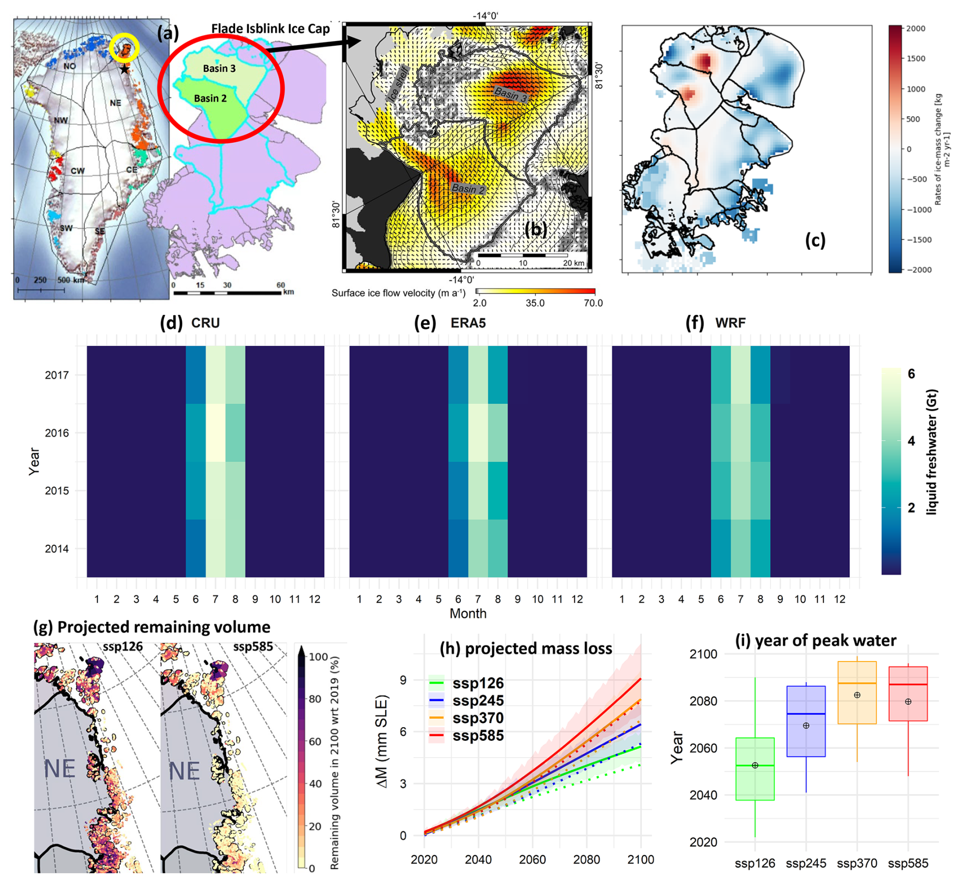
Figure 12(a) Greenland peripheral glaciers and new outlines of the Flade Isblink Ice Cap (FIIC). Glaciers are highlighted in different colors for different subregions. New FIIC outlines highlighted in cyan are active marine-terminating glaciers. (b) Thick black-and-white outline represents the delineation of basins 2 and 3 that was drawn based on 2019 Sentinel-1 surface ice-flow velocities (color grid) and directions (arrows) (Möller et al., 2022). (c) Mass balance based on altimetry and gravimetry obtained from Kappelsberger et al. (2021). (d–f) Freshwater runoff, simulated using different spatial resolution forcing datasets. (g) Projected remaining volume of peripheral glaciers in NE Greenland by 2100 (for low- and high-emission scenarios) compared to the volume in 2019. (h) Projected total glacier mass loss up to 2100 (10 GCMs: mean ± 1 SD) from NE Greenland peripheral glaciers compared to 2019. The dotted lines represent the mean sea-level rise after subtracting the mass loss below water level under SSPs. (i) Projected years of peak water (mean ± 1 SD) for the freshwater runoff contributions from peripheral glaciers of NE Greenland under SSP126, SSP245, SSP370 and SSP585 (10 GCMs: mean ± 1 SD). The analyses displayed in panels (d) to (i) are part of Shafeeque et al. (2024).
4.10 Insights of ocean circulation into the cavity by observations and models
After having discussed ice sheet and glacier processes relevant to the mass balance of the 79NG system and adjacent peripheral glaciers, we move on to ocean impacts (i.e., the ocean-driven melt in Sect. 4.10 to 4.12 and impacts of the meltwater on the ocean in Sect. 4.13). A mooring-based time series of ocean velocity, temperature and salinity near the calving front of 79NG from 2016 to 2017 (location given as green dots in Figs. 3 and 4) indicates the existence of a year-round bottom-intensified inflow of warm AIW into the cavity through a narrow channel across a chain of small islands to the calving front, suggesting a year-round ocean-driven basal melt takes place (Schaffer et al., 2020). This consistent AIW inflow entering the cavity as a bottom-intensified dense water plume is confirmed by continued hydrographic observations at the calving front until 2022 (see velocity and temperature observations downstream of the sill at the calving front in Fig. 13a). The combination of the observations with a bathymetric survey reveals that this inflow is constrained via hydraulic control by a topographic sill located several kilometers upstream of the calving front (for the process, see Fig. 2), meaning that the height of the warm and saline AIW layer above the submarine sill controls the magnitude of AIW volume (and heat) transport into the cavity of 79NG (McPherson et al., 2024). Temperature profiles at the neighboring ZI suggest that ocean heat transport here is similarly controlled by a near-glacier sill (Schaffer et al., 2020). Near-glacier sill-controlled ocean heat transport thus plays a crucial role in glacier stability. Based on the same mooring data, von Albedyll et al. (2021) found that the deep AIW inflow is connected to a shallow outflow of modified (cooled and freshened) AIW on timescales exceeding 1 month, with exchange flow variability being intensified in wintertime. The extent to which the intraseasonal variability is relevant to modulating melt rates is unclear, as the residence time of seawater in the cavity exceeds 6 months.
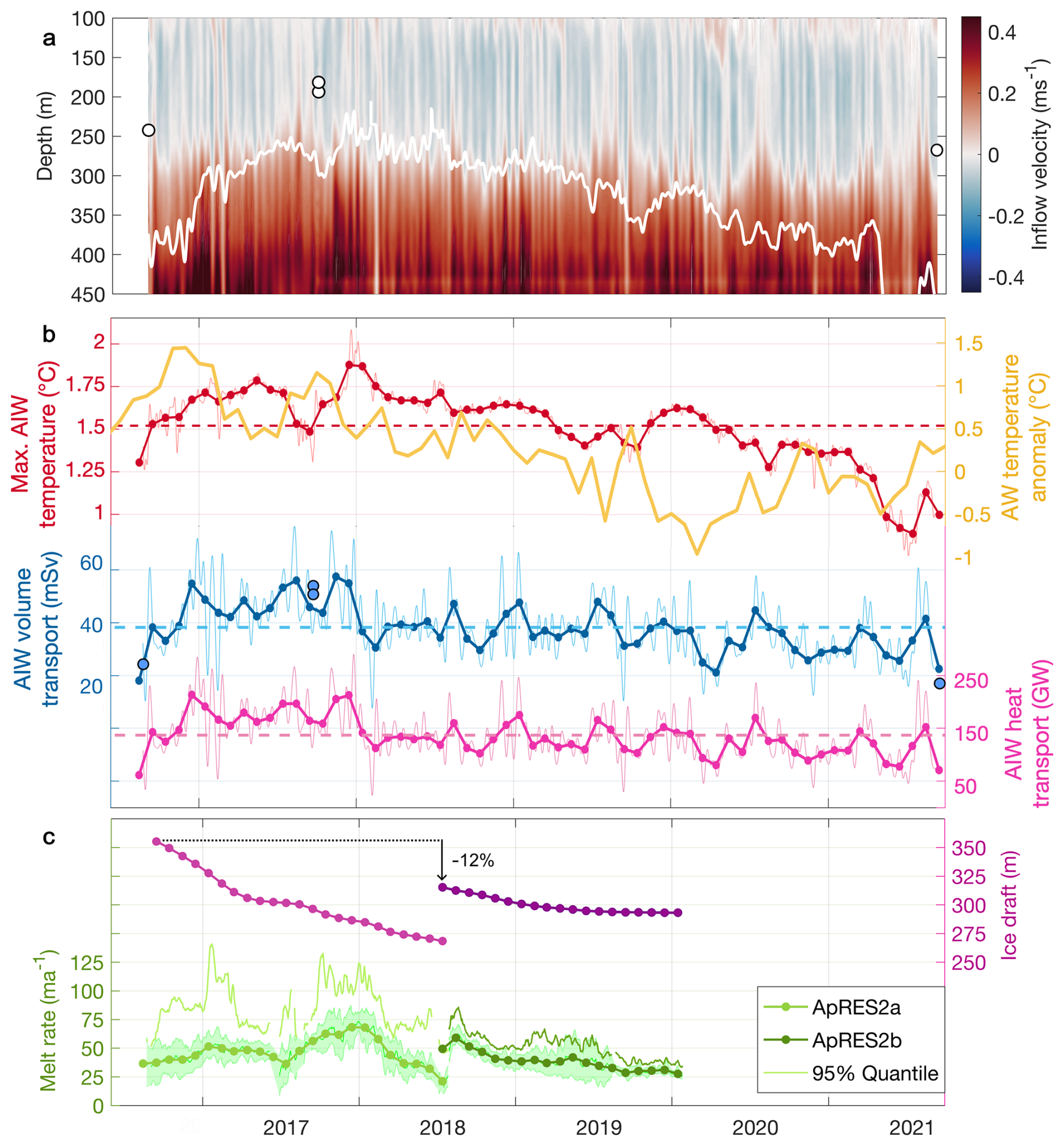
Figure 13Evolution of the AIW inflow to the cavity below 79NG. (a) Inflow (red) and outflow (blue) velocities recorded by a mooring deployed at the 79NG calving front (Fig. 4). The white line is the depth of the 1 °C isotherm. (b) Time series of weekly and monthly maximum AIW temperature (red), the near-surface mean AW temperature anomaly in the WSC (east Fram Strait) from mooring observations (yellow), and AIW volume (blue) and heat (pink) transport into the cavity. Dashed horizontal lines are the respective mean values. (c) Local ice draft (purple) and basal melt rate (green) time series of the ApRES measurements (monthly means). The two deployments were between 2016–2018 (lighter colors) and 2018–2020 (darker colors). The shaded area around the melt rates marks the range between the 25 % and 75 % quantile, and the thin line marks the 95 % quantile. Note that the maximum grounding depth of 79NG slightly exceeds 600 m (Zeising et al., 2024a), while the ice draft shown here corresponds to the local ice draft at the position of the instrument. Circle markers in (a) denote the bifurcation depths from the cross-sill CTD (conductivity–temperature–depth) profiles and in (b) denote the volume transport estimates derived from these CTD profiles by applying hydraulic control theory. Figure adapted from McPherson et al. (2024) published under the AAAS license (no. 5950111248607).
As oceanographic observations are mostly constrained to the calving front and open ocean, we make use of ocean models to study the ocean circulation inside the glacier cavity. The 2D fjord model (2D in the x–z plane) features both an along-fjord bathymetry and an ice tongue geometry similar to that of 79NG (Reinert et al., 2023). The 2D fjord model reveals a meltwater plume that forms on the underside of the floating ice tongue, initiated by subglacial runoff discharged at the grounding line. It rises along the ice tongue, since it is fresher and thus lighter than the surrounding AIW in the cavity (see schematic in Fig. 2). Being equipped with adaptive vertical coordinates (Sect. 3.13) and featuring 100 vertical layers, the model is ideally suited to simulate the small-scale turbulent exchange processes between the meltwater plume, the ice base above and the AIW layer below. The 3–5 m thick plume causes basal melt of the ice tongue due to friction-imposed ocean heat flux at the ice–ocean interface. The meltwater is absorbed by the plume and increases its buoyancy. On the other hand, the plume becomes less buoyant due to the entrainment of AIW from below (Burchard et al., 2022). Eventually, the plume water reaches the same density as the surrounding AIW.
It detaches from the ice tongue around 42 km downstream of the grounding line, where the ice draft is 95 m (exceeding the ice draft at the calving front by just 20 m); propagates horizontally away from the ice (Reinert et al., 2023); and transports glacially modified (i.e., cooled and freshened) water out of the fjord (Fig. 2) at mid-depths (95 to roughly 250 m). The depth range of exported waters from the cavity is supported by our observations of the subsurface distribution of helium and neon near the calving front (Fig. 16c; Sect. 4.13).
Our 3D ocean–sea ice model, featuring a horizontal mesh resolution of 700 m in the cavity and its surrounding, reveals that the warm and salty AIW enters the cavity through its deepest channel as a bottom-intensified gravity current (Wekerle et al., 2024), in agreement with Schaffer et al. (2020). The warm AIW then circulates cyclonically around the cavity. The year-round inflow of AIW results in ocean temperatures above the freshwater freezing point in the cavity, leading to basal melt (as in the 2D fjord model). Both basal meltwater and subglacial discharge which enters the cavity in the summer months across the grounding line sustain a meltwater plume which entrains ambient water as it rises. Driven by buoyancy and deflected by the Coriolis force, the plume accelerates along the southern flank of the cavity, detached from the ice base. As a consequence, the plume features a width of just 3 km residing between 100 and 280 m depth. The plume significantly widens horizontally near the calving front and transports the meltwater out of the cavity. The ocean circulation inside the cavity is thus clearly affected by the Coriolis force, deviating strongly from a 2D estuarine circulation. The basal melt rates computed by our model simulations are discussed in Sect. 4.11 below.
4.11 Basal melt of the floating tongue of 79NG
The heat transport associated with the flow of AIW into the cavity leads to year-round melt at the base of the floating glacier tongue (Schaffer et al., 2020). It is the major contribution to the observed thinning of the ice tongue of 79NG (Wilson et al., 2017; Mayer et al., 2018). The warming of the AIW and lifting of the 1°C isotherm, defining the interface between the AIW and outflow, by 200 m from August 2016 to December 2017, led to a more than doubling of the AIW volume transport into the cavity from 19 to 55 mSv (millisverdrup, 1 Sv = 1×10⁶ m3 s−1; Fig. 13a, b). The variability in the heat transport into the cavity is dominated by fluctuations in the strength of the inflow (featuring a time mean value of 36 ± 10 mSv from 2016–2021), leading to a corresponding increase in heat transport from 65 to 214 GW (McPherson et al., 2024). Subsequently, AIW temperatures strongly reduced by 0.65 °C and the AIW layer thinned by 190 m (Fig. 13a, b). Correspondingly, the heat transport also decreased at a rate of 40 GW a−1; this abrupt cooling of AIW was attributed to blocking-related cold-air anomalies that enhanced the ocean heat loss of AW upstream in Fram Strait and further south in the Norwegian Sea and slowed down the circulation, intensifying the AW cooling (McPherson et al., 2024).
Time series measurements of basal melt in close vicinity of the grounding line were carried out using ApRES devices (Zeising et al., 2024a; see also Fig. 4). The authors found that the bottom side of 79NG’s floating tongue has a relatively rough surface so that the ApRES measurements of basal melt record not only nadir reflections but also side reflections, affecting the ability to constrain the melt rates. Figure 13c presents a time series of basal melt rates inferred from the ApRES measurements and reveals strong temporal variability, with no clear seasonal cycle. The difference between the median and 95 % quantile also reflects the spatial variability as a large difference indicates the presence of low and high melt rates near the measurement site at the same time due to changes in basal topography. The median melt rates increased from 37 m a−1 in October 2016 to 73 m a−1 at the end of 2017, though maximum values exceeded 120 m a−1 (95 % quantile) recorded 7.5 km downstream of the grounding line. From early 2018 onward melt rates then steadily decreased to January 2020, reducing by over 50 % from the 2017 peak, with reduced spatial variability. The reduction coincided with the observed decline in the AIW temperature near the calving front, manifesting itself in the deepening of the 1 °C isotherm (Fig. 13a, b). McPherson et al. (2024) found that changes in the temperature of the inflowing AIW at the calving front are expected to drive changes in the melt rate at the grounding line a few months later (see also Sect. 4.12).
As the melt rates derived from ApRES measurements are restricted to single locations close to the grounding line, we now analyze maps of basal melt rates derived from different models and from remote sensing data (Fig. 14). A common feature is the increased melt rate close to the grounding line and its concentration in the southern part. Based on satellite imagery collected between 2011 and 2015, Wilson et al. (2017) estimated an area-averaged melt rate of 7.4 m a−1 (assuming an ice shelf area of 1600 km2), with highest values of 50–60 m a−1 close to the grounding line (Fig. 14d). In the 3D fjord model (Fig. 14b), we obtain area-averaged melt rates of 10.1 m a−1, close to the value of 10.4 ± 3.1 m a−1 derived from mooring-based observations at the calving front for the period of summer 2016 to summer 2017 (Schaffer et al., 2020). The 2D fjord model (Fig. 14a) produces an area-averaged melt rate of 12.3 m a−1. The global 3D ocean–sea ice model (Fig. 14c) simulates a mean melt rate of 10.3 m a−1. The satellite-derived melt rates by Wilson et al. (2017) (Fig. 14d) thus yield a lower mean melt rate than our estimates based on numerical models or observed hydrography. The satellite retrievals assume a hydrostatic equilibrium over the entire floating ice tongue, which may not be well justified close to the grounding line, where the highest melt rates occur. However, it has to be noted that the basal melt rates obtained by the ocean models are also subject to uncertainties. The simulated basal melt rates were computed based on the three-equation system. An important parameter in this formulation is the basal drag coefficient, which is not well constrained by observations and sometimes used to tune the models. Indeed, sensitivity experiments showed that the magnitude of the simulated basal melt rates of 79NG strongly depends on the choice of the basal drag coefficient (Wekerle et al., 2024). Basal melt rates of 8.6 ± 1.4 m a−1, i.e., lower than our other estimates but still higher than the numbers suggested by Wilson et al. (2017), were obtained by Huhn et al. (2021a) based on measurements of helium and neon on the NE Greenland shelf and close to 79NG in summer 2016. The above melt rates in units of meters per annum (m a−1) can be converted to gigatonnes per annum (Gt a−1) and a meltwater flux in millisverdrups (mSv) by multiplication of 1.7 and 0.053, respectively. Schaffer et al. (2020) estimate the subglacial discharge of freshwater into the cavity amounts to 11 % of the basal meltwater flux, which is in rough agreement with corresponding estimates based on the 3D fjord and ocean–sea ice models. To put the above numbers of basal melt into perspective of ice discharge across the grounding line, the Mouginot et al. (2015) estimate of 12.0 ± 0.8 Gt a−1 for 79NG can be translated into a “vertical growth rate” of the ice tongue of 7 m a−1 (obtained by division by 1.7; see above). This is clearly less than any of the melt rate estimates above, confirming the observed, decadal thinning of the floating ice tongue (see also Wilson et al., 2017).
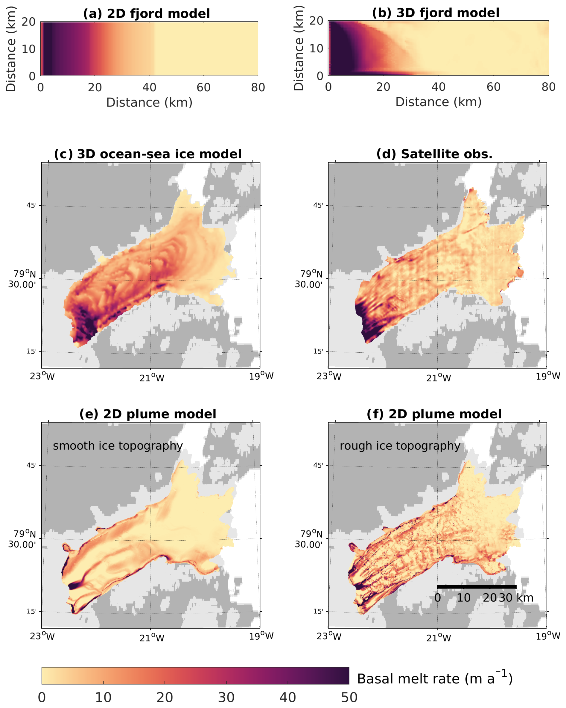
Figure 14Basal melt rate (m a−1) of the 79NG ice tongue from (a) the 2D fjord model (Reinert et al., 2023), (b) the 3D fjord model (not previously published), (c) the 3D ocean–sea ice model (FESOM2.1; Wekerle et al., 2024), (d) satellite observations (Wilson et al., 2017), and (e–f) the 2D plume model (dataset not previously published) using (e) a smooth ice base topography and (f) a rough ice base topography. The gray and light-gray backgrounds in (c)–(f) show bare land and grounded ice, respectively.
The sensitivity of basal melt rates to ocean temperature and subglacial discharge was tested with both the 2D fjord model and the 3D ocean–sea ice model (Table 1). Increasing the water temperature by 0.5 and 1.0 °C – representing realistic ranges of interannual to decadal changes (e.g., Schaffer et al., 2020, and Fig. 13) – leads to an increase in basal melt by 26 % and 52 %, respectively, in the 2D fjord model. A doubling of subglacial discharge – corresponding to the difference between a year with average and one with high discharge (see Fig. 15 for a discharge time series) – increases the basal melt by 16 %. From an ensemble of seven sensitivity experiments, Reinert et al. (2023) concluded that the basal melt rate can be best described by a function that depends on the square root of subglacial discharge and is around 7 m a−1 in the absence of discharge. These findings are consistent with results obtained from the global 3D ocean–sea ice model. Sensitivity experiments with reduced and enhanced subglacial discharge confirm the square-root relationship with basal melt (Wekerle et al., 2024). Regarding ocean temperatures, we find that mean basal melt rates follow a quadratic function of AIW inflow temperature in the 3D ocean–sea ice model. Other studies of ice shelf basal melt came to similar conclusions regarding the relationship between basal melt and thermal forcing/subglacial discharge. An above-linear dependency of basal melt on thermal forcing and a square-root dependency on subglacial discharge has been revealed for the Ryder and Petermann glaciers (Wiskandt et al., 2023; Cai et al., 2017) and for the Amundsen Sea ice shelves (Jenkins et al., 2018). For tidewater glaciers however, where the subglacial discharge can be much larger than the submarine ice melt, a cubic relationship with subglacial discharge (Slater et al., 2016) has been revealed. Moreover, the sensitivity of basal melt to the roughness of the ice base has been explored with the 2D plume model. An experiment featuring a smooth ice base geometry revealed a somewhat lower area-averaged melt rate of 4.3 m a−1 compared to that resulting from the rough geometry (8.3 m a−1; compare Fig. 14e, f). The latter features a clear imprint of the locations of the subglacial channels on the distribution of melt rates across the ice tongue (Fig. 14f).
(Wilson et al., 2017)Table 1Synthesis table containing the GROCE estimates concerning the mass balance of the NEGIS–79NG–ocean system. Numbers in the first row refer to the entries in Fig. 18.
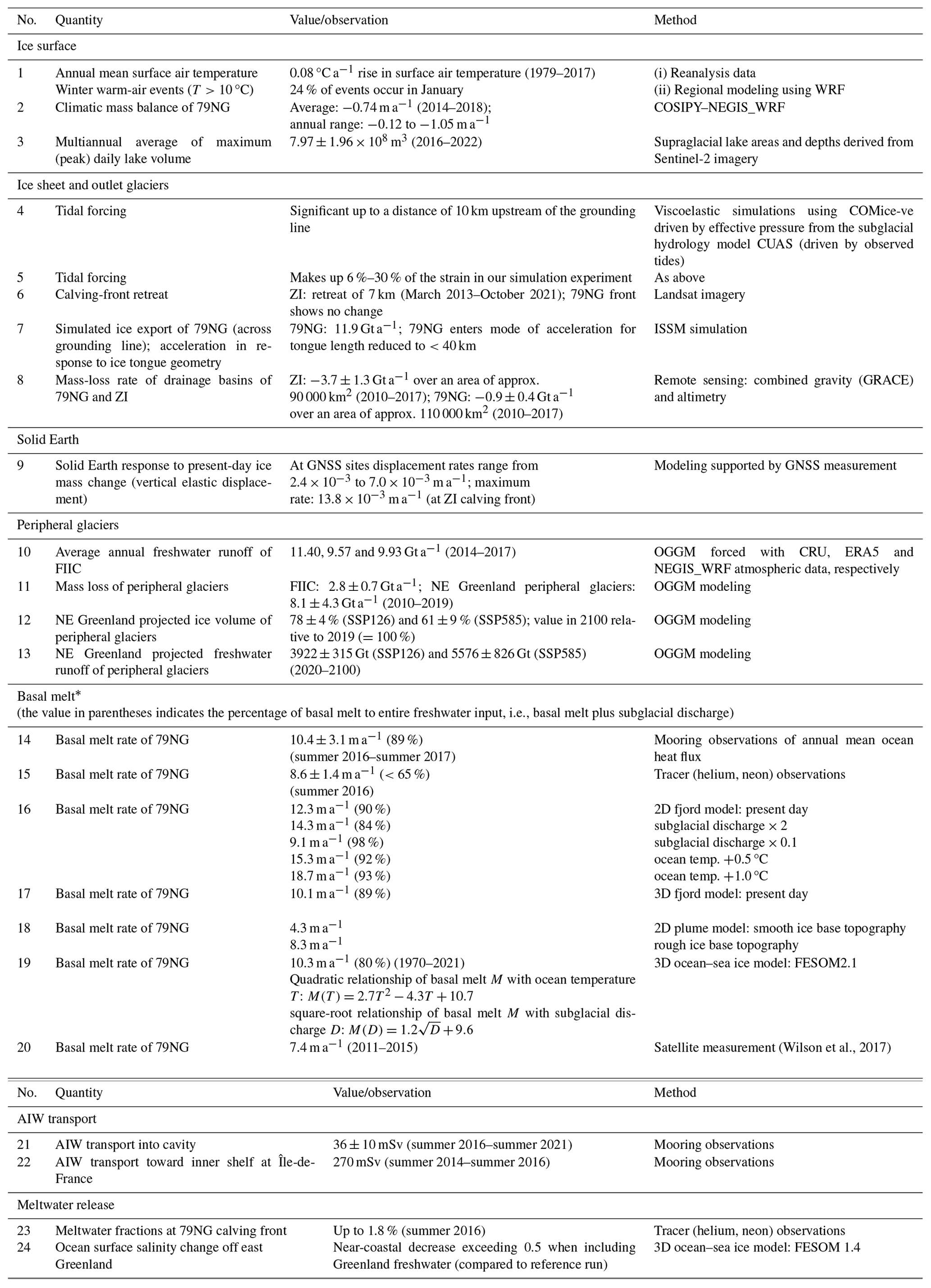
* Using the 79NG tongue base area of 1700 km2, the basal melt rates (m a−1) in lines 14–20 can be converted into meltwater volume or mass fluxes.
4.12 Origin and pathways of Atlantic Intermediate Water on the shelf of NE Greenland
Based on historical hydrographic data, Schaffer et al. (2017) demonstrated that the AIW present near 79NG was transported by an anticyclonic circulation on the NE Greenland shelf, with Norske Trough (Fig. 3) representing the inflow pathway. From the 2014–2016 mooring time series of temperature and velocity in central Norske Trough, Münchow et al. (2020) were able to identify a subsurface boundary current transporting about 0.27 Sv of AIW from Fram Strait towards the inner shelf. The intraseasonal variability in the subsurface AIW transport can be explained by topographic Rossby waves, generated by wind stress curl forcing on the Greenland shelf break; von Albedyll et al. (2021) showed the observed AIW transport in Norske Trough to co-vary with the AIW inflow into the cavity of 79NG, however, with no significant lag, suggesting fast, wave-like propagation of these fluctuations. Finally, Lindeman et al. (2020) observed that temperature anomalies obtained from the same (2016–2017) mooring at the calving front were rapidly transported into the cavity. In addition to a high degree of connectivity of AIW transports toward 79NG on intraseasonal timescales, based on the 3D ocean–sea ice model covering the time period of 1970–2021, McPherson et al. (2023b) found that the interannual variability in the AIW on the continental shelf of NE Greenland was driven primarily by the westward advection of AW from the WSC across Fram Strait. The authors show that both temperature anomalies in the WSC and wind-driven anomalies of the ocean circulation in Fram Strait contribute significantly to the AIW temperature variability on the shelf. The 3D ocean simulation also shows that not only the AIW temperature on the NE Greenland shelf but also the basal melt rates of 79NG are strongly connected to the upstream ocean conditions (Fig. 15; Wekerle et al., 2024). Simulated annual mean basal melt rates are significantly correlated with the inflow temperature at the calving front (r=0.85), whereas the correlation with the subglacial discharge across the grounding line is not significant (r=0.22).
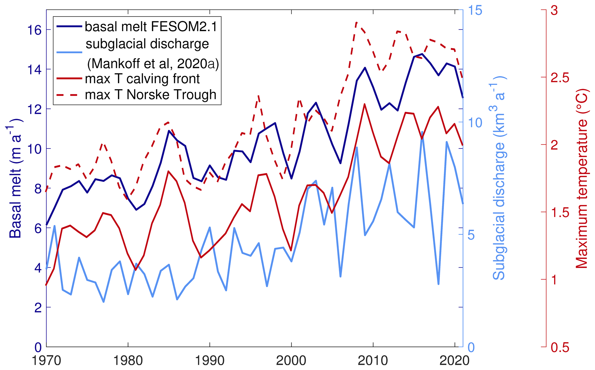
Figure 15Simulated annual mean basal melt rate (dark-blue line) and maximum AIW temperature at the calving front (red line) and in the central Norske Trough (dashed red line) from the sea ice–ocean model FESOM2.1 and subglacial discharge from Mankoff et al. (2020a) (light blue). Figure adapted from Wekerle et al. (2024).
Hydrographic data collected since the 1980s in the inflow pathway of the AIW roughly 100 km upstream of the sill at the 79NG calving front suggest that the thickness of the AIW layer on the continental shelf of NE Greenland has significantly increased over the past 2 decades (McPherson et al., 2023b). Given that the AIW inflow into the cavity is hydraulically controlled, this implies an increase in the basal melt rate of 79NG (Schaffer et al., 2020). In agreement with the observations, the 3D ocean–sea ice simulation revealed an increase in the AIW temperature at the calving front of 79NG with a trend of 0.19 °C per decade during the time period of 1970–2021 (Fig. 15). The increasing AIW temperatures are strongly reflected in simulated basal melt rates (Fig. 15), which increase by 1.38 m a−1 per decade. Wekerle et al. (2024) conclude that the temporal evolution of Atlantic Water in Fram Strait is the main driver of changes in basal melt rates of 79NG over the past 50 years. This result may predominantly hold for northeast and south Greenland outlet glaciers, while for the northwest Greenland ones, the increase in subglacial discharge may have been the dominant factor for the increased submarine melt rates at the calving fronts (Slater and Straneo, 2022).
4.13 Spreading of meltwater around Greenland
Based on a year-long record of moorings, von Albedyll et al. (2021) found that around half of the outflow of glacially modified AIW from 79NG was exported through Dijmphna Sund, with the other half going through three exchange gateways along the main calving front. By measuring noble gases, the basal meltwater contained in the modified AIW can be traced on the NE Greenland shelf (Huhn et al., 2021a; Fig. 16b, c). There it is present at the highest concentrations of basal meltwater between roughly 100 and 200 m, confirming the subsurface, density-equilibrated outflow of glacially modified waters from the cavity simulated by the 2D fjord model (and the 3D ocean–sea ice model). The basal meltwater fraction dilutes from concentrations of 1.8 % at the calving front of 79NG to non-detectable values (<0.1 %) near the shelf break. This suggests that a sizable meltwater impact on the ocean circulation should be restricted to the inner shelf. It also suggests that the basal meltwater signal observed more than 2000 km downstream in the East Greenland Current close to Cape Farewell (Kap Farvel) (Rhein et al., 2018) at the southern tip of Greenland (Fig. 1) does not originate from 79NG but rather from fjords further south.
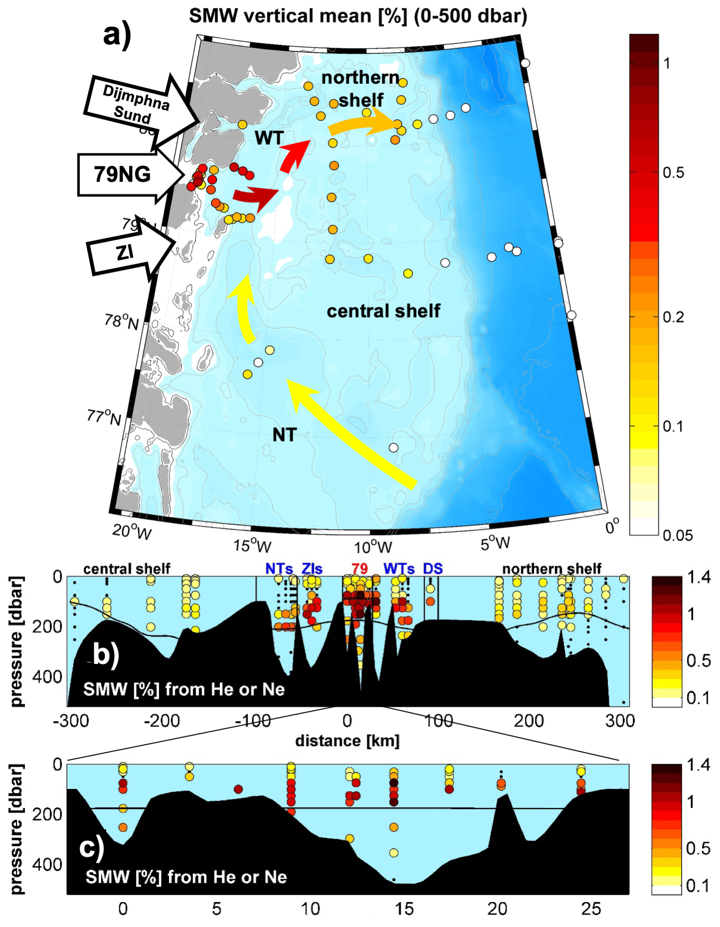
Figure 16(a) Map of the NE Greenland continental shelf with noble-gas-based vertically averaged basal meltwater fractions from the uppermost 500 dbar (data from PS100, 2016). (b) Section with noble-gas-based basal meltwater fractions, following a line from Fram Strait across the slope onto the central shelf (∼ 79° N) towards Norske Trough (NT); along the 79NG calving front, Westwind Trough (WT) and northern shelf (80° N); and ending in Fram Strait. (c) Zoomed-in representation of the same section along the 79NG calving front. Figure adapted from Huhn et al. (2021a). SMW: submarine meltwater, DS: Dijmphna Sund.
Simulations using the second setup of the 3D ocean–sea ice model (FESOM1.4; Sect. 3.13) allowed us to study the spreading of glacial meltwater on a larger scale (Stolzenberger et al., 2022), focusing not only on 79NG as a meltwater source but rather on the entire Greenland Ice Sheet. The meltwater runoff has a clearly detectable impact on the salinity and temperature distributions in the ocean surrounding Greenland. On the eastern coast of Greenland, we find a near-coastal band featuring a pronounced drop in sea surface salinity exceeding 0.5 when considering a realistic rate of Greenland freshwater runoff compared to the reference run without runoff (Fig. 17). This suggests that any anomalous circulation response to the freshening (via geostrophy) is limited to the coastal current system and does not extend to the East Greenland Current branches at the mid-shelf and shelf break. On the western coast of Greenland, the negative anomaly in salinity is present throughout Baffin Bay (not shown). Moreover, a warm anomaly of up to 0.5 °C occurs along the western coast. As we only modified the meltwater runoff between the two simulations, temperature variations are entirely due to the dynamic response of freshwater input.
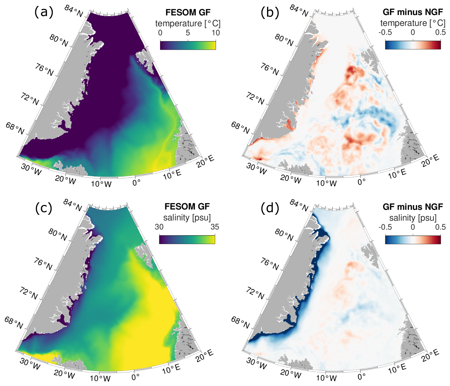
Figure 17(a, b) Surface temperature and (c, d) surface salinity in the Greenland freshwater experiment (GF; a, c) and the difference between the GF experiment and an experiment without Greenland freshwater (NGF; b, d). Blue shading represents cooling (for temperature) and freshening (for salinity) effects due to GF. The time period is 1993–2016. Figure based on model output and analysis in Stolzenberger et al. (2022).
Here we summarize our main findings with the goal of piecing together the most important estimates relevant to the mass balance of the 79NG ice–ocean system made in the framework of the GROCE project. Figure 18 and Table 1 contain this information in a condensed form. Atmospheric data reveal that the NEGIS area has experienced a multidecadal surface air temperature increase of 0.8 °C per decade (1979–2017). Accordingly, our 2014–2018 results show that 79NG clearly was in a mass-loss mode with a mean specific CMB (nearly the surface mass balance) of −744 mm a−1; year-to-year variations, however, are strong and can only be understood from the combination of summer air temperature and precipitation during the previous winter, in particular, the solid precipitation fraction, which affects the albedo. Our time series of supraglacial lake volumes for 2016–2022 shows that the annual mean CMB and annual maximum supraglacial lake volume tend to co-vary. Maximum volumes are found in the period of late July to early August. The year-to-year variability in the maximum lake volumes, in turn, is strongly tied to the seasonal weather conditions; yet these volumes just vary between ±15 % of the 7-year mean value (when excluding the exceptionally cold year of 2018).
From an integrated ocean–glacier study perspective, our approach has provided a high-spatial-resolution assessment of both the characterization of the interannual variability and a process-based understanding of the surface processes related to 79NG. The next challenge would be to apply the surface meltwater as a boundary condition to a hydrological model (such as CUAS, Sect. 3.4) of the 79NG interior such that the impact on the glacier dynamics (sliding) and subglacial-discharge-driven basal melt on the underside of the ice could be studied in a seamless way.
Regarding the dynamics of 79NG, we find that ice-flow velocity fluctuations driven by tidal forcing of the floating ice tongue propagate up to 10 km upstream of the grounding line, based on viscoelastic simulations. Satellite observations reveal that for 79NG, frontal positions have been relatively stable over the 2013–2021 period. In contrast, ZI exhibits a remarkable retreat of its front of more than 7 km, amounting to a loss of 120 km2 of ice-covered area over the same time span. This result can be reconciled with the fact that the ice mass loss within the ZI drainage basin – inferred from remote sensing – is 4 times larger than that within the 79NG drainage basin for the 2013–2017 period. The retreat of ZI also coincides with an increase in ice discharge by 50 % from 2000 to 2015 (Mouginot et al., 2015), with no trend present in the 2 preceding decades. The pronounced decline of ZI is also reflected in the GIA response of the solid Earth in NE Greenland, obtained from different modeling approaches supported by station-based GNSS observations. The latter reveal vertical ground displacement rates with maximum values at the calving front of the declining ZI which clearly exceed those at the calving front of 79NG. While it has been found that the floating ice tongue of 79NG has been thinning significantly over the past decades – including results obtained within GROCE – the important question still remains as to how susceptible the current ice-flow regime of the glacier is to a future change of the ice tongue. In the period from 2000 to 2015 no significant trend in ice discharge was observed (Mouginot et al., 2015). Using numerical model simulations we find that only in an extreme scenario, where about half of the length of the floating ice tongue is artificially removed, 79NG enters a mode of a strongly increased grounded ice discharge towards the ocean. In less extreme scenarios, buttressing still prohibits a major speedup of 79NG, implying that the glacier is unlikely to assume such a mode in the next few decades (unless the continued thinning results in a breakup of the ice tongue).
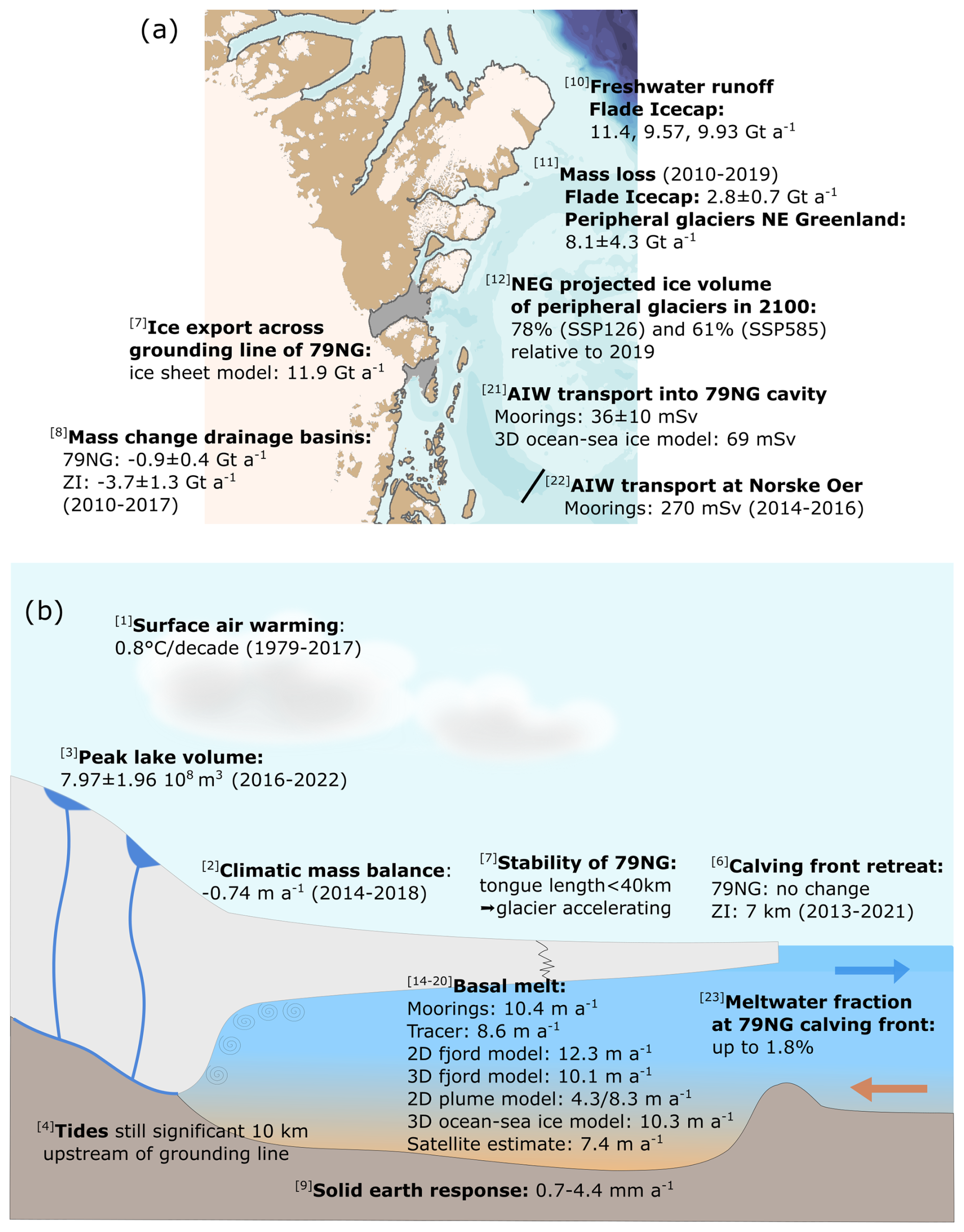
Figure 18Essence of mass-balance-related estimates of the GROCE project. Panel (a) shows the far-field estimates, while panel (b) displays the estimates related to 79NG. The numbers given in brackets preceding each entry refer to the corresponding entry in Table 1, which gives more detailed information. NEG: northeast Greenland.
Our estimates reveal that the recent mass loss of FIIC (2010–2019) amounts to as much as 70 % of the ZI (2010–2017) value. Regarding the annual freshwater runoff from FIIC, our estimates range between 9.6 and 11.4 Gt a−1, with 9.9 Gt a−1 being the best guess; in this regard, the high-resolution (NEGIS_WRF) forcing data improved the calibration of mass balance without requiring additional corrections. Based on our future projections, a considerable increase in mass loss from the peripheral glaciers of NE Greenland is anticipated by the end of the 21st century relative to the mass in 2019. The mass loss will likely contribute to a sea-level rise between 4 and 8 mm, contingent upon the specific emission scenarios. Recent investigations reveal that the mass loss from peripheral glaciers in north Greenland has exceeded that of the combined total of all other regions in Greenland over the past several decades (Khan et al., 2022b). It is projected that, in the future, the NE region will maintain its status as the predominant contributor to the total liquid freshwater, solid-ice calving and sea-level rise among Greenland's peripheral glaciers (Shafeeque et al., 2024). At the same time, the projected increasing freshwater flux by NE Greenland peripheral glaciers alone is unlikely to affect the strength of the Atlantic thermohaline circulation in a significant way within this century.
Basal melt rates of 79NG – another primary focus of the GROCE project – were derived from observational and numerical modeling approaches. Our observations from a year-long mooring-based time series of ocean heat transport allowed us to estimate the mean basal melt rate to be 10.4 ± 3.1 m a−1, while the observed tracer-based approach yielded 8.6 ± 1.4 m a−1. These two values represent bulk estimates of the melt rates (representing spatial average values for the whole ice tongue). In contrast, the radar-based measurements provide a spatial distribution with enhanced basal melt rates close to the grounding line – representing the zone of highest melt. Both the area-averaged estimates and point estimates can be reconciled with satellite-based estimates of the basal melt rate by Wilson et al. (2017). Their bulk estimate gives values of 7.4 m a−1, with maximum melt rates exceeding 50 m a−1 near the grounding line. It is likely that the Wilson approach underestimates the bulk rate because the underlying method does not resolve the extreme melt rates near the grounding zone revealed by Zeising et al. (2024a). Our modeling-based estimates show a remarkable agreement with the mooring-based results. In their basic configurations, with ocean temperatures close to the observed ones, the area-averaged annual mean melt rates are 12.3, 8.3, 10.1 and 10.3 m a−1 for the 2D fjord, 2D plume (rough ice base), 3D fjord and 3D ocean–sea ice model simulations, respectively. The tracer-observation-based estimate of the melt rate of 8.6 m a−1 was conducted during a time of particularly low AIW temperatures in summer 2016 that, according to Schaffer et al. (2020), were about 0.2–0.3 °C lower than the annual mean AIW temperature (August 2016–September 2017), which was used to derive the mooring-based estimate of 10.4 m a−1. Therefore, applying the simulated sensitivity of 0.64 m a−1 per 0.1 °C to the former estimate, an offset of 1.3–1.9 m a−1 would be applicable to account for the temperature difference, bringing both estimates in even closer agreement with each other.
Both the 2D fjord model and the 3D ocean model were used to explore melt rate sensitivities, displaying an above-linear dependency on ocean temperature change and a square-root relationship to subglacial discharge which also appear to hold for other floating ice tongue glaciers in north Greenland. Studies on Antarctic ice shelves have demonstrated the importance of subglacial discharge for the formation of basal channels at specific locations (e.g., Le Brocq et al., 2013; Wei et al., 2020), similar to our findings with the plume model. However, the net effect of subglacial discharge on area mean melt rates has been found to be small (5.7 % relative to a situation with zero discharge) for realistic discharge rates for Pine Island Glacier (PIG), Antarctica (Nakayama et al., 2021). This discrepancy can be attributed to the fact that total runoff fluxes are much smaller for Antarctica than for Greenland, e.g., 1.7 Gt a−1 for PIG (Nakayama et al., 2021) vs. about 5 Gt a−1 for the smaller 79NG (this study). Despite the difference in the absolute magnitude of the discharge, the square-root relationship that we find here is roughly consistent – though with a different offset – with results from the model experiments of Nakayama et al. (2021). PIG may actually serve as a suitable Antarctic parallel to 79NG: it is relatively small, features high melt rates due to warm water in the cavity, shows a large throughput of ice and drains an overproportionally large area of an ice sheet. Observation-based estimates of subglacial discharge (given as a fraction of the sum of basal melt and discharge; see Table 1) have been provided from the mooring data, yielding 11 %. This is in reasonable agreement with results from the 3D fjord and 3D ocean–sea ice models (11 % and 20 %, respectively), where the absolute value of discharge is prescribed (using a constant or time-variable flux).
In terms of ocean and subglacial fluxes inferred from the mooring-based observations, we find a transport of 270 mSv of AIW flowing toward the inner continental shelf, of which 36 mSv enters the cavity, resulting in a meltwater flux of 0.56 mSv (which is 2 orders of magnitudes smaller than the AIW inflow volume transport), supported by a subglacial discharge of 0.07 mSv. On the continental shelf, we find that the meltwater flowing out of the cavity of 79NG mostly stays within a depth range of 100–200 m. This is consistent with the meltwater plume detaching from the ice base before leaving the cavity – thus with detrainment of waters from the plume taking place – something which the idealized 2D fjord model actually shows. Once leaving the cavity, the meltwater quickly dilutes to values below the detection limit on the outer shelf, meaning that the subglacial-meltwater impact on the ocean stratification is limited to the near-coastal areas. Finally, looking on an east-Greenland-wide scale, the simulated near-shore sensitivity of the sea surface salinity to surface meltwater runoff (treating all meltwater as surface runoff) exceeds 0.5 g kg−1 (compared to a case where runoff is switched off), with the signal again quickly dissolving away from the coast the shelf edge. Thus we expect the anomaly to drive an anomalous, narrow along-coast circulation, which may impact the exchange of water between the fjords and the open ocean. On the western coast of Greenland, the surface freshwater anomaly extends far offshore (e.g., into Baffin Bay) and is associated with surface warming. Interestingly, Oltmanns et al. (2020) found that the strengthening of the ocean stratification was associated with increased freshwater runoff from Greenland causing the ocean surface temperature to rise above freezing earlier within the season and affecting air–sea heat fluxes and thus mid-latitude weather patterns significantly.
In the future, a more realistic treatment of meltwater runoff in model simulations would be desirable all around Greenland, in the sense that firstly it should be injected into the fjords at the correct depth levels (glacier base rather than surface) and secondly the meltwater signature of icebergs melting offshore should be taken into account (Moon et al., 2018). We assume that this treatment, by spreading the meltwater signature both in the vertical and horizontal domains, might largely change the simulated ocean circulation response to meltwater and ice discharge. As the submarine melt rate is strongly impacted by the prevailing ocean circulation, a more realistic approach of meltwater injection could possibly even feed back onto ocean-driven glacier melt (Davison et al., 2020). Last but not least, a seamless approach of linking the surface mass balance to the subglacial discharge via hydrological modeling would be desirable in order to use this as a temporally and spatially varying boundary condition for simulations of the ocean circulation and basal melt rate in the cavity of 79NG.
To conclude, the different in situ and remote sensing observations and model simulations together reveal a consistent picture of a coupled atmosphere–ice sheet–ocean system that responds to the changing climatic conditions and whose components have clearly evolved in the past decades.
The core datasets compiled in the framework of the GROCE project and forming the basis of this paper are provided here, referencing either the corresponding figure or value in Table 1. Respective publications are also included here.
Turton et al. (2020)Turton (2019)Blau et al. (2021)Turton et al. (2021b)Lutz et al. (2024a)Lutz et al. (2024b)Loebel et al. (2023, 2024)Humbert et al. (2023)Larour et al. (2012)Morlighem et al. (2017)Kappelsberger et al. (2021)(Kappelsberger et al., 2020)Kappelsberger et al. (2021)(Kappelsberger et al., 2021)Shafeeque and Marzeion (2024)McPherson et al. (2024)Schaffer and Kanzow (2019)McPherson and Kanzow (2024)Kanzow et al. (2017a)Kanzow et al. (2018)Zeising et al. (2024a)Zeising et al. (2024b, c)Mohammadi-Aragh and Burchard (2024)Reinert et al. (2023)Reinert (2023b)Wekerle et al. (2024)Wekerle (2023)Huhn et al. (2021a, b)Kanzow et al. (2017a, b)Stolzenberger et al. (2022)Stolzenberger (2022)Schaffer et al. (2020)von Appen et al. (2017a)Schaffer et al. (2019b)von Appen et al. (2017b)Schaffer et al. (2019c)Table A1Current data availability. Datasets used for each figure and corresponding quantity in Table 1, with respective publications. The table references both the scientific publications and the publications of the datasets.
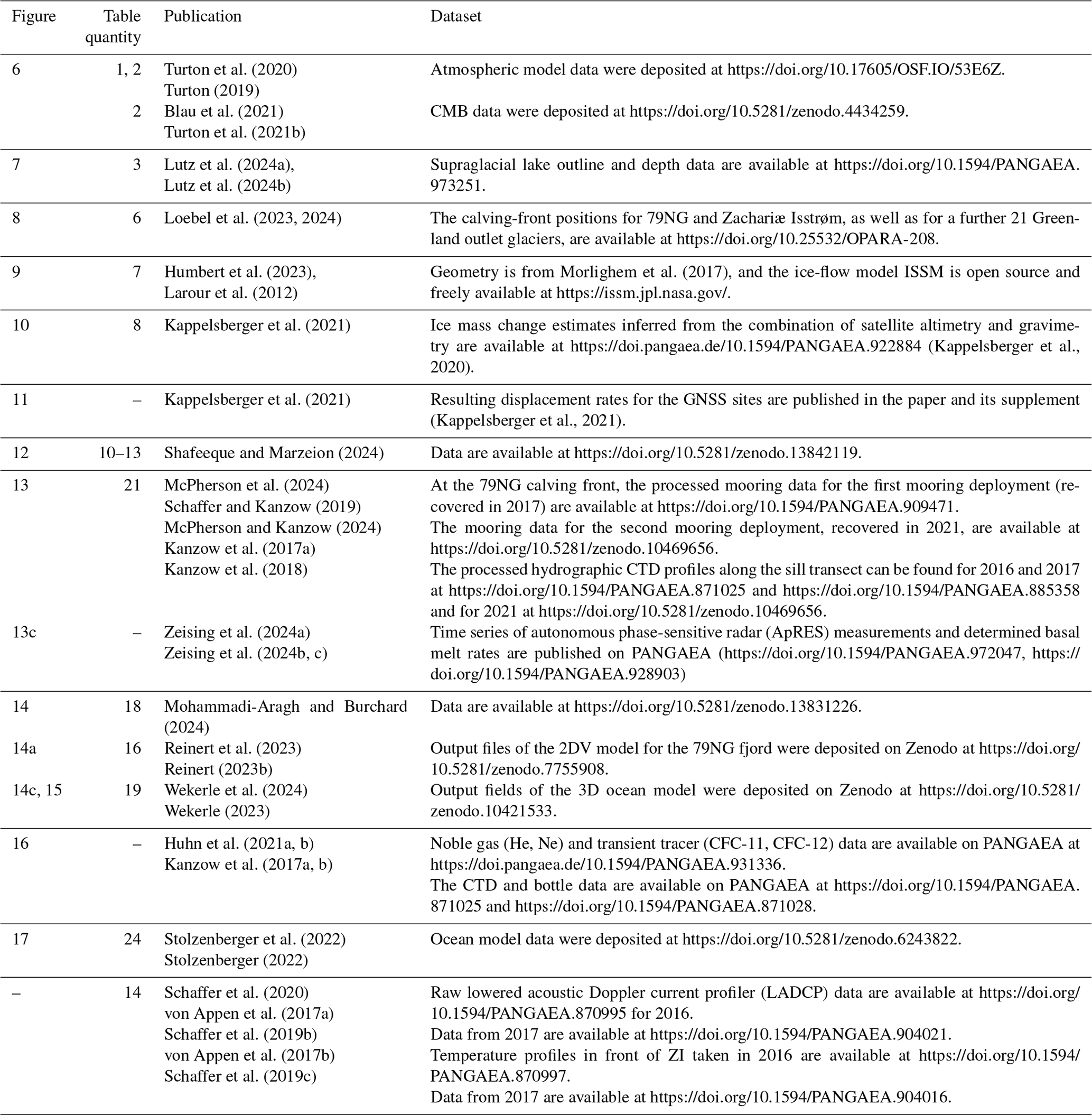
The codes used to create the figures and calculations can be obtained from the authors upon request. The code of the idealized 2D fjord model for 79NG can be downloaded from https://doi.org/10.5281/zenodo.7741925 (Klingbeil, 2023) and https://doi.org/10.5281/zenodo.7755753 (Reinert, 2023a). The code of the plume model GIPM is available at https://doi.org/10.5281/zenodo.13831226 (Mohammadi-Aragh and Burchard, 2024).
The data sources of most of the datasets forming the basis of this paper are given in the references provided throughout the text and are summarized in the data appendix in Table A1.
All authors contributed to the writing and data analysis. TK, TM, MS and AH coordinated the writing process.
At least one of the (co-)authors is a member of the editorial board of The Cryosphere. The peer-review process was guided by an independent editor, and the authors also have no other competing interests to declare.
Publisher’s note: Copernicus Publications remains neutral with regard to jurisdictional claims made in the text, published maps, institutional affiliations, or any other geographical representation in this paper. While Copernicus Publications makes every effort to include appropriate place names, the final responsibility lies with the authors.
The authors would like to acknowledge the support provided by the German Federal Ministry for Education and Research (BMBF) within the projects GROCE from 2016–2019 and GROCE 2 from 2020–2024. This funding provided the decisive basis to accomplish this study. The authors would like to express their gratitude to the Projektträger Jülich (PTJ) for continuous support and interest during the execution of the GROCE and GROCE 2 projects. The research work was also supported by the Deutsche Forschungsgemeinschaft (DFG) Special Priority Program (SPP) 1889 “Regional Sea Level Change and Society” (SeaLevel), as well as by the Helmholtz Society (Impulse and Network Fund). The authors gratefully acknowledge the computing time granted by the Resource Allocation Board for the supercomputer Lise at NHR@ZIB (National High Performance Computing at the Zuse Institute Berlin) as part of the NHR infrastructure. We thank the captains and crews of RV Polarstern (Alfred-Wegener-Institut Helmholtz-Zentrum für Polar- und Meeresforschung, 2017), the helicopter crews and the German weather forecasters for their great support of our measurements at 79NG and ZI during expeditions PS100 (2016) and PS109 (2017). Ship time was provided under grants AWI_PS100_01, AWI_PS109_03 and AWI_PS114_01. We thank the captain and entire crew of HDMS Triton and the Danish Arctic Command for their support in recovering the moorings at 79NG in 2021. The authors would like to express their deep gratitude to the three reviewers, whose comments helped to improve the manuscript in many ways.
This research has been supported by the German Federal Ministry for Education and Research (grant nos. 03F0778 and 03F0855) and the Deutsche Forschungsgemeinschaft (grant no. KA 3204/5).
The article processing charges for this open-access publication were covered by the Alfred-Wegener-Institut Helmholtz-Zentrum für Polar- und Meeresforschung.
This paper was edited by Kerim Nisancioglu and reviewed by Shfaqat Abbas Khan and two anonymous referees.
A, G., Wahr, J., and Zhong, S.: Computations of the viscoelastic response of a 3-D compressible Earth to surface loading: an application to Glacial Isostatic Adjustment in Antarctica and Canada, Geophys. J. Int., 192, 557–572, https://doi.org/10.1093/gji/ggs030, 2012. a
Alfred-Wegener-Institut Helmholtz-Zentrum für Polar- und Meeresforschung: Polar Research and Supply Vessel POLARSTERN Operated by the Alfred-Wegener-Institute, Journal of Large-Scale Research Facilities, 3, A119, https://doi.org/10.17815/jlsrf-3-163, 2017. a
Aschwanden, A., Fahnestock, M. A., and Truffer, M.: Complex Greenland outlet glacier flow captured, Nat. Commun., 7, 10524, https://doi.org/10.1038/ncomms10524, 2016. a
Bamber, J. L., Tedstone, A. J., King, M. D., Howat, I. M., Enderlin, E. M., van den Broeke, M. R., and Noel, B.: Land Ice Freshwater Budget of the Arctic and North Atlantic Oceans: 1. Data, Methods, and Results, J. Geophys. Res.-Oceans, 123, 1827–1837, https://doi.org/10.1002/2017jc013605, 2018. a, b
Beszczynska-Möller, A., Fahrbach, E., Schauer, U., and Hansen, E.: Variability in Atlantic water temperature and transport at the entrance to the Arctic Ocean, 1997–2010, ICES J. Mar. Sci., 69, 852–863, https://doi.org/10.1093/icesjms/fss056, 2012. a
Bettadpur, S.: CSR Level-2 processing standards document for product release 06, GRACE 327–742, Revision 5.0, https://podaac.jpl.nasa.gov/gravity/grace-documentation (last access: 10 April 2025), 2018. a
Bevis, M., Harig, C., Khan, S. A., Brown, A., Simons, F. J., Willis, M., Fettweis, X., van den Broeke, M. R., Madsen, F. B., Kendrick, E., Caccamise, D. J., van Dam, T., Knudsen, P., and Nylen, T.: Accelerating changes in ice mass within Greenland, and the ice sheet’s sensitivity to atmospheric forcing, P. Natl. Acad. Sci. USA, 116, 1934–1939, https://doi.org/10.1073/pnas.1806562116, 2019. a
Beyer, S., Kleiner, T., Aizinger, V., Rückamp, M., and Humbert, A.: A confined–unconfined aquifer model for subglacial hydrology and its application to the Northeast Greenland Ice Stream, The Cryosphere, 12, 3931–3947, https://doi.org/10.5194/tc-12-3931-2018, 2018. a, b
Blau, M. T., Turton, J. V., Sauter, T., and Mölg, T.: Surface mass balance and energy balance of the 79N Glacier (Nioghalvfjerdsfjorden, NE Greenland) modeled by linking COSIPY and Polar WRF, J. Glaciol., 67, 1093–1107, https://doi.org/10.1017/jog.2021.56, 2021. a, b, c, d, e
Bolch, T., Sandberg Sørensen, L., Simonsen, S. B., Mölg, N., Machguth, H., Rastner, P., and Paul, F.: Mass loss of Greenland’s glaciers and ice caps 2003–2008 revealed from ICESat laser altimetry data, Geophys. Res. Lett., 40, 875–881, https://doi.org/10.1002/grl.50270, 2013. a
Bollen, K. E., Enderlin, E. M., and Muhlheim, R.: Dynamic mass loss from Greenland’s marine-terminating peripheral glaciers (1985–2018), J. Glaciol., 69, 153–163, https://doi.org/10.1017/jog.2022.52, 2022. a
Böning, C. W., Behrens, E., Biastoch, A., Getzlaff, K., and Bamber, J. L.: Emerging impact of Greenland meltwater on deepwater formation in the North Atlantic Ocean, Nat. Geosci., 9, 523–527, 2016. a, b
Brunnabend, S., Schröter, J., Rietbroek, R., and Kusche, J.: Regional sea level change in response to ice mass loss in Greenland, the West Antarctic and Alaska, J. Geophys. Res.-Oceans, 120, 7316–7328, https://doi.org/10.1002/2015jc011244, 2015. a
Budd, W. F., Jenssen, D., and Smith, I. N.: A Three-Dimensional Time-Dependent Model of the West Antarctic Ice Sheet, Ann. Glaciol., 5, 29–36, https://doi.org/10.3189/1984aog5-1-29-36, 1984. a
Burchard, H. and Bolding, K.: GETM, a general estuarine transport model, technical report no. EUR 20253 EN, https://publications.jrc.ec.europa.eu/repository/handle/JRC23237 (last access: 20 March 2025), 2022. a
Burchard, H., Bolding, K., Jenkins, A., Losch, M., Reinert, M., and Umlauf, L.: The Vertical Structure and Entrainment of Subglacial Melt Water Plumes, J. Adv. Model. Earth Sy., 14, e2021MS002925, https://doi.org/10.1029/2021ms002925, 2022. a
Cai, C., Rignot, E., Menemenlis, D., and Nakayama, Y.: Observations and modeling of ocean-induced melt beneath Petermann Glacier Ice Shelf in northwestern Greenland, Geophys. Res. Lett., 44, 8396–8403, https://doi.org/10.1002/2017GL073711, 2017. a
Caron, L., Ivins, E. R., Larour, E., Adhikari, S., Nilsson, J., and Blewitt, G.: GIA Model Statistics for GRACE Hydrology, Cryosphere, and Ocean Science, Geophys. Res. Lett., 45, 2203–2212, https://doi.org/10.1002/2017gl076644, 2018. a, b, c
Chafik, L., Nilsen, J. E. O., Dangendorf, S., Reverdin, G., and Frederikse, T.: North Atlantic Ocean Circulation and Decadal Sea Level Change During the Altimetry Era, Scientific Reports, 9, 1041, https://doi.org/10.1038/s41598-018-37603-6, 2019. a
Christmann, J., Helm, V., Khan, S. A., Kleiner, T., Müller, R., Morlighem, M., Neckel, N., Rückamp, M., Steinhage, D., Zeising, O., and Humbert, A.: Elastic deformation plays a non-negligible role in Greenland’s outlet glacier flow, Communications Earth & Environment, 2, 232, https://doi.org/10.1038/s43247-021-00296-3, 2021. a, b, c
Copernicus Climate Change Service: ERA5-Land hourly data from 1950 to present, Copernicus Climate Change Service [data set], https://doi.org/10.24381/CDS.E2161BAC, 2019. a
Davison, B. J., Cowton, T. R., Cottier, F. R., and Sole, A. J.: Iceberg melting substantially modifies oceanic heat flux towards a major Greenlandic tidewater glacier, Nat. Commun., 11, 5983, https://doi.org/10.1038/s41467-020-19805-7, 2020. a
Dee, D. P., Uppala, S. M., Simmons, A. J., Berrisford, P., Poli, P., Kobayashi, S., Andrae, U., Balmaseda, M. A., Balsamo, G., Bauer, P., Bechtold, P., Beljaars, A. C. M., van de Berg, L., Bidlot, J., Bormann, N., Delsol, C., Dragani, R., Fuentes, M., Geer, A. J., Haimberger, L., Healy, S. B., Hersbach, H., Hólm, E. V., Isaksen, L., Kållberg, P., Köhler, M., Matricardi, M., McNally, A. P., Monge‐Sanz, B. M., Morcrette, J., Park, B., Peubey, C., de Rosnay, P., Tavolato, C., Thépaut, J., and Vitart, F.: The ERA‐Interim reanalysis: configuration and performance of the data assimilation system, Q. J. Roy. Meteor. Soc., 137, 553–597, https://doi.org/10.1002/qj.828, 2011. a
Edwards, T. L., Nowicki, S., Marzeion, B., Hock, R., Goelzer, H., Seroussi, H., Jourdain, N. C., Slater, D. A., Turner, F. E., Smith, C. J., McKenna, C. M., Simon, E., Abe-Ouchi, A., Gregory, J. M., Larour, E., Lipscomb, W. H., Payne, A. J., Shepherd, A., Agosta, C., Alexander, P., Albrecht, T., Anderson, B., Asay-Davis, X., Aschwanden, A., Barthel, A., Bliss, A., Calov, R., Chambers, C., Champollion, N., Choi, Y., Cullather, R., Cuzzone, J., Dumas, C., Felikson, D., Fettweis, X., Fujita, K., Galton-Fenzi, B. K., Gladstone, R., Golledge, N. R., Greve, R., Hattermann, T., Hoffman, M. J., Humbert, A., Huss, M., Huybrechts, P., Immerzeel, W., Kleiner, T., Kraaijenbrink, P., Le clec’h, S., Lee, V., Leguy, G. R., Little, C. M., Lowry, D. P., Malles, J.-H., Martin, D. F., Maussion, F., Morlighem, M., O’Neill, J. F., Nias, I., Pattyn, F., Pelle, T., Price, S. F., Quiquet, A., Radić, V., Reese, R., Rounce, D. R., Rückamp, M., Sakai, A., Shafer, C., Schlegel, N.-J., Shannon, S., Smith, R. S., Straneo, F., Sun, S., Tarasov, L., Trusel, L. D., Van Breedam, J., van de Wal, R., van den Broeke, M., Winkelmann, R., Zekollari, H., Zhao, C., Zhang, T., and Zwinger, T.: Projected land ice contributions to twenty-first-century sea level rise, Nature, 593, 74–82, https://doi.org/10.1038/s41586-021-03302-y, 2021. a
Enderlin, E. M. and Howat, I. M.: Submarine melt rate estimates for floating termini of Greenland outlet glaciers (2000–2010), J. Glaciol., 59, 67–75, https://doi.org/10.3189/2013jog12j049, 2013. a
Fichefet, T., Poncin, C., Goosse, H., Huybrechts, P., Janssens, I., and Le Treut, H.: Implications of changes in freshwater flux from the Greenland ice sheet for the climate of the 21st century, Geophys. Res. Lett., 30, 1911, https://doi.org/10.1029/2003gl017826, 2003. a
Gardner, A., Fahnestock, M., and Scambos, T.: MEASURES ITS LIVE Regional Glacier and Ice Sheet Surface Velocities, Version 1, NASA National Snow and Ice Data Center Distributed Active Archive Center [data set], https://doi.org/10.5067/6II6VW8LLWJ7, 2022. a
Gräwe, U., Holtermann, P., Klingbeil, K., and Burchard, H.: Advantages of vertically adaptive coordinates in numerical models of stratified shelf seas, Ocean Model., 92, 56–68, https://doi.org/10.1016/j.ocemod.2015.05.008, 2015. a
Groh, A. and Horwath, M.: Antarctic Ice Mass Change Products from GRACE/GRACE-FO Using Tailored Sensitivity Kernels, Remote Sensing, 13, 1736, https://doi.org/10.3390/rs13091736, 2021. a
Groh, A., Ewert, H., Fritsche, M., Rülke, A., Rosenau, R., Scheinert, M., and Dietrich, R.: Assessing the Current Evolution of the Greenland Ice Sheet by Means of Satellite and Ground-Based Observations, Surv. Geophys., 35, 1459–1480, https://doi.org/10.1007/s10712-014-9287-x, 2014. a
Harris, I., Osborn, T. J., Jones, P., and Lister, D.: Version 4 of the CRU TS monthly high-resolution gridded multivariate climate dataset, Scientific Data, 7, 109, https://doi.org/10.1038/s41597-020-0453-3, 2020. a
Hellmer, H. and Olbers, D.: A two-dimensional model for the thermohaline circulation under an ice shelf, Antarctic Science, 1, 325–336, https://doi.org/10.1017/S0954102089000490, 1989. a
Helm, V., Humbert, A., and Miller, H.: Elevation and elevation change of Greenland and Antarctica derived from CryoSat-2, The Cryosphere, 8, 1539–1559, https://doi.org/10.5194/tc-8-1539-2014, 2014. a, b, c
Henson, H., Holding, J., Meire, L., Rysgaard, S., Stedmon, C., Stuart-Lee, A., Bendtsen, J., and Sejr, M.: Coastal Freshening Drives Acidification State in Greenland Fjords, SSRN Electronic Journal, https://doi.org/10.2139/ssrn.4202079, 2022. a
Hines, K. M., Bromwich, D. H., Bai, L.-S., Barlage, M., and Slater, A. G.: Development and Testing of Polar WRF. Part III: Arctic Land, J. Climate, 24, 26–48, https://doi.org/10.1175/2010JCLI3460.1, 2011. a
Hochreuther, P., Neckel, N., Reimann, N., Humbert, A., and Braun, M.: Fully Automated Detection of Supraglacial Lake Area for Northeast Greenland Using Sentinel-2 Time-Series, Remote Sensing, 13, 205, https://doi.org/10.3390/rs13020205, 2021. a, b
Hofmeister, R., Burchard, H., and Beckers, J.-M.: Non-uniform adaptive vertical grids for 3D numerical ocean models, Ocean Model., 33, 70–86, https://doi.org/10.1016/j.ocemod.2009.12.003, 2010. a, b, c
Hofmeister, R., Beckers, J.-M., and Burchard, H.: Realistic modelling of the exceptional inflows into the central Baltic Sea in 2003 using terrain-following coordinates, Ocean Model., 39, 233–247, https://doi.org/10.1016/j.ocemod.2011.04.007, 2011. a
Højmark Thomsen, H., Reeh, N., Olesen, O. B., Egede Bøggilde, C., Starzer, W., Weidick, A., and Higgins, A. K.: The Nioghalvfjerdsfjorden glacier project, North-East Greenland: a study of ice sheet response to climatic change, Geology of Greenland Survey Bulletin, 176, 95–103, https://doi.org/10.34194/ggub.v176.5073, 1997. a
Hopwood, M. J., Carroll, D., Dunse, T., Hodson, A., Holding, J. M., Iriarte, J. L., Ribeiro, S., Achterberg, E. P., Cantoni, C., Carlson, D. F., Chierici, M., Clarke, J. S., Cozzi, S., Fransson, A., Juul-Pedersen, T., Winding, M. H. S., and Meire, L.: Review article: How does glacier discharge affect marine biogeochemistry and primary production in the Arctic?, The Cryosphere, 14, 1347–1383, https://doi.org/10.5194/tc-14-1347-2020, 2020. a
Hörhold, M., Münch, T., Weißbach, S., Kipfstuhl, S., Freitag, J., Sasgen, I., Lohmann, G., Vinther, B., and Laepple, T.: Modern temperatures in central–north Greenland warmest in past millennium, Nature, 613, 503–507, https://doi.org/10.1038/s41586-022-05517-z, 2023. a
Horwath, M., Gutknecht, B. D., Cazenave, A., Palanisamy, H. K., Marti, F., Marzeion, B., Paul, F., Le Bris, R., Hogg, A. E., Otosaka, I., Shepherd, A., Döll, P., Cáceres, D., Müller Schmied, H., Johannessen, J. A., Nilsen, J. E. Ø., Raj, R. P., Forsberg, R., Sandberg Sørensen, L., Barletta, V. R., Simonsen, S. B., Knudsen, P., Andersen, O. B., Ranndal, H., Rose, S. K., Merchant, C. J., Macintosh, C. R., von Schuckmann, K., Novotny, K., Groh, A., Restano, M., and Benveniste, J.: Global sea-level budget and ocean-mass budget, with a focus on advanced data products and uncertainty characterisation, Earth Syst. Sci. Data, 14, 411–447, https://doi.org/10.5194/essd-14-411-2022, 2022. a
Howat, I. M., Joughin, I., Fahnestock, M., Smith, B. E., and Scambos, T. A.: Synchronous retreat and acceleration of southeast Greenland outlet glaciers 2000–06: ice dynamics and coupling to climate, J. Glaciol., 54, 646–660, https://doi.org/10.3189/002214308786570908, 2008. a
Hugonnet, R., McNabb, R., Berthier, E., Menounos, B., Nuth, C., Girod, L., Farinotti, D., Huss, M., Dussaillant, I., Brun, F., and Kääb, A.: Accelerated global glacier mass loss in the early twenty-first century, Nature, 592, 726–731, https://doi.org/10.1038/s41586-021-03436-z, 2021. a
Huhn, O., Rhein, M., Kanzow, T., Schaffer, J., and Sültenfuß, J.: Submarine Meltwater From Nioghalvfjerdsbræ (79 North Glacier), Northeast Greenland, J. Geophys. Res.-Oceans, 126, e2021JC017224, https://doi.org/10.1029/2021JC017224, 2021a. a, b, c, d, e, f
Huhn, O., Rhein, M., Bulsiewicz, K., and Sültenfuß, J.: Noble gas (He, Ne isotopes) and transient tracer (CFC-11 and CFC-12) measurements from POLARSTERN cruise PS100 (northeast Greenland, 2016), PANGAEA [data set], https://doi.org/10.1594/PANGAEA.931336, 2021b. a
Humbert, A., Helm, V., Neckel, N., Zeising, O., Rückamp, M., Khan, S. A., Loebel, E., Brauchle, J., Stebner, K., Gross, D., Sondershaus, R., and Müller, R.: Precursor of disintegration of Greenland's largest floating ice tongue, The Cryosphere, 17, 2851–2870, https://doi.org/10.5194/tc-17-2851-2023, 2023. a, b, c, d
Huss, M. and Hock, R.: A new model for global glacier change and sea-level rise, Front. Earth Sci., 3, 54, https://doi.org/10.3389/feart.2015.00054, 2015. a
Jenkins, A., Shoosmith, D., Dutrieux, P., Jacobs, S., Kim, T. W., Lee, S. H., Ha, H. K., and Stammerjohn, S.: West Antarctic Ice Sheet retreat in the Amundsen Sea driven by decadal oceanic variability, Nat. Geosci., 11, 733–738, https://doi.org/10.1038/s41561-018-0207-4, 2018. a
Joughin, I.: MEaSUREs Greenland Ice Sheet Velocity Map from InSAR Data, Version 2, NASA National Snow and Ice Data Center Distributed Active Archive Center [data set], https://doi.org/10.5067/OC7B04ZM9G6Q, 2015. a, b
Joughin, I., Smith, B. E., Shean, D. E., and Floricioiu, D.: Brief Communication: Further summer speedup of Jakobshavn Isbræ, The Cryosphere, 8, 209–214, https://doi.org/10.5194/tc-8-209-2014, 2014. a
Kanzow, T.: The Expedition PS100 of the Research Vessel POLARSTERN to the Fram Strait in 2016, Tech. Rep., Alfred-Wegener-Institut, Helmholtz-Zentrum für Polar- und Meeresforschung, https://doi.org/10.2312/BZPM_0705_2017, 2017. a, b
Kanzow, T.: The Expedition PS109 of the Research Vessel POLARSTERN to the Nordic Seas in 2017, Tech. rep., Alfred-Wegener-Institut, Helmholtz-Zentrum für Polar- und Meeresforschung, Bremerhaven, https://doi.org/10.2312/BzPM_0715_2018, 2018. a
Kanzow, T., von Appen, W.-J., Schaffer, J., Köhn, E., Tsubouchi, T., Wilson, N., and Wisotzki, A.: Physical oceanography measured with CTD/Large volume Watersampler-system during POLARSTERN cruise PS100 (ARK-XXX/2) [dataset]. Alfred Wegener Institute, Helmholtz Centre for Polar and Marine Research, Bremerhaven, PANGAEA [data set], https://doi.org/10.1594/PANGAEA.871025, 2017a. a, b
Kanzow, T., von Appen, W.-J., Schaffer, J., Köhn, E., Tsubouchi, T., Wilson, N., and Wisotzki, A.: Physical oceanography measured on water bottle samples from CTD/Large volume Watersampler-system during POLARSTERN cruise PS100 (ARK-XXX/2) [dataset]. Alfred Wegener Institute, Helmholtz Centre for Polar and Marine Research, Bremerhaven, PANGAEA, https://doi.org/10.1594/PANGAEA.871028, 2017b. a
Kanzow, T., Schaffer, J., and Rohardt, G.: Physical oceanography during POLARSTERN cruise PS109 (ARK-XXXI/4) [dataset]. Alfred Wegener Institute, Helmholtz Centre for Polar and Marine Research, Bremerhaven, PANGAEA [data set], https://doi.org/10.1594/PANGAEA.885358, 2018. a
Kappelsberger, M., Strößenreuther, U., Scheinert, M., Horwath, M., and Groh, A.: Gridded rates of ice-mass change in north-east Greenland from a combination of satellite gravimetry and satellite altimetry, PANGAEA [data set], https://doi.org/10.1594/PANGAEA.922884, 2020. a, b, c
Kappelsberger, M. T., Strößenreuther, U., Scheinert, M., Horwath, M., Groh, A., Knöfel, C., Lunz, S., and Khan, S. A.: Modeled and Observed Bedrock Displacements in North‐East Greenland Using Refined Estimates of Present‐Day Ice‐Mass Changes and Densified GNSS Measurements, J. Geophys. Res.-Earth, 126, e2020JF005860, https://doi.org/10.1029/2020JF005860, 2021. a, b, c, d, e, f, g, h, i, j, k, l, m, n, o, p, q, r, s, t
Khan, S. A., Kjær, K. H., Bevis, M., Bamber, J. L., Wahr, J., Kjeldsen, K. K., Bjørk, A. A., Korsgaard, N. J., Stearns, L. A., van den Broeke, M. R., Liu, L., Larsen, N. K., and Muresan, I. S.: Sustained mass loss of the northeast Greenland ice sheet triggered by regional warming, Nat. Clim. Change, 4, 292–299, https://doi.org/10.1038/nclimate2161, 2014. a
Khan, S. A., Aschwanden, A., Bjørk, A. A., Wahr, J., Kjeldsen, K. K., and Kjær, K. H.: Greenland ice sheet mass balance: a review, Reports on Progress in Physics, 78, 046801, https://doi.org/10.1088/0034-4885/78/4/046801, 2015. a
Khan, S. A., Sasgen, I., Bevis, M., Van Dam, T., Bamber, J. L., Wahr, J., Willis, M., Kjær, K. H., Wouters, B., Helm, V., Csatho, B., Fleming, K., Bjørk, A. A., Aschwanden, A., Knudsen, P., and Munneke, P. K.: Geodetic measurements reveal similarities between post–Last Glacial Maximum and present-day mass loss from the Greenland ice sheet, Science Advances, 2, e1600931, https://doi.org/10.1126/sciadv.1600931, 2016. a, b, c, d
Khan, S. A., Bamber, J. L., Rignot, E., Helm, V., Aschwanden, A., Holland, D. M., van den Broeke, M., King, M., Noël, B., Truffer, M., Humbert, A., Colgan, W., Vijay, S., and Kuipers Munneke, P.: Greenland Mass Trends From Airborne and Satellite Altimetry During 2011–2020, J. Geophys. Res.-Earth, 127, e2021JF006505, https://doi.org/10.1029/2021jf006505, 2022a. a
Khan, S. A., Colgan, W., Neumann, T. A., Van Den Broeke, M. R., Brunt, K. M., Noël, B., Bamber, J. L., Hassan, J., and Bjørk, A. A.: Accelerating Ice Loss From Peripheral Glaciers in North Greenland, Geophys. Res. Lett., 49, e2022GL098915, https://doi.org/10.1029/2022GL098915, 2022b. a, b, c, d
Khazendar, A., Fenty, I. G., Carroll, D., Gardner, A., Lee, C. M., Fukumori, I., Wang, O., Zhang, H., Seroussi, H., Moller, D., Noël, B. P. Y., Van Den Broeke, M. R., Dinardo, S., and Willis, J.: Interruption of two decades of Jakobshavn Isbrae acceleration and thinning as regional ocean cools, Nat. Geosci., 12, 277–283, https://doi.org/10.1038/s41561-019-0329-3, 2019. a
Kjeldsen, K., Korsgaard, N., Bjørk, A., Khan, S., Box, J., Funder, S., Larsen, N., Bamber, J., Colgan, W., Van Den Broeke, M., Siggaard-Andersen, M.-L., Nuth, C., Schomacker, A., Andresen, C., Willerslev, E., and Kjær, K.: Spatial and temporal distribution of mass loss from the Greenland Ice Sheet since AD 1900, Nature, 528, 396–400, https://doi.org/10.1038/nature16183, 2015. a
Klingbeil, K.: Source code for the coastal ocean model GETM (glacial_ice branch), Zenodo [code], https://doi.org/10.5281/zenodo.7741925, 2023. a
Krieger, L., Floricioiu, D., and Neckel, N.: Drainage basin delineation for outlet glaciers of Northeast Greenland based on Sentinel-1 ice velocities and TanDEM-X elevations, Remote Sens. Environ., 237, 111483, https://doi.org/10.1016/j.rse.2019.111483, 2020. a
Kvas, A., Behzadpour, S., Ellmer, M., Klinger, B., Strasser, S., Zehentner, N., and Mayer‐Gürr, T.: ITSG‐Grace2018: Overview and Evaluation of a New GRACE‐Only Gravity Field Time Series, J. Geophys. Res.-Sol. Ea., 124, 9332–9344, https://doi.org/10.1029/2019JB017415, 2019. a
Larour, E., Seroussi, H., Morlighem, M., and Rignot, E.: Continental scale, high order, high spatial resolution, ice sheet modeling using the Ice Sheet System Model (ISSM), J. Geophys. Res.-Earth, 117, 2011JF002140, https://doi.org/10.1029/2011JF002140, 2012 (code available at: https://issm.jpl.nasa.gov/, last access: 29 January 2025). a, b
Le Brocq, A., Ross, N., Griggs, J., Bingham, R., Corr, H., Ferraccioli, F., Jenkins, A., Jordan, T., Payne, A., Rippin, D., and Siegert, M.: Evidence from ice shelves for channelized meltwater flow beneath the Antarctic Ice Sheet, Nat. Geosci., 6, 945–948, https://doi.org/10.1038/ngeo1977, 2013. a
Lecavalier, B. S., Milne, G. A., Simpson, M. J., Wake, L., Huybrechts, P., Tarasov, L., Kjeldsen, K. K., Funder, S., Long, A. J., Woodroffe, S., Dyke, A. S., and Larsen, N. K.: A model of Greenland ice sheet deglaciation constrained by observations of relative sea level and ice extent, Quaternary Sci. Rev., 102, 54–84, https://doi.org/10.1016/j.quascirev.2014.07.018, 2014. a, b, c
Li, X., Lorenz, M., Klingbeil, K., Chrysagi, E., Gräwe, U., Wu, J., and Burchard, H.: Salinity Mixing and Diahaline Exchange Flow in a Large Multi-Outlet Estuary with Islands, J. Phys. Oceanogr., 52, 2111–2127, https://doi.org/10.1175/JPO-D-21-0292.1, 2022. a
Ligtenberg, S. R. M., Kuipers Munneke, P., Noël, B. P. Y., and van den Broeke, M. R.: Brief communication: Improved simulation of the present-day Greenland firn layer (1960–2016), The Cryosphere, 12, 1643–1649, https://doi.org/10.5194/tc-12-1643-2018, 2018. a
Lindeman, M. R., Straneo, F., Wilson, N. J., Toole, J. M., Krishfield, R. A., Beaird, N. L., Kanzow, T., and Schaffer, J.: Ocean Circulation and Variability Beneath Nioghalvfjerdsbræ (79 North Glacier) Ice Tongue, J. Geophys. Res.-Oceans, 125, e2020JC016091, https://doi.org/10.1029/2020JC016091, 2020. a
Löcher, A. and Kusche, J.: A hybrid approach for recovering high-resolution temporal gravity fields from satellite laser ranging, J. Geodesy, 95, 6, https://doi.org/10.1007/s00190-020-01460-x, 2021. a
Loebel, E., Scheinert, M., Horwath, M., Heidler, K., Christmann, J., Phan, L. D., Humbert, A., and Zhu, X. X.: Extracting Glacier Calving Fronts by Deep Learning: The Benefit of Multispectral, Topographic, and Textural Input Features, IEEE T. Geosci. Remote, 60, 4306112, https://doi.org/10.1109/TGRS.2022.3208454, 2022. a, b, c
Loebel, E., Scheinert, M., Horwath, M., Humbert, A., Sohn, J., Heidler, K., Liebezeit, C., and Zhu, X. X.: Data product of Greenland glacier calving front locations delineated by deep learning, 2013 to 2021, TU Dresden [data set], https://doi.org/10.25532/OPARA-208, 2023. a
Loebel, E., Scheinert, M., Horwath, M., Humbert, A., Sohn, J., Heidler, K., Liebezeit, C., and Zhu, X. X.: Calving front monitoring at a subseasonal resolution: a deep learning application for Greenland glaciers, The Cryosphere, 18, 3315–3332, https://doi.org/10.5194/tc-18-3315-2024, 2024. a, b, c, d
Loose, B. and Jenkins, W. J.: The five stable noble gases are sensitive unambiguous tracers of glacial meltwater, Geophys. Res. Lett., 41, 2835–2841, https://doi.org/10.1002/2013GL058804, 2014. a
Lozier, M. S.: Overturning in the subpolar North Atlantic: a review, Philos. T. Roy. Soc. A, 381, 20220191, https://doi.org/10.1098/rsta.2022.0191, 2023. a, b, c
Lutz, K., Bever, L., Sommer, C., Seehaus, T., Humbert, A., Scheinert, M., and Braun, M.: Assessing supraglacial lake depth using ICESat-2, Sentinel-2, TanDEM-X, and in situ sonar measurements over Northeast and Southwest Greenland, The Cryosphere, 18, 5431–5449, https://doi.org/10.5194/tc-18-5431-2024, 2024a. a, b
Lutz, K., Bahrami, Z., and Braun, M. H.: Supraglacial lake outlines over Northeast Greenland from 2016 to 2022 using deep learning methods based on Sentinel-2 imagery, PANGAEA [data set], https://doi.org/10.1594/PANGAEA.973251, 2024b. a
Malles, J.-H., Maussion, F., Ultee, L., Kochtitzky, W., Copland, L., and Marzeion, B.: Exploring the impact of a frontal ablation parameterization on projected 21st-century mass change for Northern Hemisphere glaciers, J. Glaciol., 69, 1317–1332, https://doi.org/10.1017/jog.2023.19, 2023. a
MacGregor, J. A., Fahnestock, M. A., Colgan, W. T., Larsen, N. K., Kjeldsen, K. K., and Welker, J. M.: The age of surface-exposed ice along the northern margin of the Greenland Ice Sheet, J. Glaciol., 66, 667–684, https://doi.org/10.1017/jog.2020.62, 2020.
Mankoff, K. D., Noël, B., Fettweis, X., Ahlstrøm, A. P., Colgan, W., Kondo, K., Langley, K., Sugiyama, S., van As, D., and Fausto, R. S.: Greenland liquid water discharge from 1958 through 2019, Earth Syst. Sci. Data, 12, 2811–2841, https://doi.org/10.5194/essd-12-2811-2020, 2020a. a, b
Mankoff, K. D., Solgaard, A., Colgan, W., Ahlstrøm, A. P., Khan, S. A., and Fausto, R. S.: Greenland Ice Sheet solid ice discharge from 1986 through March 2020, Earth Syst. Sci. Data, 12, 1367–1383, https://doi.org/10.5194/essd-12-1367-2020, 2020b. a, b
Mankoff, K. D., Fettweis, X., Langen, P. L., Stendel, M., Kjeldsen, K. K., Karlsson, N. B., Noël, B., van den Broeke, M. R., Solgaard, A., Colgan, W., Box, J. E., Simonsen, S. B., King, M. D., Ahlstrøm, A. P., Andersen, S. B., and Fausto, R. S.: Greenland ice sheet mass balance from 1840 through next week, Earth Syst. Sci. Data, 13, 5001–5025, https://doi.org/10.5194/essd-13-5001-2021, 2021. a
Maraun, D.: Bias Correcting Climate Change Simulations – a Critical Review, Current Climate Change Reports, 2, 211–220, https://doi.org/10.1007/s40641-016-0050-x, 2016. a
Martin, T., Biastoch, A., Lohmann, G., Mikolajewicz, U., and Wang, X.: On Timescales and Reversibility of the Ocean's Response to Enhanced Greenland Ice Sheet Melting in Comprehensive Climate Models, Geophys. Res. Lett., 49, e2021GL097114, https://doi.org/10.1029/2021GL097114, 2022. a, b
Maussion, F., Butenko, A., Champollion, N., Dusch, M., Eis, J., Fourteau, K., Gregor, P., Jarosch, A. H., Landmann, J., Oesterle, F., Recinos, B., Rothenpieler, T., Vlug, A., Wild, C. T., and Marzeion, B.: The Open Global Glacier Model (OGGM) v1.1, Geosci. Model Dev., 12, 909–931, https://doi.org/10.5194/gmd-12-909-2019, 2019. a
Mayer, C., Reeh, N., Jung‐Rothenhäusler, F., Huybrechts, P., and Oerter, H.: The subglacial cavity and implied dynamics under Nioghalvfjerdsfjorden Glacier, NE‐Greenland, Geophys. Res. Lett., 27, 2289–2292, https://doi.org/10.1029/2000GL011514, 2000. a
Mayer, C., Schaffer, J., Hattermann, T., Floricioiu, D., Krieger, L., Dodd, P. A., Kanzow, T., Licciulli, C., and Schannwell, C.: Large ice loss variability at Nioghalvfjerdsfjorden Glacier, Northeast-Greenland, Nat. Commun., 9, 2768, https://doi.org/10.1038/s41467-018-05180-x, 2018. a, b, c, d, e
McPherson, R. and Kanzow, T.: Mooring and CTD data at the 79NG calving front, Zenodo [data set], https://doi.org/10.5281/zenodo.10469656, 2024. a
McPherson, R. A., Engicht, C., and Kanzow, T.: The Expedition TRITON2021 of Hendes Dansk Majestæt Skib TRITON to the Greenland Sea in 2021, Tech. Rep., Bremerhaven, https://doi.org/10.57738/BzPM_0769_2023, 2023a. a
McPherson, R. A., Wekerle, C., and Kanzow, T.: Shifts of the Recirculation Pathways in Central Fram Strait Drive Atlantic Intermediate Water Variability on Northeast Greenland Shelf, J. Geophys. Res.-Oceans, 128, e2023JC019915, https://doi.org/10.1029/2023JC019915, 2023b. a, b, c, d, e
McPherson, R. A., Wekerle, C., Kanzow, T., Ionita, M., Heukamp, F. O., Zeising, O., and Humbert, A.: Atmospheric blocking slows ocean-driven melting of Greenland’s largest glacier tongue, Science, 385, 1360–1366, https://doi.org/10.1126/science.ado5008, 2024. a, b, c, d, e, f, g
Meredith, M., Sommerkorn, M., Cassotta, S., Derksen, C., Ekaykin, A., Hollowed, A., Kofinas, G., Mackintosh, A., Melbourne-Thomas, J., Muelbert, M., Ottersen, G., Pritchard, H., and Schuur, E.: Polar Regions, in: IPCC Special Report on the Ocean and Cryosphere in a Changing Climate, Cambridge University Press, 203–320, ISBN 9781009157971, https://doi.org/10.1017/9781009157964.005, 2019. a, b
Mertens, C., Huhn, O., Rapp, I., Benz, F., Stiehler, J., Bastian, D., Filella, A., Unger-Moreno, K., Bornemann, J., Böckmann, L., Böke, W., Chercham, C., Fiedler, G., Heinicke, J. R., Hinse, Y., Kalvelage, T., Kirchner, J., Lauber, J., Mirau, B., Purcel, K., and Sukhikh, N.: Greenland melt water in the western Nordic Seas and the Irminger Sea, Cruise No. MSM85, July 23 - August 13, 2019, St. John's (Canada) – Longyearbyen (Norway), Tech. Rep., Gutachterpanel Forschungsschiffe, https://doi.org/10.48433/CR_MSM85, 2020. a
Milne, G. A., Gehrels, W. R., Hughes, C. W., and Tamisiea, M. E.: Identifying the causes of sea-level change, Nat. Geosci., 2, 471–478, https://doi.org/10.1038/ngeo544, 2009. a
Mohammadi-Aragh, M. and Burchard, H.: Source code for the General Ice shelf water Plume Model (GIPM), Zenodo [code], https://doi.org/10.5281/zenodo.13831226, 2024. a, b, c
Mölg, T. and Kaser, G.: A new approach to resolving climate-cryosphere relations: Downscaling climate dynamics to glacier-scale mass and energy balance without statistical scale linking, J. Geophys. Res., 116, D16101, https://doi.org/10.1029/2011JD015669, 2011. a
Möller, M., Friedl, P., Palmer, S. J., and Marzeion, B.: Grounding Line Retreat and Ice Discharge Variability at Two Surging, Ice Shelf‐Forming Basins of Flade Isblink Ice Cap, Northern Greenland, J. Geophys. Res.-Earth, 127, e2021JF006302, https://doi.org/10.1029/2021JF006302, 2022. a, b, c
Moon, T., Joughin, I., Smith, B., and Howat, I.: 21st-Century Evolution of Greenland Outlet Glacier Velocities, Science, 336, 576–578, https://doi.org/10.1126/science.1219985, 2012. a
Moon, T., Sutherland, D. A., Carroll, D., Felikson, D., Kehrl, L., and Straneo, F.: Subsurface iceberg melt key to Greenland fjord freshwater budget, Nat. Geosci., 11, 49–54, https://doi.org/10.1038/s41561-017-0018-z, 2018. a
Morlighem, M., Williams, C. N., Rignot, E., An, L., Arndt, J. E., Bamber, J. L., Catania, G., Chauché, N., Dowdeswell, J. A., Dorschel, B., Fenty, I., Hogan, K., Howat, I., Hubbard, A., Jakobsson, M., Jordan, T. M., Kjeldsen, K. K., Millan, R., Mayer, L., Mouginot, J., Noël, B. P. Y., O'Cofaigh, C., Palmer, S., Rysgaard, S., Seroussi, H., Siegert, M. J., Slabon, P., Straneo, F., van den Broeke, M. R., Weinrebe, W., Wood, M., and Zinglersen, K. B.: BedMachine v3: Complete Bed Topography and Ocean Bathymetry Mapping of Greenland From Multibeam Echo Sounding Combined With Mass Conservation, Geophys. Res. Lett., 44, 11051–11061, https://doi.org/10.1002/2017GL074954, 2017. a, b, c, d, e
Motyka, R. J., Truffer, M., Fahnestock, M., Mortensen, J., Rysgaard, S., and Howat, I.: Submarine melting of the 1985 Jakobshavn Isbrae floating tongue and the triggering of the current retreat, J. Geophys. Res.-Earth, 116, F01007, https://doi.org/10.1029/2009JF001632, 2011. a
Mouginot, J., Rignot, E., Scheuchl, B., Fenty, I., Khazendar, A., Morlighem, M., Buzzi, A., and Paden, J.: Fast retreat of Zachariæ Isstrøm, northeast Greenland, Science, 350, 1357–1361, https://doi.org/10.1126/science.aac7111, 2015. a, b, c, d, e, f, g
Mouginot, J., Rignot, E., Bjørk, A. A., Van Den Broeke, M., Millan, R., Morlighem, M., Noël, B., Scheuchl, B., and Wood, M.: Forty-six years of Greenland Ice Sheet mass balance from 1972 to 2018, P. Natl. Acad. Sci. USA, 116, 9239–9244, https://doi.org/10.1073/pnas.1904242116, 2019. a, b
Münchow, A., Schaffer, J., and Kanzow, T.: Ocean Circulation Connecting Fram Strait to Glaciers off Northeast Greenland: Mean Flows, Topographic Rossby Waves, and Their Forcing, J. Phys. Oceanogr., 50, 509–530, https://doi.org/10.1175/JPO-D-19-0085.1, 2020. a, b
Murray, T., Scharrer, K., James, T. D., Dye, S. R., Hanna, E., Booth, A. D., Selmes, N., Luckman, A., Hughes, A. L. C., Cook, S., and Huybrechts, P.: Ocean regulation hypothesis for glacier dynamics in southeast Greenland and implications for ice sheet mass changes, J. Geophys. Res.-Earth, 115, 2009JF001522, https://doi.org/10.1029/2009JF001522, 2010. a
Nakayama, Y., Cai, C., and Seroussi, H.: Impact of Subglacial Freshwater Discharge on Pine Island Ice Shelf, Geophys. Res. Lett., 48, e2021GL093923, https://doi.org/10.1029/2021GL093923, 2021. a, b, c, d
Oerlemans, J. and Nick, F.: A minimal model of a tidewater glacier, Ann. Glaciol., 42, 1–6, https://doi.org/10.3189/172756405781813023, 2005. a
Oltmanns, M., Karstensen, J., Moore, G. W. K., and Josey, S. A.: Rapid Cooling and Increased Storminess Triggered by Freshwater in the North Atlantic, Geophys. Res. Lett., 47, e2020GL087207, https://doi.org/10.1029/2020GL087207, 2020. a
Pattyn, F., Ritz, C., Hanna, E., Asay-Davis, X., DeConto, R., Durand, G., Favier, L., Fettweis, X., Goelzer, H., Golledge, N. R., Kuipers Munneke, P., Lenaerts, J. T. M., Nowicki, S., Payne, A. J., Robinson, A., Seroussi, H., Trusel, L. D., and Van Den Broeke, M.: The Greenland and Antarctic ice sheets under 1.5 °C global warming, Nat. Clim. Change, 8, 1053–1061, https://doi.org/10.1038/s41558-018-0305-8, 2018. a
Peltier, W. R., Argus, D. F., and Drummond, R.: Space geodesy constrains ice age terminal deglaciation: The global ICE‐6G_C (VM5a) model, J. Geophys. Res.-Sol. Ea., 120, 450–487, https://doi.org/10.1002/2014JB011176, 2015. a
Philpot, W. D.: Bathymetric mapping with passive multispectral imagery, Appl. Optics, 28, 1569, https://doi.org/10.1364/AO.28.001569, 1989. a
Porter, C., Morin, P., Howat, I., Noh, M.-J., Bates, B., Peterman, K., Keesey, S., Schlenk, M., Gardiner, J., Tomko, K., Willis, M., Kelleher, C., Cloutier, M., Husby, E., Foga, S., Nakamura, H., Platson, M., Wethington, M., Williamson, C., Bauer, G., Enos, J., Arnold, G., Kramer, W., Becker, P., Doshi, A., D'Souza, C., Cummens, P., Laurier, F., and Bojesen, M.: ArcticDEM, Version 3, Harvard Dataverse [data set], https://doi.org/10.7910/DVN/OHHUKH, 2018. a
Powers, J. G., Klemp, J. B., Skamarock, W. C., Davis, C. A., Dudhia, J., Gill, D. O., Coen, J. L., Gochis, D. J., Ahmadov, R., Peckham, S. E., Grell, G. A., Michalakes, J., Trahan, S., Benjamin, S. G., Alexander, C. R., Dimego, G. J., Wang, W., Schwartz, C. S., Romine, G. S., Liu, Z., Snyder, C., Chen, F., Barlage, M. J., Yu, W., and Duda, M. G.: The Weather Research and Forecasting Model: Overview, System Efforts, and Future Directions, B. Am. Meteorol. Soc., 98, 1717–1737, https://doi.org/10.1175/BAMS-D-15-00308.1, 2017. a
Rebischung, P., Altamimi, Z., Ray, J., and Garayt, B.: The IGS contribution to ITRF2014, J. Geodesy, 90, 611–630, https://doi.org/10.1007/s00190-016-0897-6, 2016. a
Recinos, B., Maussion, F., Rothenpieler, T., and Marzeion, B.: Impact of frontal ablation on the ice thickness estimation of marine-terminating glaciers in Alaska, The Cryosphere, 13, 2657–2672, https://doi.org/10.5194/tc-13-2657-2019, 2019. a
Recinos, B., Maussion, F., Noël, B., Möller, M., and Marzeion, B.: Calibration of a frontal ablation parameterisation applied to Greenland's peripheral calving glaciers, J. Glaciol., 67, 1177–1189, https://doi.org/10.1017/jog.2021.63, 2021. a
Reinert, M.: Setup files of the 2DV-model for the 79NG fjord, Zenodo [code], https://doi.org/10.5281/zenodo.7755753, 2023a. a
Reinert, M.: Output files of the 2DV-model for the 79NG fjord (1.0.0), Zenodo [data set], https://doi.org/10.5281/zenodo.7755908, 2023b. a
Reinert, M., Lorenz, M., Klingbeil, K., Büchmann, B., and Burchard, H.: High‐Resolution Simulations of the Plume Dynamics in an Idealized 79° N Glacier Cavity Using Adaptive Vertical Coordinates, J. Adv. Model. Earth Sy., 15, e2023MS003721, https://doi.org/10.1029/2023MS003721, 2023. a, b, c, d, e, f
Rhein, M., Steinfeldt, R., Huhn, O., Sültenfuß, J., and Breckenfelder, T.: Greenland Submarine Melt Water Observed in the Labrador and Irminger Sea, Geophys. Res. Lett., 45, 10570–10578, https://doi.org/10.1029/2018GL079110, 2018. a, b
Rietbroek, R., Brunnabend, S.-E., Kusche, J., Schröter, J., and Dahle, C.: Revisiting the contemporary sea-level budget on global and regional scales, P. Natl. Acad. Sci. USA, 113, 1504–1509, https://doi.org/10.1073/pnas.1519132113, 2016. a
Rignot, E. and Kanagaratnam, P.: Changes in the Velocity Structure of the Greenland Ice Sheet, Science, 311, 986–990, https://doi.org/10.1126/science.1121381, 2006. a
Rignot, E., Koppes, M., and Velicogna, I.: Rapid submarine melting of the calving faces of West Greenland glaciers, Nat. Geosci., 3, 187–191, https://doi.org/10.1038/ngeo765, 2010. a, b
Rosenau, R., Scheinert, M., and Dietrich, R.: A processing system to monitor Greenland outlet glacier velocity variations at decadal and seasonal time scales utilizing the Landsat imagery, Remote Sens. Environ., 169, 1–19, https://doi.org/10.1016/j.rse.2015.07.012, 2015. a, b
Rounce, D. R., Hock, R., Maussion, F., Hugonnet, R., Kochtitzky, W., Huss, M., Berthier, E., Brinkerhoff, D., Compagno, L., Copland, L., Farinotti, D., Menounos, B., and McNabb, R. W.: Global glacier change in the 21st century: Every increase in temperature matters, Science, 379, 78–83, https://doi.org/10.1126/science.abo1324, 2023. a
Sasgen, I., Wouters, B., Gardner, A. S., King, M. D., Tedesco, M., Landerer, F. W., Dahle, C., Save, H., and Fettweis, X.: Return to rapid ice loss in Greenland and record loss in 2019 detected by the GRACE-FO satellites, Communications Earth & Environment, 1, 8, https://doi.org/10.1038/s43247-020-0010-1, 2020. a
Sauter, T., Arndt, A., and Schneider, C.: COSIPY v1.3 – an open-source coupled snowpack and ice surface energy and mass balance model, Geosci. Model Dev., 13, 5645–5662, https://doi.org/10.5194/gmd-13-5645-2020, 2020. a
Schaffer, J. and Kanzow, T.: Physical oceanography processed data from moorings recovered during PS109 and PS114 on the Northeast Greenland continental shelf [dataset publication series]. Alfred Wegener Institute, Helmholtz Centre for Polar and Marine Research, Bremerhaven, PANGAEA [data det], https://doi.org/10.1594/PANGAEA.909471, 2019. a
Schaffer, J., von Appen, W., Dodd, P. A., Hofstede, C., Mayer, C., de Steur, L., and Kanzow, T.: Warm water pathways toward Nioghalvfjerdsfjorden Glacier, Northeast Greenland, J. Geophys. Res.-Oceans, 122, 4004–4020, https://doi.org/10.1002/2016jc012462, 2017. a, b, c
Schaffer, J., Timmermann, R., Arndt, J. E., Rosier, S. H. R., Anker, P. G. D., Callard, S. L., Davis, P. E. D., Dorschel, B., Grob, H., Hattermann, T., Hofstede, C. M., Kanzow, T., Kappelsberger, M., Lloyd, J. M., Ó Cofaigh, C., and Roberts, D. H.: An update to Greenland and Antarctic ice sheet topography, cavity geometry, and global bathymetry (RTopo-2.0.4), PANGAEA [data set], https://doi.org/10.1594/PANGAEA.905295, 2019a. a
Schaffer, J., von Albedyll, L., and Kanzow, T.: Lowered Acoustic Doppler Current Profiler (LADCP) raw data collected during POLARSTERN cruise PS109 on the Northeast Greenland continental shelf (in autumn 2017) [dataset]. Alfred Wegener Institute, Helmholtz Centre for Polar and Marine Research, Bremerhaven, PANGAEA [data set], https://doi.org/10.1594/PANGAEA.904021, 2019b. a
Schaffer, J., Engicht, C., and Kanzow, T.: Physical oceanography raw data from a RBR concerto CTD deployed in front of Zachariæ Isstrøm during POLARSTERN cruise PS109 (September 2017) [dataset]. Alfred Wegener Institute, Helmholtz Centre for Polar and Marine Research, Bremerhaven, PANGAEA [data set], https://doi.org/10.1594/PANGAEA.904016, 2019c. a
Schaffer, J., Kanzow, T., Von Appen, W.-J., Von Albedyll, L., Arndt, J. E., and Roberts, D. H.: Bathymetry constrains ocean heat supply to Greenland's largest glacier tongue, Nat. Geosci., 13, 227–231, https://doi.org/10.1038/s41561-019-0529-x, 2020. a, b, c, d, e, f, g, h, i, j, k, l
Shafeeque, M. and Marzeion, B.: Modeling of Greenland Peripheral Glaciers – Supporting data, Zenodo [data set], https://doi.org/10.5281/zenodo.13842119, 2024. a
Shafeeque, M., Malles, J.-H., Vlug, A., Möller, M., and Marzeion, B.: Projecting the Response of Greenland's Peripheral Glaciers to Future Climate Change: Glacier Losses, Sea Level Impact, Freshwater Contributions, and Peak Water Timing, EGUsphere [preprint], https://doi.org/10.5194/egusphere-2024-2184, 2024. a, b
Shepherd, A., Ivins, E. R., A, G., Barletta, V. R., Bentley, M. J., Bettadpur, S., Briggs, K. H., Bromwich, D. H., Forsberg, R., Galin, N., Horwath, M., Jacobs, S., Joughin, I., King, M. A., Lenaerts, J. T. M., Li, J., Ligtenberg, S. R. M., Luckman, A., Luthcke, S. B., McMillan, M., Meister, R., Milne, G., Mouginot, J., Muir, A., Nicolas, J. P., Paden, J., Payne, A. J., Pritchard, H., Rignot, E., Rott, H., Sørensen, L. S., Scambos, T. A., Scheuchl, B., Schrama, E. J. O., Smith, B., Sundal, A. V., van Angelen, J. H., van de Berg, W. J., van den Broeke, M. R., Vaughan, D. G., Velicogna, I., Wahr, J., Whitehouse, P. L., Wingham, D. J., Yi, D., Young, D., and Zwally, H. J.: A Reconciled Estimate of Ice-Sheet Mass Balance, Science, 338, 1183–1189, https://doi.org/10.1126/science.1228102, 2012. a
Simonsen, S. B. and Sørensen, L. S.: Implications of changing scattering properties on Greenland ice sheet volume change from Cryosat-2 altimetry, Remote Sens. Environ., 190, 207–216, https://doi.org/10.1016/j.rse.2016.12.012, 2017. a
Slater, D. A. and Straneo, F.: Submarine melting of glaciers in Greenland amplified by atmospheric warming, Nat. Geosci., 15, 794–799, https://doi.org/10.1038/s41561-022-01035-9, 2022. a, b
Slater, D. A., Goldberg, D. N., Nienow, P. W., and Cowton, T. R.: Scalings for Submarine Melting at Tidewater Glaciers from Buoyant Plume Theory, J. Phys. Oceanogr., 46, 1839–1855, https://doi.org/10.1175/jpo-d-15-0132.1, 2016. a
Sneed, W. A. and Hamilton, G. S.: Evolution of melt pond volume on the surface of the Greenland Ice Sheet, Geophys. Res. Lett., 34, 2006GL028697, https://doi.org/10.1029/2006GL028697, 2007. a
Stolzenberger, S.: FESOM model data used in a study on simulated signatures of Greenland melting in the North Atlantic, Zenodo [data set], https://doi.org/10.5281/zenodo.6243822, 2022. a
Stolzenberger, S., Rietbroek, R., Wekerle, C., Uebbing, B., and Kusche, J.: Simulated Signatures of Greenland Melting in the North Atlantic: A Model Comparison With Argo Floats, Satellite Observations, and Ocean Reanalysis, J. Geophys. Res.-Oceans, 127, e2022JC018528, https://doi.org/10.1029/2022JC018528, 2022. a, b, c, d
Straneo, F. and Cenedese, C.: The Dynamics of Greenland's Glacial Fjords and Their Role in Climate, Annu. Rev. Mar. Sci., 7, 89–112, https://doi.org/10.1146/annurev-marine-010213-135133, 2015. a
Straneo, F. and Heimbach, P.: North Atlantic warming and the retreat of Greenland's outlet glaciers, Nature, 504, 36–43, https://doi.org/10.1038/nature12854, 2013. a, b, c
Straneo, F., Curry, R. G., Sutherland, D. A., Hamilton, G. S., Cenedese, C., Våge, K., and Stearns, L. A.: Impact of fjord dynamics and glacial runoff on the circulation near Helheim Glacier, Nat. Geosci., 4, 322–327, https://doi.org/10.1038/ngeo1109, 2011. a
Sundal, A., Shepherd, A., Nienow, P., Hanna, E., Palmer, S., and Huybrechts, P.: Evolution of supra-glacial lakes across the Greenland Ice Sheet, Remote Sens. Environ., 113, 2164–2171, https://doi.org/10.1016/j.rse.2009.05.018, 2009. a
The IMBIE team: Mass balance of the Antarctic Ice Sheet from 1992 to 2017, Nature, 558, 219–222, https://doi.org/10.1038/s41586-018-0179-y, 2018. a
Timmermann, R., Wang, Q., and Hellmer, H.: Ice-shelf basal melting in a global finite-element sea-ice/ice-shelf/ocean model, Ann. Glaciol., 53, 303–314, https://doi.org/10.3189/2012aog60a156, 2012. a
Toresen, R., Skjoldal, H. R., Vikebø, F., and Martinussen, M. B.: Sudden change in long‐term ocean climate fluctuations corresponds with ecosystem alterations and reduced recruitment in Norwegian spring‐spawning herring (Clupea harengus, Clupeidae), Fish Fish., 20, 686–696, https://doi.org/10.1111/faf.12369, 2019. a
Turton, J.: NEGIS_WRF_2014-2018, OSF [data set], https://doi.org/10.17605/OSF.IO/53E6Z, 2019. a
Turton, J. V., Mölg, T., and Van As, D.: Atmospheric Processes and Climatological Characteristics of the 79N Glacier (Northeast Greenland), Mon. Weather Rev., 147, 1375–1394, https://doi.org/10.1175/mwr-d-18-0366.1, 2019. a, b
Turton, J. V., Mölg, T., and Collier, E.: High-resolution (1 km) Polar WRF output for 79° N Glacier and the northeast of Greenland from 2014 to 2018, Earth Syst. Sci. Data, 12, 1191–1202, https://doi.org/10.5194/essd-12-1191-2020, 2020. a, b, c
Turton, J. V., Hochreuther, P., Reimann, N., and Blau, M. T.: The distribution and evolution of supraglacial lakes on 79° N Glacier (north-eastern Greenland) and interannual climatic controls, The Cryosphere, 15, 3877–3896, https://doi.org/10.5194/tc-15-3877-2021, 2021a. a
Turton, J., Blau, M., Sauter, T., and Mölg, T.: COSIPY-WRF Daily SMB output 2014–2018, Zenodo [data set], https://doi.org/10.5281/zenodo.4434259, 2021b. a
Vieli, A. and Nick, F. M.: Understanding and Modelling Rapid Dynamic Changes of Tidewater Outlet Glaciers: Issues and Implications, Surv. Geophys., 32, 437–458, https://doi.org/10.1007/s10712-011-9132-4, 2011. a
von Albedyll, L., Schaffer, J., and Kanzow, T.: Ocean Variability at Greenland’s Largest Glacier Tongue Linked to Continental Shelf Circulation, J. Geophys. Res.-Oceans, 126, e2020JC017080, https://doi.org/10.1029/2020jc017080, 2021. a, b, c, d
von Appen, W.-J., Kanzow, T., and Schaffer, J.: Lowered Acoustic Doppler Current Profiler (LADCP) raw data collected during POLARSTERN cruise PS100 [dataset]. Alfred Wegener Institute, Helmholtz Centre for Polar and Marine Research, Bremerhaven, PANGAEA [data set], https://doi.org/10.1594/PANGAEA.870995, 2017a. a
von Appen, W.-J., Schaffer, J., Engicht, C., and Kanzow, T.: Temperature-depth logger raw data collected POLARSTERN cruise during PS100 [dataset]. Alfred Wegener Institute, Helmholtz Centre for Polar and Marine Research, Bremerhaven, PANGAEA [data set], https://doi.org/10.1594/PANGAEA.870997, 2017b. a
WCRP Global Sea Level Budget Group: Global sea-level budget 1993–present, Earth Syst. Sci. Data, 10, 1551–1590, https://doi.org/10.5194/essd-10-1551-2018, 2018. a
Wei, W., Blankenship, D. D., Greenbaum, J. S., Gourmelen, N., Dow, C. F., Richter, T. G., Greene, C. A., Young, D. A., Lee, S., Kim, T.-W., Lee, W. S., and Assmann, K. M.: Getz Ice Shelf melt enhanced by freshwater discharge from beneath the West Antarctic Ice Sheet, The Cryosphere, 14, 1399–1408, https://doi.org/10.5194/tc-14-1399-2020, 2020. a
Wekerle, C.: FESOM2.1 model data used in the paper ”Atlantic Water warming increases melt below Northeast Greenland's last floating ice tongue”, Zenodo [data set], https://doi.org/10.5281/zenodo.10421533, 2023. a
Wekerle, C., McPherson, R., von Appen, W.-J., Wang, Q., Timmermann, R., Scholz, P., Danilov, S., Shu, Q., and Kanzow, T.: Atlantic Water warming increases melt below Northeast Greenland’s last floating ice tongue, Nat. Commun., 15, 1336, https://doi.org/10.1038/s41467-024-45650-z, 2024. a, b, c, d, e, f, g, h, i
Wilson, N., Straneo, F., and Heimbach, P.: Satellite-derived submarine melt rates and mass balance (2011–2015) for Greenland's largest remaining ice tongues, The Cryosphere, 11, 2773–2782, https://doi.org/10.5194/tc-11-2773-2017, 2017. a, b, c, d, e, f, g, h, i
Wiskandt, J., Koszalka, I. M., and Nilsson, J.: Basal melt rates and ocean circulation under the Ryder Glacier ice tongue and their response to climate warming: a high-resolution modelling study, The Cryosphere, 17, 2755–2777, https://doi.org/10.5194/tc-17-2755-2023, 2023. a
Wood, M., Rignot, E., Fenty, I., An, L., Bjørk, A., van den Broeke, M., Cai, C., Kane, E., Menemenlis, D., Millan, R., Morlighem, M., Mouginot, J., Noël, B., Scheuchl, B., Velicogna, I., Willis, J. K., and Zhang, H.: Ocean forcing drives glacier retreat in Greenland, Science Advances, 7, eaba7282, https://doi.org/10.1126/sciadv.aba7282, 2021. a, b
Zeising, O., Neckel, N., Dörr, N., Helm, V., Steinhage, D., Timmermann, R., and Humbert, A.: Extreme melting at Greenland's largest floating ice tongue, The Cryosphere, 18, 1333–1357, https://doi.org/10.5194/tc-18-1333-2024, 2024a. a, b, c, d, e, f
Zeising, O., Steinhage, D., Neckel, N., and Humbert, A.: Time series of autonomous phase-sensitive radar (ApRES) measurements for basal melt rate estimations at 79° N Glacier [dataset publication series], PANGAEA [data set], https://doi.org/10.1594/PANGAEA.972047, 2024b. a
Zeising, O., Steinhage, D., Neckel, N., and Humbert, A.: Time series of Lagrangian basal melt rates at 79° N Glacier since 2016 [dataset publication series], PANGAEA [data set], https://doi.org/10.1594/PANGAEA.928903, 2024c. a
Zhao, H., Su, B., Lei, H., Zhang, T., and Xiao, C.: A new projection for glacier mass and runoff changes over High Mountain Asia, Sci. Bull., 68, 43–47, https://doi.org/10.1016/j.scib.2022.12.004, 2023. a
- Abstract
- Introduction
- The GROCE project and aims of the article
- Data basis and methods
- Main findings at the process level
- Summary and synthesis
- Appendix A
- Code availability
- Data availability
- Author contributions
- Competing interests
- Disclaimer
- Acknowledgements
- Financial support
- Review statement
- References