Automated snow cover detection on mountain glaciers using spaceborne imagery and machine learning

Tracking the extent of seasonal snow on glaciers over time is critical for assessing glacier vulnerability and the response of glacierized watersheds to climate change. Existing snow cover products do not reliably distinguish seasonal snow from glacier ice and firn, preventing their use for glacier snow cover detection. Despite previous efforts to classify glacier surface facies using machine learning on local scales, currently there is no published comparison of machine learning models for classifying glacier snow cover across different satellite image products. We present an automated snow detection workflow for mountain glaciers using supervised machine-learning-based image classifiers and Landsat 8 and 9, Sentinel-2, and PlanetScope satellite imagery. We develop the image classifiers by testing numerous machine learning algorithms with training and validation data from the U.S. Geological Survey Benchmark Glacier Project glaciers. The workflow produces daily to twice monthly time series of several glacier mass balance and snowmelt indicators (snow-covered area, accumulation area ratio, and seasonal snow line) from 2013 to present. Workflow performance is assessed by comparing automatically classified images and snow lines to manual interpretations at each glacier site. The image classifiers exhibit overall accuracies of 92 %–98 %, κ scores of 84 %–96 %, and F scores of 93 %–98 % for all image products. The median difference between automatically and manually delineated median snow line altitudes is −31 m (IQR of −73 to 0 m) across all image products. The Sentinel-2 classifier (support vector machine) produces the most accurate glacier mass balance and snowmelt indicators and distinguishes snow from ice and firn the most reliably. Although they are less accurate, the Landsat- and PlanetScope-derived estimates greatly enhance the temporal coverage of observations. The transient accumulation area ratio produces the least noisy time series, making it the most reliable indicator for characterizing seasonal snow trends. The temporally detailed accumulation area ratio time series reveal that the timing of minimum snow cover conditions varies by up to a month between Arctic (63° N) and midlatitude (48° N) sites, underscoring the potential for bias when estimating glacier minimum snow cover conditions from a single late-summer image. Widespread application of our automated snow detection workflow has the potential to improve regional assessments of glacier mass balance, land ice representations within Earth system models, water resources, and the impacts of climate change on snow cover across broad spatial scales.

1 Introduction

Glaciers in Alaska and the western United States and Canada lost 267±6 Gt of mass between 2000 and 2019, more than 25 % of the global mass lost from glaciers outside the ice sheets (Hugonnet et al., 2021). The recent acceleration of glacier mass loss in western North America is coincident with a steep decline in North American snow water resources (Musselman et al., 2021) and is well correlated with changes in regional precipitation and summer air temperature (Hugonnet et al., 2021; O'Neel et al., 2019), indicating that decreased snow accumulation was likely an important driver. Model projections of decreases in annual snow water equivalent across the western contiguous United States (Siirila-Woodburn et al., 2021) and Alaska (Littell et al., 2018) suggest that glacier mass loss due to snow accumulation change will likely persist throughout the 21st century.

The decline in snow water resources directly impacts glacier surface mass balance, the balance between snow accumulation and ablation. Time series of snow-covered area (SCA) on glaciers can be used as a first-order indicator of glacier mass balance (Cuffey and Paterson, 2010). Several SCA-derived metrics are commonly used to assess glacier health, including the accumulation area ratio (AAR; the fraction of the total glacier area that is covered by snow at the end of the summer melt season) and the altitude of the seasonal snow line at the end of the annual melt season, often used to estimate the equilibrium line altitude (ELA). However, observations of snow cover distribution for glaciers across western North America remain sparse (Huss et al., 2014; McGrath et al., 2017), underscoring the need for an automated remote sensing approach to address this gap.

Mapping changes in SCA on mountain glaciers over time remains a challenge in part due to the relatively small size of glaciers; the similar spectral characteristics of snow, ice, and firn (i.e., snow that has persisted through at least one melt season and is typically visibly darker than seasonal snow); and the fact that the SCA can change rapidly near the end of the summer melt season, when SCA observations provide critical constraints on glacier surface mass balance. A substantial portion of glaciers in the western United States and Canada, 11 % by area and 82 % by number according to the Randolph Glacier Inventory (RGI Consortium, 2017), have an area of less than 1 km², hindering the use of satellite image products with spatial resolutions of 1 km or more for mapping SCA on these glaciers. Several recent studies have worked to overcome gaps in spatial and temporal coverage of SCA estimates associated with image repeat intervals, cloud cover, and spatial resolution. Techniques such as data fusion and spatial downscaling (Berman et al., 2018; Rittger et al., 2021; Vincent, 2021; Walters et al., 2014), leveraging multiple satellite image products (e.g., Gascoin et al., 2019), and the use of PlanetScope imagery with a 3–5 m resolution and approximately daily revisit interval (Cannistra et al., 2021; John et al., 2022) have helped to overcome these gaps. Yet these techniques have not been broadly applied for mapping SCA on glaciers. Figure 1 illustrates the overlapping reflectance signatures for snow, ice, and firn in Sentinel-2 imagery collected throughout the 2019–2023 melt seasons at Wolverine Glacier, AK, demonstrating the unique challenges in snow cover mapping on glaciers.

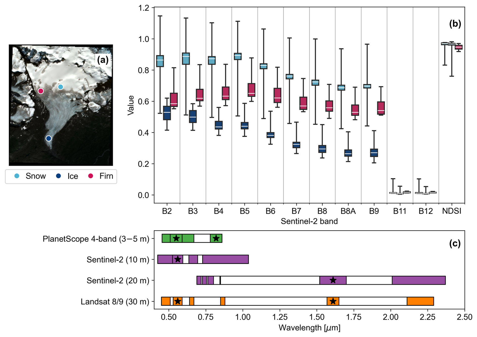
Figure 1 (a) Copernicus Sentinel-2 surface reflectance image at Wolverine Glacier, AK, captured on 17 August 2020 and snow, ice and firn sample point coordinates. (b) Boxplots of band reflectance values and the Normalized Difference Snow Index (NDSI) at each of the sample points shown in panel (a) for 45 selected Sentinel-2 SR images spanning late June to early October 2019–2023. Reflectance values were extracted from each fixed point but only in images where these points could be confidently identified as covering their respective surface material. For example, ice reflectance values were sampled from images where the ice coordinate in panel (a) was clearly covering ice. Boxes indicate the 25th and 75th percentiles, whiskers indicate the minimum and maximum values, and white lines indicate the median. (c) Satellite image band ranges with stars indicating the bands used to calculate the NDSI. For Sentinel-2 and Landsat 8 and 9, the NDSI is calculated using the green and SWIR bands. Because PlanetScope does not have a SWIR band, the NDSI is instead calculated using the green and NIR bands.

The SCA has previously been mapped using a number of thresholding and machine learning techniques. The Normalized Difference Snow Index (NDSI) leverages the distinct contrast in visible and shortwave infrared (SWIR) reflectance between snow, ice, and firn compared to other materials (Hall and Riggs, 2007). A simple thresholding approach – NDSI > ∼ 0.4 is snow – has been used to map the SCA on non-glacier surfaces using various satellite images, such as MODIS (Salomonson and Appel, 2004), Landsat (Riggs et al., 1994), and Sentinel-2 (Gascoin et al., 2019). However, the NDSI thresholding method cannot be used over glaciers due to the overlapping NDSI ranges for snow, ice, and firn (Fig. 1b). Otsu thresholding (Otsu, 1979), which is an automated threshold selection approach for gray-level images, has also been used to map glacier snow lines but has only been tested with Landsat 8 imagery (Prieur et al., 2022; Rastner et al., 2019). Several sensor-specific machine learning techniques have also been tested: neural networks with PlanetScope imagery (Cannistra et al., 2021; John et al., 2022), random forest with Sentinel-2 imagery (Zeller et al., 2025), and support vector machine with C-band synthetic aperture radar imagery (Callegari et al., 2016; Huang et al., 2013). Despite these advancements, there remains a need for cross-sensor SCA-mapping techniques, particularly on glacier surfaces.

Our goals in this work are two-fold: (1) develop an automated snow detection workflow calibrated to glacier surfaces by evaluating several machine learning algorithms and (2) compare the results from individual image products and snow cover metrics to assess the potential for capturing spatiotemporal trends in glacier snow cover. Below, we describe the approach to address these goals, including the study sites used to construct the training, testing, and validation datasets (Sect. 2); the model training, testing, and validation dataset construction (Sect. 3.1); image pre-processing steps (Sect. 3.2); the classification model development and application (Sect. 3.3); snow line detection from the classified images (Sect. 3.4); and performance assessment of the image classifiers and snow line detection method (Sect. 3.5). We then present results for the performance assessment (Sect. 4.1) and evaluate spatiotemporal patterns of the snow cover time series at the U.S. Geological Survey (USGS) Benchmark Glacier Project glaciers (hereafter referred to as USGS Benchmark glaciers; Sect. 4.2). In the Discussion, we outline remaining challenges for glacier snow detection (Sect. 5.1), assess which image product and snow cover metric derived from the workflow produces the most robust glacier snow cover time series (Sect. 5.2–5.3), and, finally, outline the broader implications of the workflow (Sect. 5.4).

2 Study sites

Five of the mountain glaciers in this study are part of the U.S. Geological Survey (USGS) Benchmark Glacier Project, which began in 1957 (Meier, 1958) as part of a long-term initiative to document and understand connections between glaciers and climate (O'Neel et al., 2019). The project includes seasonal field and remote sensing data collection of glacier mass balance at five glacier sites located across the western contiguous United States and Alaska. These glaciers have diverse characteristics, such as aspect, latitude, continentality, and elevation (Fig. 2), all of which influence local climate regime and glacier mass balance. Gulkana Glacier is located in the Alaska Range, with an elevation range of 1235–2445 m; Wolverine Glacier is located in the Kenai Mountains of Alaska (472–1673 m); Lemon Creek Glacier is located at the southernmost tip of the Juneau Icefield in Alaska (663–1500 m); Sperry Glacier is located in Glacier National Park in Montana (2274–2791 m); and South Cascade Glacier is located in the northern Cascade Range in Washington state (1635–2204 m). Multitemporal boundaries and digital elevation models (DEMs), constructed using Maxar stereo satellite imagery and the Ames Stereo Pipeline (Shean et al., 2016), are available at each site from the USGS (U.S. Geological Survey Benchmark Glacier Program et al., 2022). Despite the diverse climatic and terrain conditions of the USGS Benchmark glaciers, these sites do not represent the full suite of complexity in glacier surface types, due to limited debris cover and elevation range. To ensure that the classification workflow can be applied to glacier characteristics that are more challenging for image classification than the Benchmark glaciers, we also included Emmons Glacier in Washington state in the performance assessment (Fig. 2f). Emmons spans a larger elevation range and has more frequent topographic shading, extensive debris cover, and patchy snow and other surface types particularly late in the melt season.

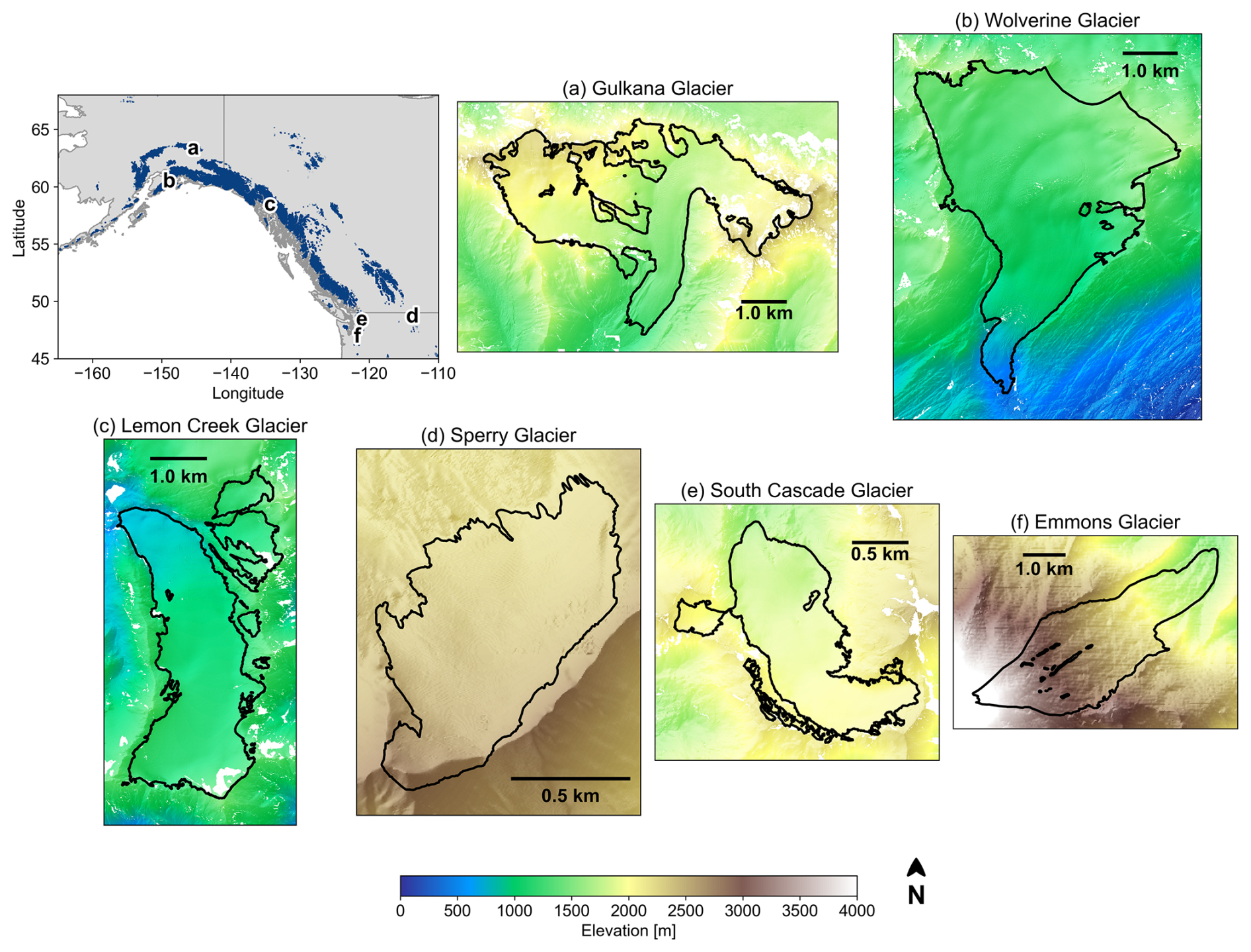
Figure 2 Maps of the study sites in order of decreasing latitude. Upper left: locator map of study sites with all identified glaciers in the region shaded in blue (Randolph Glacier Inventory regions 1 and 2; RGI Consortium, 2017) and country outlines shown in gray. (a)–(f) Shaded relief maps with glacier boundaries outlined in black for the USGS Benchmark glaciers and Emmons Glacier in Washington state. For the Benchmark glaciers, digital elevation models (DEMs) and glacier boundaries are from the USGS data release version 8 (U.S. Geological Survey Benchmark Glacier Program et al., 2022) for the most recent date. For Emmons Glacier, the DEM is from the NASADEM (NASA JPL, 2020), and glacier boundaries are from the Randolph Glacier inventory version 6 (RGI Consortium, 2017).

3 Methods

We developed an automated snow detection workflow by testing nine supervised machine learning (ML) models (listed in Sect. 3.3) applied to Landsat 8 and 9, PlanetScope, and Sentinel-2 satellite image products. The model training and testing data used to select the optimal ML classifier for each image product were constructed for four glaciers in North America that sample midlatitudes and high latitudes and maritime and continental climate regimes (Fig. 2a–b, d–e). To assess the performance of each ML image classifier, we compared automated SCA maps and snow lines to a separate validation dataset comprised of manually generated snow cover observations at two additional glacier sites (Fig. 2c, f). The image classifiers were then used to construct SCA maps at each site for 2013–2023. From the SCA maps, we extracted time series of the transient accumulation area ratio (AAR), the snow line, and the median snow line altitude. The transient AAR offers a normalized representation of glacier SCA with respect to its total area over time. At the end of the melt season, the AAR provides insights into the fraction of the glacier area with positive surface mass balance. The study sites selected for workflow development and ML model testing and validation, as well as detailed descriptions of the workflow steps, are described in the subsections below.

3.1 Training, testing, and validation dataset construction

To construct the model training, testing, and validation datasets, we manually classified more than 8000 points for each image product (∼ 32 000 points total) as snow, shadowed snow, ice–firn, rock, or water in several images at the USGS Benchmark glaciers and Emmons Glacier. We also explored the inclusion of a dedicated firn class that was distinct from the ice–firn class. To develop this dedicated firn class, we used manually classified points at Wolverine Glacier, where firn is visible on the surface late in the melt season most years (Fig. 1a). However, we found that including the dedicated firn class increased misclassifications and that the performance of the supervised ML snow detection workflow was superior using the ice–firn class. Classified points from Gulkana, Wolverine, South Cascade, and Sperry glaciers were combined to construct the training–testing dataset and points from Lemon Creek and Emmons glaciers were set aside for validation. We consider Lemon Creek Glacier a relatively ideal site for classification given its simple geometry, limited topographic shading, and typically continuous snow cover on the surface without exposed debris or surface water, for example (Fig. 2c). On the other hand, Emmons Glacier is a more challenging site for classification of snow because of its abundant debris cover, topographic shading, and patchy snow near the end of the melt season (Fig. 2f).

Points in each image were chosen using stratified random sampling (Cochran, 1977) such that the number of points chosen for each class was roughly proportionate to the areal coverage of the class (Fig. 3). Images were selected to span different months of the melt season in an effort to capture a wider distribution of reflectance values for each class (i.e., surface type). This sampling method led to the most snow-covered points due to the larger relative area of snow early in the melt season. We tested several configurations of the training dataset (e.g., stratified proportional sampling) and found little to no impact on the classification accuracies and results. We avoided points close to the snow–firn or snow–ice boundary where the class distinction was unclear to minimize bias associated with user interpretation. Only a small fraction of the points classified as ice were most likely firn based on previous field observations, given the difficulty in interpretation in most cases. At each classified point, all visible, infrared, and thermal band values were sampled from the respective pre-processed satellite image (image pre-processing described in Sect. 3.2). Next, we calculated the NDSI for each point as the normalized difference between the green and shortwave infrared (SWIR) bands for Landsat and Sentinel-2. Because PlanetScope does not include a SWIR band, the NDSI for each PlanetScope pixel was instead calculated using the green and near-infrared (NIR) bands. The normalized difference of the green and NIR bands theoretically captures the distinct signatures of snow, ice, and firn compared to other materials, similar to that of the green and SWIR bands in other image products (Fig. 1c).

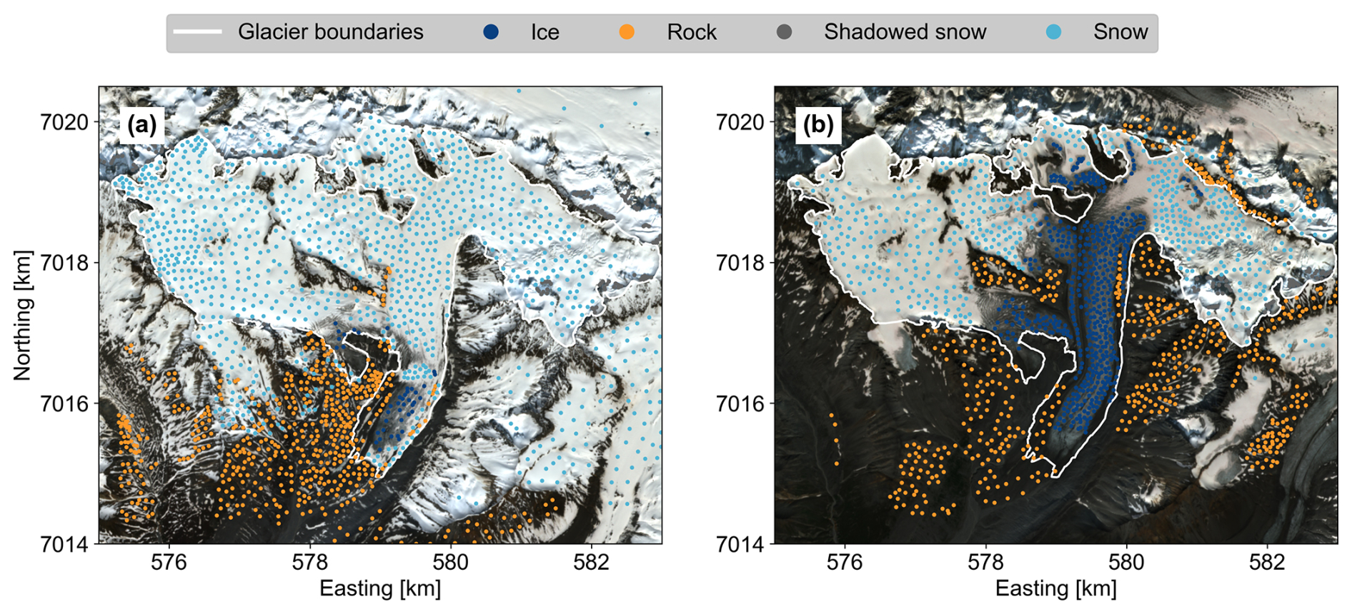
Figure 3 Example of manually classified points used to construct the training–testing dataset at Gulkana Glacier, Alaska. Points are shown for two Sentinel-2 surface reflectance images captured: (a) 15 June 2021 and (b) 6 August 2021. Coordinates are with respect to UTM zone 6N. Images ©2021 Planet Labs PBC.

3.2 Image pre-processing

To optimize temporal coverage of glacier SCA time series, we developed the snow detection workflow using Landsat 8 and 9, PlanetScope, and Sentinel-2 imagery. The characteristics of each satellite image product are listed in Table 1. We preferentially selected surface reflectance (SR) products rather than top-of-atmosphere (TOA) reflectance products, because the atmospheric corrections on SR products generally allow for better change detection on the Earth's surface (Masek et al., 2006). However, because Sentinel-2 SR imagery has only been available since 2018, we also included all Sentinel-2 TOA products available since 2015 to increase temporal coverage. Additionally, even though the PlanetScope images used in this analysis were harmonized with Sentinel-2 as the target sensor (Planet Labs PBC, 2023), we still found a wide distribution of dynamic ranges between images. For example, the maximum SR values for two images at the same site captured under similar conditions are 0.8 and 1.5. To better unify the imagery, we developed an additional pre-processing step for PlanetScope imagery described in the Supplement (Sect. S1). Briefly, the median SR values in the highest elevation portions of each glacier were assumed to consist primarily of snow such that the SR dynamic range was adjusted to vary from zero (for the darkest pixels) to 0.94 for the blue band, 0.95 for the green band, 0.9 for the red band, and 0.78 for the near-infrared band, based on SR of fresh snow from Painter et al. (2009). Although this adjustment relies on the potentially biased assumption that the upper elevations contain fresh snow, we found that this step improved the overall accuracy of PlanetScope snow detection.

To capture the evolution of glacier snow cover throughout the ablation season, we accessed all images from each product from 1 May to 1 November (Fig. 5, step 1), which encompasses all 21st century minimum mass balance dates recorded for the USGS Benchmark glaciers (U.S. Geological Survey Benchmark Glacier Program et al., 2022). We accessed Landsat and Sentinel-2 images through the Google Earth Engine data repository and Sentinel-2-harmonized PlanetScope four-band surface reflectance scenes through the Planet Labs PBC Python API. The time series spans 2013, when Landsat 8 was launched, to 2023 (Table 1). Images were clipped to the closest glacier boundary in time (RGI Consortium, 2017; U.S. Geological Survey Benchmark Glacier Program et al., 2022) and masked for clouds, heavy haze, and cloud shadows using the “geedim” Python package for Landsat and Sentinel-2 images and the Usable Data Mask associated with each PlanetScope image (Planet Labs PBC, 2023). A data table showing the timestamps of each glacier boundary and DEM for each snow detection year is provided in the Supplement (Sect. S2, Table S1). While the cloud masks are subject to occasional errors, particularly for PlanetScope, we found that large clouded areas were typically identified by the cloud masks, and using them to mask images improved the time series of classified images overall. To maximize spatial coverage, all images captured within the same hour by the same satellite, typically consisting of images with distinct but overlapping footprints, were used to construct an image mosaic (Fig. 5, step 1). Through the process of mosaicking, the images were spatially aligned, and the median of the overlapping pixels was used to eliminate abrupt mosaic edges. All image mosaics with less than 70 % coverage of the glacier area were then removed from the analysis. After testing a number of thresholds, we found that the 70 % threshold sufficiently filtered very cloudy and hazy images while preserving the highest number of clear, usable images for our study sites. Nonetheless, we suggest testing different thresholds when applying the workflow to other sites.

Table 1 Data products used in the automated snow detection workflow.

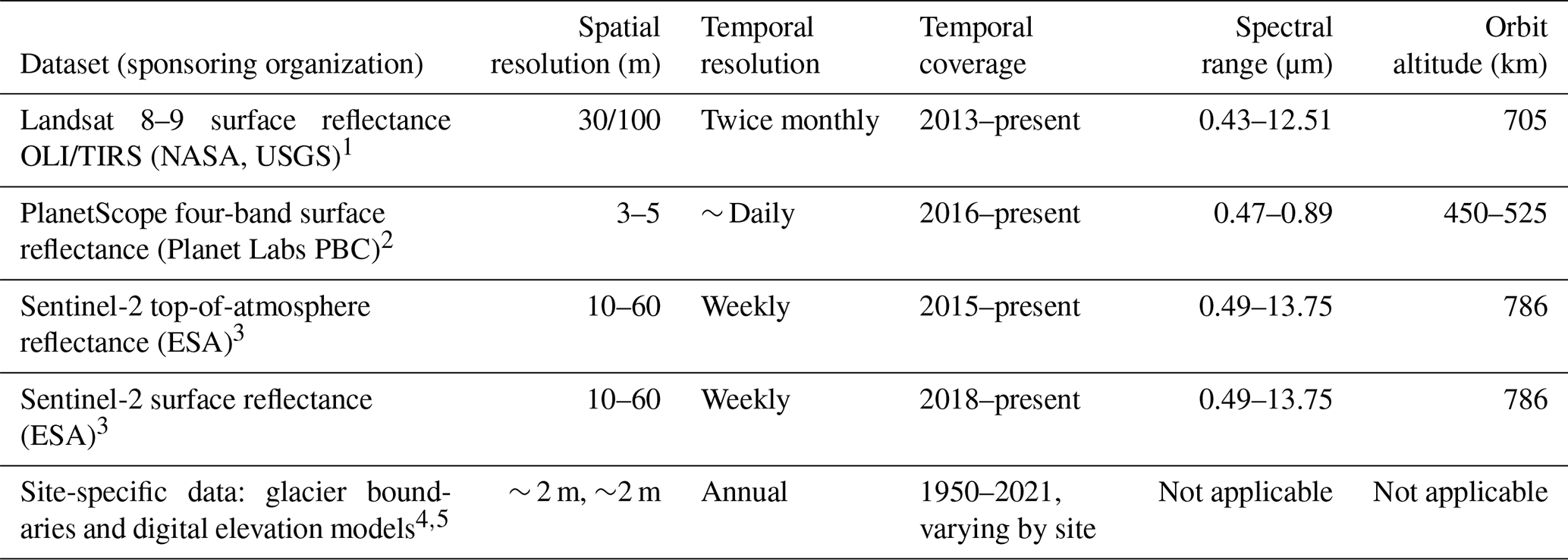
¹ U.S. Geological Survey (2015). ² Planet Labs PBC (2023). ³ European Space Agency (2015). ⁴ U.S. Geological Survey Benchmark Glacier Program et al. (2022). ⁵ RGI Consortium (2017).

3.3 Classification models development and application

In recent decades, ML models have been increasingly used for land cover classification (Thanh Noi and Kappas, 2018). ML models exhibit exceptional proficiency in handling multidimensional data (such as many image bands) and complex class characteristics (Maxwell et al., 2018), potentially making them an ideal tool for distinguishing snow from other surface types in glacierized environments. Supervised ML models, which require user-constructed training data, tend to outperform unsupervised models in land cover classification applications (Bahadur K. C., 2009; Boori et al., 2018).

For each image product, we trained and tested nine supervised ML models: linear (logistic regression, nearest neighbors), quadratic (quadratic discriminant analysis), non-parametric (decision trees), kernel-based (support vector machine), ensemble (AdaBoost, random forest), naïve Bayes, and neural network models (Fig. 4). Due to the unique band characteristics of each image product (Fig. 1c), a separate ML model was required for each product. While the support vector machine, random forest, nearest neighbors, and neural network models are generally reported to be foremost models for land cover classification (Thanh Noi and Kappas, 2018; Wang et al., 2021), we tested several others because our classes are unique from typical land cover classification applications. ML models were accessed through the Python-based scikit-learn toolbox (Pedregosa et al., 2011). Hyperparameters for each ML model are shown in the Supplement (Sect. S3; Table S2). For more information on the mathematical basis and implementation of each machine learning model, refer to the scikit-learn documentation (https://scikit-learn.org/stable/user_guide.html, last access: 10 April 2025).

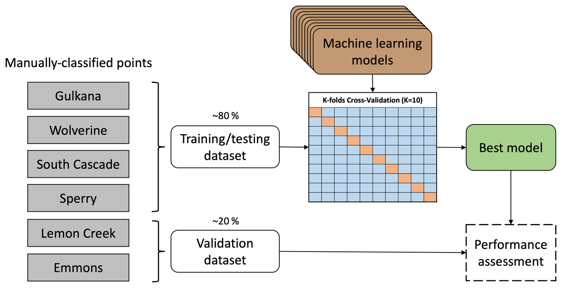
Figure 4 Schematic of the machine learning model training, testing, and validation process conducted for each satellite image product separately.

The optimal model for each image product was determined using K-fold cross-validation (Hastie et al., 2009) with K=10, wherein the training–testing dataset was split into 10 equally sized subsets, or “folds”. The model was trained using nine folds and then tested on the remaining fold, iterating this process until all folds were set aside and used to calculate the overall accuracy (Fig. 4). The model with the highest mean overall accuracy was determined to be the optimal model for each image product and retrained using the full training dataset. To investigate the robustness of our model selections, we also calculated learning curves for each ML model, which provide insight into the dependence of a model's performance on the training dataset size (Viering and Loog, 2023), detailed in the Supplement (Sect. S4; Fig. S2).

The optimal classification models were then applied to their respective pre-processed image collections at the USGS Benchmark glaciers, resulting in classified image collections at each site (Fig. 5, step 2). The SCA for each image was calculated as the total number of snow-covered pixels (both “snow” and “shadowed snow” classes) within the glacier boundary, discarding masked pixels, and multiplied by the appropriate pixel resolution. The AAR was calculated using the ratio of the SCA to the total glacier area.

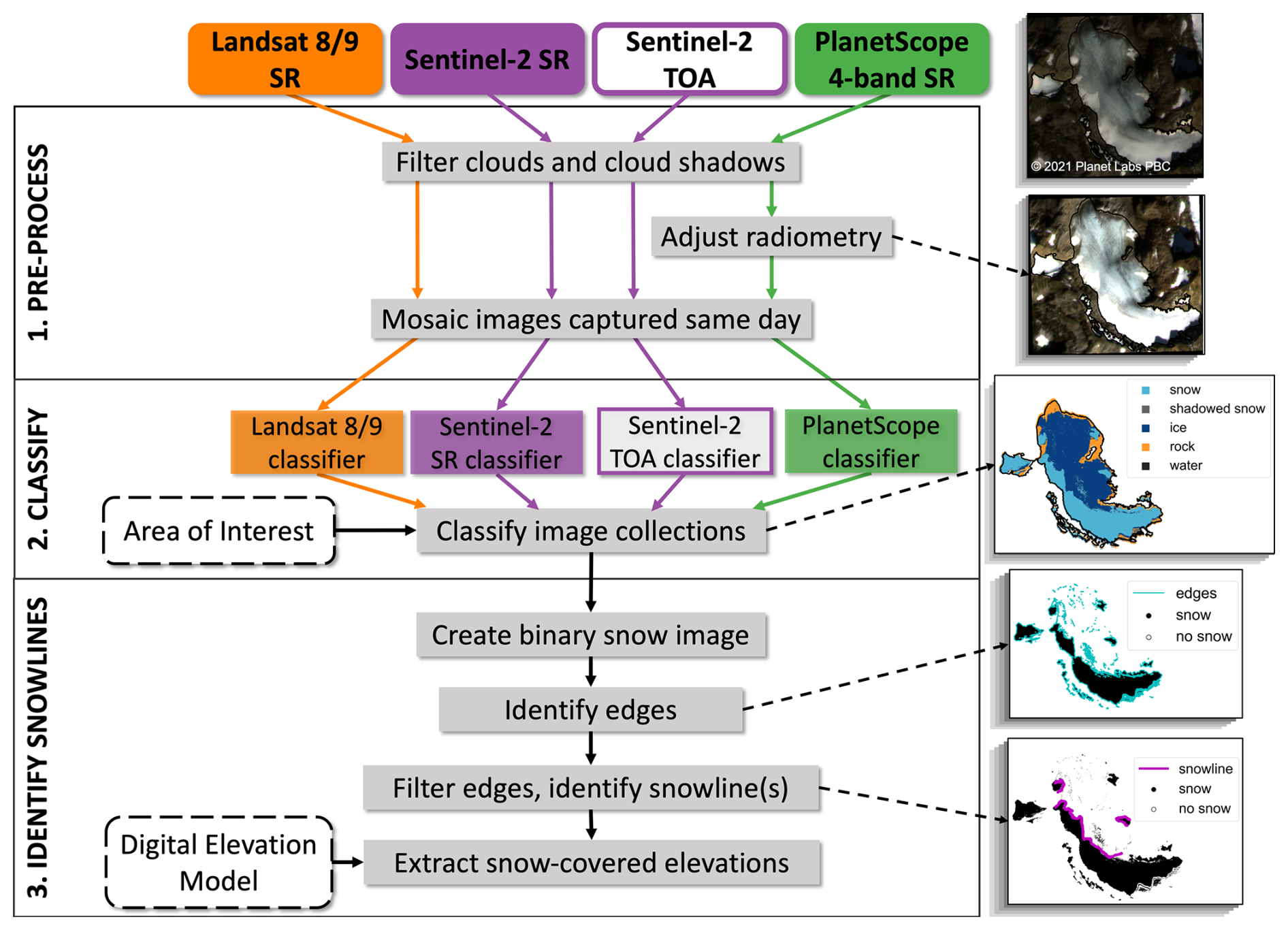
Figure 5 Schematic of the image processing workflow. Images on the right show example results for a PlanetScope surface reflectance image captured at South Cascade Glacier, Washington state, on 24 September 2021, where dashed black arrows point to the corresponding processing step. Image ©2021 Planet Labs PBC.

3.4 Snow line detection

Seasonal snow lines were automatically identified by adjusting and analyzing the classified images (Fig. 5, step 3). Our general approach for snow line detection was to identify the longest boundaries between snow and other classes in each classified image. To prevent the snow line from being detected within the SCA, such as in areas of exposed bedrock or crevasses or in small patches of snow, classified images were adjusted using the distribution of snow-covered pixels and the boundaries between snow and no snow (“edges”). Assuming that elevation is a primary driver of snow cover distribution and glacier mass balance (e.g., Anderson et al., 2014; Cuffey and Paterson, 2010; McGrath et al., 2018), we first filled holes in the SCA maps using glacier hypsometry. For each glacier, we generated a reference elevation histogram for the entire glacier area using the closest high-resolution (∼ 2 m; Table 1) DEM in time. Next, we generated histograms of snow-covered elevations for each SCA map with 10 m increment bins spanning the glacier elevation range. We constructed a normalized histogram representing the percentage of each elevation bin covered in snow by dividing the snow-covered elevation histogram by the glacier elevation histogram. After testing a number of thresholds, all elevation bins with at least 75 % snow coverage were set to 100 %, and the classified image pixels, including cloud-masked pixels in the glacier area, were adjusted accordingly. Next, we created binary snow masks (“snow” or “non-snow”) and identified the edges between snow and no snow using an edge detection function from the scikit-image package (Walt et al., 2014) built on the marching squares algorithm (Lorensen and Cline, 1987). The no-data mask associated with the binary snow image includes all pixels outside the glacier area and cloud-masked pixels not filled in the previous histogram-based filling step. The no-data mask for each image was then buffered by 30 m (the coarsest image spatial resolution) to remove edges identified at data boundaries. To minimize detection of isolated low-elevation snow patches, edges with gaps spanning more than 100 m were split into separate edge segments, and edge segments with total lengths less than 100 m were removed, resulting in the final snow line(s). Elevations were then extracted from the DEM for each snow line vertex coordinate, which were used to track the distribution of snow-covered altitudes and the median snow line altitude over time. The final snow lines consist of coordinates at the spatial resolution of the input image.

In summary, the workflow produces classified image collections at the spatial resolution of each input image and data tables containing statistics for each classified image and snow line. Statistics include the SCA, transient AAR, snow line coordinates, surface elevations at each snow line coordinate, and the median snow line altitude.

3.5 Performance assessment

To assess the performance of each machine learning algorithm, we evaluated the snow cover classification (Sect. 3.5.1) and snow line detection (Sect. 3.5.2) results against manually classified points and manually delineated snow lines. These assessments serve to validate both the raster (classified images) and vector (snow line) products from the workflow.

3.5.1 Snow cover classification

To evaluate the performance of the ML models, we applied the classification algorithm to two glaciers that were excluded from the model training process: Lemon Creek and Emmons glaciers (Fig. 4). The classified maps for Lemon Creek and Emmons glaciers were compared to the validation set of approximately 5000 manually classified points. To focus on the accurate mapping of SCA on the glaciers, the validation points were classified as either “snow” (snow and shadowed snow classes) or “non-snow” (including ice, firn, water, and rock/debris).

Each image classifier's performance was assessed using the overall accuracy, Cohen's κ score, recall, precision, and F score (or F₁ score) metrics. To calculate these metrics, we sampled the SCA maps generated by the ML models at each manually classified point, assuming the manually classified points to be ground truth. The overall accuracy is the portion of correctly classified pixels (Campbell and Wynne, 2011):

$$\begin{array}{}\text{(1)}& \mathrm{overall}\mathrm{accuracy}={\displaystyle \frac{\mathrm{true}\mathrm{positives}+\mathrm{true}\mathrm{negatives}}{\mathrm{number}\mathrm{of}\mathrm{samples}}}.\end{array}$$

Cohen's κ score accounts for potential random agreement between the classified image and the validation points:

$$\begin{array}{}\text{(2)}& K={\displaystyle \frac{\mathrm{observed}-\mathrm{expected}}{\mathrm{1}-\mathrm{expected}}},\end{array}$$

where “observed” is the overall accuracy, and “expected” is the correct classification due to chance (Cohen, 1960). The κ score ranges from −1 to +1, with positive values indicating that the trained model performs better than a random model. For example, a random classification model with two classes (e.g., “snow” and “non-snow”) would have an “expected” overall accuracy of 0.5 (50 %). If the accuracy of the trained model, or “observed” accuracy, were 0.85 (85 %), this would result in a κ score of 0.7.

Recall generally indicates the classifier's ability to identify all positive (“snow”) samples:

$$\begin{array}{}\text{(3)}& \mathrm{recall}={\displaystyle \frac{\mathrm{true}\mathrm{positives}-\mathrm{true}\mathrm{negatives}}{\mathrm{true}\mathrm{positives}+\mathrm{true}\mathrm{negatives}}}.\end{array}$$

Precision represents the classifier's ability to not label a negative sample as positive (i.e., not to label “non-snow” as “snow”):

$$\begin{array}{}\text{(4)}& \mathrm{precision}={\displaystyle \frac{\mathrm{true}\mathrm{positives}}{\mathrm{true}\mathrm{positives}+\mathrm{false}\mathrm{positives}}}.\end{array}$$

For example, consider a binary classification problem where 30 pixels are snow and 70 pixels are non-snow. If the model classified 20 pixels as snow, out of which 15 are actually snow (true positives) and 5 are non-snow (false positives), and the remaining 10 pixels snow are incorrectly classified as non-snow (false negatives), this would result in a recall of 0.6 (60 %) and a precision of 0.75 (75 %). These metrics indicate that the model identified 60 % of all snow pixels in the dataset, and when the model classified snow pixels, it was correct 75 % of the time.

Finally, F score reflects both false positives and false negatives of the classifier using the harmonic mean of precision and recall:

$$\begin{array}{}\text{(5)}& F\mathrm{score}=\mathrm{2}\cdot {\displaystyle \frac{\mathrm{precision}\cdot \mathrm{recall}}{\mathrm{precision}+\mathrm{recall}}}.\end{array}$$

The F score ranges from 0 to 1, with higher values indicating both high precision and high recall, giving equal weight to precision and recall. Given a recall of 0.6 and a precision of 0.75 as above, the F score would be 0.67.

3.5.2 Snow line detection

To assess the performance of the automated snow line detection method, we used cloud-free PlanetScope imagery to manually delineate snow lines at each USGS Benchmark Glacier for approximately five dates per year spanning the summer melt season for 2016–2022. The manually delineated snow lines were then interpolated to ensure equal spacing with a ground resolution of 30 m, the coarsest satellite image resolution. Automatic snow lines for Landsat and Sentinel-2 imagery were only compared when the image capture date was within 1 week of the respective PlanetScope image. For each pair of manually and automatically delineated snow lines, we calculated the distance between each coordinate of the manually delineated snow line and the nearest corresponding point on the automatically detected snow line (i.e., ground distance) and the difference in median snow line altitude.

Field-based annual ELA estimates that are independent of imagery and the supervised ML approach are available for the USGS Benchmark glaciers. However, direct comparison with our snow line altitudes is hindered by methodological differences. Specifically, the USGS calculates ELAs as the elevation where surface mass balance is equal to zero according to a piecewise linear regression fit to in situ point measurements of mass balance. In situ measurements are collected on field campaigns that target favorable weather windows near the annual mass minimum, typically in August or September of each year (O'Neel et al., 2019). However, the USGS method lacks control for ELA estimates that extend beyond the glacier's elevation range. For example, this can occur in a strong negative balance year, when the fitted gradient approach extrapolates the equilibrium balance altitude above the glacier, resulting in ELA estimates that surpass the actual elevation limits of the glacier even for years where a small accumulation zone on the glacier surface persists. Consequently, such estimates fall outside the bounds of our snow line delineation method, presenting a methodological artifact that may or may not be a robust representation of the real-world conditions. Therefore, we focused our assessment on comparing the automatically and manually detected snow lines. Nonetheless, our image-based snow cover estimates may be used to help constrain ground-based ELA estimates by the USGS and other communities.

4 Results

4.1 Performance assessment

4.1.1 Snow cover classification

Here, we outline the performance assessment of the optimal ML models for snow classification. Assessments of all other tested machine learning (ML) models (n=9) are presented in the Supplement (Sect. S4, Table S3). Results for the snow cover classification and snow line detection performance with respect to manual, image-based observations using the optimal ML models are shown in Table 2.

Each ML model exceeded 83 % values across all performance metrics. The optimal models are the nearest neighbors model for the Landsat and PlanetScope SR image products and the support vector machine model for the Sentinel-2 SR and TOA image products. All classification models have an estimated overall accuracy of at least 92 %, a Cohen's κ score greater than 83 %, and an F score of at least 93 %. The Sentinel-2 SR support vector machine classifier performs best according to the performance metrics, with an overall accuracy of 98 %, a κ score of 96 %, and an F score of 98 %. The Landsat classifier is the least accurate of all optimal image product classifiers, yet it still yields an overall accuracy of 92 %.

The learning curve analysis revealed that varying the training dataset between 500 and 6500 sample points did not meaningfully change which model was the most accurate and led to minimal fluctuations (±5 %) in cross-validated accuracy scores for the optimal models. This consistent performance instills confidence that the optimal models are not prone to overfitting and are robust for all training dataset sizes greater than ∼ 1500 points. The learning curves for all models are shown in the Supplement (Sect. S4, Fig. S2).

4.1.2 Snow line detection

Automatically detected snow lines differ from manually delineated snow lines by a median of 156 m (interquartile range (IQR) of 60 to 332 m) in ground distance and by a median of −31 m (IQR of −73 to 0 m) in median elevation. Thus, the automatically detected snow lines tend to be slightly lower in elevation than the manually delineated snow lines (Fig. 6). Sentinel-2 SR and TOA automatically derived snow lines are the closest to the manually delineated snow lines, with median differences in elevation of −16 m (IQR of −46 to 0 m) and −20 m (IQR of −66 to 4 m), respectively. In terms of image pixels, Sentinel-2 SR automatically derived snow lines are within a median of 3 pixels of manually delineated snow lines. While Landsat yielded the highest disagreement in terms of ground distance, it yielded a median distance of 14 (IQR of 6 to 20) pixels from manually delineated snow lines, slightly better than PlanetScope, which had a median pixel distance of 20 (IQR of 5 to 66) pixels. Potential explanations for the varying agreement between manually and automatically detected snow lines for each image product are discussed in Sect. 5.1.

Table 2 Performance of the snow detection workflow for each satellite image product. SR indicates surface reflectance, and TOA indicates top-of-atmosphere reflectance. Snow line statistics indicate the median ± the interquartile range of differences for all dates and sites tested, where negative differences indicate that the automated snow line estimates are lower in elevation than the manually delineated snow lines. Median ground distances for automatically detected snow lines are also reported with respect to distance in pixels (px) for each image product.

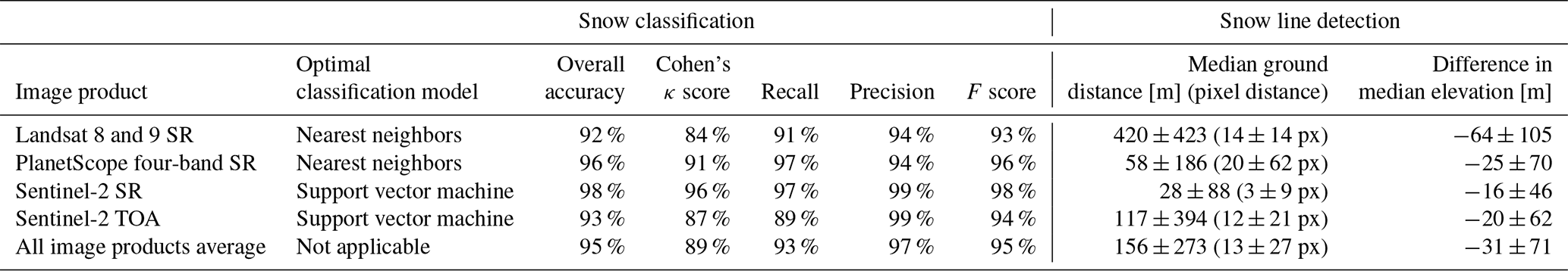
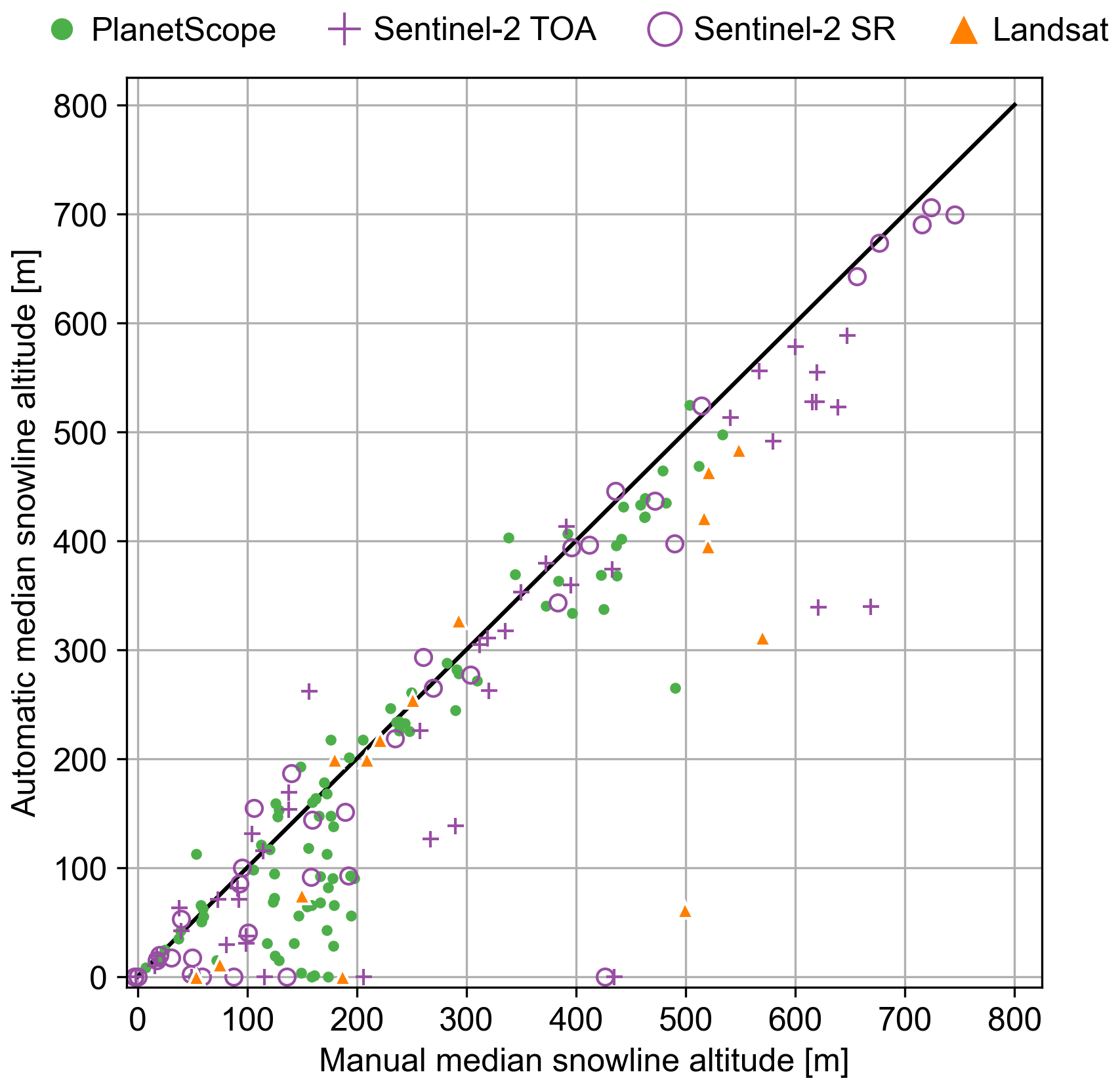
Figure 6 Manually vs. automatically detected median snow line altitudes with marker types and colors distinguishing each satellite image product. For a direct comparison across sites, snow line altitudes are reported relative to each glacier's minimum elevation.

4.2 Snow cover time series

Figure 7 shows the full time series of SCA for the USGS Benchmark glaciers using Landsat, PlanetScope, and Sentinel-2 imagery, and Fig. 8 shows the weekly median trend and interquartile range in the normalized SCA (i.e., the transient AAR) and median snow line elevation from the Sentinel-2- and Landsat-derived observations for the full 2013–2023 time series. We focus on Sentinel-2- and Landsat-derived snow cover time series because the PlanetScope-derived observations were much noisier, as evident in Fig. 7 (green circles), leading to less interpretable median trends in each snow cover metric.

The full SCA time series (Fig. 7) broadly demonstrate the density of observations in time and increasing coverage upon the launch of additional satellites from Sentinel-2 and PlanetScope starting in ∼ 2016. Notably, there is apparent interannual variability in the minimum annual SCA at some sites. For example, at Wolverine Glacier (Fig. 7b), the minimum SCA ranges from about 5 km² in 2018 and 2019 to 8–10 km² in 2021–2023. Similarly, the minimum SCA at Lemon Creek Glacier (Fig. 7c) ranges from < 1 km² in 2018 to ∼ 5 km² in 2021, highlighting the potential for assessing interannual changes in snow cover.

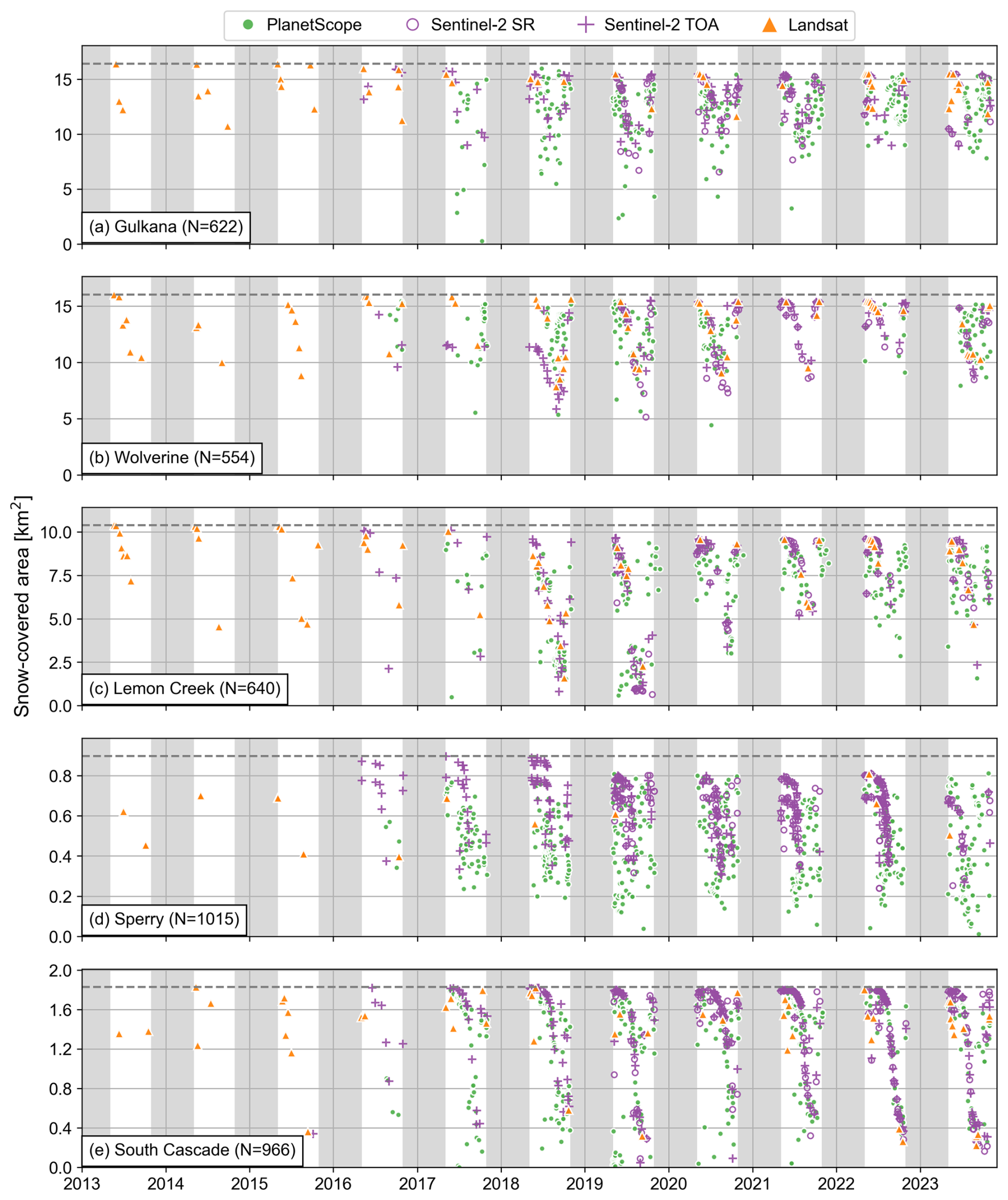
Figure 7 Time series of the snow-covered area for the USGS Benchmark glaciers with marker types and colors distinguishing each image product. Gray shaded regions indicate dates outside the observation period (1 November–30 April).

In general, the transient AAR time series suggest that the largest, most northerly sites, Gulkana and Wolverine glaciers (Fig. 8b, e), have higher annual AARs compared to other sites (Fig. 8h, k, n). Transient AARs for both Wolverine and Gulkana glaciers vary from nearly the entire glacier extent (∼ 1) in May and October to a seasonal minimum of about 0.6 ± 0.3 in August. In comparison, the average AARs are lower at Lemon Creek (∼ 0.1–0.4), Sperry (∼ 0.5), and South Cascade (0.2–0.4) glaciers. The minimum transient AAR consistently occurs in August or early September at Lemon Creek Glacier and in late September or October at Sperry and South Cascade glaciers.

On average, the onset of seasonal snow accumulation (i.e., rapid increase in the SCA) varies between sites. The decline and recovery of snow cover typically happen earliest in the year at Gulkana Glacier compared to the other sites (Fig. 8a–b). Here, the transient AAR typically declines in June, reflecting the exposure of bare ice and decline in snow cover, and reaches a minimum of about 0.5 in August. The transient AAR then increases between August and October, signaling the onset of snowfall. At Wolverine Glacier, the transient AAR both declines and recovers 1–2 weeks later than at Gulkana on average (Fig. 8c). The transient AAR time series for Lemon Creek Glacier (Fig. 8e) indicates that bare-ice exposure likely also begins in May at this site but that minimum snow cover (transient AAR of 0.5 ± 0.4) is reached in either August or September. In contrast, for both South Cascade and Sperry glaciers (Fig. 8g, i), which are both located at lower latitudes and higher average elevations than the other sites, bare ice is not exposed until June or July, with a faster decline and lower end state AAR of ∼ 0.3–0.5 in September. While these trends in SCA decline and recovery broadly correlate with site latitude, they are likely also related to other factors such as climate and elevation, as discussed further in Sect. 5.4.

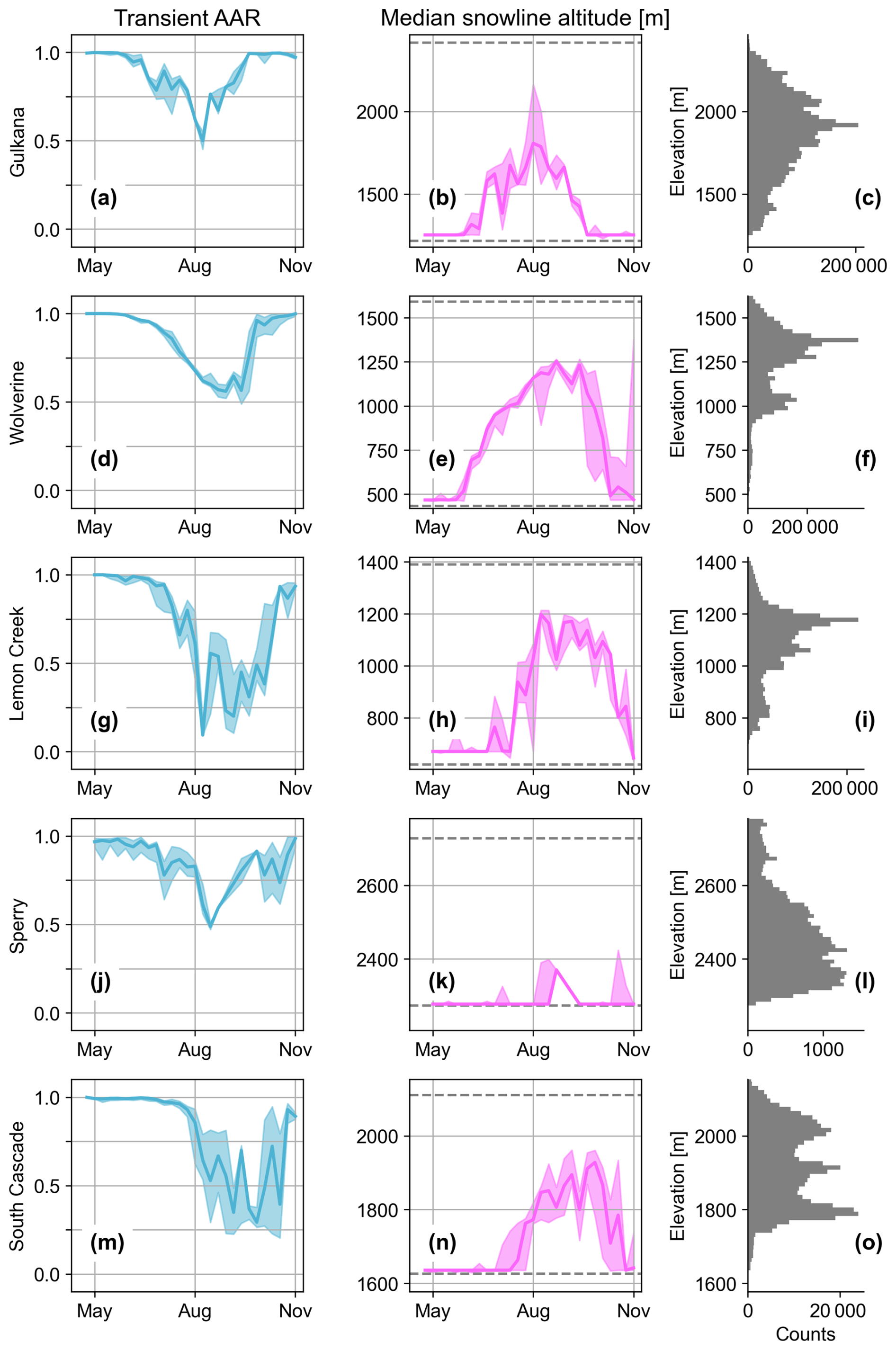
Figure 8 Weekly median trends in snow cover metrics. The left column shows transient accumulation area ratio (AAR; blue), the middle column shows median snow line altitude (pink) at each site for the full 2013–2022 time series excluding PlanetScope observations to reduce noise, and the right column shows histograms of glacier surface elevations (gray) using the most recent digital elevation model and glacier boundaries (U.S. Geological Survey Benchmark Glacier Program et al., 2022). Solid lines indicate the weekly median value, and shaded regions indicate the weekly interquartile range. Dashed gray lines in the middle column indicate the minimum and maximum glacier elevations.

5 Discussion

Leveraging multiple satellite image products and supervised machine learning algorithms, we produce detailed time series of seasonal changes in glacier snow cover. Below, we discuss challenges of the workflow associated primarily with topographic shading, cloud cover, and firn exposed on the surface. Moreover, we outline how the Sentinel-2 SR-derived observations and the transient AAR effectively overcome these limitations more consistently than other image products and metrics derived from the workflow. Finally, we analyze the SCA time series at the USGS Benchmark glaciers, highlighting variations in the timing of the snow ablation season and snow distribution patterns between sites and their implications for glacier mass balance studies.

5.1 Snow detection challenges

Complex topography, such as steep ridges along the glacier margin, can lead to less accurate SCA results due to the misclassification of shadowed snow. Sperry Glacier, for example, is particularly challenging due to its frequent topographic shading that covers a large portion of the glacier. When shade is cast by the glacier's southeastern ridge, the shaded region within the SCA is more likely to be misclassified as ice or rock. The shadowed snow class mitigates this instance of misclassification in some images (Fig. 9e–f) but not others (Fig. 9a–b). Additionally, non-continuous snow lines, characterized by large patches of bare ice within the SCA, are common at Sperry Glacier later in the melt season, which can lead to varied detection of the snow line. In these cases, the snow line may be detected within the SCA rather than at the lowest-altitude boundary separating snow and ice. Alternatively, the snow line may be divided into small segments less than 100 m in length that are filtered out before the final snow line selection. Similarly, Gulkana Glacier has multiple tributaries that flow into the main trunk. When the snow line rises above the convergence of these tributaries, the snow line may be detected in one branch but not the others, depending on the image quality and length of each snow line segment (Fig. 9c–d, g–h). In the case of multiple glacier tributaries and consistently patchy snow cover distribution, using the SCA and AAR time series to assess snow cover trends may be especially beneficial.

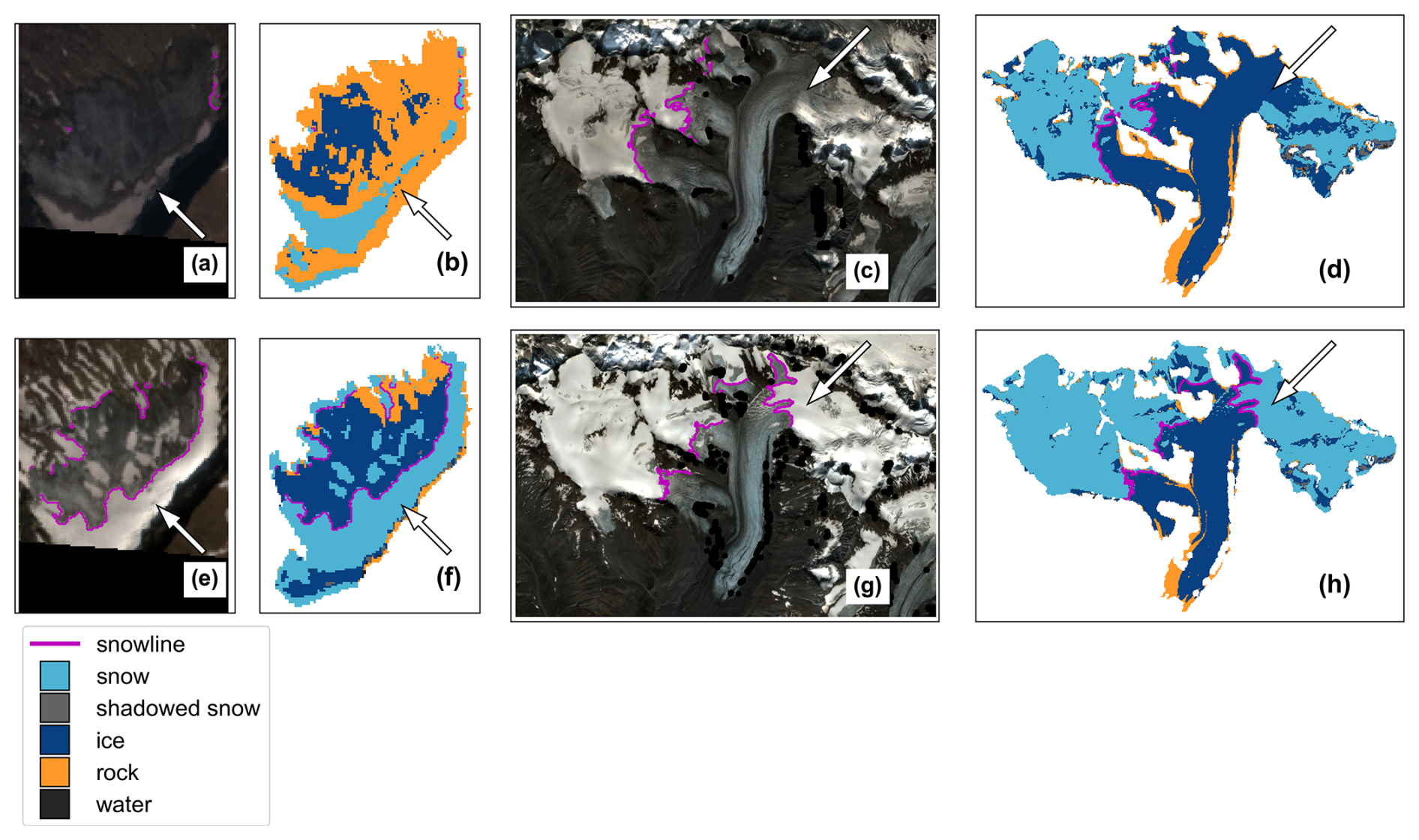
Figure 9 Sentinel-2 RGB and classified images demonstrating potential limitations of the snow detection workflow under different challenging scenarios. (a)–(b) and (e)–(f) At Sperry Glacier, topographic shading and patchy snow cover can lead to shadowed snow being misclassified as rock, with no snow line detected in some instances, indicated by the white arrows in each image. (c)–(d) and (g)–(h) At Gulkana Glacier, multiple glacier tributaries can complicate snow line detection, with varying degrees of success in different tributaries, indicated by the white arrows. Images are Copernicus Sentinel-2 data 2019: (a) top-of-atmosphere reflectance image captured 20 August 2019, (c) surface reflectance (SR) image captured 8 August 2019, (e) SR image captured 31 July 2019, and (g) SR image captured 6 July 2019.

Certain geographic regions, particularly coastal maritime sites, will have more frequent cloud cover throughout the melt season. More frequent cloud cover will result in sparser SCA time series due to either an abundance of cloudy images that are automatically filtered from the image collection or masking clouds detected in large portions of a given image. Because clouds, haze, and cloud shadows are masked in each image, the SCA and/or snow line may be fully or partially masked. The location of the site with respect to satellite ground tracks can also impact SCA accuracy. Particularly for sites that sit between satellite path boundaries with minimal overlap, the site area may exceed the coverage of images captured within the same hour, leading to consistently incomplete SCA estimates.

The distinction between the ice–firn and firn–snow boundaries poses challenges for glacier mass balance studies, including the automated snow detection workflow developed in this study. We explored the inclusion of a firn class in the classifiers using manually classified points at Wolverine Glacier, where firn is known to exist on the surface late in the melt season for most years. However, the addition of the firn class resulted in a decrease in classifier performance across all metrics due to an increase in misclassifications. We observed that the dedicated firn class was particularly sensitive to image illumination. For example, a relatively dark image would lead to most seasonal snow being incorrectly classified as firn. Given the similarity in spectral signatures among firn, snow, and ice – especially during the late melt season when seasonal snow has a lower albedo and dust and debris are more prevalent – there is substantial overlap in the spectral signatures of the training data when firn is added as a distinct class (Fig. 1b). Consequently, our classified images and snow line estimates in the absence of the firn class occasionally detect the firn–snow boundary or the ice–firn boundary, depending on factors such as ground conditions, image illumination, and the presence of clouds or haze. Rather than introduce a firn class, we suggest preferentially selecting or heavily weighting Sentinel-2 SR-derived observations when combined with those from other image products at sites where firn is known to be exposed on the surface because Sentinel-2 SR-derived classified images tend to distinguish firn from snow better than other image products. Figure 10 shows an example pair of images where the firn is problematically classified as snow in Sentinel-2 TOA imagery (Fig. 10a–b), and the firn is correctly classified as ice (not snow) in Sentinel-2 SR imagery (Fig. 10c–d) captured on the same date.

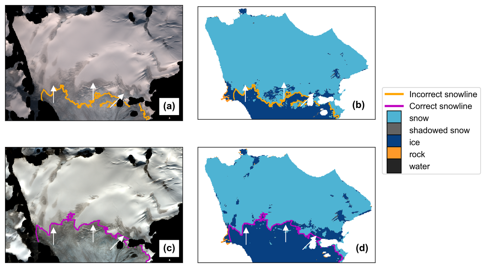
Figure 10 Example snow detection results at Wolverine Glacier demonstrating how the Copernicus Sentinel-2 surface reflectance (SR)-derived snow maps more reliably capture the snow–firn boundary than that of other image products. RGB and classified images captured 22 August 2020 from (a)–(b) Sentinel-2 top-of-atmosphere reflectance and (c)–(d) Sentinel-2 SR. White arrows point to firn exposed on the surface.

The potential impact of misclassification of firn as snow on SCA analyses will vary with the abundance of firn exposed during particularly high melt or low snow years, which depends on glacier geometry and firn extent. For instance, surface slope can substantially impact how much firn may be exposed during a relatively high melt year. Consider a 20 m rise in the snow line altitude for two glaciers of equal width: one with a constant slope of 10° and another with a constant slope of 20°. The shallower, 10° slope glacier will have a greater area of exposed bare ice and/or firn on the surface (see Sect. S5, Fig. S3, for a more detailed example and diagram). In this case, particularly for the shallower-sloped glacier and its higher sensitivity to firn misclassification, we suggest Sentinel-2 SR-derived observations be weighted more heavily when combined with observations from other image products for more consistent firn classification. Thus, the choice of image products to use when applying the workflow may depend on the specific glacier surface characteristics.

5.2 Optimizing temporal density and spatial coverage for surface mass balance assessment

High temporal resolution and coverage of SCA estimates, particularly near the end of the melt season, are critical for accurate constraints on glacier surface mass balance. While Sentinel-2 stands out as the preferred choice for generating SCA time series due to its relatively smooth time series, optimal tradeoffs between spatial and temporal resolution, and consistent snow and ice–firn discrimination, other image products contribute valuable observations.

PlanetScope has dense temporal coverage and produces classified images with overall accuracies comparable to Sentinel-2 and Landsat. However, SCA time series produced with PlanetScope imagery are noisy, meaning there is considerable scatter between observation dates relative to the Sentinel-2 and Landsat time series (Fig. 7), due to the lower image quality (i.e., differences in reflectance between images for the same earth material), cloud masking product limitations, and a narrower spectral range of PlanetScope images. The lower orbit altitude (Table 1) and lower-quality cameras compared to the governmental satellite constellations contribute to occasional saturation and less reliable cloud masks, introducing uncertainties in SCA estimates of an unknown amount. Despite efforts to normalize reflectance values between images (Sect. S1, Fig. S1), the limited spectral range of PlanetScope imagery, particularly at wavelengths beyond the near-infrared, and its frequently saturated image bands limit its ability to distinguish snow from other surface types (see Fig. 1c).

Landsat, despite its sparse twice monthly revisit time, provides valuable observations before 2016. However, the true minimum snow cover conditions may not be captured with Landsat observations alone. The longer revisit time relative to Sentinel-2 and PlanetScope, combined with frequent late summer cloud cover particularly in maritime regions, sometimes results in entire melt seasons without usable images. Challenges in time series interpretation due to the lower temporal resolution of Landsat images are pronounced for smaller glaciers like Sperry Glacier (Fig. 7d), where the likelihood of completely masked images due to cloud cover is higher.

Sentinel-2 excels in overall performance, yet observations from PlanetScope and Landsat substantially extend and add detail to the SCA time series. The unique strengths and weaknesses of each image product highlight the need for a thoughtful integration strategy to provide comprehensive insights into glacier snow cover dynamics. By combining these satellite image products, we create a robust dataset essential for comprehensive glacier mass balance studies.

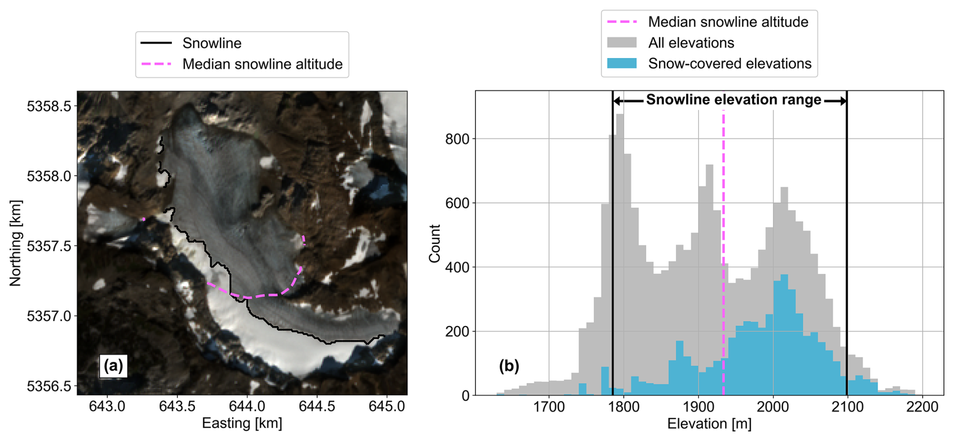
Figure 11 (a) Copernicus Sentinel-2 surface reflectance image at South Cascade Glacier captured 2 October 2023, with the automatically detected snow line and the median snow line altitude contour. (b) Histograms of all elevations in the glacier area (gray) and snow-covered elevations (blue). The pink line indicates the automatically detected median snow line altitude, and the black lines show the full elevation range (1785–2098 m) of all snow line coordinates.

5.3 Snow cover metrics comparison

While cloud cover can introduce noise into the SCA time series, the transient AAR is less impacted by cloud masking and produces the least noisy time series overall. Using the ratio of SCA to the total glacier area, the calculation of the AAR effectively counteracts the impact of heavily masked images. The automated snow line delineations can be biased by small, isolated patches or “edges” of disconnected snow that can skew the median snow line altitude. In contrast, the AAR captures snow cover at the scale of the glacier area and is therefore less sensitive to small patches of snow. In Fig. 8, the transient AAR has the lowest variability in weekly values compared to the other metrics in the early melt season, when rapid changes in snow cover are unexpected.

Additionally, the AAR does not assume that a single elevation contour on the glacier represents the zero-mass balance line, unlike the median snow line altitude or ELA. The use of a mass balance indicator with minimal assumptions is particularly important for sites where shading or other topographic effects exert a stronger influence on snow cover distribution than elevation alone. At South Cascade Glacier, for example, the steep headwalls along the southwestern boundary serve as avalanche source regions in the winter and also provide topographic shading throughout the ablation season (O'Neel et al., 2019; Fig. 11a). As a result, the automatically detected snow line in the late melt season crosses a wide range of elevations (1785–2098 m; Fig. 11b). Therefore, using the median snow line altitude as an indicator of snow cover decline and recovery rather than the transient AAR or distribution of snow-covered elevations could miss important topographic or other climate controls on snow distribution over time.

Notably, the AAR accuracy depends on a time-evolving glacier boundary (Florentine et al., 2023). Outdated boundaries can lead to misleading results in cases where the glacier area has changed in response to climate or internal dynamics. For instance, a few years of lower-than-average snowfall or higher-than-average melt can lead to glacier thinning and terminus retreat over several years (Cuffey and Paterson, 2010). If glacier boundaries are not updated over time as in this study (Table S2), the AAR will be underestimated. Thus, glacier boundaries should be updated as needed when applying the workflow.

5.4 Broader implications

The automated snow detection workflow offers substantial time savings compared to manual snow line delineation. Implementing the full workflow with pre-trained image classifiers for all satellite image products from 2013–present at one site, including PlanetScope image downloads and pre-processing, typically requires an hour or less from the user and anywhere from about 2–50 h of computation time, depending on the computing resources, size of the site, and number of images found. In comparison, manual delineation of glacier snow lines can take approximately 1–5 min per image, with additional time needed for PlanetScope image downloads. Considering that our automated method identified an average of ∼ 750 usable images per site since 2013, manually delineating all snow lines for a single site would require more than ∼ 20 h of work by the user. Adopting our automated method could save hundreds of hours for the user, particularly when applying it to multiple sites, making it an efficient approach for tracking changes in glacier snow cover on broad spatial scales.

Despite potential limitations related to shading, cloud masking, and firn misclassification affecting snow detection at individual sites, the extensive time series of image-based snow cover observations generated by this workflow holds promise for various applications. These observations can improve our understanding of current glacier AARs and ELAs, supporting glacier–climate sensitivity tests. For example, the dense time series of snow cover observations can help to constrain the timing of minimum snow cover conditions. Notably, for the Benchmark glaciers, snow-off conditions tend to occur later (June–July) at South Cascade and Sperry glaciers. Sperry and South Cascade glaciers are the lowest in latitude, with Sperry Glacier located at the highest elevations and South Cascade Glacier located in a mid-elevation, maritime climate. Snow-on conditions tend to occur earlier (September–October) at the Alaskan glaciers, which span maritime and continental climates and low elevations to mid-elevations. These findings demonstrate the valuable insights gained into the spatiotemporal variability of snow cover minimum conditions across latitudinal, climatic, and elevational ranges spanned by the Benchmark glaciers through the application of the automated snow detection workflow. Additionally, these snow cover observations can serve as inputs or observational constraints for climate modeling, offering valuable validation data for snowmelt and atmospheric modeling applications, thereby advancing our understanding of diverse Earth system interactions.

6 Conclusions

In this study, we present an automated snow detection workflow calibrated to mountain glaciers, offering several advantages over existing methods for snow classification. Our approach leverages multiple spaceborne imagery datasets, resulting in hundreds of snow cover observations spanning over a decade. Temporal resolutions range from approximately twice monthly to daily throughout the summer melt season, depending on local cloud cover conditions and generally increasing over time with the launch of additional satellites. In future work, we will apply the automated snow detection workflow more broadly to glaciers throughout North America. Additionally, the workflow may be tested in other climatic settings, such as tropical or polar glacierized environments. This would enable us to evaluate the transferability of the classification models, particularly in light of potentially distinct spectral responses of snow, ice, surface meltwater, and debris in these regions.

Using a training dataset constructed at the USGS Benchmark glaciers and supervised machine learning models, the image classification models exhibit high performance, achieving overall accuracies of at least 92 %. κ scores, which account for potential correct classification due to chance, range from 84 %–96 % for all classification models. The workflow performance and temporal coverage are impacted by a number of factors, primarily the presence and frequency of widespread shading and cloud cover at individual sites.

Among the image classification models, the Sentinel-2 surface reflectance (SR) classification model (support vector machine) produces the most accurate and smoothest snow-covered area time series (overall accuracy > 95 %), with the best agreement with manually delineated snow lines (median altitudes differ by a median of −16 m with an interquartile range of −46 to 0 m). Sentinel-2 SR-classified images also distinguish snow from ice and firn the most consistently at our study sites. Therefore, we suggest weighting Sentinel-2 SR-derived observations more heavily than those from other image products, particularly at sites where extensive firn is known to be exposed on the surface. Nonetheless, Landsat- and PlanetScope-derived observations greatly increase both the temporal coverage and frequency of observations, which are critical near the end of the melt season when snow cover changes rapidly.

Furthermore, our results reveal variation in the timing of bare-ice exposure and snowfall onset across the Arctic and midlatitude USGS Benchmark glaciers, which span 48 to 63° N. The observed spatial variations in minimum SCA for this subset of glaciers emphasize that estimating the equilibrium line altitude (ELA) based on a fixed date, such as late September, can lead to biased results depending on the glacier site. Additionally, non-elevation-dependent snow lines at South Cascade Glacier, in particular, challenge the assumption of a single ELA as an accurate approximation of the accumulation and ablation zone boundary on mountain glaciers.

The automated snow detection workflow has the potential to benefit numerous scientific disciplines and applications. By improving our understanding of glacier snow dynamics, such as snow distribution, accumulation, and ablation patterns, we not only enhance glacier monitoring but also provide a validation dataset for atmospheric, hydrological, and glacier modeling. The insights gained from our approach therefore have the potential to improve the accuracy of climate model predictions, guide water resource management, and refine our understanding of evolving snowmelt seasons.