Glacier damage evolution over ice flow timescales

The rate of mass loss from the Antarctic and Greenland ice sheets is controlled in large part by the processes of ice flow and ice fracture. Studies have shown these processes to be coupled: the development of fractured zones weakens the structural integrity of the ice, reducing ice viscosity and enabling more rapid flow. This coupling may have significant implications for the stability of ice shelves and the rate of flow from grounded ice. However, there are challenges with modeling this process, in large part due to the discrepancy in timescales of fracture and flow processes and to uncertainty about the construction of the damage evolution model. This leads to uncertainty about how fracture processes can affect ice viscosity and, therefore, projections of future ice mass loss. Here, we develop a damage evolution model that represents fracture initiation and propagation over ice flow timescales, with the goal of representing solely the effect of damage on flow behavior. We then apply this model to quantify the effect of damage on projections of glacier response to climate forcing. We use the MISMIP+ benchmark glacier configuration with the experiment Ice1r, which represents grounding line retreat due to basal melt forcing. In this model configuration, we find that damage can enhance mass loss from grounded and floating ice by ∼ 13 %–29 % in 100 years. The enhancement of mass loss due to damage is approximately of the same order as increasing the basal melt rate by 50 %. We further show the dependence of these results on uncertain model parameters. These results emphasize the importance of further studying the multiscale processes of damage initiation and growth from an experimental and observational standpoint and of incorporating this coupling into large-scale ice sheet models.

1 Introduction

Ice flow, which transports ice from ice sheet divides towards the ocean, is a significant control on the rate of ice sheet mass loss. The rate of ice flow through fast-flowing glaciers in Antarctica and Greenland has increased in the last 2 decades (Pritchard et al., 2009; Cook and Vaughan, 2010; Paolo et al., 2015; King et al., 2020; Wallis et al., 2023), enhancing the contribution of ice sheets to global sea-level rise (Rignot et al., 2011; Fox-Kemper et al., 2021). Therefore, understanding and modeling the processes that govern the rates of ice flow is of particular importance.

The observed acceleration in ice flow has, in many cases, been linked to fracturing upstream from glacier termini. Lhermitte et al. (2020) and Sun and Gudmundsson (2023) have correlated recent accelerations of ice flow at Pine Island Glacier with the development of fractures along the margins of the glacier. Surawy-Stepney et al. (2023a) similarly relate the development of fracturing in Thwaites Glacier to changes in ice flow speed. These observations have been physically explained by fractures structurally weakening the ice, thus reducing the effective bulk ice viscosity and enabling more rapid flow (Lhermitte et al., 2020; Sun and Gudmundsson, 2023). Furthermore, the accumulation of damage on ice shelves can reduce their ability to buttress grounded ice, enabling more rapid flow from grounded regions to floating ice shelves (Borstad et al., 2013, 2016; Fürst et al., 2016). Ultimately, the observed accumulation of fractures on both grounded ice and floating ice has the potential to affect ice sheet mass loss through enhanced acceleration of flow and its effect on the stability of ice shelves and ice cliffs (Bassis et al., 2024), pointing to the need for fractures to be included in ice sheet models used to predict ice flow changes.

Previous studies have taken different approaches to the modeling of fractures in ice sheets. Many studies have applied fracture mechanics principles, including zero-stress and linear elastic fracture mechanics (LEFM) theories, to understand the propagation of crevasses leading to calving (Jezek, 1984; Van Der Veen, 1998a, b; Rist et al., 2002; Benn et al., 2007b) and to predict when large-scale rifts may propagate (Lai et al., 2020). However, LEFM is limited in its ability to represent the effect of fracturing on viscous properties of a material. Firstly, defects within ice sheets range from microcracks and voids ($\sim {\mathrm{10}}^{-\mathrm{3}}$–10⁻² m) to macroscale rifts and crevasses (∼10²–10⁴ m) (Krajcinovic, 1996), and the grid size of numerical ice sheet models is too large to explicitly capture the micro- and mesoscale fractures (Van Der Veen, 1998b; Jezek, 1984; Borstad et al., 2013). Secondly, fractures evolve on far shorter timescales (∼10⁰–10⁴ s) than ice sheet models can resolve, as they are designed to model longer-timescale ($\sim {\mathrm{10}}^{-\mathrm{1}}$–10⁵ years) viscous deformation, so they typically have time steps of days to months. This discrepancy in timescales is a challenge this paper aims to tackle.

Other studies modeling ice fracture have applied the principles of continuum damage mechanics (CDM). Rather than modeling the initiation and propagation of individual cracks, continuum damage mechanics uses an internal state variable to describe the average density of defects within a representative volume of material, typically referred to as “damage” (Lemaitre, 1996; Krajcinovic, 1996; Kachanov, 1999). This enables straightforward integration of fractures into constitutive models and provides a computationally efficient way of accounting for the effects of microdefects, thus allowing a representation of the effect of material damage on mechanical deformation across spatial scales (Krajcinovic and Mastilovic, 1995).

Most of the CDM modeling studies in the glaciology literature are focused on representing calving in viscous flow models at the scale of an individual glacier or ice shelf. Pralong and Funk (2005) originally proposed using a CDM model based on the anisotropic theory for creep fracture developed by Murakami (1983), building on the works of Kachanov (1958) and Rabotnov (1968), to simulate the calving process in an alpine glacier. This creep CDM model was later extended to include temperature dependence (Duddu and Waisman, 2012), was implemented using nonlocal formulations (Duddu and Waisman, 2013a; Duddu et al., 2013; Jimenez et al., 2017; Huth et al., 2021b), and was combined with water pressure terms to represent hydrofracturing (Mobasher et al., 2016; Duddu et al., 2020). Huth et al. (2023) applied the creep CDM model to the calving of Iceberg A68, which calved in 2017, to demonstrate that it can replicate the rift propagation process during the 2 years prior to calving. As another approach to representing damage in ice sheets, Borstad et al. (2012) applied an inverse method to estimate damage on the Larsen B ice shelf prior to its collapse, as a way to constrain a calving law. A similar inverse technique was used to identify the effects that damage has on weakening ice shelves (Borstad et al., 2013, 2016; Sun and Gudmundsson, 2023). Krug et al. (2014) proposed a prognostic approach that uses a combination of CDM and LEFM models, which represents the weakening of ice due to accumulated damage and downward propagation of crevasses to eventually form rifts.

Alternatively to the creep CDM model, Bassis and Ma (2015) developed a ductile failure model to account for plastic necking and the melting/re-freezing process, which can enhance basal crevassing. Sun et al. (2017) proposed a damage model that calculated the penetration depth of surface and basal crevasses and coupled it to an ice sheet model to represent the evolution of crevasses within a shallow-shelf approximation (SSA). Kachuck et al. (2022) described damage evolution using a combination of the crevasse penetration depth model (Sun et al., 2017) and the plastic necking model (Bassis and Ma, 2015). Considering the relatively fast brittle fracture process in ice, Sun et al. (2021) and Clayton et al. (2022) developed phase field fracture models that integrate LEFM and poromechanics concepts within the CDM framework to describe the hydrofracturing of crevasses.

While the approaches described above have been primarily applied to improve the understanding of calving processes, there are comparatively few studies that incorporate such damage models for the purpose of understanding the role of damage in governing long-timescale (decadal to century-scale) changes in ice rheology and ice flow. Previously, Albrecht and Levermann (2012, 2014) presented a model framework for coupling damage evolution and flow and compared its results with present-day observations of Antarctic ice shelves. Sun et al. (2017) and Lhermitte et al. (2020) quantified the enhancement of flow due to damage evolution in forward simulations of an idealized glacier using the damage model developed in Sun et al. (2017). Despite this previous work, there remains significant uncertainty about the effects of damage on future flow, derived from the choice of damage model, the choice of parameters in the damage model, and the applied forcing.

Here, we seek to quantify the effect of damage evolution on projections of ice loss. The specific goal of this work is to constrain the effects of damage-induced weakening on flow acceleration and ice loss. As such, this work does not aim to represent the effects of damage and damage-induced weakening on the localization and propagation of rifts leading to calving. We first propose a simplified model for incorporating scalar damage evolution into flow models that takes into account the discrepancy in timescales between ice flow and ice fracture and reduces the parametric freedom within current damage models. We then apply this simplified model to a benchmark marine-terminating glacier configuration to quantify the effect of including damage into glacier flow with regard to ice mass loss.

2 Timescales of damage evolution

In the CDM framework, the density of fractures in a representative volume of material, generally called “damage”, denoted by D, can simply be treated as a scalar continuum state variable (Kachanov, 1958) and is constrained by $D\in [\mathrm{0},\mathrm{1}]$. If D=0, the material is perfectly intact, whereas, if D=1, the material has lost all of its load-bearing ability due to the accumulation of fractures and other defects (Lemaitre, 1996).

The evolution of the damage variable in ice sheets is generally described through a transport (advection–reaction) equation in the Eulerian framework:

$$\begin{array}{}\text{(1)}& {\displaystyle \frac{\partial D}{\partial t}}+\mathbf{u}\cdot \mathrm{\nabla }D=\left\{\begin{array}{ll}f,& {\mathit{\sigma }}^{†}\ge {\mathit{\sigma }}_{\mathrm{t}}\\ \mathrm{0},& {\mathit{\sigma }}^{†}<{\mathit{\sigma }}_{\mathrm{t}}\end{array}\right.,\end{array}$$

where $\mathbf{u}=(u,v,w)$ is ice velocity, f is the damage evolution function describing the rate of change of damage due to deterioration or healing, σ^† denotes a chosen invariant of the Cauchy stress tensor σ (e.g., trace or maximum principal value), and σ_t describes the stress threshold parameter above which damage begins to accumulate. While, in general, anisotropic damage must be represented as a second-order tensor, in this paper we consider isotropic damage evolution so that damage is represented by a scalar variable. The choice of the stress invariant and the stress threshold, along with the nature of the source/sink term, is not well constrained and is discussed further below. This representation uses a damage threshold based on stress, though other studies also use strain-based (Duddu and Waisman, 2013b) or strain-energy-based (Beltaos, 2002) thresholds.

In this study, we hypothesize that, for the purpose of evolving damage on long (flow) timescales, the specific nature of the damage evolution function f, which describes the small spatial-scale and timescale processes of fracture, does not need to be explicitly modeled, thus eliminating f and the parameters therein as poorly constrained parametric degrees of freedom. To test this hypothesis, below, we first conduct a scaling analysis. Next, we evaluate the timescales of fracture in a glacier flowline model and use this analysis to construct a simplified damage evolution model. Finally, we evaluate the applicability of this simplified model in different climate forcing scenarios.

2.1 Scaling analysis

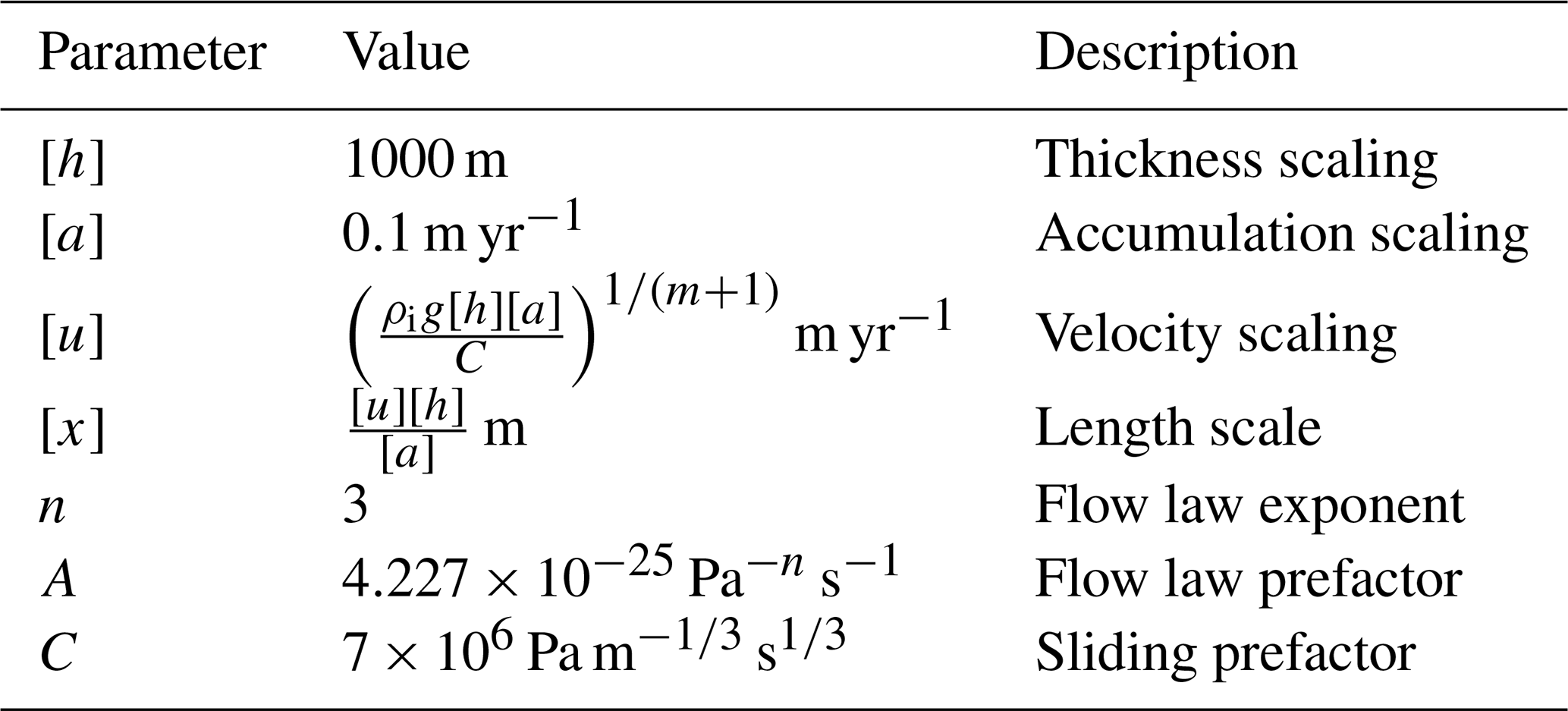
To understand the characteristic timescales of damage evolution, we nondimensionalize a one-dimensional (1D) form of Eq. (1), based on the following scalings:

$$\begin{array}{}\text{(2a)}& {\displaystyle }t=\left[t\right]t^{*},\text{(2b)}& {\displaystyle }u=\left[u\right]u^{*},\text{(2c)}& {\displaystyle }h=\left[h\right]h^{*},\text{(2d)}& {\displaystyle }D=D^{*},\text{(2e)}& {\displaystyle }f=\left[f\right]f^{*},\end{array}$$

wherein t is time, u is velocity, h is ice thickness, D is damage, and f is the damage evolution function in Eq. (1). Brackets denote the scaling for each parameter, and the asterisk denotes the nondimensionalization of each parameter. Using these scalings, we can rewrite Eq. (1) in 1D as

$$\begin{array}{}\text{(3)}& {\displaystyle \frac{\mathrm{1}}{\left[t_{\mathrm{a}}\right]}}{\displaystyle \frac{\partial D^{*}}{\partial t^{*}}}+{\displaystyle \frac{\left[u\right]}{\left[x\right]}}{u}^{*}{\displaystyle \frac{\partial D^{*}}{\partial x^{*}}}=\left\{\begin{array}{ll}\left[f\right]f^{*},& \left[\mathit{\sigma }\right]{\mathit{\sigma }}^{†*}\ge \left[\mathit{\sigma }\right]{\mathit{\sigma }}_{\mathrm{t}}^{*}\\ \mathrm{0},& \left[\mathit{\sigma }\right]{\mathit{\sigma }}^{†*}<\left[\mathit{\sigma }\right]{\mathit{\sigma }}_{\mathrm{t}}^{*}\end{array}\right.,\end{array}$$

where the timescale of the flow problem is the advective timescale $\left[t_{\mathrm{a}}\right]=\left[x\right]/\left[u\right]$. As this problem is simplified to the advection equation with no source/sink in the case of $\left[\mathit{\sigma }\right]{\mathit{\sigma }}^{†*}<\left[\mathit{\sigma }\right]{\mathit{\sigma }}_{\mathrm{t}}^{*}$, for the remainder of this derivation, we drop this case and focus on the case in which damage accumulates. Simplifying Eq. (3), we arrive at

$$\begin{array}{}\text{(4)}& {\displaystyle \frac{\partial D^{*}}{\partial t^{*}}}+u^{*}{\displaystyle \frac{\partial D^{*}}{\partial x^{*}}}=\left[t_{\mathrm{a}}\right]\left[f\right]f^{*}.\end{array}$$

The unit of [f] is inverse time. Therefore, we can identify a nondimensional number,

$$\begin{array}{}\text{(5)}& \mathit{\delta }=\left[t_{\mathrm{a}}\right]\left[f\right].\end{array}$$

This nondimensional number δ can physically be interpreted as a ratio of timescales: [t_a] is the advective timescale, and $\left[t_{\mathrm{f}}\right]=\frac{\mathrm{1}}{\left[f\right]}$ is a fracture timescale, describing the timescale at which fractures initiate, grow, and coalesce. The fracture timescale depends solely on the damage evolution function f, which is defined by the individual damage model. Using Eq. (4), when the rate of damage production is much greater than the advection rate, δ is large (δ>>1), and the advective timescale is far longer than the fracture timescale. When the rate of damage production is much less than the rate of advection, δ is small (δ≪1). Therefore, the magnitude of δ is a key parameter that dictates whether damage accumulates very rapidly compared to the flow model time step or whether damage accumulates on a similar timescale to the flow model. We hypothesize that, for most typical damage models and ice flow timescales, δ>>1; therefore damage accumulates faster than the flow timescale. This hypothesis is evaluated in the next subsection.

2.2 Flowline model coupled to damage model

To demonstrate the rapid rate of fracture within ice flow models, we couple a continuum damage mechanics model to a marine-terminating glacier flowline model. In the flowline model, the glacier terminates at the grounding line. The model solves the nondimensionalized shallow-shelf approximation momentum and mass balance equations in one-dimensional space, as in Schoof (2007), with an implicit numerical scheme for velocity, thickness, and grounding line position, following a Weertman sliding law with an exponent of m=3 (Weertman, 1957) and power-law rheology with an exponent of n=3 (Glen, 1955). The bed is a linear function of the length of the glacier, and the bed slope is prograde. The scales and relevant parameters used in the nondimensionalized flowline model and damage model are found in Table 1, and the full model equations can be found in the Supplement (Sect. S1). The numerical scheme, following Schoof (2007), is available through an open-source repository (link in Robel, 2021) and was previously applied in Robel et al. (2018) and Christian et al. (2022). To run this coupled model, we initialize the coupled flow–damage simulation from a steady glacier length of ∼450 km and zero damage, and we evolve flow and damage together.

Table 1 Scaling for the damage evolution model and flowline model.

Damage influences flow by the hypothesis of strain-rate equivalence, which states that, if a damaged material produces a strain-rate response under an applied stress, then the same material with no damage produces the same strain rate under an effective stress, which can be defined as $\stackrel{\mathrm{̃}}{\mathit{\sigma }}={\displaystyle \frac{\mathit{\sigma }}{\mathrm{1}-D}}$ (Lemaitre, 1985; Pralong and Funk, 2005). This is equivalent to introducing a scaling applied to the flow law prefactor $\stackrel{\mathrm{̃}}{A}=A(\mathrm{1}-\stackrel{\mathrm{‾}}{D}{)}^{-n}$, where $\stackrel{\mathrm{‾}}{D}$ is the depth-averaged damage and n is the viscous stress exponent, typically set to n=3 (Glen, 1955; Cuffey and Paterson, 2010).

Damage is solved explicitly using velocity and thickness fields. In this implementation, the velocity and thickness are solved with the depth-averaged damage field $\stackrel{\mathrm{‾}}{D}$ from the previous time step. To prevent the rate factor from becoming infinite, the maximum value of $\stackrel{\mathrm{‾}}{D}$ is set to D_max=0.99 rather than D_max=1. The damage increment at the current time step is then calculated from the velocity and thickness at the current time step. Further details of the numerical scheme can be found in Sect. S1.

We couple this flowline model to a CDM model. Equation (1) describes the general form of most CDM models, with an arbitrary damage evolution function f. Ultimately, the nature of the damage evolution function depends strongly on the specific physics of fracture mechanics represented in the model; therefore the damage evolution function varies widely amongst damage models applied to ice sheets. In the coupling of the flowline model, we use the damage model proposed by Pralong and Funk (2005) for simulating glacier calving. The damage evolution function in this model was initially proposed by Kachanov (1958) and Rabotnov (1968) to describe the time-dependent accumulation of damage as a kinetic process, which occurs during the tertiary creep stage of polycrystalline metals at high homologous temperatures. Thus, it was not intended to model specific fracture processes in ice sheets, as in Bassis and Ma (2015) and Sun et al. (2017), but rather to describe the bulk accumulation of creep damage in a representative material volume (Murakami and Ohno, 1981). A simplified version of this creep damage model uses a power-law damage evolution function as follows:

$$\begin{array}{}\text{(6)}& f=B({\stackrel{\mathrm{̃}}{\mathit{\sigma }}}^{†}-{\mathit{\sigma }}_{\mathrm{t}}{)}^r(\mathrm{1}-D{)}^{-k},\end{array}$$

where B is a damage rate factor, r and k are exponents, and ${\stackrel{\mathrm{̃}}{\mathit{\sigma }}}^{†}$ is the chosen invariant of the effective stress tensor. The dimensionless parameter δ can be written as

$$\begin{array}{}\text{(7)}& \mathit{\delta }={\displaystyle \frac{\left[x\right]}{\left[u\right]}}B[\stackrel{\mathrm{̃}}{\mathit{\sigma }}{]}^r.\end{array}$$

The values for B and r are taken from experimental constraints to be $B=\mathrm{5.23}\times {\mathrm{10}}^{-\mathrm{7}}$ MPa^−r s⁻¹ and r=0.43 (Duddu and Waisman, 2012, 2013a). To calculate stress for this continuum damage mechanics model, we extend the mesh at each grid point into the z direction to capture depth-varying damage. This has been determined to be necessary for the accurate representation of damage, particularly due to the effect of overburden pressure closing cracks (Keller and Hutter, 2014). Our method for calculating depth-varying stresses notably differs from that of Keller and Hutter (2014) in that we do not account for basal water pressure, which may allow basal crevasses. Thus, the damage we estimate is purely surface damage. We explore the potential effects of incorporating basal crevassing in the Discussion. The stress criterion we use for damage accumulation is the maximum (tensile) principal stress criterion σ₁≥σ_t. The scaling to nondimensionalize stress is based on the flow law (Glen, 1955):

$$\begin{array}{}\text{(8)}& \left[\mathit{\sigma }\right]=\mathrm{2}{\stackrel{\mathrm{̃}}{A}}^{-\frac{\mathrm{1}}{n}}({\displaystyle \frac{\left[u\right]}{\left[x\right]}}{)}^{\mathrm{1}/n}.\end{array}$$

We set the stress threshold for damage accumulation as σ_t=0.02 MPa, an arbitrary value for the purposes of evaluating the timescales of damage accumulation. This value is lower than expected in natural glaciers and ice sheets because the flowline model in this idealized geometry produces relatively low stresses; therefore this value must be set low to produce damage. Because the goal of this section is to evaluate the importance of the rate of damage accumulation, the specific value of the stress threshold should not significantly affect these results. We further investigate the importance of the stress threshold value in a two-dimensional (2D) geometry later in this paper.

With these parameters and those specified in Table 1, the dimensionless parameter δ is 7.83×10³, with an advective timescale of ∼10⁴ years and a fracture timescale of ∼1.3 years. The fracture timescale is significantly smaller than the advective timescale, as hypothesized. We would thus predict that fractures accumulate much more rapidly than they are advected by ice flow.

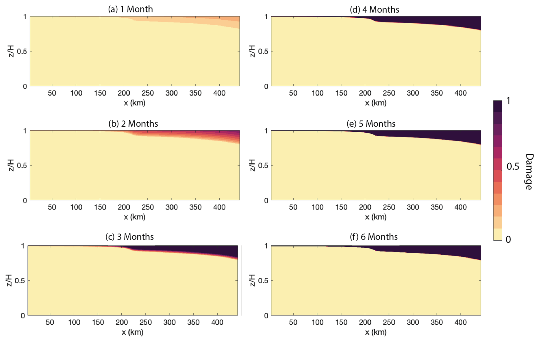
Figure 1 Damage evolution in a flowline model over 6 months: damage fields from the coupled flowline–damage model with a time step of 1 month for the first 6 months of the simulation. The flow moves from left to right, where the far-right boundary is the grounding line and terminus position of the glacier and the far left boundary is the inflow boundary. The simulation initializes with zero damage and at a steady-state position. Damage accumulates to D→1 everywhere where stresses are high enough for damage to initiate within the 6-month period of the simulation.

We evolve damage and flow with time steps of 1 month (Fig. 1). Damage is produced in all regions where the maximum Cauchy principal stress σ₁ equals or exceeds the stress threshold σ_t. The maximum Cauchy principal stress is equal to the longitudinal deviatoric stress minus the overburden pressure, which is a function of the vertical position in the glacier z. In this simulation, damage accumulates, as expected, primarily at the surface in the downstream region of the glacier, due to high deviatoric stresses and low overburden pressure in that region. Within 1 month, D≈0.2 accumulates near the surface (Fig. 1a). Damage continues to accumulate each month until it reaches D=1 everywhere where the stresses are large enough for damage to initiate. This occurs within 6 months (Fig. 1f). This agrees with the theory that, where δ>>1, fractures accumulate much more rapidly than they are advected away by ice flow. The implication of this is that the timescale from damage initiation to saturation (D≈1) is on the order of months, and explicitly simulating this short transient growth timescale has little effect on ice flow, which integrates the effects of D on the effective viscosity over timescales of decades to millennia. This is shown explicitly in the next two sections.

2.3 Diagnostic damage model

Given the speed at which damage reaches its maximum, we propose a diagnostic damage model, which is valid in the cases where δ is large and thus where the fracture timescale is much less than the advective timescale. This diagnostic model has three steps. (1) The model identifies regions where the chosen invariant of the effective Cauchy stress tensor ${\stackrel{\mathrm{̃}}{\mathit{\sigma }}}^{†}$ meets or exceeds the stress threshold σ_t, and it sets those regions of the domain to D=1, as in

$$\begin{array}{}\text{(9)}& D_{\mathrm{acc}}=\left\{\begin{array}{ll}\mathrm{1},& {\stackrel{\mathrm{̃}}{\mathit{\sigma }}}^{†}\ge {\mathit{\sigma }}_{\mathrm{t}}\\ \mathrm{0},& {\stackrel{\mathrm{̃}}{\mathit{\sigma }}}^{†}<{\mathit{\sigma }}_{\mathrm{t}}\end{array}\right..\end{array}$$

Using D_acc (Eq. 9), we find the depth-averaged damage ${\stackrel{\mathrm{‾}}{D}}_{{\mathrm{acc}}_i}$, where i denotes the current model time step, by enforcing the condition that depth-averaged damage cannot exceed some maximum value D_max (Eq. 10a). This step accounts for the rapid accumulation of damage in regions where the stress exceeds the threshold for damage initiation. (2) The model advects the depth-averaged damage field from the previous time step ${\stackrel{\mathrm{‾}}{D}}_{i-\mathrm{1}}$ using a transport equation with no source/sink term (Eq. 10b) to produce a damage field ${\stackrel{\mathrm{‾}}{D}}_{i-\mathrm{1}}^{+}$, where + denotes the solution of the advection equation at the current model time step of the damage field from time step i−1. This step allows the advection of damaged ice into regions that otherwise would not initiate damage. (3) The model calculates the final damage field by taking the maximum of ${\stackrel{\mathrm{‾}}{D}}_{{\mathrm{acc}}_i}$ and ${\stackrel{\mathrm{‾}}{D}}_{i-\mathrm{1}}^{+}$ (Eq. 10c).

$$\begin{array}{}\text{(10a)}& {\displaystyle }{\stackrel{\mathrm{‾}}{D}}_{{\mathrm{acc}}_i}=\min [{\stackrel{\mathrm{‾}}{D}}_{{\mathrm{acc}}_i},D_{\max }]\text{(10b)}& {\displaystyle \frac{\partial {\stackrel{\mathrm{‾}}{D}}_{i-\mathrm{1}}^{+}}{\partial t}}+\mathbf{u}\cdot \mathrm{\nabla }{\stackrel{\mathrm{‾}}{D}}_{i-\mathrm{1}}^{+}=\mathrm{0}\text{(10c)}& {\displaystyle }{\stackrel{\mathrm{‾}}{D}}_i=\max [{\stackrel{\mathrm{‾}}{D}}_{{\mathrm{acc}}_i},{\stackrel{\mathrm{‾}}{D}}_{i-\mathrm{1}}^{+}]\end{array}$$

The goal of this diagnostic damage model (Eq. 10c) is to represent the effect of damage on ice rheology and thus projections of flow changes and mass loss through flow acceleration. This model cannot represent damage for the purpose of modeling calving or rift propagation in ice sheets because such a goal would require small-timescale and small-spatial-scale representation of fracture propagation and interactions with the local stress field. For the purposes of studying the effects of damage on ice viscosity and ice flow, this diagnostic damage model simplifies the problem of evolving damage in flow models by reducing the free parameters in the damage problem to a single uncertain parameter: the stress threshold, along with the relevant form of the stress invariant dictating damage initiation.

This model is valid only for specific advective and fracture timescales for which δ is large. Figure 2a shows the parameter space of δ for varying advective timescales and fracture timescales. The fracture timescale used for the remainder of this study is denoted in Fig. 2 by the green dot. In these limits, δ varies from ∼10 to ∼10⁶, with delta increasing along a diagonal such that δ is large for large advective timescales and small fracture timescales. To show the range of values of δ for which this diagnostic damage model replicates full damage models, we compare the diagnostic damage model to the transient model of Pralong and Funk (2005) after 1000 model years for the range of δ values in Fig. 2a. We calculate the percentage difference in grounding line position (scaled by the total change in transient model grounding line position) after 1000 years. The difference in grounding line position is small (∼1 %–2 %) for δ larger than approximately 10³ and increases nonlinearly for δ<10³ (Fig. 2b). The results in Fig. 2 are shown in fracture and flow timescales generally, meaning any damage evolution function can be evaluated for timescale to determine whether this diagnostic model is applicable. If we assume a power-law form of the damage evolution function, as in Pralong and Funk (2005), Fig. 2 can be understood as evaluating the effect of varying power-law parameters, such as the damage rate factor B and the exponent r, on the applicability of the diagnostic damage model. That is, when the damage rate factor B is small, damage accumulates slowly and the diagnostic model is less likely to be applicable. This theory is largely insensitive to the choice for the stress threshold σ_t, as the stress threshold dictates where damage accumulates, but the rate of accumulation is controlled primarily by the values for B and r. In the Supplement (Fig. S1), we show that we obtain approximately the same parameter space using a larger value for the stress threshold.

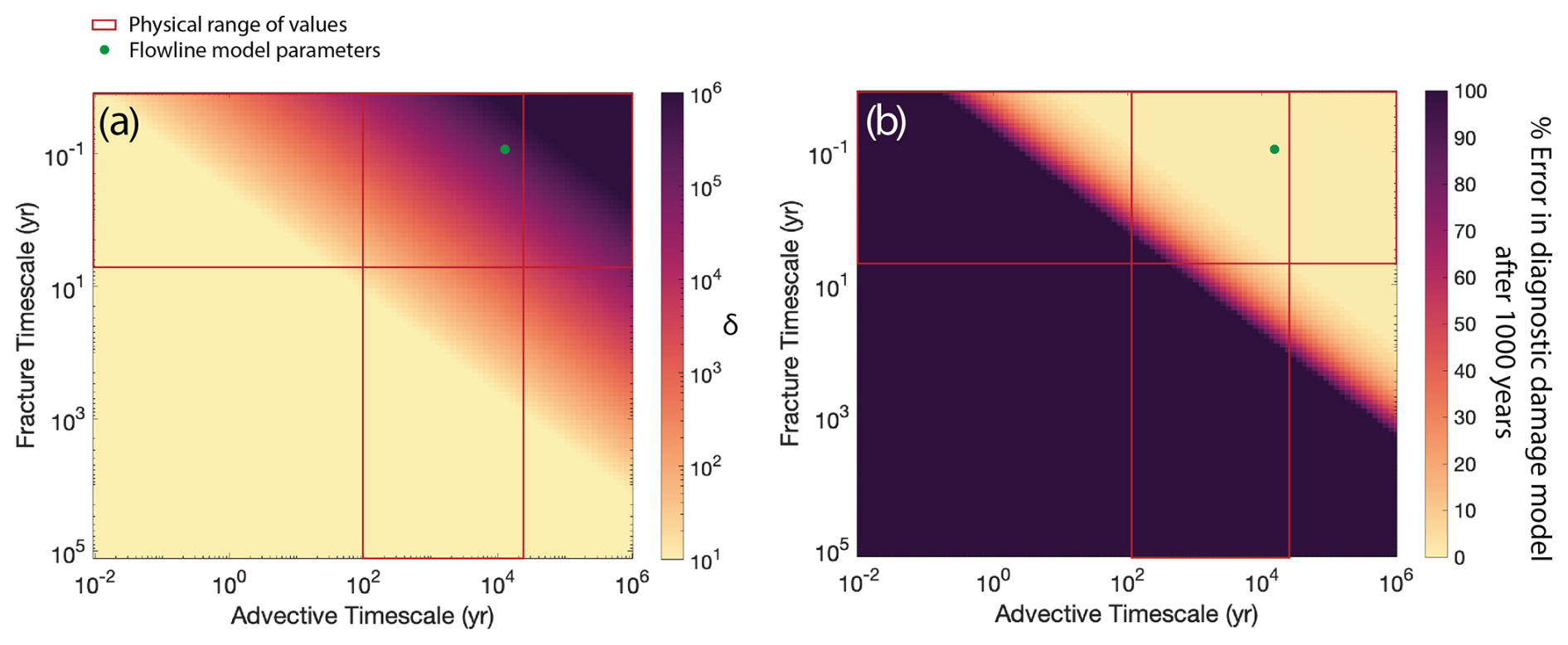
Figure 2 Timescales for which the diagnostic damage model is applicable: parameter space of fracture timescale and advective timescale for (a) nondimensional parameter δ (Eq. 7) and (b) the error in the grounding line position using the diagnostic damage solver (the difference between grounding line position found from coupling the flowline model with the transient damage model of Pralong and Funk (2005) and the grounding line position found from coupling the flowline model with the diagnostic damage model, scaled by the total grounding line change in the transient model) after a simulation time of 1000 years. The red box represents the likely range of values of advective and fracture timescales based on the geometry of ice streams and the physics of fracture, and the green dot denotes the parameters used in the flowline model.

2.4 Errors in the diagnostic damage model on long timescales

To demonstrate the accuracy of the diagnostic damage model (as compared to the full transient model) for longer glacier simulations, we compare the flow behavior using the diagnostic model and the full transient damage model. We initialize the flowline model with a steady-state model configuration, and then we turn on damage coupling and evolve the model to a new steady state. We do so for different climate forcing simulations, as climate forcing can vary on timescales much smaller than the advective timescale.

We first test a case without climate forcing (Fig. 3a), evolving the glacier state over 10 000 years. Both damage simulations produce a significant grounding line retreat of ∼6 % of the initial glacier length, with the control simulation (“No Damage”) producing no change as the model is initialized at a steady state. The diagnostic model replicates the transient model behavior well (Fig. 3a,ii), with the difference in the grounding line position not exceeding 1 % of the deviation from the initial state (Fig. 3a,iii).

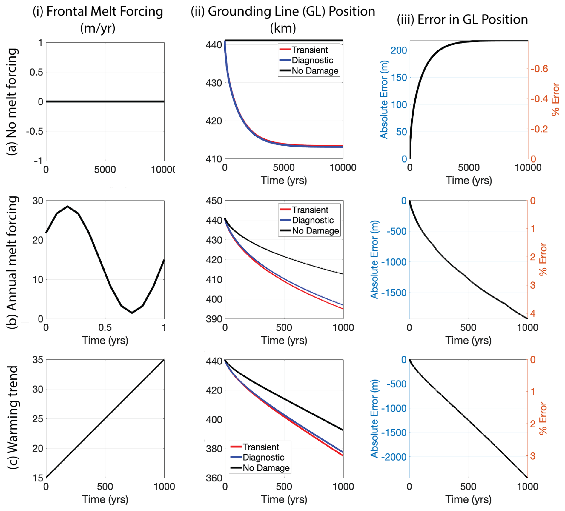
Figure 3 Comparison between 1D transient and diagnostic damage models: we run three different model simulations using no damage coupling, the full transient damage model of Pralong and Funk (2005), and the diagnostic damage model presented in Eq. (10c). We also present the grounding line position (ii) and the difference in grounding line position between the diagnostic damage model and the transient damage model (iii), including the difference in grounding line position as a percent of the amount of grounding line retreat by the transient model. (a) No climate forcing, in which the model is run for 10 000 years, during which the idealized glacier retreats for the cases of damage coupled with the transient model and the diagnostic damage model. The diagnostic damage model produces very little deviation from the full transient model. (b) Annual basal melt forcing, in which the model is run for 1000 years. The idealized model retreats in all cases, though it retreats faster and further in the case of damage coupling. (c) A warming climate in which basal melt forcing increases linearly over 1000 years. The diagnostic damage model again reproduces the transient behavior well, with errors <5 % of the amount of grounding line retreat from the transient model.

Next, we test the diagnostic damage model in a simulation with annual variations in frontal melt forcing over 1000 years (Fig. 3b). We define the following melt parameterization to simulate annual forcing:

$$\begin{array}{}\text{(11a)}& {\displaystyle }\dot{m}={\mathit{\mu }}_m+{\mathit{\eta }}_m,\text{(11b)}& {\displaystyle }{\mathit{\eta }}_m=M\sin \left({\displaystyle \frac{\mathrm{2}\mathit{\pi }t}{N}}\right),\end{array}$$

where μ_m is the mean melt rate, η_m is the melt rate anomaly, N is the period, M is the amplitude of forcing anomaly, and t is the time. We set μ_m=15 m yr⁻¹, N=1 year, and M=0.9μ_m (Fig. 3b,i). In all cases, incorporating damage produces more grounding line retreat than the control (“No Damage”) simulation, suggesting that, in this idealized setup, damage alters mass loss by acceleration of flow even when calving is not considered.

While the diagnostic damage model still produces roughly similar behavior to the full transient model (Fig. 3b,ii), the difference between the two models is larger than in the case without melt forcing (Fig. 3b,iii). However, the difference in grounding line position between the transient and diagnostic models remains under 5 % (<2000 m of grounding line position difference). Furthermore, most ice sheet simulations only run for a few centuries, in which case the differences in grounding line position remain between 2 %–3 %, well within other sources of uncertainty about the grounding line position.

The final case we test is one with a long-term warming trend, in which the melt rate increases linearly over the course of the run (Fig. 3c). In this case, we adjust Eq. (11a) to be

$$\begin{array}{}\text{(12)}& \dot{m}={\mathit{\mu }}_m+\mathrm{0.2}t,\end{array}$$

with t in years (Fig. 3c,i). The difference in grounding line position between the diagnostic damage model and the transient damage model is comparable to the case of annual melt forcing, with the error remaining below 4 % for the run of 1000 years (Fig. 3c,iii). In the Supplement (Fig. S2), we show other tests against interannual forcing, varying strength of the melt rate anomaly, and varying mean melt rate. Amongst all the runs, the diagnostic damage model replicates the transient behavior well, with grounding line position differences of just a few percent of the overall change from the initial steady state.

2.5 Reconciling the diagnostic damage model with other damage models in 2D

This diagnostic model has a similar basis to many existing physically based damage mechanics models. The two most widely applied damage mechanics approaches in glaciology include the power-law-based model of Pralong and Funk (2005) and the damage model based on the Nye zero-stress approximation. Here, we describe how the diagnostic damage model can reconcile both of these approaches and produce similar behavior in two-dimensional simulations.

The diagnostic damage model is expected to produce the same result as the continuum damage mechanics model applied in Pralong and Funk (2005), in the limit of the damage rate factor B→∞. Therefore, when B is significantly large, the diagnostic damage model approximates the result of the full Pralong and Funk (2005) model. The values of B and r for which this is true can be assessed calculating the resulting fracture timescale using Eq. (7). The parameter values for B and r used in this study are constrained from laboratory measurements in previous studies ($B=\mathrm{5.23}\times {\mathrm{10}}^{-\mathrm{7}}$ MPa^−r s⁻¹ and r=0.43) (Duddu and Waisman, 2012, 2013a). A similar comparison can be made for the strain-rate-based damage evolution function of Albrecht and Levermann (2012, 2014), in which the diagnostic damage model will approximate the full model for a sufficiently large γ, the damage accumulation rate factor.

The other approach used to model damage accumulation in glaciology builds on the Nye zero-stress approximation, in which surface crevasses will propagate to the depth at which the maximum principal deviatoric stress is balanced by the ice pressure (Nye, 1957; Benn et al., 2007a). This was extended to consider the depth at which basal crevasses will propagate as well (Nick et al., 2010), and this model framework has been applied in many ice damage modeling studies (Sun et al., 2017; Lhermitte et al., 2020; Kachuck et al., 2022). This approach estimates surface damage as

$$\begin{array}{}\text{(13)}& D_{\mathrm{s}}={\displaystyle \frac{{\mathit{\tau }}_{\mathrm{1}}}{p}},\end{array}$$

where D_s is surface damage (crevasse depth divided by ice thickness), τ₁ is the maximum principal deviatoric stress, and p is pressure. Implementations of the Nye zero-stress model define p=ρ_igh, where ρ_i is ice density, g is the gravitational constant, and h is ice thickness.

Similarly, the diagnostic damage model sets the damage value to maximum damage wherever a chosen invariant of the three-dimensional (3D) stress state exceeds a chosen threshold value. As a result, the damage accumulates to the depth at which

$$\begin{array}{}\text{(14)}& {\mathit{\sigma }}^{†}={\mathit{\sigma }}_{\mathrm{t}}.\end{array}$$

If we define ${\stackrel{\mathrm{̃}}{\mathit{\sigma }}}^{†}$ as the maximum principal stress σ₁, as is done in the implementation of the Nye zero-stress model, and if we define ζ as a scaled z coordinate such that ζ is 0 at the ice surface and 1 at the base of the ice, this can be rewritten as

$$\begin{array}{}\text{(15)}& {\displaystyle }{\mathit{\tau }}_{\mathrm{1}}-p\mathit{\zeta }={\mathit{\sigma }}_{\mathrm{t}}\text{(16)}& {\displaystyle }\Rightarrow \mathit{\zeta }={\displaystyle \frac{{\mathit{\tau }}_{\mathrm{1}}-{\mathit{\sigma }}_{\mathrm{t}}}{p}},\end{array}$$

in which σ_t is the stress threshold. Considering ζ is the depth to which damage propagates, ζ=D_s. Therefore, the Nye zero-stress model can be described as a case of this diagnostic damage model in which the stress threshold is the maximum principal stress and the stress threshold is zero.

To show that the diagnostic damage model replicates the Nye zero-stress model in the case of ${\mathit{\sigma }}^{†}={\mathit{\sigma }}_{\mathrm{1}}$ and σ_t=0 and that it also replicates the model of Pralong and Funk (2005) when using the parameter values constrained by experiments, we apply all three of these models to a benchmark glacier configuration used in the MISMIP+ experiments (Fig. 4c–e) (Asay-Davis et al., 2016). We use the open-source, Python-based ice sheet model icepack, which solves the shallow-shelf approximation of the momentum balance equations for glacier velocity (Shapero et al., 2021). The glacier is 640 km long and 80 km wide. The bed has a trough down the centerline, with the bed elevation higher in the margins (Fig. 4c). The mesh is refined in the vicinity of the grounding line to ∼1 km and is ∼4–6 km away from the grounding line. We apply a Weertman-style sliding law and a power-law rheology, with parameters prescribed by Asay-Davis et al. (2016), and we initially evolve the glacier to a steady state over 10 000 years. The steady-state ice thickness varies from ∼1500 m upstream to ∼300 m on the ice shelf (Fig. 4d). The glacier goes afloat (i.e., has a grounding line) approximately 460 km downstream in the centerline, and the glacier velocity increases sharply downstream of the grounding line, from <200 to >700 m yr⁻¹ (Fig. 4e).

We apply three different damage models: the Nye zero-stress implementation, the power-law implementation of Pralong and Funk (2005), and the proposed diagnostic damage model. We set the stress threshold to be σ_t=0 MPa and the stress criterion to be the maximum principal stress ${\mathit{\sigma }}^{†}={\mathit{\sigma }}_{\mathrm{1}}$. We only compare models for surface crevassing, not including the effects of basal crevasse production. While icepack solves the shallow-shelf equations in 2D, to calculate 3D damage as is done in the Pralong and Funk (2005) model and in the diagnostic damage model, we follow the workflow of Keller and Hutter (2014) and Huth et al. (2021b). We extrude the mesh and subsequently project the 2D velocity field onto the 3D mesh, solely for the calculation of the Cauchy stresses, and we then calculate damage in 3D.

The maximum value of 2D damage D_max ought to be set as close to 1 as possible, to simulate the complete loss of load-bearing ability of the ice. Due to challenges with numerical convergence of the velocity solver, however, D_max must be set to be some value less than 1 to avoid the loss of ellipticity when solving for the velocity field (D=1 implies effectively zero viscosity of ice and results in an undefined fluidity parameter as $\stackrel{\mathrm{̃}}{A}=A(\mathrm{1}-\stackrel{\mathrm{‾}}{D}{)}^{-n}$). Here, we set D_max≈0.8, which is the largest value for which we can consistently get numerical convergence. Because of the flow rate parameter's nonlinear dependence on D (viscosity $\propto (\mathrm{1}-D{)}^{-\mathrm{3}})$, the sensitivity of flow projections to D_max for values greater than D_max=0.5 in this MISMIP+ setup is quite small, as shown in the Supplement (Fig. S5). This may be because, for D_max=0.5, ice viscosity in the maximally damaged regions is sufficiently close to 0 to produce similar flow behavior to those with D_max>0.5 (that is, with a D_max=0.5, the maximum softening due to damage is a factor of 8). Previous work has shown that a similar value of D_max=0.86 replicates observations of Larsen C ice shelf rifting well by ensuring slow rift separation (Huth et al., 2023). However, it is presently unclear if the insensitivity to D_max is a robust behavior for all model geometries (e.g., Huth et al., 2023), so we recommend testing for D_max sensitivity in different model configurations.

From a steady state, which is reached with no damage coupling, we then couple each of the three models to flow by scaling $\stackrel{\mathrm{̃}}{A}=A(\mathrm{1}-D{)}^{-n}$ at each time step. The model is not forced with any melt or surface accumulation, so the results of this simulation are purely the effects of damage. Figure 4 shows the results of these three simulations.

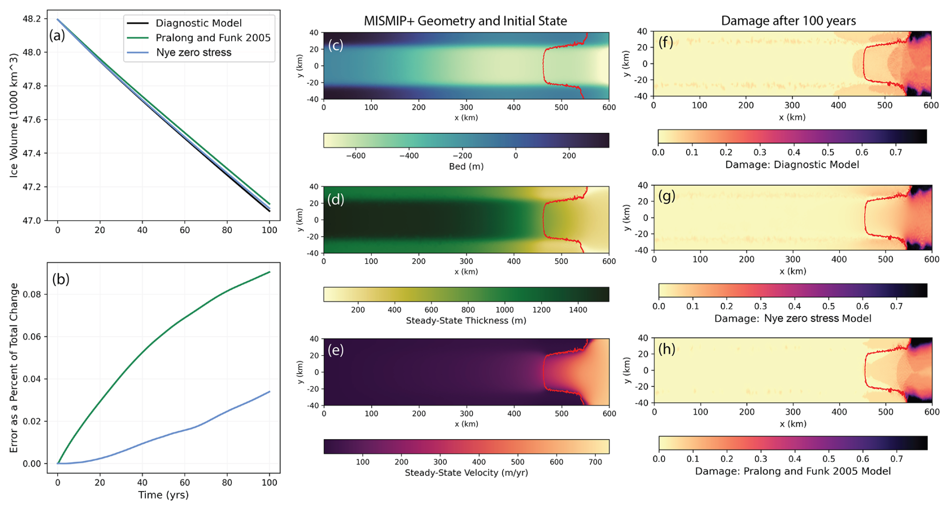
Figure 4 Comparison between 2D transient and diagnostic damage models. We set up a 2D model geometry as prescribed by the MISMIP+ configuration (Asay-Davis et al., 2016) and ran this from a steady state (c–e) without climate forcing and with couplings to three different damage models: the model of Pralong and Funk (2005), the Nye zero-stress model, and the diagnostic damage model proposed in this study. We refer to the Nye zero-stress model and the model of Pralong and Funk (2005) as “full” models. We show mass loss as estimated from each of these three models (a) and the differences between the full models and the diagnostic damage model (b). The difference is reported as the mass loss from the full model coupling minus the mass loss from the diagnostic damage model coupling, scaled by the total mass loss from the full model coupling. We show the final damage fields after 100 years for each of the three model couplings (f–h). The red line denotes the grounding line position.

All three models produce similar mass loss over the 100-year simulation (Fig. 4a), with the diagnostic damage model producing a deviation of less than 1 % from the Pralong and Funk (2005) model and the Nye zero-stress model (Fig. 4b). All three final damage fields also look very similar (Fig. 4f–h), with damage accumulating in the margins of the ice shelf and, to a lesser extent, in the centerline of the ice shelf and the margins of the grounded ice near the grounding line. The Nye zero-stress model produces a smoother damage field because it is in 2D, whereas, in the other two models, damage fields are calculated in 3D and depth-averaged. The three-dimensional approach of the diagnostic damage model allows more complex stress states to be considered when calculating fracture, as is done in the next section with the Hayhurst stress criterion.

Notably, none of these models include explicit healing processes in the form of damage sinks in the damage evolution equation, which is an assumption that may affect the validity of the diagnostic damage model. The only process preventing damage represented here is the effect of overburden pressure, which prevents cracks from propagating all the way through the ice thickness. The mechanisms of other healing processes are relatively uncertain, and many models do not include healing parameterizations due to uncertainty about the underlying physics and the form of the parameterization as applied to ice (e.g., Sun et al., 2017; Duddu et al., 2020; Huth et al., 2021b). The models that do include healing do so by defining an arbitrary healing rate and applying this to the stress or strain rate (Pralong and Funk, 2005; Albrecht and Levermann, 2012, 2014). Other models can result in a reduction in damage due to physical processes, such as viscous flow (Bassis and Ma, 2015). Though we do not include similar parameterizations here, we could accomplish a simple parameterization by reducing the damage at each time step by some fraction. Barring further physical intuition of experimental or observational data to inform the magnitude of healing, we leave the exploration of healing for future work. The estimates presented in this study, therefore, could be thought of as the upper bound on the effect of damage on flow.

3 Effect of damage on flow

We next seek to quantify the effects of damage and damage evolution on projections of future glacier behavior, along with the sensitivity of this coupled damage–flow model to the type of stress criterion and threshold, which are the primary degrees of freedom in the diagnostic damage model. To do so, we conduct the MISMIP+ experiment Ice1r, which simulates transient melt-driven grounding line retreat over 100 years. We initialize the model with the steady-state thickness and velocity fields, as shown in Fig. 4c–e, and initiate melt according to a depth-dependent melt parameterization prescribed by Asay-Davis et al. (2016) (Eq. 17; the melt field is shown in the Supplement).

$$\begin{array}{}\text{(17)}& \dot{m}=\mathrm{\Omega }\tanh {\displaystyle \frac{H_c}{H_{\mathrm{0}}}}max(z_{\mathrm{0}}-z_{\mathrm{d}},\mathrm{0}),\end{array}$$

where Ω is a free parameter that controls the magnitude of melting (Ω=0.2 yr⁻¹ as in Asay-Davis et al., 2016) and $H_c=z_{\mathrm{d}}-z_{\mathrm{b}}$ is the difference between the ice draft (thickness of the ice below the water level) z_d and the elevation of the bed z_b. We set H₀=75 m to be the reference thickness of the ice shelf cavity and $z_{\mathrm{0}}=-\mathrm{100}$ m to be the depth at which basal melting starts. Most of the melt is concentrated near the grounding line, with a maximum melt rate of ∼75 m yr⁻¹ a few tens of kilometers downstream of the grounding line, beyond which the melt rate tapers off to ∼10 m yr⁻¹. This melt forcing is applied at each model time step.

To account for multiaxial stresses, we apply the Hayhurst stress criterion to the diagnostic damage model, in agreement with previous work (Murakami and Ohno, 1981; Pralong and Funk, 2005; Jimenez et al., 2017; Huth et al., 2021b), defined as

$$\begin{array}{}\text{(18)}& \mathit{\chi }=\mathit{\alpha }\stackrel{\mathrm{̃}}{{\mathit{\sigma }}_{\mathrm{1}}}+\mathit{\beta }\sqrt{\mathrm{3}{\stackrel{\mathrm{̃}}{\mathit{\sigma }}}_{\mathrm{eq}}}+(\mathrm{1}-\mathit{\alpha }-\mathit{\beta })I_{\stackrel{\mathrm{̃}}{\mathit{\sigma }}},\end{array}$$

in which α and β are constant parameters, $\stackrel{\mathrm{̃}}{{\mathit{\sigma }}_{\mathrm{1}}}$ is the maximum principal value, ${\stackrel{\mathrm{̃}}{\mathit{\sigma }}}_{\mathrm{eq}}=\sqrt{\frac{\mathrm{1}}{\mathrm{2}}\stackrel{\mathrm{̃}}{\mathit{\sigma }}:\stackrel{\mathrm{̃}}{\mathit{\sigma }}}$ is the equivalent measure (the second invariant), and $I_{\stackrel{\mathrm{̃}}{\mathit{\sigma }}}$ is the trace (the first invariant) of the effective stress $\stackrel{\mathrm{̃}}{\mathit{\sigma }}$. Note that the second term in the Hayhurst stress is the effective von Mises stress scaled by β.

We find the effective stress ${\stackrel{\mathrm{̃}}{\mathit{\sigma }}}_{ij}\left(z\right)={\stackrel{\mathrm{̃}}{\mathit{\tau }}}_{ij}\left(z\right)-p\left(z\right){\mathit{\delta }}_{ij}$, where $\stackrel{\mathrm{̃}}{\mathit{\tau }}$ is the effective deviatoric stress tensor ($\stackrel{\mathrm{̃}}{\mathit{\tau }}=\mathit{\tau }/(\mathrm{1}-D)$) and p is ice pressure (Keller and Hutter, 2014). This definition assumes that hydrostatic stress is mostly compressive due to ice overburden pressure, so only the deviatoric stress should be rescaled by damage. To incorporate the effect of damage on pressure, we would need to apply a more sophisticated pressure boundary condition in the fully damaged elements corresponding to open rifts. We anticipate that this effect on flow rate would be less significant compared to its effect on local stress field. In the figures for the remainder of this paper, we present depth-averaged damage $\stackrel{\mathrm{‾}}{D}$, which is the field that is inserted into the flow solver in the next time step.

In this model setup, cracks are suppressed under high overburden pressure, so, in most of the regions where $\stackrel{\mathrm{‾}}{D}<D_{\max }$, the 3D damage field is non-zero only at the surface. Thus, we only capture surface crevassing, but we explore in the Discussion the potential effect of basal crevassing.

To implement the Hayhurst stress criterion, we take the values of parameters from Pralong and Funk (2005), which are determined based on uniaxial experiments by Mahrenholtz and Wu (1992), and we present the relevant parameters in Table 2. Unless otherwise denoted, we use a stress threshold of σ_t=0.1 MPa, in accordance with observational studies evaluating the stress threshold for fracturing in ice sheets (Vaughan, 1993; Grinsted et al., 2024; Wells-Moran et al., 2025). We depth-average damage for the purposes of inserting damage back into the depth-averaged velocity solver.

(Pralong and Funk, 2005)(Pralong and Funk, 2005)(Asay-Davis et al., 2016)(Asay-Davis et al., 2016)(Asay-Davis et al., 2016)(Asay-Davis et al., 2016)(Asay-Davis et al., 2016)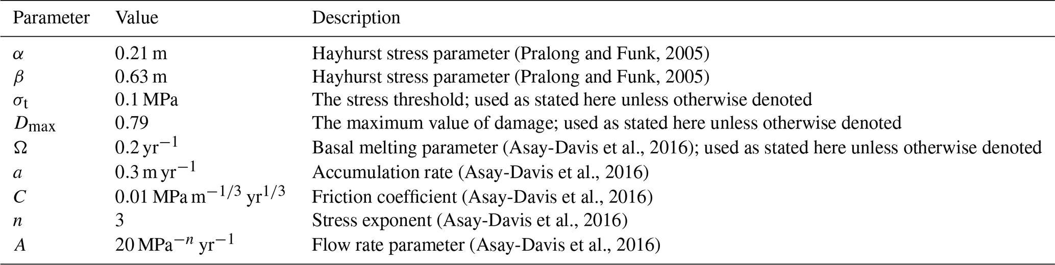

Table 2 Model parameters used in the MISMIP+ simulations.

In the remainder of this section, we seek to answer two questions: (1) what is the effect of initializing and evolving damage on the glacier flow response to forcing, compared to a control simulation where there is no damage in the model at all, and (2) what is the effect of evolving damage on this response to forcing, compared to a control simulation where damage is initialized (such as by an inverse method) but not evolved? We present two metrics for the response of the glacier to forcing and damage: ice volume loss, which is the difference in total ice volume from the beginning of the simulation to a given time step, and grounded area loss, which is the difference in the area of grounded ice from the beginning of the simulation to a given time step. In the subsequent sections, we present results from these two experiments.

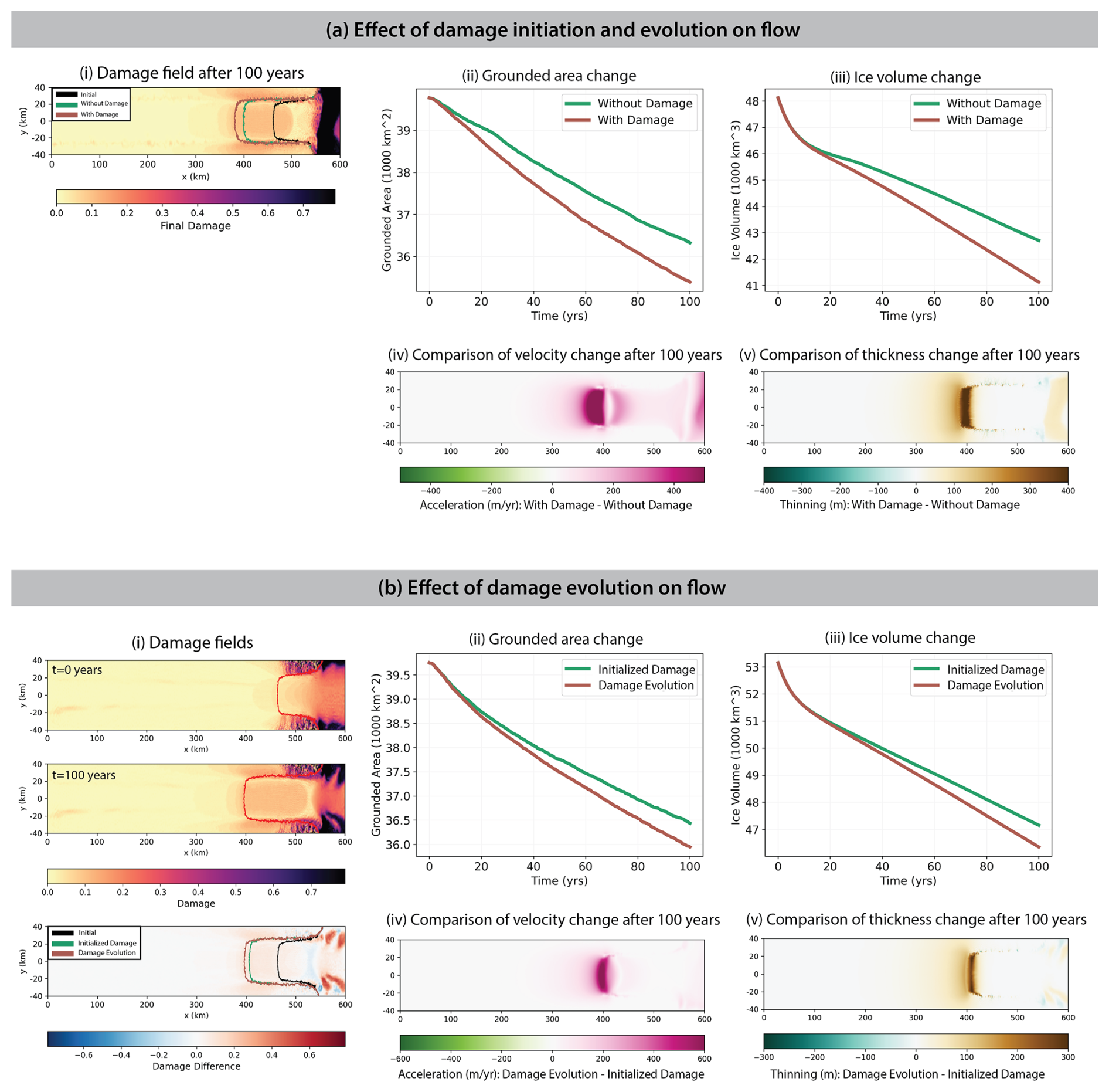
Figure 5 Effect of damage on glacier response to basal melt forcing. Results from a 100-year simulation of the MISMIP+ model configuration for two experiments: (a) evaluating the effect of damage initiation and evolution and (b) evaluating the effect of just damage evolution. We show (i) damage fields and grounding line change, (ii)–(iii) the effect on grounded area and ice volume, and (iv)–(v) the effect on change in ice velocity and thickness.

3.1 Impact of damage production and evolution

We initialize the glacier simulation according to Fig. 4c–e with zero initial damage, apply the melt rate beginning at t=0 from Eq. (17), and run the model for 100 years in two simulations. For the “Without Damage” simulation, damage is zero everywhere and does not change, and ice viscosity remains constant (as listed in Table 2) for the 100 model years. For the “With Damage” simulation, beginning at time t=0, damage is calculated by the diagnostic damage model (Eq. 10c) at every model time step, and this damage is used to calculate ice viscosity in accordance with the strain rate equivalence hypothesis $\stackrel{\mathrm{̃}}{A}=A(\mathrm{1}-D{)}^{-n}$. This is an input into the flow solver for the next time step.

Damage initiates in two regions of concentrated damage in the margins just downstream of the grounding line, primarily due to elevated shear stresses concentrated in the margins and tensile stresses in the center. Over 100 years, the lobes of damage on either margin extend towards the centerline, eventually connecting by t=100 years (Fig. 5a). The formation of this cross-glacier damaged region occurs for two reasons. Firstly, the melt rate under the center of the ice shelf thins the ice locally. Secondly, the ice pressure counteracting crack growth is defined as $p={\mathit{\rho }}_{\mathrm{i}}gh-{\mathit{\tau }}_{\mathrm{11}}-{\mathit{\tau }}_{\mathrm{22}}$, in which the horizontal normal stresses reduce the ice pressure and allow easier crack growth in the ice shelf center, as done in Keller and Hutter (2014) and Huth et al. (2021b). This cross-glacier damaged region is not seen in the similar simulations of Sun et al. (2017) and related studies, likely due to the exclusion of the normal stress terms in ice pressure.

The loss of load-bearing capacity in a continuous region across the ice shelf means that downstream ice transmits no buttressing stress upstream, thus representing the dynamic effect of calving on the remaining ice, even in the absence of explicitly simulated iceberg detachment. Some damage also accumulates in the margins near the grounding line and in the center of the ice shelf. In these regions, $\stackrel{\mathrm{‾}}{D}<\mathrm{0.2}$.

Including damage evolution in this model simulation causes both enhanced ice thinning and ice acceleration, concentrated around the regions of damage and the regions of maximum basal melting (Fig. 5a,iv–v). Ice accelerates primarily near the grounding line and towards the terminus of the glacier. There are also regions of acceleration in the trunk of the ice shelf. This aligns with the regions of maximum damage and also shows evidence of damaged regions downstream affecting flow upstream through decreased buttressing stress. Including damage causes the largest increase in acceleration of >400 m yr⁻¹ at the grounding line, where the flow is likely responding to a combination of local damage and the reduction in viscosity of the ice downstream on the ice shelf. The grounding line in the center of the ice shelf is also the region where damage contributes to thinning of the glacier, producing ∼400 m more thinning at the grounding line than the simulation without damage. The effect on glacier thinning extends approximately 100 km upstream of the grounding line across the glacier, including in the margins. This suggests a damage feedback that is induced by basal melting, in which basal melt triggers thinning of the ice shelf, which accelerates ice flow, which then produces damage via increased stresses, which itself accelerates flow. Given that the melt parameterization used here is a function of ice draft, the thinning of the ice shelf further concentrates the basal melting in the regions of thinning, which continue to produce more flow acceleration and damage production.

In response purely to melting without any damage (the control simulation), the grounding line retreats ∼75 km (Fig. 5a,i), a loss of 3400 km² of grounded ice area (Fig. 5a,ii) and 5400 km³ of total ice volume (Fig. 5a,iii). In response to melting along with damage initiation and evolution (“With Damage”), the grounding line retreats an additional ∼15 km, for a total retreat of approximately 90 km (Fig. 5a,i). The glacier loses 4400 km² of grounded ice area (Fig. 5a,ii) and 7000 km³ of total ice volume (Fig. 5iii). In this simulation, including damage leads to a roughly 29 % enhancement in ice volume loss from the no-damage simulation.

3.2 Impact of damage evolution

To isolate the effects of evolving damage, rather than the combined effects of initiating and evolving damage, we conduct a second experiment in which we spin up a new model steady state that includes damage. At the start of the experiment, there is an initial damaged field in both simulations (Fig. 5b,i). In this case, the “Initialized Damage” simulation calculates viscosity from this initial damage field, thereby initializing damage but not evolving damage as the stress field evolves in response to basal melt forcing. This approximates the standard approach in ice sheet modeling where ice viscosity is inferred from an observed velocity field (which presumably includes the effects of damage) through inverse methods, but then viscosity is then kept constant during the model run. For comparison, the “Damage Evolution” simulation initializes and evolves damage according to the diagnostic damage model (Eq. 10c).

In Fig. 5b,i, the steady state includes significant damage $(\stackrel{\mathrm{‾}}{D}\approx D_{\max })$ in the margins of the glacier just downstream of the grounding line and elevated damage in the center of the ice shelf, increasing towards the terminus of the glacier. Damage accumulates generally in the margins just downstream of the grounding line, where shear stresses are high, and then damage advects downstream. There are patchy regions of elevated damage in the margins near the grounding line on the grounded region of the glacier, but otherwise there is no damage on the grounded ice. After 100 years of damage evolution in response to basal melt forcing, the extensively damaged regions widen in the margins of the ice shelf. There is more damage ($\stackrel{\mathrm{‾}}{D}\le \mathrm{0.2}$) on the center of the ice shelf near the grounding line, extending over the grounding line to the grounded regions of the glacier. This is likely due to thinning that occurs in the center of the ice shelf due to the high basal melt rates in those regions (Fig. 5b,v), which reduces the effect of overburden pressure closing cracks. There are also lobes of low damage along the margins of the grounded glacier upstream from the patchy fractured regions. This is also likely due to the thinning that occurs in the margins around 350–425 km along the glacier (Fig. 5b,v).

Notably, there are minor asymmetries in the damage field, particularly at t=100 years. Given that the MISMIP+ geometry is symmetric and there are no asymmetries in the melt forcing field, it is possible that these asymmetries are either numerical artifacts, the result of an asymmetric mesh, or the result of physical symmetry breaking. The exact location of these damaged regions is not likely to have a significant effect on the rates of mass loss or grounding line change, and further reducing the time step, to avoid artificial diffusion in the numerical solution, does not affect the mass loss results (Fig. S4). Furthermore, there are numerical methods, such as the material point method previously used by Huth et al. (2021a, b, 2023), that may alleviate some numerical artifacts.

The simulation with damage evolution produces more acceleration in ice velocity at the grounding line (a difference of ∼500 m yr⁻¹) and more thinning (a difference of ∼400 m), aligning with the regions of maximum basal melting. There is minor development of damage at the surface ($\stackrel{\mathrm{‾}}{D}\sim \mathrm{0.1}$) in this region. Furthermore, the development of damage both in the center and in the margins of the ice shelf reduces its buttressing capacity, which can enhance ice velocity in the simulation with damage evolution.

In response to melting, in the “Initialized Damage” simulation, the glacier loses 3300 km² of grounded ice area (Fig. 5b,ii) and 6000 km³ of total ice volume (Fig. 5b,iii). In response to melting and damage evolution (“Damage Evolution”), the glacier loses 3800 km² of grounded ice area (Fig. 5b,ii) and 6800 km³ of total ice volume (Fig. 5b,iii), resulting in an ∼13 % enhancement of ice volume loss due solely to damage evolution. This suggests that initializing damage (either explicitly or implicitly by viscosity) at the start of a model run, for example, through the use of inverse methods (e.g., Borstad et al., 2013), does capture some of the damage effects but does not sufficiently replicate the evolving effects of damage in response to climate forcing.

3.3 Effect of uncertain parameters

A significant advantage of the diagnostic damage model is its simplicity. In particular, it reduces the number of free model parameters to one: the stress threshold, which encompasses both the specific value and the type of criterion used. However, there remains uncertainty about both the nature of the stress criterion and the value of the stress threshold. Here, we treat the type of stress criterion and the value of the stress threshold as uncertain model inputs and evaluate the effects of the choice of this stress threshold on projections of future flow (Figs. 6–7). We set up model simulations to study the effect of damage evolution, as in the previous section. To compare across different stress criteria (Fig. 6) and thresholds (Fig. 7), we report the percent enhancement of ice volume loss, which is the difference in the ice volume loss at each model year as a percent of the ice volume loss for the simulation with no damage evolution at that model year. It can be described as the percent increase in ice volume loss that can be attributed to evolving damage during the simulation.

Figure 6 Effect of damage on ice volume loss for varying stress criterion: results from a 100-year simulation for (b) the Hayhurst criterion, (c) the maximum principal stress criterion, and (d) the von Mises criterion. (a) We show the percent enhancement of ice volume loss (difference in ice volume loss between a simulation with damage evolution and a simulation with damage initialization but no evolution as a percentage of total ice volume loss in the damage initialization simulation) and the damage fields (the initial and final damage and the total damage change).

We first evaluate the effect of the stress criterion on future flow behavior (Fig. 6). We explore three stress criteria applied or studied in ice sheets previously: the von Mises stress, which describes the yielding of ductile materials (e.g., Albrecht and Levermann, 2012, 2014; Choi et al., 2018, 2021); the Hayhurst stress, as described previously (e.g., Pralong and Funk, 2005; Keller and Hutter, 2014; Mobasher et al., 2016; Jimenez et al., 2017; Huth et al., 2021b, 2023); and the maximum principal stress. In conducting this comparison, we use a value of D_max=0.5 for numerical stability, as the von Mises criterion produces such extensive damage that the flow solver cannot converge with a larger value. We evaluate these three criteria using the same stress threshold value of σ_t=0.1 MPa. The von Mises stress criterion produces extensive full-thickness damage in its steady state across the ice shelf and near the grounding line on the grounded regions. There is also damage extending fully upstream in the glacier. As the glacier responds to basal melt forcing, the full-thickness damage continues to accumulate through the grounded ice regions. There is significant grounding line retreat in response to basal melting, with damage evolution producing far more grounding line retreat than without damage evolution. This is because the von Mises criterion is based on deviatoric stresses, rather than Cauchy stresses; thus it does not incorporate the effect of pressure preventing the propagation of cracks. Using the von Mises stress criterion with damage evolution produces an ∼33 % enhancement in ice volume loss compared to the “Initialized Damage” simulation. The maximum (most tensile) principal stress criterion produces the least enhancement to ice volume loss (∼11 %) compared to the simulation with no damage evolution. In this case, the damaged regions are concentrated on the ice shelf, primarily in the margins. Finally, the Hayhurst criterion produces an ∼14 % enhancement in ice volume loss by 100 model years.

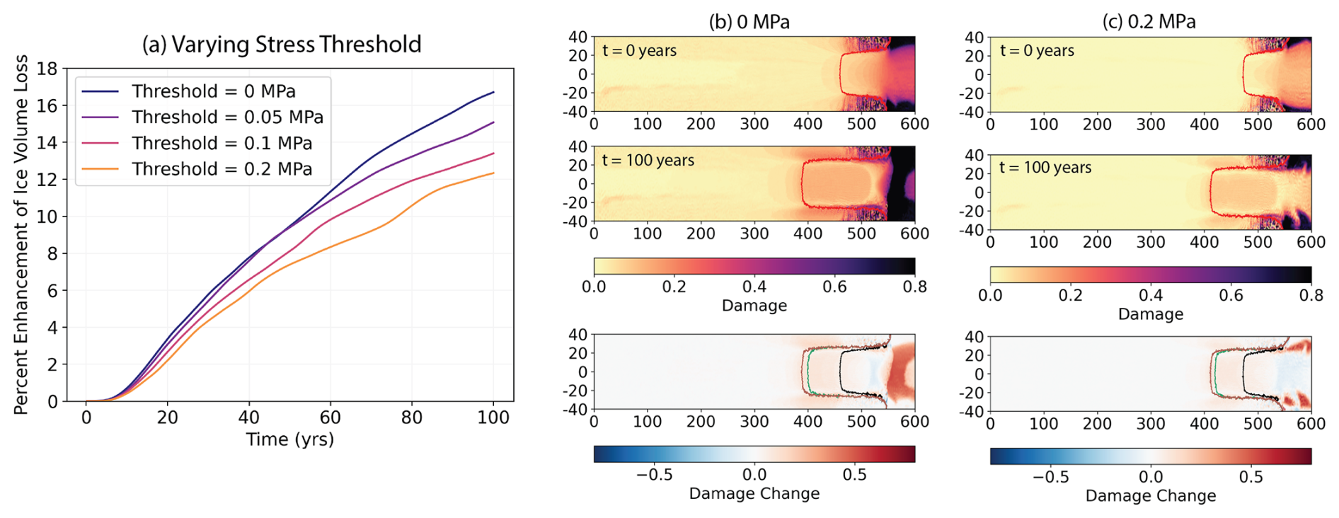
Figure 7 Effect of damage on ice volume loss for varying stress threshold: results from a 100-year simulation for ${\mathit{\sigma }}_{\mathrm{t}}=\mathrm{0},\mathrm{0.2}$ MPa. We show (a) the percent enhancement of ice volume loss (difference in ice volume loss between a simulation with damage evolution and a simulation with damage initialization but no evolution as a percentage of total ice volume loss in the damage initialization simulation) and (b–c) the damage fields (the initial and final damage and the total damage change) for ${\mathit{\sigma }}_{\mathrm{t}}=\mathrm{0},\mathrm{0.2}$ MPa.

We next evaluate the effect of the choice of stress threshold σ_t (Fig. 7). Varying the stress threshold produces less variation in the ice volume loss enhancement. We treat σ_t=0 MPa as an upper bound on the potential effect of damage and note that this approximates a Nye zero-stress model for fracture evolution in ice sheets. As the threshold increases, both the initial steady-state damage field and the damage field after 100 years decrease, with the maximum damage concentrating in the margins. As the threshold decreases, the damage field after 100 years of basal melting increases in the center of the ice shelf near the terminus, and the full-thickness damaged regions in the margins thicken. Furthermore, as the stress threshold value decreases, the enhancement of ice volume loss due to damage evolution increases, from 10 % with σ_t=0.2 MPa to 13 % with σ_t=0.01 MPa. This suggests an uncertainty of only a few percent of ice volume loss enhancement due to uncertainty about the specific value of the stress threshold, over the explored range. There is not a significant difference in the ice volume enhancement between σ_t=0.05 MPa and σ_t=0.1 MPa, due to there being few regions of stress separating these two thresholds in the idealized model setup. We expect that, for a different model setup, there might be more of an enhancement for σ_t=0.05 MPa than for σ_t=0.1 MPa. The stress threshold cannot be smaller than 0 in the absence of compressional fracture processes. Therefore, the effect of damage on flow is bounded above, in this case at ∼14 % by 100 years.

4 Discussion

4.1 Magnitude of enhancement to flow due to damage

Based on the idealized simulations run with the benchmark MISMIP+ glacier geometry, we find that evolving damage enhances mass loss by ∼13 % compared to the simulation that initializes ice viscosity by damage but does not evolve damage. To contextualize the magnitude of ice loss enhancement, we compare this enhancement to that produced by increasing the climate forcing (in this case, the basal melt rate). We do so by varying the parameter Ω (as in Eq. 17) and running simulations to 100 years in which we initialize a damage field but do not evolve damage during the simulation. We compare these to a simulation in which we initialize and evolve a damage field with a basal melting rate computed using Ω=0.2 yr⁻¹ (Fig. 8). At year 100, the enhancement to ice loss and grounded area loss from damage evolution with Ω=0.2 yr⁻¹ is similar to increasing the rate of basal melt by 50 % in a simulation with no damage evolution. Basal melting causes a more immediate response in ice volume loss on timescales of 0–30 years, while the effect of damage increases more significantly between 40–100 years. Increased basal melting (Ω=0.3 yr⁻¹) and damage evolution with lower basal melting (Ω=0.2 yr⁻¹) have the same response to grounded area loss until approximately 60 years, at which point damage evolution produces slightly more grounded area loss (∼100 km² by year 100). Ultimately, these results highlight the significant effect that damage evolution may have on century-scale estimates of ice sheet change and provide motivation for the incorporation of a damage evolution model into large-scale ice sheet models.

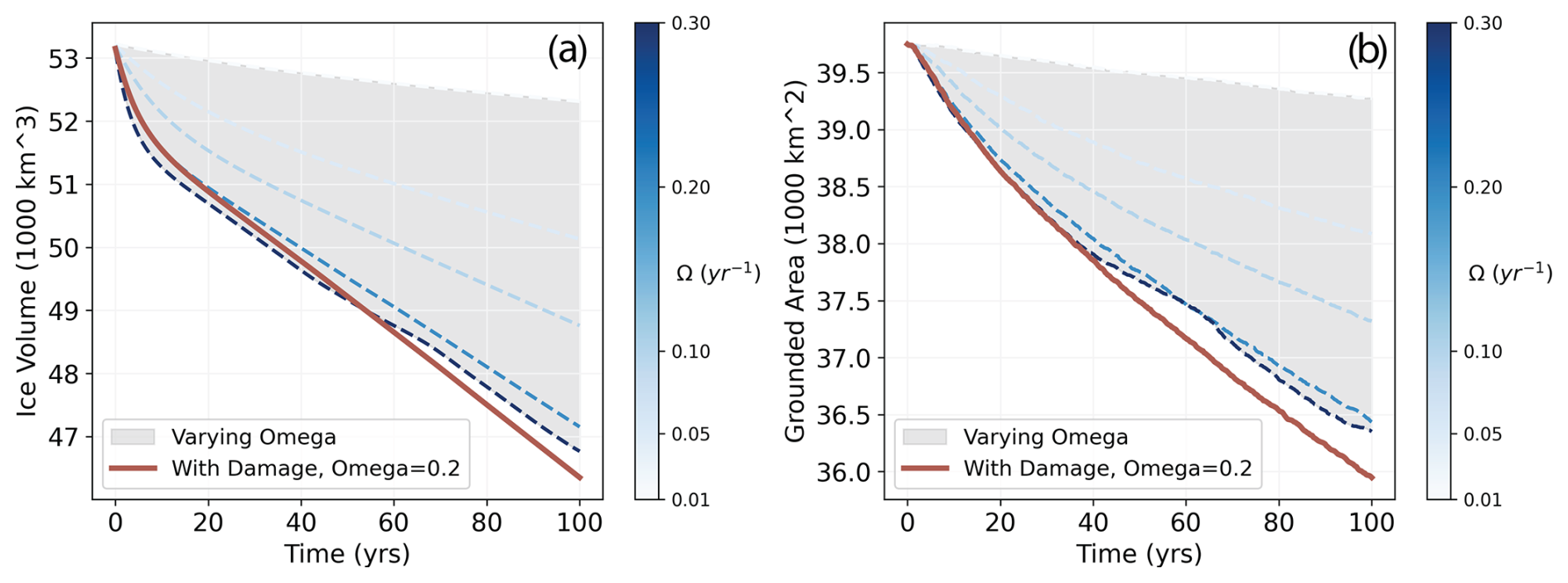
Figure 8 Comparing the effect of damage on flow with the effect of increased basal melt rate: results of (a) ice volume and (b) grounded area from 100-year simulations. The dashed blue lines show results from evolving the glacier in response to varying magnitudes of basal melting (in which the color of the line denotes the magnitude of basal melt forcing) with no damage. The red line shows a case with damage evolution and Ω=0.2 yr⁻¹.

4.2 Application of results to damage evolution in ice sheets

Many recent studies have presented observations of damage evolution in regions of the Antarctic Ice Sheet. Most notably, the southern margin of Pine Island Glacier in West Antarctica has accumulated significant damage over the last 2 decades (Lhermitte et al., 2020; Sun and Gudmundsson, 2023; Izeboud and Lhermitte, 2023). This damaged region initiates large-scale rifts that ultimately calve icebergs from the ice shelf (Lhermitte et al., 2020) and is correlated with a significant weakening (an increase in ice fluidity of approximately 2 orders of magnitude) in the shear margin and the outward movement of the shear margin (Sun and Gudmundsson, 2023). Similar damage evolution has occurred across the Thwaites Ice Shelf (Surawy-Stepney et al., 2023a; Izeboud and Lhermitte, 2023).

Our results here do not directly apply to the case of Pine Island Glacier, but we can provide insight into the processes occurring in the Amundsen Sea Embayment. In our idealized simulations, we identify similar weakening in the margins of the ice shelf and the initiation of maximally damaged regions that extend across the width of the ice shelf, representing a calving event. These simulations do not represent margin migration, but future simulations can be set up to determine the extent of future margin migration due to damage evolution. Furthermore, we provide evidence for a potential feedback between basal melting and damage evolution, in which basal melting causes thinning of an ice shelf, which enhances the spatial extent and the penetration depth of damage, which in turn enhances the thinning of the ice shelf. This is a feedback that may be taking place in these regions of the Amundsen Sea Embayment, such as Pine Island Glacier, where ocean warming is a primary driver of glacier change (Payne et al., 2004; Joughin et al., 2010). This may contribute to the processes driving damage evolution in the southern margin of Pine Island Glacier.

Finally, we identify the importance of constraining the stress criterion and stress threshold to reduce damage-induced uncertainty about future flow estimates. Studies have made progress on constraining parameters in damage models. In particular, improved spatial and temporal resolution of satellite observations have enabled more high-resolution and reliable maps of fracture and damage fields across the Antarctic Ice Sheet (Vaughan, 1993; Hulbe et al., 2010; Lai et al., 2020; Izeboud and Lhermitte, 2023; Surawy-Stepney et al., 2023b; Grinsted et al., 2024; Wells-Moran et al., 2025). Since these fields are derived primarily from optical imagery of ice sheet surfaces, they are currently limited to damage extent on the surface. However, these observations can be used both to validate damage models and to provide insight into the values of σ_t and the stress criterion used in damage models. Such observations have been applied to constrain the stress criterion for glacier ice against crevasses in the Antarctic and Greenland ice sheets, and they find that the von Mises criterion produces a generally good fit to observed crevasses, along with other criteria not considered in this study (Vaughan, 1993; Grinsted et al., 2024; Wells-Moran et al., 2025). Further, numerous laboratory and observational studies have sought to quantify this value for ice, with laboratory estimates ranging from 800 kPa to 5 MPa (Currier and Schulson, 1982) and observational estimates ranging from 80 kPa to 1 MPa (Vaughan, 1993; Ultee et al., 2020; Grinsted et al., 2024; Wells-Moran et al., 2025).

4.3 Model assumptions and simplifications

We present and apply a novel diagnostic damage model in this study to evaluate the effect of damage on ice flow on long timescales. This model operates under the assumption that the timescales of ice flow are significantly longer than the timescales of ice fracture and that damage therefore accumulates rapidly compared to flow model time steps. This model is not applicable, however, to simulations of ice dynamic processes occurring on short timescales and is therefore inappropriate for representing calving events or rift propagation on ice shelves, which can occur on timescales much less than 1 year (De Rydt et al., 2018; Clerc et al., 2019; Cheng et al., 2021; Olinger et al., 2022; Surawy-Stepney et al., 2023a). Representing the coupled flow and fracture processes involved in rift initiation and propagation would require running transient damage mechanics and ice flow models on small time steps that can represent the rift behavior on fracture timescales. To ensure numerical stability and mesh independence, previous work has shown that this benefits from nonlocal damage models (Jimenez et al., 2017; Huth et al., 2023) and a small enough time step that damage accumulation does not exceed a set threshold value at each time step. Given these constraints on representing rift propagation, we suggest that the diagnostic damage model should mainly be used to model the effect of damage on long-term ice viscosity and flow evolution. There is still significant value in understanding and modeling the underlying mechanics of crack initiation and propagation on short timescales to answer other scientific questions, for example, the role of depth-varying ice material properties on crevasse propagation (Gao et al., 2023; Clayton et al., 2024).

Even for the modeling of long-term ice viscosity, there is a need for further research on the applicability of continuum damage mechanics models to damage projections. Previous studies have noted that evolving damage over long time steps can blur the sharpness of cracks or cause unrealistic crack propagation due to errors in the integration of the damage rate, which can result in unrealistically large regions of full-thickness damage (Huth et al., 2021b). Transient damage models that aim to capture sharp rifting prevent this by adapting the time step size so that changes in damage accumulation are sufficiently small over each time step to ensure accurate and numerically stable crack propagation (e.g., Huth et al., 2021b, 2023). Evaluation of mesh and time step dependence (Fig. S4) in this study has shown that, for the case of the MISMIP+ configuration, these issues likely do not affect the results presented here. However, for more complex glacier geometries and model configurations, there is a need for further examination of the time step and mesh dependence of long-timescale damage modeling.

The ice sheet model icepack uses the shallow-shelf approximation (SSA), which calculates depth-averaged flow fields. While this work does capture the effect of vertically varying ice pressure, as discussed in the next paragraph, this assumption still neglects some vertical complexity which may be especially important on grounded ice, as basal properties affect the vertically varying flow of ice. Future work may consider full three-dimensional stress and flow states in determining the effect on damage in ice, particularly as we consider the anisotropy of damage and tension-compression asymmetry in the effect of damage on viscosity. This assumption also precludes a representation of the vertical advection of damage. While there are significant uncertainties about the magnitudes of vertical velocities, which may make incorporating these effects challenging, future work may also consider the effect of vertical advection on damage at depth.

In this study, damage is estimated from 3D Cauchy stresses, which are found by taking the deviatoric stresses from the 2D flow model and subtracting the pressure from the overlying ice. Therefore, we are primarily modeling the effects of surface crevassing, since the surface is where the ice overburden pressure is small enough to open cracks. However, there are crevasses that open up at the bottom of ice shelves, as the seawater pressure counteracts some of the ice overburden pressure (Weertman, 1973; Van Der Veen, 1998a; Luckman et al., 2012; McGrath et al., 2012; Buck and Lai, 2021). A way of modeling this effect of water pressure is to calculate Cauchy stresses from the deviatoric stress subtracted by an effective pressure, computed as the difference between ice pressure and water pressure for all depths below sea level. This approach is outlined in Keller and Hutter (2014) and Huth et al. (2021b) and described further in Sect. S4. We show in Sect. S5 that using effective pressure to estimate damage produces damage that extends further in ice thickness, including full-thickness damage in the margins near the grounding line. However, there remain significant uncertainties about the depth variation in pressure. Most importantly, the estimation of stress here assumes an isothermal ice shelf, whereas, in Antarctic ice shelves, the temperature of the ice likely increases with depth. This has implications for the stress field and thus the potential for basal crevasses to open, as explored in Coffey et al. (2024). Therefore, we leave the exploration of basal damage and its effect on rheology and ice flow velocity for future work.

The diagnostic damage model assumes rapid damage accumulation but does not represent any processes that heal existing cracks or counteract the opening of cracks, with the exception of the effect of overburden pressure. A few ice damage models represent healing and typically assume an arbitrary rate of healing (Pralong and Funk, 2005; Albrecht and Levermann, 2012, 2014) due to a lack of physical understanding surrounding healing processes in ice. Studies on other polycrystalline solids have represented kinetic healing processes, describing healing due to the movement of atoms closer together, by defining an activation energy for crack formation and healing (e.g., Miao and Engr, 1995; Arson, 2020). Representing crack closure from overburden pressure by using three-dimensional Cauchy stresses is a different method of representing a similar mechanism, though it does not account for the effect of longitudinal, lateral, and shear deformation causing crack closure. Further work needs to be done to understand the speed and magnitude of these healing processes in counteracting damage accumulation.

5 Conclusions

In this study, we seek to quantify the effect of damage on long-term glacier flow behavior. We first show that, in viscous glacier flow models, damage can be modeled diagnostically, while damage accumulation on short timescales is not explicitly modeled. We then apply this diagnostic damage model to quantify the effect of damage on marine-terminating glacier response to climate forcing. We couple the diagnostic damage model to an ice flow model and force the idealized marine-terminating glacier with basal melting as in the MISMIP+ experiment Ice1r. We find that the reduction in ice viscosity due to damage that evolves during the simulation in response to the changing stress field enhances ice mass loss by ∼29 % compared to a simulation that does not consider the effect of damage on viscosity. We find that initializing ice viscosity by damage but not evolving damage in response to stress changes during the simulation captures some of this enhancement, but still evolving damage with flow produces an ∼13 % enhancement in mass loss compared to solely initializing damage. This result suggests that initializing ice viscosity through inversions of damage (as in Borstad et al., 2012) is necessary but not sufficient to capture the effects of damage on ice rheology.

The results of this work suggest that (1) the damage model presented here provides a simplified way of incorporating damage evolution into ice sheet models for the purposes of representing the effect of fracture on ice viscosity, as it does not require representation of specific fracture physics and reduces parametric uncertainty within the damage model, and that (2) incorporating the evolution of fractures across scales into ice viscosity is necessary to fully capture the effect of climate forcing on ice sheets on long timescales. However, there is still more to understand, from modeling, observational, and experimental perspectives, about the mechanisms of fracture accumulation and crack healing in order to represent fully the effect of damage on ice flow in these models. There is also a demonstrated need for future observational and experimental constraints on the fracture threshold and fracture criterion and for more observations of fractures across scales that can be used to benchmark damage models. The synthesis of such data with models that can represent the effects of damage on long-timescale ice flow will be a significant step towards improving the physical fidelity of ice sheet models.