Impacts of air fraction increase on Arctic sea ice density, freeboard, and thickness estimation during the melt season

Arctic sea ice has undergone significant changes over the past 50 years. Modern large-scale estimates of sea ice thickness and volume come from satellite observations. However, these estimates have limited accuracy, especially during the melt season, making it difficult to compare the Arctic sea ice state year to year. Uncertainties in sea ice density lead to high uncertainties in ice thickness retrieval from its freeboard. During the Multidisciplinary drifting Observatory for the Study of the Arctic Climate (MOSAiC) expedition, we observed a first-year ice (FYI) freeboard increase of 0.02 m, while its thickness decreased by 0.5 m during the Arctic melt season in June–July 2020. Over the same period, the FYI density decreased from 910 to 880 kg m⁻³, and the sea ice air fraction increased from 1 % to 6 %, due to air void expansion controlled by internal melt. This increase in air volume substantially affected FYI density and freeboard. Due to differences in sea ice thermodynamic state (such as salinity and temperature), the air volume expansion is less pronounced in second-year ice (SYI) and has a smaller impact on the density evolution of SYI and ridges. We validated our discrete measurements of FYI density from coring using co-located ice topography observations from underwater sonar and an airborne laser scanner. Despite decreasing ice thickness, a similar counterintuitive increasing ice freeboard was observed for the entire 0.9 km² MOSAiC ice floe, with a stronger freeboard increase for FYI than for less saline SYI. The surrounding 50 km² area experienced a slightly lower 0.01 m ice freeboard increase in July 2020, despite comparable 0.5 m melt rates obtained from ice mass balance buoys. The increasing sea ice air volume defines the rapid decrease in FYI density, complicates the retrieval of ice thickness from satellite altimeters during the melt season, and underlines the importance of considering air volume and density changes in retrieval algorithms.

1 Introduction

The ultimate goal of mass balance observations of Arctic sea ice is to produce reliable ice thickness measurements throughout the year. Unless sea ice thickness is directly measured using ice coring, ice mass balance buoys, or ground-based electromagnetic sounding, it relies on remote methods such as airborne or satellite laser (ICESat, ICESat-2) and radar (e.g., Sentinel-3, CryoSat-2) altimeters (Paul et al., 2018), airborne electromagnetic sounding (Haas et al., 1997), moored upward-looking sonars (Sumata et al., 2023), and sonars mounted on underwater vehicles (Lyon, 1961). Except for electromagnetic sounding, these remote techniques estimate either the snow or sea ice freeboard (elevation above the waterline) or the ice draft (elevation below the waterline). Converting draft or freeboard to sea ice thickness under the assumption of hydrostatic equilibrium requires information on the snow thickness and density of both snow and sea ice.

Sea ice and snow density, as well as snow thickness, play an important role in aerial and satellite altimetry (Dawson et al., 2022), but they are rarely if ever measured directly from remote platforms. Ice thickness estimates from altimetry often use constant ice density for certain ice types including first-year ice (FYI), second-year ice (SYI), and multiyear ice (MYI) (Alexandrov et al., 2010; Landy et al., 2020) because (1) bulk sea ice density measurements require challenging in situ discrete sampling, and (2) past studies hypothesize that bulk ice density has a minor impact on ice freeboard and thickness retrieval. However, Kern et al. (2015) noted that sea ice density is as important as snow thickness for using radar altimetry to retrieve sea ice thickness. Recent advancements have led to the development of new experimental sea ice freeboard and thickness products from satellite radar altimetry during the Arctic melt season (Dawson et al., 2022; Landy et al., 2022). These products also typically use constant values of sea ice density, which creates a need to extend sea ice density data to the entire year so that the seasonal evolution can be realistically accounted for.

There are several direct and indirect methods to estimate sea ice density. It can be directly measured by hydrostatic weighing with 0.1 %–1.3 % error (Nakawo, 1983) or by the mass $/$ volume method with 3 %–8 % error (Hutchings et al., 2015), which consists of sizing and weighing extracted ice core sections. However, these density measurements are rarely performed at the in situ temperatures of ice, as this is not practical and subject to errors from the nonstationary ice temperature and, particularly during the melt season, brine losses from warm sea ice sections. Assuming sea ice is in hydrostatic equilibrium, its density can be indirectly derived from combined measurements of snow thickness, ice freeboard, and draft. The freeboard and draft can be measured directly using in situ field measurements (Hutchings et al., 2015) or various combinations of remote methods (Jutila et al., 2022).

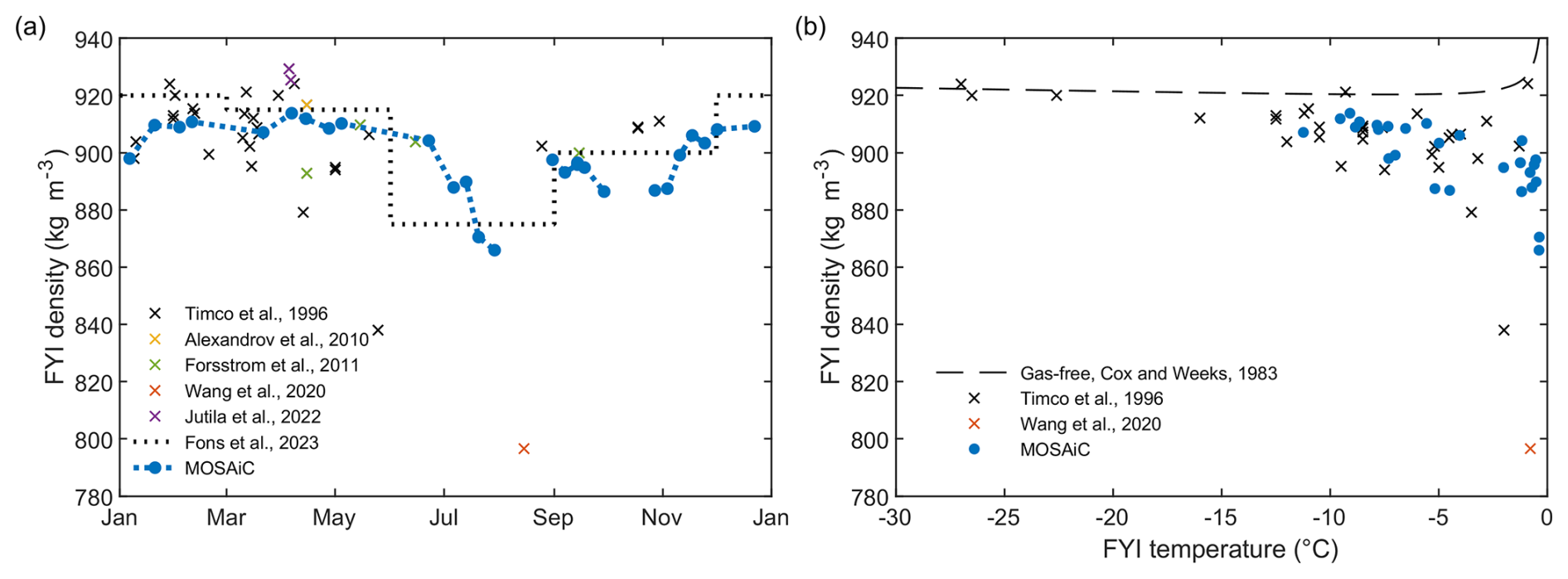
Figure 1 Panel (a) shows a historical overview of the seasonal evolution of FYI density including MOSAiC measurements presented in this study. Panel (b) shows the historical values of FYI density vs. its temperature. The dashed black line in (b) shows the density of gas-free ice with salinity of 2 calculated from Cox and Weeks (1983).

The bulk density of FYI (density of a composite material including pure ice, air, brine, and solid salts) varies seasonally (Fig. 1a), ranging from above 910 kg m⁻³ in winter (Alexandrov et al., 2010; Jutila et al., 2022) to below 900 kg m⁻³ in summer (Wang et al., 2020; Fons et al., 2023). Most observations show that bulk FYI density outside of the melt season is similar to pure ice density of 917 kg m⁻³, while SYI is significantly lighter (Timco and Frederking, 1996). Only a few studies have estimated sea ice density during the melt season, revealing a large range of values substantially lower than those from winter observations. Frantz et al. (2019) documented a notably strong decrease in sea ice density down to 600 kg m⁻³ as sea ice in Alaska became rotten and melted completely. FYI with higher temperatures displays lower density (Fig. 1b), including observations during summer (Wang et al., 2020) and autumn (Forsström et al., 2011).

Sea ice density depends on the volumetric fractions of ice, air, and liquid brine, usually estimated from measurements of bulk sea ice salinity, density, and temperature (Cox and Weeks, 1983). During the ice growth phase, the bulk brine fraction of columnar and congelation sea ice is usually below 5 % (Griewank and Notz, 2013) and the air volume fraction below the waterline is usually less than 2 % (Nakawo, 1983; Crabeck et al., 2016). Outside of the melt season, the temporal and spatial variability of sea ice density is quite low due to the small variability of both the bulk air and brine fractions (Fig. 1). Warming drives significant thermodynamic changes that increase the brine volume and air volume fractions. Light et al. (2003) and Crabeck et al. (2019) observed the shrinking of gas inclusions upon cooling and expanding during warming, suggesting that seasonal changes in temperature exert a strong control on the air volume fraction. While an increase in brine volume fraction tends to increase bulk ice density, an increase in air volume significantly lowers bulk ice density. Given that changes in the air fraction have a greater impact on sea ice density than changes in brine or ice volume due to the 10 times larger density difference between air and pure ice compared to that between pure ice and brine, it is questionable to neglect the impact of air volume fraction on bulk ice density.

In this study, we present observations of the temporal evolution of sea ice density, with a focus on its rapid changes during the melt season. We demonstrate how summer changes in sea ice impact the accuracy of ice thickness retrieval from freeboard measurements. We validate our density measurements using freeboard and draft measurements from ice coring, along with co-located underwater sonar and airborne laser scanner surveys. We assess the representativeness of the summer freeboard evolution with airborne freeboard measurements and validate sea ice thickness evolution using ice mass balance buoy data. This comparison is made between the 1 km² Multidisciplinary drifting Observatory for the Study of the Arctic Climate (MOSAiC) Central Observatory ice floe and observations from a surrounding area of approximately 50 km². Additionally, we analyze how the sea ice density is controlled by its air volume and the corresponding temperature evolution. We present seasonal sea ice density measurements for different ice types and examine how the observed seasonality relates to atmospheric and oceanic environmental forcing.

2 Methods

The MOSAiC Central Observatory (CO1), settled on an approximately 3 km by 4 km ice floe, drifted across the central Arctic from 4 October 2019 for a period of 10 months (Nicolaus et al., 2022). It followed the Transpolar Drift until it reached the ice edge in Fram Strait and broke apart on 31 July 2020 (Fig. 2a), with an area of 0.9 km² remaining during summer (CO2, Fig. 2b). We use observations from 23 FYI and 18 SYI coring events to obtain the temporal evolution of the draft, freeboard, density, salinity, and temperature of the main unponded ice types at the FYI and SYI coring sites and several ridges (Fig. 2b). To validate and extrapolate coring measurements of ice draft and freeboard to a larger area, we use ice draft measurements from remotely operated underwater vehicle (ROV) multibeam sonar (Katlein et al., 2022) and freeboard measurements from an airborne laser scanner (ALS; Hutter et al., 2023b). To validate ice melt rates obtained from ice coring and multibeam sonar, we use observations from ice mass balance buoys installed at the CO1 and in the distributed network (DN), covering a 40 km radius around it (Lei et al., 2022; Salganik et al., 2023a).

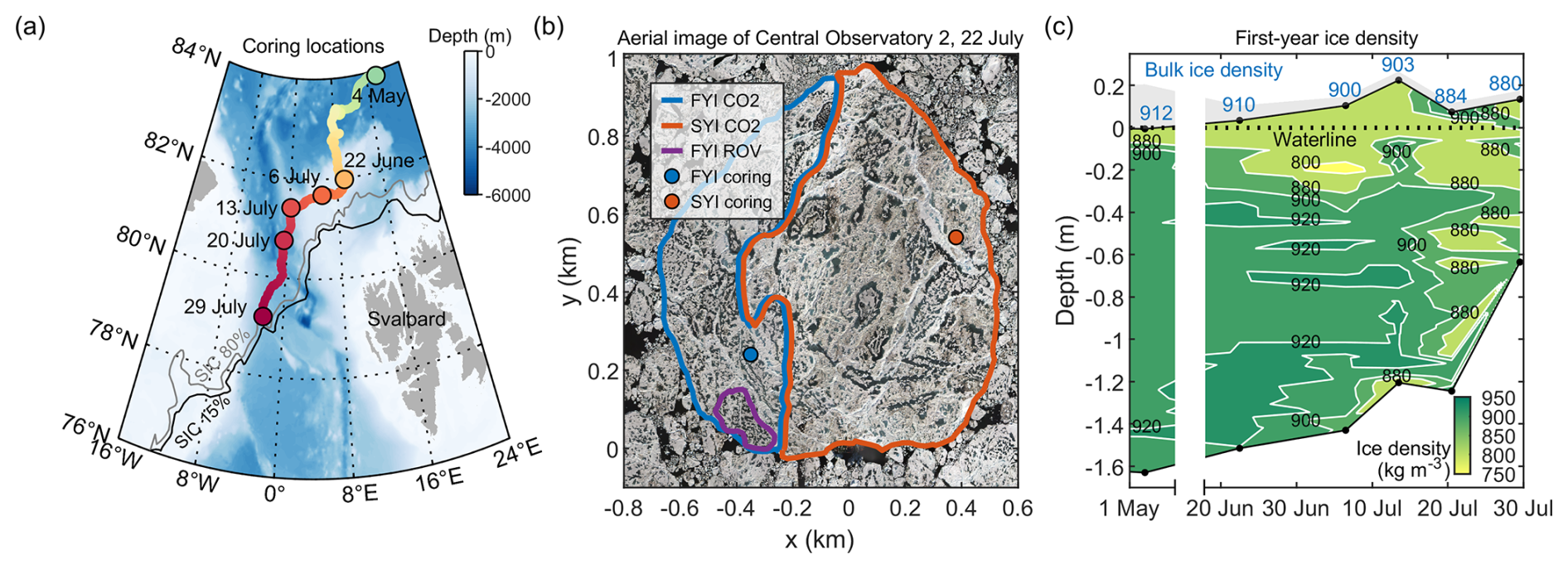
Figure 2 Panel (a) shows an overview map of the study area with the drift of the MOSAiC ice floe for coring observations from 4 May to 29 July 2020. Panel (b) shows the locations of first-year ice (FYI) and second-year ice (SYI), coring sites, and ROV sonar surveys on an optical aerial image of the Central Observatory (CO2) from 22 July from Neckel et al. (2023). Panel (c) shows the contour plot of FYI density evolution from hydrostatic weighing with bulk density values for each coring event shown in blue, and gray shaded areas represent snow or surface scattering layer thickness. Displayed bathymetric data in (a) are from ETOPO2 (National Geophysical Data Center, 2006) using Pawlowicz (2023), and displayed ice edges in (a) are derived from the AMSR-2 sea ice concentration (SIC) product for thresholds of 15 % and 80 % on 29 July 2020 (Spreen et al., 2008). Solid black lines in (c) with black circles representing each coring event show ice surface and bottom interfaces relative to the waterline shown as a dashed black line. The time axis in (c) is not continuous.

2.1 Ice coring and ice mass balance buoys

Sea ice freeboard and thickness were directly measured by drilling through the ice at two coring sites (Fig. 2b), while sea ice surface and bottom melt were estimated with ice mass balance buoys (IMBs). Ice cores were extracted using a Kovacs Mark II and III Core Barrels; 72.5 mm diameter core barrels were used for density measurement and 90 mm diameter core barrels for temperature and salinity cores. To minimize spatial variability, FYI and SYI cores were collected within a 130 m distance. However, each core is slightly different and cannot be interpreted as a continuous in situ time series. One coring event each week yielded a total of 20–30 cores for FYI and SYI sites. After extraction, the freeboard and draft of the cores were measured directly on-site using Kovacs ice thickness gauge. One temperature profile with a 0.05 m vertical resolution was made per coring event immediately after the core was extracted. The density and salinity cores were packed in plastic bags and transported into the ship's freezer room at a temperature of −15 °C. Density measurements (Fig. 2c) were performed by sectioning one core per event into 0.04–0.06 m long pieces in a cold lab, followed by hydrostatic density measurements by weighing ice sections in air and kerosene (Pustogvar and Kulyakhtin, 2016). The practical salinity of each melted piece was measured with a YSI 30 conductivity meter.

The relative brine volume of each section was calculated following Cox and Weeks (1983) and Leppäranta and Manninen (1988) for in situ conditions using the ice temperature profile measured in the field. The relative air volume $v_{\mathrm{a}}^{\prime }$ at laboratory temperature T=T_lab was estimated as follows:

$$\begin{array}{}\text{(1)}& v_{\mathrm{a}}^{\prime }=\mathrm{1}-{\displaystyle \frac{\mathit{\rho }}{{\mathit{\rho }}_i}}+\mathit{\rho }{S}_i{\displaystyle \frac{F_{\mathrm{2}}\left(T\right)}{F_{\mathrm{1}}\left(T\right)}},\end{array}$$

where ρ is the sea ice density measured in the lab, ρ_i is the pure ice density, S_i is the measured sea ice salinity, and F₁ and F₂ are temperature-dependent coefficients calculated from Cox and Weeks (1983) and Leppäranta and Manninen (1988) for temperatures below and above −2 °C, respectively. Sea ice density ρ_si at in situ temperature T=T_i and disconnected air and brine pockets, further referred to as weighing density, was calculated as

$$\begin{array}{}\text{(2)}& {\mathit{\rho }}_{\mathrm{si}}=(\mathrm{1}-v_{\mathrm{a}}^{\prime }){\displaystyle \frac{{\mathit{\rho }}_i{F}_{\mathrm{1}}\left(T\right)}{F_{\mathrm{1}}\left(T\right)-{\mathit{\rho }}_i{S}_i{F}_{\mathrm{2}}\left(T\right)}}.\end{array}$$

The estimate of sea ice density from the measurements of ice freeboard and draft, snow thickness, and density is referred to here as the effective sea ice density. Assuming the ice is at hydrostatic equilibrium, the effective sea ice density can be estimated as

$$\begin{array}{}\text{(3)}& {\mathit{\rho }}_{\mathrm{si},\mathrm{eff}}={\displaystyle \frac{{\mathit{\rho }}_{\mathrm{sw}}{d}_i-{\mathit{\rho }}_{\mathrm{sn}}{h}_{\mathrm{sn}}}{h_i}},\end{array}$$

where h_i is the ice thickness, d_i is the ice draft, ρ_sw is the seawater density, h_sn is the snow/SSL thickness, and ρ_sn is the snow/SSL density. Here we used density measurements of snow and the surface scattering layer (SSL, deteriorated granular melting ice similar to large-grained melting snow) from Macfarlane et al. (2023b). Due to its granular structure, snow and SSL could not be distinguished during coring and transect measurements, and here we refer to both snow and SSL as snow (Macfarlane et al., 2023a). The density estimate from snow and ice freeboard and thickness measurements at each coring site is further referred to as coring density.

To study the spatial variability of sea ice melt, we used nondestructive temperature measurements from IMBs. These buoys, which operate with internal heating cycles, allow for precise identification of snow–ice and ice–water interfaces (Jackson et al., 2013). We employed two types of IMBs: 13 SIMBA buoys (Lei et al., 2022) and 5 DTC buoys (Salganik et al., 2023a). The study included direct measurements of sea ice melt from 18 and 7 IMBs, operating from 22 June to 15 and 28 July, respectively. Two IMBs were located within CO2, 10 in CO1, and the remaining at DN. Approximately 20 % of IMBs were installed in level FYI, while the other 80 % were located in level or deformed SYI. We also used IMBs to estimate under-ice water temperature and density outside of coring sites, where water temperature was measured directly.

2.2 Airborne laser scanner (ALS) and remotely operated underwater vehicle (ROV)

The helicopter-based airborne laser scanner (ALS) Riegl VQ-580 provides values of snow, snow-free ice (SSL), or melt pond freeboard with kilometer-scale areal coverage, a spatial resolution of 0.5 m, and an elevation accuracy of 0.025 m. Freeboard conversion from ALS elevation measurements was performed using an automated open-water detection scheme using differences in open-water reflectance (Hutter et al., 2023b). The standard error of modal freeboard estimates was 0.02 m based on ALS surveys from Hutter et al. (2023a). In this study, we used nine ALS surveys conducted on 21 March, 8 and 23 April, 10 May, 30 June, and 4, 7, 17, and 22 July 2020. These surveys covered 0.5–0.9 km² of CO2, with total scanned areas of 75, 49, 57, 58, 49, 5.4, 3.2, 4.7, and 43 km², respectively. To calculate ice freeboard from snow/SSL freeboard measured by ALS, we used snow/SSL thickness measurements from near-daily Magnaprobe transects at the CO2 (Webster et al., 2022). In spring, we applied the average transect snow thickness for CO2 to the full ALS scan scale, while for the level FYI site at CO2 we used the average transect snow thickness for level ice as derived by Itkin et al. (2023). Gaps in freeboard for the ALS data over ponds at the nadir of the helicopter survey (3 %–8 % of the scanned area) were filled by bilinearly interpolating freeboard at the pond edges.

Multibeam sonar (DT101, Imagenex, Canada) mounted on a remotely operated vehicle (ROV; M500, Ocean Modules, Sweden; after Katlein et al., 2017, and Anhaus et al., 2025) provides measurements of ice draft over an area approximately 350 m by 200 m (Fig. 2b), with 0.05 m vertical accuracy and 0.5 m horizontal resolution (Coppolaro, 2018). Surveys were conducted in a grid pattern with a line spacing of 20–25 m. Seven surveys at a depth of 20 m with nearly 100 % overlap were performed during the melt season (from 24 June to 28 July 2020), near the floe edge of the CO2 ice floe. False bottoms were detected using the temporal evolution of ice draft measured by sonar before and after the melt pond drainage, and in this study, we focus on the part of sonar surveys not affected by false bottoms (Salganik et al., 2023b). To account for the time difference of 1–3 d between ALS and ROV surveys in summer, we linearly interpolated ALS freeboard and ROV draft measurements to align them with a daily interval and compute the bulk sea ice density. The pre-melt estimates of density are calculated using freeboard measurements from four ALS scans in March–May and ice draft measured by ROV on 30 June assuming ice growth and melt between March–June from IMB level ice measurements. The sea ice density estimate from ALS, ROV, and transect measurements is further referred to as density at the FYI ROV site.

Kilometer-scale ALS surveys include areas with different ice types and notably ridges. Ridges occupy a substantial fraction of the ice pack (Melling and Riedel, 1996), affecting the mass and hydrostatic balance of sea ice (Salganik et al., 2023d). Based on measured snow freeboard, we divided ALS observations into two classes: non-ridged sea ice, referred to here as level ice, and ridged sea ice in order to compare ALS freeboard evolution of different ice types and to remove freeboard biases caused by the spatial variability of the ridge areal fraction. For summer observations, characterized by thin snow (Webster et al., 2022), we identified ridges using a 0.35 m threshold above the modal snow freeboard. The snow freeboard threshold corresponds to the sail width of a ridge, investigated by both ALS and ROV sonar on 30 June. The estimated average ratio of the keel and sail width was 2.7 from the co-located ridge surface and bottom topography, which aligns with the ratio of 3 reported by Strub-Klein and Sudom (2012). For spring observations with substantially thicker snow, we used a 0.5 m threshold above the modal snow freeboard similar to Ricker et al. (2023).

2.3 Melt ponds

The accumulation of surface meltwater in ponds impacts the effective sea ice density by adding extra weight from meltwater, provided the ponds are raised above sea level, which replaces the lighter sea ice, snow, or SSL. To estimate sea ice density while accounting for the impact of surface melt ponds on the hydrostatic balance of an ice floe, we use the near-daily measurements of melt pond areal fraction and depth from Webster et al. (2022) for CO2, as well as melt pond depth reconstructed from aerial photographs using photogrammetry from Fuchs et al. (2024) for the ROV site (Fig. 2b).

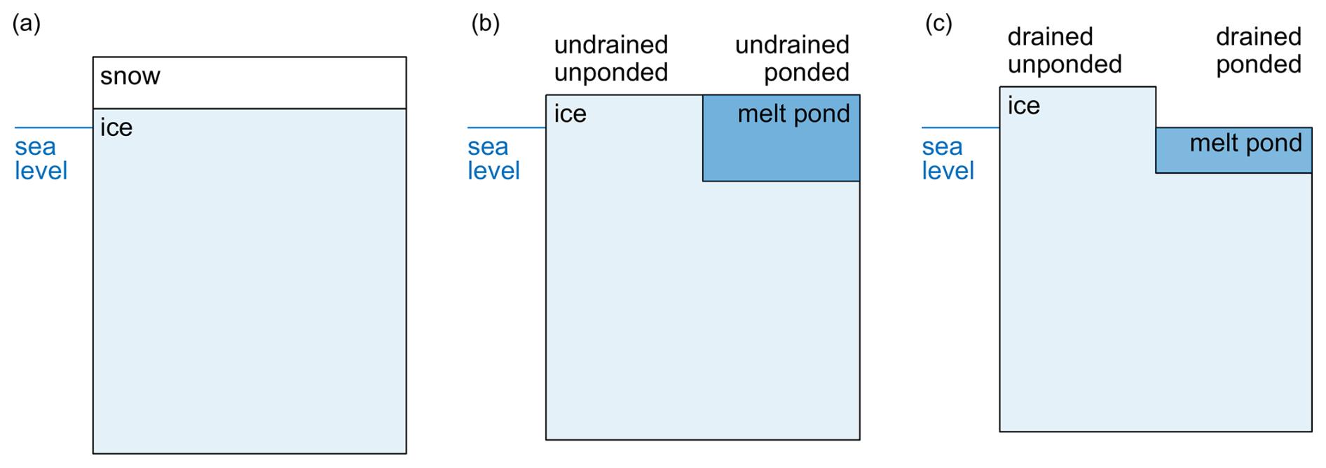
Figure 3 Illustration of different freeboard and draft for pre-melt sea ice (a) and for sea ice with undrained (b) and drained (c) melt ponds.

We distinguish the surface topography of ice covered with melt ponds (ponded) and not covered with melt ponds (unponded) surrounding ponded ice following Webster et al. (2022) (Fig. 3). Ponded areas are initially undrained but may become drained when meltwater is partially or completely transferred from the melt pond to the ocean (Eicken et al., 2002). Unponded ice located next to drained melt ponds is referred to here as drained unponded ice. The uplift of sea ice following melt pond drainage can be described analytically following the scheme and parameterization from Landy et al. (2014). For drained melt ponds, there is a noticeable difference between the freeboard of ponded ice and the unponded ice around it. This difference depends on whether melt ponds are deep enough to retain some meltwater after drainage, which happens when the initial melt pond depth h_mp exceeds the freeboard of drained unponded ice surrounding the drained melt pond. For shallow melt ponds with zero melt pond depth after drainage, the ice freeboard of drained unponded ice fb_d,up can be found as

$$\begin{array}{}\text{(4)}& {\mathrm{fb}}_{\mathrm{d},\mathrm{up}}=h_i-{\displaystyle \frac{{\mathit{\rho }}_{\mathrm{si}}(h_i-a_{\mathrm{mp}}{h}_{\mathrm{mp}})+{\mathit{\rho }}_{\mathrm{sn}}{h}_{\mathrm{sn}}(\mathrm{1}-a_{\mathrm{mp}})}{{\mathit{\rho }}_{\mathrm{sw}}}},\end{array}$$

where h_i is the ice thickness and a_mp is the melt pond fraction. The freeboard of ponded areas after pond drainage is fb${}_{\mathrm{d},\mathrm{up}}-h_{\mathrm{mp}}$. For melt ponds deeper than the freeboard of unponded ice, the unponded ice freeboard equals

$$\begin{array}{}\text{(5)}& {\mathrm{fb}}_{\mathrm{d},\mathrm{up},\mathrm{deep}}={\displaystyle \frac{({\mathit{\rho }}_{\mathrm{sw}}-{\mathit{\rho }}_{\mathrm{si}})(h_i-a_{\mathrm{mp}}{h}_{\mathrm{mp}})-{\mathit{\rho }}_{\mathrm{sn}}{h}_{\mathrm{sn}}(\mathrm{1}-a_{\mathrm{mp}})}{{\mathit{\rho }}_{\mathrm{sw}}(\mathrm{1}-a_{\mathrm{mp}})}}.\end{array}$$

The ice freeboard of sea ice before melt pond drainage can be found as

$$\begin{array}{}\text{(6)}& {\mathrm{fb}}_{\mathrm{ud}}={\displaystyle \frac{({\mathit{\rho }}_{\mathrm{sw}}-{\mathit{\rho }}_{\mathrm{si}})(h_i-a_{\mathrm{mp}}{h}_{\mathrm{mp}})-{\mathit{\rho }}_{\mathrm{sn}}{h}_{\mathrm{sn}}(\mathrm{1}-a_{\mathrm{mp}})}{{\mathit{\rho }}_{\mathrm{sw}}}}.\end{array}$$

For undrained ponds, we assume that the ice freeboard is the same for both ponded and unponded areas. For ponded and drained ice with deep ponds, we assume a zero melt pond freeboard. For drained melt ponds, the effective sea ice density depends on whether the freeboard of ponded areas is considered. For each scenario (drained or undrained) and ice type (ponded or unponded), the effective sea ice density can be found from the corresponding freeboard value using Eq. (3). If the ice freeboard of both ponded and unponded areas fb_i is measured, for the meltwater density ρ_mw, the effective sea ice density can be found as

$$\begin{array}{}\text{(7)}& {\mathit{\rho }}_{\mathrm{si},\mathrm{eff}}={\displaystyle \frac{{\mathit{\rho }}_{\mathrm{sw}}{d}_i-{\mathit{\rho }}_{\mathrm{sn}}{h}_{\mathrm{sn}}(\mathrm{1}-a_{\mathrm{mp}})-{\mathit{\rho }}_{\mathrm{mw}}{h}_{\mathrm{mp}}{a}_{\mathrm{mp}}}{(d_i+{\mathrm{fb}}_i)(\mathrm{1}-a_{\mathrm{mp}})+(d_i+{\mathrm{fb}}_i-h_{\mathrm{mp}})a_{\mathrm{mp}}}}.\end{array}$$

This equation allows estimating the effective sea ice density based on the measurements of the unponded and ponded freeboard from ALS, ice draft from sonar, snow/SSL thickness from a transect, melt pond depth and area from photogrammetry, and snow/SSL density from snow pits. The snow/SSL freeboard is the sum of ice freeboard fb_i and snow thickness h_sn.

3 Results

We present observations of the temporal evolution of sea ice density, air and brine volume, thickness, and freeboard during the melt season through spring and summer. We validate density measurements from weighing using various measurements of ice freeboard and draft, including ice coring and comparison to co-located ALS and ROV sonar surveys. We further upscale freeboard measurements using ALS surveys, and we validate sea ice melt measurements using data from IMBs. Finally, we present the seasonal evolution of sea ice physical parameters for undeformed first- and second-year ice and ridges.

3.1 Temporal evolution of sea ice density during the melt season

A strong decrease in bulk FYI density was recorded by all observing platforms during the summer melt (Table 1). Measurements of sea ice density from weighing at the FYI coring site gradually decreased from 910 kg m⁻³ on 22 June to 880 kg m⁻³ on 29 July, with a pre-melt density of 912±2 kg m⁻³ during 15 coring events from 14 November to 4 May (Fig. 4b). The effective density estimates from the FYI coring measurements showed a similar decrease in summer, from 909 kg m⁻³ on 22 June to 860 kg m⁻³ on 29 July, with a pre-melt density of 918±33 kg m⁻³. A combination of ALS freeboard and ROV sonar draft measurements produces an effective density at the FYI ROV site with a pre-melt value of 926±4 kg m⁻³ in March–May, which decreased to 912 kg m⁻³ on 30 June and further to 884 kg m⁻³ on 22 July. The effective sea ice density, derived from Eq. (7) to account for melt ponds at the FYI ROV site, was 6–8 kg m⁻³ lower than estimates without melt pond correction (Fig. 4b).

Table 1 Bulk physical properties of level first-year ice at the coring and ROV sites.

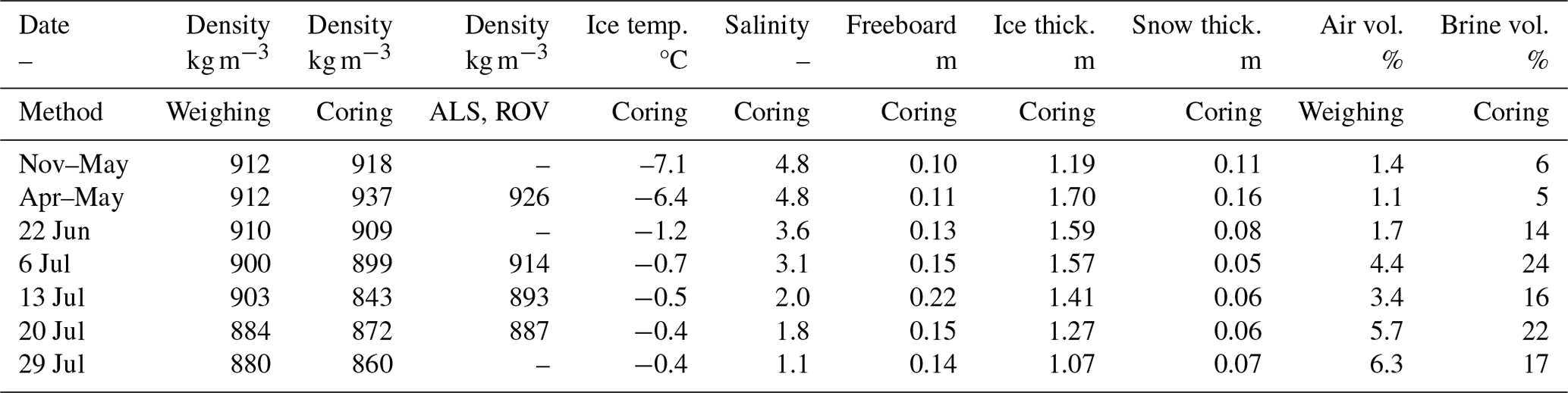
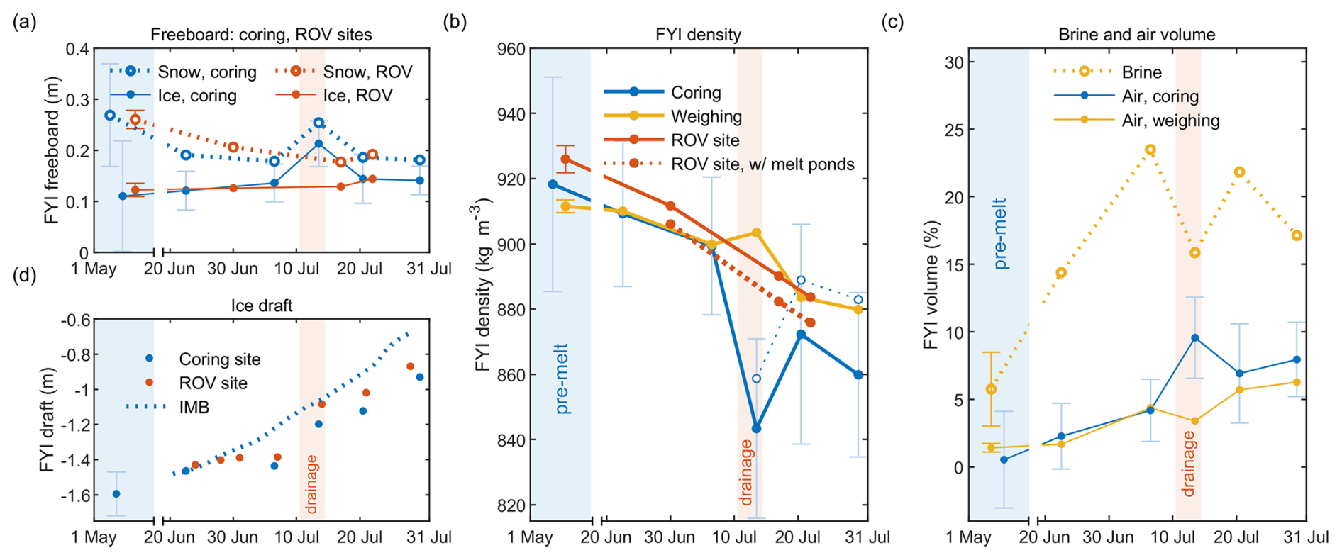
Figure 4 Summer evolution of first-year ice (FYI), snow, and ice freeboard (a), bulk density (b), brine and air volume (c), and draft (d) at the FYI coring and FYI ROV sites shown in Fig. 2b. In (a) FYI the snow/SSL and ice freeboard were measured manually at the coring site and using an airborne laser scanner (ALS) at the ROV site. In (b) FYI density was estimated from coring freeboard and draft measurements at the coring site (blue lines), from weighing (yellow lines), and from ALS freeboard and ROV draft measurements at ROV site (red lines). In (c) FYI brine volume was estimated using salinity and temperature measurements at the coring site, and FYI air volume was estimated using manual freeboard and draft measurements at the coring site and from weighing. The dotted blue line in (b) represents sea ice density estimate corrected for coring measurements performed in unponded areas as described in Sect. 4.6. Error bars represent 1 standard deviation of weekly measurements in summer or of all pre-melt weekly measurements for each type of measurement. The time axis is not continuous.

3.2 Temporal evolution of air and brine volume during the melt season

The air volume fraction of FYI derived from weighing density measurements and effective density from coring measurements using Eq. (1) showed a strong increase from May to July (Fig. 4c). The FYI air fraction, obtained using weighing, increased from 1.4±0.3 % in December–June (15 cores) to 3.4 %–6.3 % in July (four cores). While weighing measurements showed a slight density decrease during the melt pond drainage event, the air volume fraction from coring density estimates showed an increase. The estimate of FYI brine volume, obtained using measurements of ice salinity and temperature, increased from 6±1 % in December–June (15 cores) to 19±4 % in July (four cores). FYI air volume had, on average, a 2.5 times larger effect on bulk FYI density than brine volume.

3.3 Temporal evolution of snow and ice thickness and freeboard during the melt season

The melt season was characterized by a rapid decrease in ice thickness, starting in late June. All observing platforms (i.e., FYI coring, ROV sonar, and IMBs) showed an ice draft of around 1.4 m in late June, which fell below 1 m by the end of July (Fig. 5e). Level ice thickness decreased by 0.51 m from 22 June to 29 July at the FYI coring site, by 0.56 m at the FYI ROV sonar site, and by 0.67±0.20 m for IMBs in the DN in a 40 km radius around the main ice floe (Fig. 5d). Thicker ice types, such as SYI and ridges, experienced more rapid melt than FYI, with total ice melt measured as 0.93 and 1.77 m, respectively, by ROV sonar between 24 June and 28 July (Fig. 5d). While all observing platforms agreed on the magnitude and timing of the melt, there were minor differences in the recorded values.

Figure 5 Panels (a), (b), and (c) show the freeboard evolution of various ice types for small-scale (FYI coring and ROV sites), floe-scale (CO2), and large-scale (ALS full survey) measurements, respectively. Panel (d) shows accumulated ice melt measured by coring, ice mass balance buoys (IMBs), and ROV sonar for ridge, first-year ice (FYI), and second-year ice (SYI) after 24 June. Panel (e) shows ice draft measured by FYI coring, measured by ROV sonar, and estimated from IMB measurements of snow and ice thickness, assuming hydrostatic equilibrium. The level in (b) and (c) refers to ice outside of ridged areas following the classification described in Sect. 2.2.

Despite the decrease in ice thickness during late June and July, the ice freeboard increased at both the FYI coring and FYI ROV sites (Fig. 5a) and across the entire CO2 floe (Fig. 5b). At the FYI coring site, the ice freeboard was initially 0.13±0.04 m on 22 June and increased to 0.14–0.15 m during 6–29 July. Similarly, ALS measurements at the FYI ROV site between 30 June and 22 July showed a 0.02 m ice freeboard increase and a 0.01 m snow/SSL freeboard decrease (Fig. 6a–d). At the FYI coring site, the freeboard increased rapidly to 0.22±0.05 m during a melt pond drainage event on 13 July (Fig. 5a).

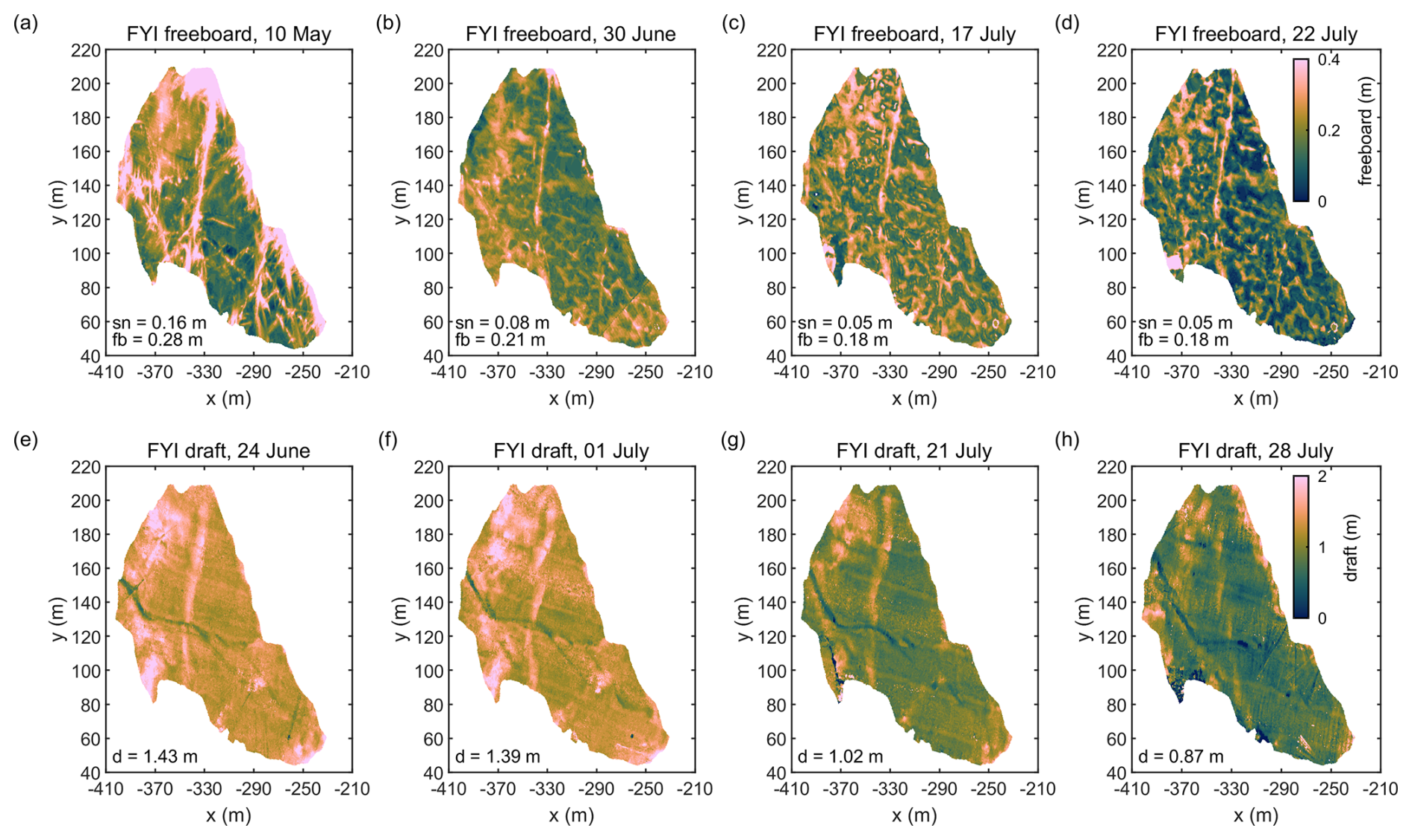
Figure 6 Snow or surface scattering layer freeboard from an airborne laser scanner (a–d) and ice draft from underwater sonar surveys (e–h) for selected dates covering the first-year ice area of ROV sonar surveys marked in purple in Fig. 2b. The average values of snow thickness (sn), freeboard (fb), and ice draft (d) for each survey are shown in black.

For the CO2 ice floe from June to July, the areal fractions of level FYI, level SYI, and ridge sails were 31 %, 57 %, and 12 %, respectively. From ALS surveys on 30 June and 22 July, the CO2 ice freeboard increased by 0.036 m for level FYI and stayed unchanged for level SYI. For the full ALS coverage, the freeboard of level ice increased by 0.014 m (Fig. 5c). Sea ice freeboard evolution from May to July was consistent across different scales from FYI coring and ROV sonar sites (0.014 km²) to ALS CO2 (0.9 km²) and ALS full coverage (40–50 km²), with overall minor changes in ice freeboard during July (Fig. 5a–c).

3.4 Seasonal evolution of sea ice physical parameters

In previous sections, we presented the summer evolution of FYI air volume, density, freeboard, and thickness. Here we present the annual evolution of the key physical parameters controlling FYI and SYI hydrostatic balance (snow and ice thickness, freeboard) and density (air and brine volume, ice temperature, and salinity).

3.4.1 Seasonal evolution of sea ice air volume and density

We observed a strong seasonality in the air volume of FYI and a weaker seasonality for SYI. At the beginning of the growing season (end of October), the mean air volume fraction of FYI was 3.9 %. It quickly decreased to below 2 % by early December as the ice cover cooled and became mostly impermeable, with the mean brine volume fraction dropping below the permeability threshold defined as 5 % following Golden et al. (1998). During the same period, the bulk FYI density increased from 893±10 to 908±8 kg m⁻³ (Fig. 7g).

Throughout the winter, the ice column remained mostly impermeable, except for the warm bottom layer, and the mean air volume stayed below 2 % (Fig. 7f, h). The bulk FYI density remained stable around 912±2 kg m⁻³. At the end of May, the ice column became isothermal and fully permeable, with a brine volume fraction largely above the 5 % threshold (Fig. 7f). As the ice warmed and the brine volume fraction increased, the mean air volume fraction tripled in the ice column, reaching a mean value of 6.3 %. Simultaneously, FYI density dropped below 880 kg m⁻³.

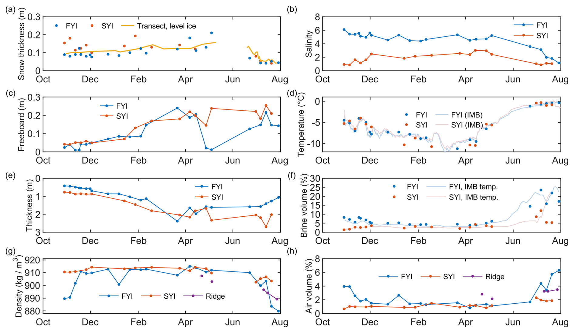
Figure 7 Annual evolution of snow/SSL thickness (a), bulk sea ice salinity (b), freeboard (c), temperature (d), thickness (e), brine volume (f), density (g), and air volume (h) for level first-year ice (FYI), level second-year ice (SYI), and ridges from the coring observations during MOSAiC in 2019–2020.

SYI air volume was stable during the freezing period and doubled from 1.0±0.2 % in the cold season (October to May) to 2.0±0.2 % in the summer in July (Fig. 7h). Consequently, the bulk SYI density decreased from 912±2 kg m⁻³ in October–May to 905±2 kg m⁻³ in June–July. In addition, four different ridges were sampled from 22 April to 27 July, exhibiting a similar decreasing density trend (Fig. 7g).

3.4.2 Similarities between seasonal evolution of first- and second-year ice

The seasonal evolution of SYI air fraction, density, and ice freeboard was similar to FYI, with nearly identical changes in ice freeboard based on observations of different scales (Fig. 7c). The maximum ice thickness of FYI and SYI, as measured by IMBs, was 1.75 and 1.94 m, respectively (Fig. 5e). This relatively small difference in thickness is because SYI at CO1 was formed in December 2018 and had a modal thickness of only 0.3–0.5 m by October 2019 (Krumpen et al., 2020; Itkin et al., 2023). This indicates that over 60 %–70 % of the pre-melt SYI thickness was formed during 2019–2020, sharing physical properties similar to the FYI. We focused on FYI physical properties due to the less extensive sampling of SYI. However, both FYI and SYI at CO2 experienced similar ice freeboard increases of 0.02 and 0.01 m, respectively (Fig. 5b), suggesting similar changes in their bulk densities and air volume fractions.

4 Discussion

4.1 Importance of sea ice density evolution for ice thickness estimation from its freeboard

The results of the full seasonal evolution of snow and ice thickness and freeboard, as well as bulk sea ice density, confirmed previous findings (e.g., Alexandrov et al., 2010) that during the growth season, changes in the ice freeboard are primarily caused by increasing ice thickness (Fig. 7c, e). While a decrease in freeboard during ice melt is expected, detailed observations during the early melt season revealed an increase or plateau in sea ice freeboard despite significant ice melt. Since most of the snow layer melted before early July, this freeboard increase is attributed to a reduction in bulk ice density, which enhances sea ice buoyancy. This was confirmed by ice freeboard measurements at the FYI and SYI coring sites, along with a combination of ALS measurements of snow freeboard and transect measurements of snow and SSL thickness for both level FYI and SYI within CO2.

4.2 Comparison with radar altimetry estimates of sea ice thickness

Sea ice thickness estimates from ice freeboard measurements using the CryoSat-2 radar altimeter (Landy and Dawson, 2022) showed a strong ice melt of 1.5 m between late May and June, followed by 0.6 m of melt in July (Fig. 8c). In contrast, IMBs measured only 0.06 m of accumulated ice melt in May–June and 0.64 m in July. Additionally, CryoSat-2 detected the onset of ice melt 1 month earlier than the actual data, coinciding with the onset of snowmelt. A similar mismatch in the timing of ice melt onset has been observed at the Beaufort Gyre mooring array (Dawson et al., 2022).

Figure 8 Vertical profiles of first-year ice (FYI) air volume (b) and density (d) during summer. Panel (d) shows accumulated ice melt from the CryoSat-2 ice thickness estimate from Landy and Dawson (2022), measured by IMB, and estimated from the IMB freeboard derived from IMB snow and ice thickness measurements assuming a constant pre-melt snow load and partial (70 %) snow penetration.

This discrepancy highlights known issues of the CryoSat-2 ice thickness data, as discussed in Landy et al. (2022). The first issue is related to the assumption that the meltwater load is immediately lost to the ocean as the snow mass decreases, as described in Eq. (3). This assumption is generally invalid during the early stages of melt, which could be seen in our ice freeboard observations in May–June (Fig. 4c). The second issue concerns the uncertain fraction of radar penetration through snow, which was assumed to be 90 % in Landy et al. (2022).

To test this potential explanation, we estimated snow and ice freeboard using IMB measurements of snow and ice thickness, applying Eq. (7) with the measured sea ice density. From these IMB freeboard estimates, we back-calculated ice thickness using a constant sea ice density of 917 kg m⁻³, as described in Landy et al. (2022). We considered two scenarios: one with constant pre-melt loading (snow and meltwater) and another with both constant snow loading and 70 % snow penetration. To align the ice type fraction between CryoSat-2 and IMB estimates, we assumed a pre-melt snow thickness of 0.3 m for all ice types, following transect observations. This value was consistent with MERRA-2 reanalysis data used in Landy et al. (2022).

The accumulated ice melt was 0.7 m observed by IMBs, 1.3 m from IMBs assuming a constant snow load, and 2.1 m from IMBs assuming constant snow load and 70 % snow penetration (0.08 m of pre-melt snow), as well as from CryoSat-2 freeboard measurements on 23 July. This suggests that approximately 40 % of the ice melt overestimation by CryoSat-2 can be attributed to the mistreatment of snow load, while the remaining 60 % is due to radar's inability to fully penetrate moist snow. Incorporating a physics-based parameterization of sea ice density could enhance the accuracy of altimetry measurements in order to capture sea ice melt instead of snowmelt. This is due to the observed snow freeboard decrease in July being equivalent to the CryoSat-2 ice thickness decrease (Fig. 5b). However, the depth of radar penetration into the snow remains a significant source of uncertainty in CryoSat-2 ice thickness estimates during snowmelt.

4.3 Comparison with previous measurements of sea ice density

The temperature dependence of our FYI density values closely matches historical observations for Arctic sea ice, showing a similar seasonal variability (Fig. 1b). The FYI density estimates for February–May by Alexandrov et al. (2010), based on in situ freeboard and draft measurements, indicated similar values of 917±36 kg m⁻³ (Fig. 1a). The FYI and SYI estimates from April by Jutila et al. (2022) were 925±18 and 899±17 kg m⁻³, respectively, showing larger values for FYI but smaller values for SYI (both 912±2 kg m⁻³ in our study). However, FYI and SYI thicknesses were similar in our study (Fig. 7b), whereas Jutila et al. (2024) observed SYI to be 3.2–4.5 m thick, 3–6 times thicker than adjacent FYI. Our observed seasonal variability of FYI density also closely matches the Antarctic FYI density estimates from Fons et al. (2023), derived from ship-based measurements from Worby et al. (2008), with summer and winter density values of 875 and 920 kg m⁻³, respectively (Table 1). We suggest that the parameterization from Fons et al. (2023) accurately describes the seasonality of Arctic FYI density and can be used in various applications including sea ice altimetry.

4.4 Comparison of methods for sea ice density estimation

Nearly all methods of measuring sea ice density have their disadvantages and limitations. Past studies have argued that ice coring leads to substantial brine loss during ice core extraction, particularly in permeable sea ice (Cottier et al., 1999; Notz, 2005), potentially leading to an artificial decrease in sea ice density. In our study, the sea ice density estimated from snow or ice freeboard and thickness measurements shows a similar trend to those computed from the weighing (Fig. 4b). During June–July, FYI density was equal to or slightly larger than the effective FYI density at coring and ROV sites, indicating no substantial impact of brine loss on weighing density measurements during the melt season. During the same period, the decrease in bulk FYI density was 30 kg m⁻³ from weighing, 26–49 kg m⁻³ based on coring, and 28–30 kg m⁻³ from co-located ALS and ROV observations (Fig. 4b).

Estimates of effective sea ice density from ice freeboard and thickness are not influenced by brine losses but typically exhibit much larger spatial variability of 10–30 kg m⁻³ than observations from weighing (Alexandrov et al., 2010; Hutchings et al., 2015; Jutila et al., 2022). Our coring measurements gave a standard deviation of 33 kg m⁻³, despite the freeboard being an average value from around 20–30 cores taken weekly, covering an area of around 10 m by 10 m (Fig. 4b). This is likely related to the large spatial variability of ice freeboard and draft (Fig. 7b) rather than true spatial variability of in situ sea ice density, as sea ice cannot bend to account for meter-scale deviations from its hydrostatic balance (Fuchs et al., 2024). We estimated the small-scale spatial distribution of the effective sea ice density using Eq. (3), smoothing the data from the ALS freeboard and ROV sonar draft over a 10 m window (as for coring). Similarly to coring, ALS observations revealed large meter-scale spatial variability in sea ice density, ranging from 15 to 32 kg m⁻³ (Fig. 9a, d).

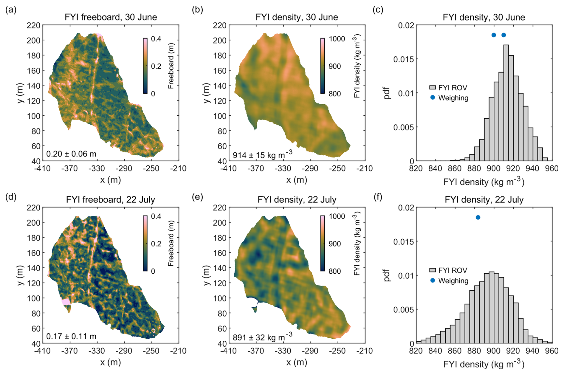
Figure 9 Contour plot of snow/SSL freeboard from an airborne laser scanner (a, d), contour plot of effective sea ice density (b, e), and histogram of effective sea ice density (c, f) for co-located draft measurements from sonar and freeboard from ALS for 30 June and 22 July at the FYI ROV site. The effective sea ice density was estimated using Eq. (3) from freeboard and draft values, smoothed using two-dimensional convolution with a 10 m wide window.

Winter observations (14 coring events) using the weighing showed a bulk FYI density standard deviation of only 2 kg m⁻³. Similarly low variability (5 kg m⁻³) when weighing nine FYI and seven SYI cores located 5 m from each other was observed during fall in Nansen Basin (Hornnes et al., 2025). These observations support the notion of meter-scale spatial variability in sea ice density of a few kg m⁻³, despite an order of magnitude larger variability in the effective sea ice density.

While our summer observations are characterized by a thin and homogeneous SSL (Webster et al., 2022), snow thickness in winter and spring shows large spatial variability. We found that in early May, snow thickness measurements from IMBs showed 0.16±0.02 m for level FYI (three buoys) and 0.23±0.07 m for level SYI (10 buoys). Snow thickness at coring sites in January–May averaged 0.13±0.04 m for eight FYI coring events and 0.14±0.03 m for four SYI coring events (Fig. 7a). Transect observations showed a large spatial variability of snow thickness above level ice of 0.16±0.12 m in May (Fig. 7a). These measurements illustrate the substantial spatial variability of snow thickness above level ice within CO1, obtained using various methods. Eq. (3) indicates that the uncertainty in sea ice density is 5–10 kg m⁻³ per 0.01 m of snow/SSL for a known snow freeboard and 1–3 kg m⁻³ per 0.01 m of snow/SSL for a known ice freeboard. The observed seasonal variability of FYI density, which ranges from around 30–60 kg m⁻³ (Fig. 4b), corresponds to snow/SSL thickness uncertainties of 0.04–0.08 m. These uncertainties are comparable to standard deviations of snow thickness measured by IMBs, coring, and transects. This limits the applicability of density estimates based on snow freeboard measurements to the larger areas where snow thickness was not directly measured.

We demonstrated that hydrostatic weighing is one of the most reliable and affordable methods for measuring sea ice density. Unlike other methods, it does not rely on the assumption that gravity and buoyancy forces acting on sea ice are in hydrostatic equilibrium at all scales. Our measurements of sea ice freeboard and draft indicate that this equilibrium is not satisfied for scales less than tens of meters, resulting in 1 order of magnitude greater spatial variability in sea ice density for methods based on this assumption compared to the direct density measurements from weighing. The effective density estimates from the measured ice freeboard and draft of cores, and by ALS, ROV and satellite observations, converge only after more than 100 measurements are taken, reflecting uncertainties in other terms of the hydrostatic balance rather than true ice density variability. Finally, weighing does not rely on measurements of snow thickness, which is characterized by a large spatial variability outside of the melt season.

4.5 Geochemistry of air volume evolution

The bulk density of sea ice is determined by the volume fractions of its constituent phases: ice, brine, and air. Among these, the air volume has the most significant impact on the bulk density. As illustrated in Figs. 4b and 7g–h, the observed decrease in bulk FYI density during the melt season corresponds to an increase in air volume fraction throughout the ice column (Fig. 8a). The air volume fraction in columnar ice (based on ice texture from Nicolaus et al., 2022) exceeded 4 %, reaching over 10 % in the sea ice surface layer above the waterline (Figs. 10a and 8). This increase is synchronized with the rise in the brine volume fraction as the ice warms, indicating a strong link between the air volume fraction and the thermodynamic state of sea ice (Fig. 7).

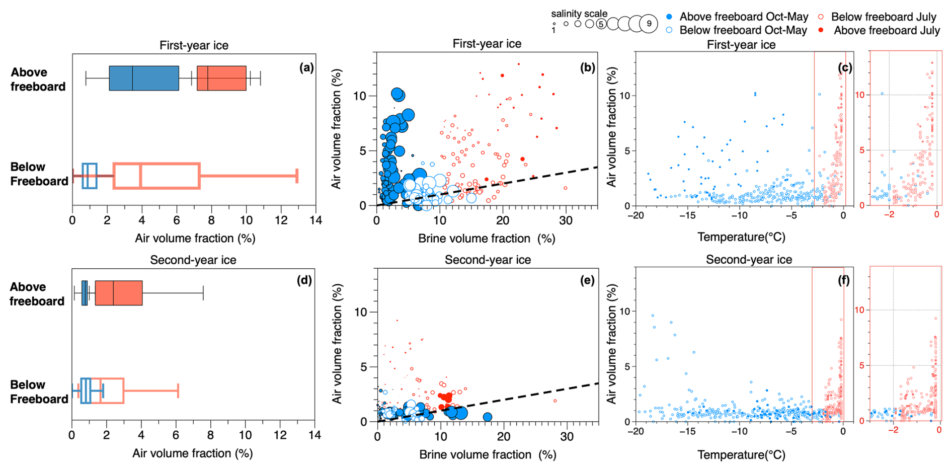
Figure 10 First-year ice (FYI) and second-year ice (SYI) air volume distribution (a, d) and the relationship between the air volume fraction and the brine volume fraction (b, e) and temperature (c, f). The dashed lines in (b) and (e) represent the volume of air formed due to a 10 % density difference between pure ice and brine during melt. The diameters of the circles in panels (b) and (e) are proportional to the ice sample salinity; smaller circles indicate lower salinity.

The ice above the waterline shows a systematic enrichment in the air volume fraction compared to the ice below the waterline (Fig. 10a, d) and for FYI appears to be decoupled from the thermodynamic state of sea ice, as the air volume is not correlated with the brine volume (Fig. 10b, c). This observation aligns with previous studies indicating that the air volume fraction in the upper ice layer is controlled by the formation of granular ice, snow ice, and superimposed ice. Frazil ice, which traps gas directly from the atmosphere during its formation, contains more gas than columnar ice (Tsurikov, 1979; Perovich and Gow, 1996; Cole et al., 2004; Zhou et al., 2013; Crabeck et al., 2016). Additionally, the random crystal alignment in frazil ice also reduces the efficiency of drainage processes that expel dissolved gases (Golden et al., 1998). As sea ice grows, the air volume fraction in the surface layers can increase due to the formation of snow ice and superimposed ice, which traps air bubbles inherited from the overlying porous snow cover (Cole et al., 2004; Crabeck et al., 2016). During the melt, as shown in Fig. 10a and b, the increase in air volume fraction is especially strong in the heavily desalinized ice layer (small solid red dots in Fig. 10b). This is because the flushing process leaves the previously brine-filled pockets in the ice layer above the waterline filled with air (Perovich and Gow, 1996).

In columnar ice below the freeboard, the air volume fraction shows a clear relationship with the brine volume fraction and temperature (Figs. 7 and 10b, c). Bubbles in columnar ice are often enclosed in brine inclusions (Light et al., 2003), so it is not surprising that their volumes are linked. Biogeochemical work on the aqueous–gaseous equilibrium in sea ice (Zhou et al., 2013; Moreau et al., 2014; Crabeck et al., 2019) suggests that the air volume depends on the potential phase change (from dissolved within brine to gaseous in air bubbles) that takes place in the brine medium. Observations indicate that gas inclusions shrink or disappear as brine cools (Light et al., 2003; Crabeck et al., 2019). Our observations reveal that during the coldest months (October to May), the air volume fraction decreased and stayed well below 2 % in FYI and SYI (Fig. 7c). As the brine inclusions shrink under cooling, the air bubbles contained within them also shrink under the compressive force of the freezing pressure present in a closed pocket (Crabeck et al., 2019). This freezing pressure results from the gradual volume expansion linked to the transformation of liquid water to solid ice, which compresses the trapped bubble and pushes gas into the solution.

As the ice warms, the brine and air volume fractions increase (Figs. 7, 10b, c). Previous studies have reported that columnar sea ice is typically depleted in air volume fraction, with gas volume less than 2 %, and that most air voids are found in the ice above the waterline – because below the freeboard, these voids would be filled with underlying seawater or meltwater (Tsurikov, 1979). However, our observations revealed a notable increase in air volume in columnar ice even below the freeboard as the ice warmed and became fully permeable (Fig. 8). Light et al. (2003) observed that warming brine inclusions lead to bubble enlargement, while Crabeck et al. (2019) reported the appearance of new bubbles in brine due to nucleation during warming. They related these bubbles' enlargement and nucleation to internal melt within the brine pockets. In our dataset, the increase in air volume fraction in columnar ice below the freeboard is particularly significant when the ice temperature is above −2 °C (Fig. 10c, d). Above −2 °C, the ice undergoes a heavy internal melt, characterized by the gradual transformation of ice into liquid brine. Tsurikov (1979) and Perovich and Gow (1996) suggested that the density difference of 10 % between ice and liquid during melting would result in the formation of voids filled with water vapor in sea ice. In SYI, the increase in air volume fraction closely follows this relationship (i.e., dotted line in Fig. 10e), and the increase is especially strong at the onset of pure ice melt close to 0 °C (Fig. 10f). For FYI, our observations show that the increase in air volume is significantly higher than the 10 % increase associated with ice melting (Fig. 10b). Crabeck et al. (2019) explained that voids formed by internal ice melt create a vacuum in the brine pockets, causing dissolved gases heavily concentrated in the liquid brine to nucleate into new bubbles and migrate to the gas phase, thus enlarging the bubble volume. This process is typical for FYI because it is more enriched in dissolved solutes (i.e., salt and dissolved gases) than SYI, which is depleted in salts and other solutes. Additionally, Fig. 10 (smallest red circles) shows that the most desalinized layers have the highest air volume fraction, suggesting that brine pockets could be possibly becoming filled with air even below the freeboard. Finally, it is important to note that while salts are efficiently rejected downward by brine drainage and flushing, gas tends to remain in the ice. Once gas nucleates into air bubbles, these bubbles are either trapped in the ice or move upward by buoyancy, leading to the accumulation of bubbles throughout the season.

The seasonal evolution of sea ice density is controlled by the temperature-dependent evolution of its air volume. As ice warms, the air volume within the ice column increases, reducing sea ice density (Fig. 7d, g). Conversely, warming also increases brine volume, which slightly counteracts this effect by increasing sea ice density. However, the impact of air on density is roughly 10 times greater than that of brine. A significant linear correlation (R²=0.4; pvalue $=\mathrm{1.5}\times {\mathrm{10}}^{-\mathrm{14}}$) between air volume v_a and ice temperature T for ice warmer than −1.3 °C ($v_{\mathrm{a}}=max(\mathrm{1.2},\mathrm{6.4}\cdot T+\mathrm{8.4})$; Fig. 10d) allows for a parameterization of sea ice density against its temperature together with the widely used dependence of brine volume on ice temperature and salinity using Eq. (2).

4.6 Accounting for melt pond drainage

The presence of melt ponds complicates ice thickness retrieval from satellite, airborne, or in situ freeboard measurements by introducing uncertainties related to the unknown volume of melt ponds (Landy et al., 2022). The formation of melt ponds adds hydraulic head (water height above sea level) and lowers the freeboard (Eicken et al., 2002). After melt pond drainage, ice below and surrounding the melt ponds experiences an uplift (Fuchs et al., 2024). In this section, we investigate the effect of melt ponds and their drainage on the freeboard of ponded and unponded ice. Our goal is to evaluate the biases in sea ice density estimates for measurements partially (like ALS) or fully (like coring) performed at unponded ice.

The presence of undrained melt ponds had a minor effect on ice freeboard. Equation (6) indicates that undrained melt ponds result in an increase in the effective sea ice density of 2–6 kg m⁻³ if melt ponds are not considered. Following melt pond drainage, Eqs. (4) and (5) suggest that the increase in the freeboard for unponded areas surrounding drained melt ponds was 0.03–0.04 m. The correction of the estimated 15–23 kg m⁻³ difference in effective sea ice density for all and only unponded ice areas allowed for better agreement between FYI density estimates from weighing and coring (Fig. 4b). We cannot fully account for the 0.07 m ice uplift observed at the FYI coring site, which could be attributed to substantial meter-scale spatial variability in the sea ice freeboard (Fig. 9a, d). On a larger scale, pond drainage likely caused a 0.03 m ice uplift for CO2 (Fig. 5b) and a 0.05 m uplift for the full ALS scan (Fig. 5c), aligning with our analytical estimates.

In this section, we evaluated the potential effect of both drained and undrained melt ponds on estimates of the effective sea ice density. Considering the presence of melt ponds helps reduce biases in freeboard measurements conducted partially or fully at sea ice without melt ponds. We also demonstrated that melt pond drainage causes an uplift of unponded ice, observable on different scales. The magnitude of this uplift can be described analytically, although small-scale freeboard observations from coring are subject to significant spatial variability, making measurements of such uplift less accurate.

4.7 Impact of ridges

In this section, we show that before the melt season, the investigated CO2 ice floe had a thicker snow thickness than the surrounding ice due to a significantly higher ridge fraction. The uneven spatial distribution of ridges questions the validity of upscaling snow thickness measurements to areas outside the sampling sites.

Ridges complicate ALS analysis by substantially increasing the freeboard due to thicker ice and snow in winter and through their enhanced melt in summer. To improve the intercomparison of freeboard evolution using different methods, we categorized all ALS freeboard measurements into level ice and ridge classes using a threshold derived from the co-located observations of a ridge freeboard and draft from ALS and sonar. During summer, we found that the CO2 had an areal fraction of ridge keels of 32±5 %, which was significantly larger than ridge keel fraction of 22±4 % for the full ALS scans. The main importance of ridges for ice thickness retrieval from snow freeboard measurements lies in their ability to increase surface roughness, which leads to the accumulation of substantially thicker snow above and around them (Itkin et al., 2023). This complicates the upscaling of ice thickness retrieval from snow freeboard, as snow thickness can vary significantly in areas with different ridge fractions. Therefore, the pre-melt estimates of ice thickness from ALS snow freeboard measurements outside of CO1 are uncertain, as snow thickness was only measured within CO1 and CO2 ice floes, which had unrepresentative ridge fractions.

Snow thickness can vary on a kilometer scale. ALS measurements in April–May showed 0.12–0.17 m larger snow freeboard values and a 1.5 times larger ridge areal fraction at CO2 compared to the surrounding area (Fig. 5b, c). Our estimate of the areal ridge fraction – 32 % for CO2 and 22 % for the full ALS scans – assuming 2 m level ice thickness from IMBs and a typical ridge thickness of 6 m (Strub-Klein and Sudom, 2012) would explain only a 0.03 m difference in the average snow freeboard between CO2 and the ALS full scans, with the remaining freeboard difference attributed to variations in snow thickness. For level ice, the ALS snow freeboard was 0.10–0.14 m larger for CO2, which is comparable to the absolute values of the observed level ice freeboard. The fraction of level FYI at CO2 was 31 %, while for full ALS coverage Kortum et al. (2024) estimated a level FYI fraction of 50 %. This suggests that CO2 had an unrepresentative small fraction of level FYI with typically thinner snow. This indicates significant uncertainties in sea ice density estimates using pre-melt snow freeboard measurements due to substantial spatial variability of snow thickness on different scales. The absence of large uncertainties related to snow/SSL thickness variability during the melt season supports the enhanced accuracy of effective ice density estimates during the snow-free period. For winter observations, this reveals the advantages of sea ice density estimates from hydrostatic weighing, not affected by snow thickness uncertainties.

Ridges not only affect snow thickness distribution but are also characterized by more complex thermodynamics than level ice, including larger melt rates (Salganik et al., 2023e). Meanwhile, although ridges were undersampled compared to level ice (with only four sampling events), the temporal evolution of the sea ice density of ridges was similar to FYI (Fig. 7g), as well as the freeboard evolution of both ridge and level ice during the melt season (Fig. 5b, c). Overall, the sea ice freeboard with and without ridges experienced a similar snow and ice freeboard evolution during the melt season, suggesting that ridges have a similar temporal density evolution to FYI.

5 Conclusions

In this study, we present weekly observations of first- and second-year ice density from hydrostatic weighing. During the melt season, the bulk density of first-year ice decreased from 910 to 880 kg m⁻³, while the bulk density of second-year ice showed a smaller decline from 912 to 905 kg m⁻³. The observed seasonal changes in sea ice density were primarily due to the rapid increase in air volume fraction during the melt season. For first-year ice, the bulk air volume fraction rose from 1 % to 6 %, and for second-year ice, it increased from 1 % to 2 %. Our seasonal dataset indicates that the previous assumption that columnar sea ice below the freeboard always has a depleted air volume fraction (i.e., less than 2 %) is no longer valid. The substantial increase in air volume fraction across the whole ice column during the melt season significantly affects sea ice buoyancy and its freeboard. The increase in air volume is strongly related to two factors: (1) internal melt, which creates voids, enlarges bubbles, and nucleates new bubbles, and (2) the replacement of liquid brine by air in drained inclusions.

The measurements of first-year ice density were validated using weekly ice freeboard and draft measurements from ice coring, as well as co-located snow freeboard measurements from an airborne laser scanner and ice draft measurements from underwater sonar. Both methods showed a comparable decreasing trend in first-year ice density, similar to the direct density measurements from hydrostatic weighing, with around a 30 kg m⁻³ decrease during June–July.

We demonstrated that hydrostatic weighing is one of the most reliable and affordable methods for measuring sea ice density, providing estimates with typically an order of magnitude lower uncertainty than those obtained from combined freeboard, draft, and thickness observations. Density estimates from measurements of snow or ice freeboard and ice draft are characterized by larger variability and are complicated by the presence of melt ponds in summer. Upscaling of these estimates during winter is complicated due to the large-scale spatial variability of snow thickness given the variability of ridge fraction.

The decrease in sea ice density during the melt season leads to non-decreasing values of its freeboard, which complicates estimates of sea ice melt from altimetry measurements. During June–July, we measured the total melt of level ice to be 0.6–0.7 m using ice coring, underwater sonar, and ice mass balance buoys. Despite the absence of snow above level ice in July, this ice loss was accompanied by an increase in the first-year ice freeboard of 0.02 m at the coring site and at the area of the co-located laser scanner and underwater sonar observations. For the whole 0.9 km² of the investigated ice floe, the level ice freeboard also increased by 0.03 m, while the freeboard of the surrounding 50–60 km² experienced an increase of 0.01 m in level ice areas. Our study underscores the necessity of accounting for seasonal changes in sea ice density, particularly the air volume fraction, for more accurate ice thickness retrievals. We showed that both our and historical observations of sea ice density reveal its strong dependence on sea ice temperature and salinity, with the range of summer density decrease potentially making around half of typical summer thickness loss not detectable from ice freeboard observations without accounting for the density evolution.