Greenland Ice Sheet surface roughness from Ku- and Ka-band radar altimetry surface echo strengths

Surface roughness is an important factor to consider when modelling mass changes at the Greenland Ice Sheet (GrIS) surface (i.e., surface mass balance, SMB). This is because it can have important implications for both sensible and latent heat fluxes between the atmosphere and the ice sheet and near-surface ventilation. While surface roughness can be quantified from ground-based, airborne, and spaceborne observations, satellite radar datasets provide the unique combination of long-term, repeat observations across the entire GrIS and insensitivity to illumination conditions and cloud cover. In this study, we investigate the reliability and interpretation of a new type of surface roughness estimate derived from the analysis of Ku- and Ka-band airborne and spaceborne radar altimetry surface echo powers by comparing them to contemporaneous laser altimetry measurements. Airborne data are those acquired during the 2017 and 2019 CryoVEx (CryoSat Validation Experiment) campaigns, while the satellite data (ESA CryoSat-2, CNES–ISRO SARAL, and NASA ICESat-2) are those acquired in November 2018. Our results show GrIS surface roughness is typically scale-dependent. A revised empirical mapping between quantified radar backscattering and surface roughness gives a better match to the coincident laser altimetry observations than an analytical model that assumes scale-independent roughness. Surface roughness derived from the radar surface echo powers is best interpreted not as the wavelength-scale RMS deviation representative of individual features but as the continued projection of scale-dependent roughness behaviour observed at baselines hundreds of metres long down to the radar wavelength. This implies that the relevance of these roughness estimates to current SMB modelling efforts is limited, as surface roughness is treated as a homogenous and scale-independent parameter.

1 Introduction

The satellite mass balance history of the Greenland Ice Sheet (GrIS) is a record of the balance between loss of snow, firn, and ice due to runoff, evaporation, sublimation, erosion, and calving and gain in the way of new precipitation (Otosaka et al., 2023; The IMBIE Team, 2020). It is the primary means of understanding Greenland's recent (e.g., 1990s–present) contribution to global sea-level rise and forms the basis for understanding ice sheet evolution in the future (Bamber et al., 2019; Edwards et al., 2021; Goelzer et al., 2020). There are three geodetic ice sheet mass balance observations: gravimetry, input–output, and altimetry (Otosaka et al., 2023). Gravimetric mass balance is based on monitoring changes in the gravity field across the ice sheet as mass lost through melting and/or discharge and the addition of new snow results in minute but detectable gravity fluctuations. The input–output method compares the quantity of material added to or lost from an ice sheet's surface (surface mass balance, SMB) to the amount of ice flowing through peripheral fluxgates. Finally, the altimetric mass balance approach is based on converting changes in ice sheet surface elevation (i.e., volume changes) to changes in mass. Critically, both the input–output and altimetry-based mass balance approaches require model-based estimates of the ice sheet SMB, which in the former defines the net mass change across the ice sheet surface and in the latter the non-mass-change component of the observed surface elevation change (i.e., due to firn compaction). Regardless, to quantify GrIS mass balance using either the input–output or altimetry approaches, insight into pan-ice-sheet SMB is paramount and is typically derived using numerical regional climate models (RCMs) (Alexander et al., 2019; Boberg et al., 2022; Bougamont et al., 2005; Ettema et al., 2009; Medley et al., 2022; Vernon et al., 2013).

Numerical estimates of GrIS SMB are based on coupled climate–subsurface models (van den Broeke et al., 2023). In this framework, a critical parameter to constrain is the roughness of the ice sheet surface as it modulates the energy balance between the atmosphere and the subsurface via sensible and latent heat fluxes along with near-surface ventilation (i.e., interstitial airflow through snow/firn) (Albert and Hawley, 2002; Amory et al., 2016; Braithwaite, 1995; Jakobs et al., 2019; Smeets and van den Broeke, 2008; van Tiggelen et al., 2021, 2023; van der Veen et al., 2009). Outside of affecting atmosphere–ice-sheet heat fluxes, surface roughness can also denote different morphogenetic areas of the ice sheet (Nolin et al., 2002; van der Veen et al., 2009), steer incipient supraglacial meltwater flow in the ablation zone (Cathles et al., 2011), and affect conventional laser and radar altimetry measurements of surface elevation change (Herzfeld et al., 2000; van der Veen et al., 2009; Yi et al., 2005).

Compared to other SMB-relevant parameters (e.g., temperature, precipitation, short- and longwave radiation, wind speed) surface roughness is unique because (1) it can be dependent on the scale over which it is quantified and (2) there are a variety of different metrics that have been used (Shepard et al., 2001). The most direct means of measuring GrIS surface roughness is with extremely local (i.e., metre-long) comb gauges and snow blades that produce centimetre-scale, one-dimensional replicas of the snow surface (Albert and Hawley, 2002; Jezek, 2007). Relevant statistical descriptions for surface roughness (e.g., peak-to-peak amplitude, roughness wavelengths) can then be quantified from these replicas. To extend the metre-scale local comb gauge/snow blade measurements, Herzfeld et al. (2000) developed a towed sensor capable of measuring surface elevations at fine spatial scales along profiles hundreds of metres in length. Fixed, ground-based laser-scanning measurements have also been used to characterize the two-dimensional distribution and growth of metre-scale snow bedforms (e.g., dunes, sastrugi) (Filhol and Sturm, 2015; Picard et al., 2019; Zuhr et al., 2021). While ground-based surface roughness measurements yield the finest spatial sampling, their large-scale applicability is limited as they are very time-consuming and subject to site accessibility (e.g., remoteness, weather) issues.

Furthermore, acquiring data on regional or pan-GrIS scales is extremely relevant for SMB flux calculations (van den Broeke et al., 2023). For this, remote sensing via airborne or satellite methods is the sole viable option. Photogrammetry and laser scanning from the air (i.e., drones, helicopters, planes) have each been used in regional surface roughness studies (Nolin et al., 2002; van Tiggelen et al., 2021; van der Veen et al., 2009). Still, similar to the in situ methods, accessibility throughout the year remains a challenge due to weather and illumination conditions. Satellite remote sensing can acquire data across the GrIS throughout the year, and, while optical and laser methods are still sensitive to illumination conditions (e.g., during the polar night) and cloud cover, respectively, radar techniques can operate year-round. GrIS surface roughness has been derived from various datasets collected by different satellites, including US Navy Geosat (Davis and Zwally, 1993), NASA ICESat (Yi et al., 2005), NASA ICESat-2 (van Tiggelen et al., 2021), and NASA Terra (Nolin et al., 2002). It is important to consider though that, while satellite remote sensing datasets can be used to characterize surface roughness over large areas, the horizontal sampling of the roughness is typically much coarser than ground-based methods. For example, the horizontal scales over which roughness is measured can vary from 1 m (van Tiggelen et al., 2021) to 10 km (Yi et al., 2005).

Recently, Scanlan et al. (2023a) presented a new approach for characterizing the monthly variability in surface roughness across the GrIS via the strength of radar altimetry surface echoes. Their approach is based on the Radar Statistical Reconnaissance (RSR) method (Grima et al., 2012, 2014b, 2022). As the name implies, RSR is a statistical approach that allows for the observed strength of radar echoes to be decomposed into their coherent and incoherent components and, when combined with a backscattering model, be used to derive the relative dielectric permittivity and RMS height of the surface. Initially developed to study Mars (Grima et al., 2012, 2022), the RSR method has also been applied to airborne VHF measurements of polar ice masses (Chan et al., 2023; Grima et al., 2014b, a, 2016, 2019; Rutishauser et al., 2016) and Ku-band radar altimetry measurements of the surface of Titan (Grima et al., 2017). Where Scanlan et al. (2023a) outline how the RSR method has been implemented for the analysis of Ku- and Ka-band radar altimetry measurements and perform a preliminary qualitative interpretation, this study focuses more intensely on the GrIS surface roughness results, with the specific goal of validating their derivation and interpretation. Only once the foundation of the surface roughness results has been solidified can their applicability with respect to SMB modelling be explored.

In this study, the reliability of the Ku- and Ka-band surface roughness estimates derived from the RSR analysis of radar altimetry surface echoes is assessed by comparing them to RMS deviations (Shepard et al., 2001) derived from laser altimetry measurements. This comparison is performed at both (1) locations of simultaneous airborne radar and laser altimetry collected as part of the 2017 and 2019 ESA CryoVEx (CryoSat Validation Experiment) campaigns in central Greenland and (2) a set of locations spanning the Greenland Ice Sheet using satellite (i.e., ESA CryoSat-2, CNES–ISRO SARAL, and NASA ICESat-2) datasets acquired in November 2018. The satellite comparison focuses on November 2018 as the RSR results are generated monthly (Scanlan et al., 2023a) and November 2018 is one of the first full months when ICESat-2 was completely operational following its launch 2 months earlier. We perform the comparison of radar and laser-altimetry-derived surface roughness for both the airborne and spaceborne cases for two reasons: first because the spatial resolution of the airborne datasets is much finer than the spaceborne datasets and second because the spatial coverage of the satellite data is much broader than that of the airborne datasets. Therefore, considering both yields a more complete understanding of the radar-altimetry-derived surface roughness results.

2 Datasets

2.1 CryoVEx altimetry

The series of CryoVEx (CryoSat Validation Experiment) campaigns operated by ESA focus on (1) validating satellite altimetry measurements over ice sheets and sea ice by way of repeated satellite ground track under flights and (2) supporting the design of future satellite altimetry missions (e.g., ESA CRISTAL, Sentinel-3 Next Generation Topography (S3NG-T)). To this end, through its history, the CryoVEx nadir-pointing airborne altimetry sensor package has included versions of different altimeters, but the most important for this study (Table 1) are ESA's Ku-band (13.5 GHz centre frequency, 0.1098 m range resolution) ASIRAS (Airborne SAR/Interferometric Radar Altimeter System) radar, the MetaSensing Ka-band (34.525 GHz centre frequency, 0.165 m vertical resolution) KAREN radar, and the Riegl LMS Q-240i-60 airborne laser scanner (ALS; 904 nm wavelength). All altimetry measurements are supported by precise aircraft positioning by combined GPS and INS (inertial navigation system) navigation solutions. In addition to the airborne platform, CryoVEx campaigns also include a substantial ground component tasked with installing corner reflectors on the surface and taking in situ measurements (e.g., density) in the shallow subsurface along the aircraft and satellite ground track.

Table 1 Summary of the airborne and satellite radar and laser altimetry datasets used to derive surface roughness as part of this study.

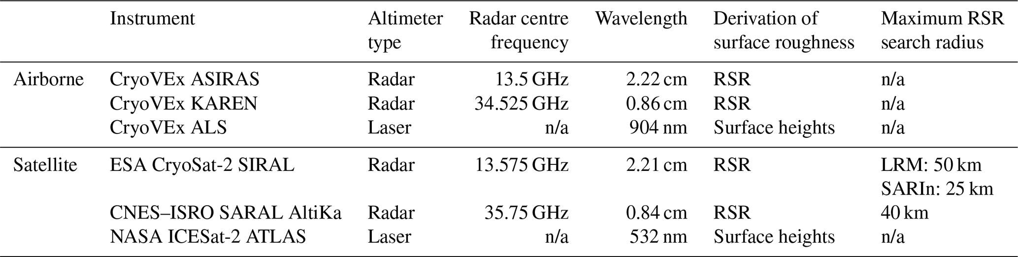
This study uses March and April 2017 (Skourup et al., 2019) and April 2019 (Skourup et al., 2021) CryoVEx data (ESA, 2022a, b) collected along the EGIG (Expéditions Glaciologiques Internationales au Groenland) line in central Greenland. Specifically, it focuses on ASIRAS, KAREN, and ALS measurements surrounding positions of the in situ measurements performed at the T5, T9, T12, T19, T30, and T41 locations in 2017 as well as T9, T12, T21, and T35 locations in 2019. All CryoVEx datasets are available, having already undergone thorough data processing (Skourup et al., 2019, 2021). Both the ASIRAS and KAREN data have been subject to post-acquisition SAR (synthetic aperture radar) processing to minimize the size of their respective footprints in the along-track (3 and 5 m, respectively) and across-track (10 and 12 m, respectively) directions. The ALS data have been calibrated, had outliers removed, and been organized into 200–300 m wide swaths following the aircraft ground track. Individual ALS ground height measurements are spaced at 1 m by 1 m intervals and have a vertical accuracy of ∼10 cm (Skourup et al., 2019, 2021).

2.2 Satellite altimetry

For decades, satellite radar and laser altimetry have been the method of choice for acquiring the ice sheet surface elevation change (SEC) measurements that feed long-term mass balance monitoring efforts (Abdalati et al., 2010; Markus et al., 2017; Otosaka et al., 2023; Schröder et al., 2019; Schutz et al., 2005; The International Altimetry Team, 2021). Of particular interest in this study (Table 1) are the Ku-band radar altimetry datasets from the SIRAL instrument (13.575 GHz centre frequency, 320 MHz bandwidth) on board the ESA CryoSat-2 spacecraft (Phalippou et al., 2001; Rey et al., 2001; Wingham et al., 2006) as well as the Ka-band measurements from the AltiKa instrument (35.75 GHz centre frequency, 500 MHz bandwidth) on board the CNES–ISRO SARAL spacecraft (Steunou et al., 2015; Verron et al., 2015). Laser altimetry measurements come from the ATLAS instrument (532 nm wavelength) on board the NASA ICESat-2 spacecraft (Abdalati et al., 2010; Markus et al., 2017).

Leveraging the results of Scanlan et al. (2023a), because CryoSat-2 operates in two different acquisition modes over Greenland, this study makes use of both Low-Resolution Mode (LRM) Level 1B (L1B) and SAR Interferometric (SARIn) Full-Bit Rate (FBR) CryoSat-2 Baseline-D data products. The LRM data products cover the GrIS interior, where CryoSat-2 waveforms are stacked from an individual 1.97 kHz pulse repetition frequency (PRF) to a constant data rate of 20 Hz. Across the GrIS margins, the CryoSat-2 SARIn data products contain reflected waveforms from 18.181 kHz PRF, 64-pulse bursts (burst repetition frequency of 21 Hz) acquired by both of CryoSat-2's receive antennas. The FBR data are preferred to higher-level SARIn data products (e.g., Level 1) as they have not yet been subject to any SAR focusing. The SARAL Sensor Geophysical Data Record (SGDR) data products are similar to CryoSat-2 LRM products in that initially 3.8 kHz PRF waveforms are averaged along-track in 25 ms (40 Hz) intervals. Finally, this study makes use of release 005 ATL06 ICESat-2 data products providing geolocated surface heights across the GrIS in 20 m increments. The quality summary variable included with each of the six beams in the ATL06 data products is used to reject lower-certainty surface height measurements.

3 Methods

3.1 Quantification of surface roughness from laser altimetry

As alluded to previously, quantifying surface roughness is not straightforward as it can be scale-dependent or scale-independent and multiple metrics have been put forward in the literature. Shepard et al. (2001) provide a thorough overview of various surface roughness metrics and how they can relate to one another. With the horizontal scale dependence of surface roughness a distinct possibility, this study adopts the strategy of Steinbrügge et al. (2020) and quantifies surface roughness by way of the RMS deviation.

Figure 1 presents a simplified overview of how to calculate the RMS deviation at various baselines from a set of measured surface elevations along a profile following Shepard et al. (2001). First, a constant background plane is removed from the measured surface elevations, yielding a profile of surface deviations (z(x_i) in Fig. 1a). Then the differences in height deviation are calculated for the n possible combinations of points along the profile that are spaced some defined horizontal distance (i.e., baseline) apart (e.g., Δx₁, Δx₂, and Δx₃ in Fig. 1). The RMS deviation for that specific baseline is then the RMS of all those height deviation differences following

$$\begin{array}{}\text{(1)}& v\left(\mathrm{\Delta }x\right)={\left\{{\displaystyle \frac{\mathrm{1}}{n}}{\sum }_{i=\mathrm{1}}^n\left[z\right(x_i)-z(x_i+\mathrm{\Delta }x){]}^{\mathrm{2}}\right\}}^{\mathrm{1}/\mathrm{2}}.\end{array}$$

Finally, the RMS deviation profile (Fig. 1b) presents how the RMS deviations vary as a function of the range of horizontal baselines considered (i.e., the horizontal scale dependency in surface roughness). While Fig. 1 presents the derivation of the RMS profile from a one-dimensional profile of surface elevations, the procedure can also be expanded to two-dimensional surface elevation datasets. In such an application, it is possible to derive both isotropic (i.e., baselines in all directions considered equally) and anisotropic (i.e., baselines restricted to only certain azimuth/cardinal directions) RMS deviation profiles. When presented in log–log space, it is common for the RMS deviation profiles (Fig. 1b) to exhibit a piecewise linear behaviour (Steinbrügge et al., 2020).

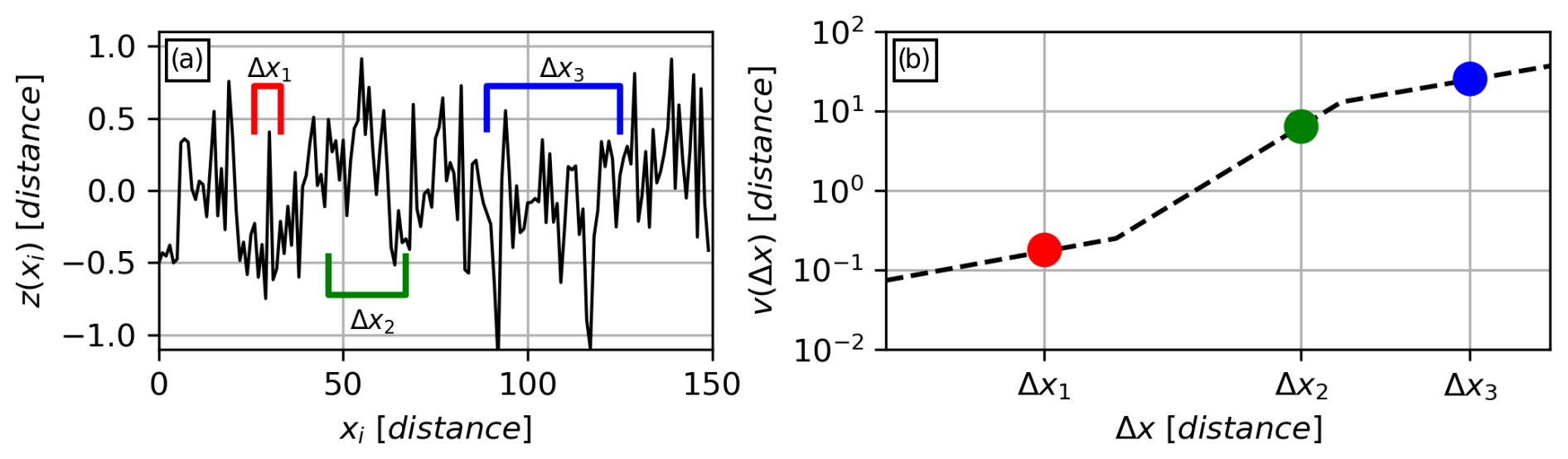
Figure 1 Simplified diagram demonstrating how to derive an RMS deviation (v(Δx)) profile that quantifies surface roughness as a function of horizontal baseline (Δx) for an artificial roughness dataset. The profile comprises the RMS of height deviations (i.e., elevations minus a background plane; z(x_i)) considering all combinations of points with a similar horizontal baseline. The RMS deviation profile (b) can be derived from profile data (i.e., as demonstrated here) as well as two-dimensional surface elevation datasets.

3.2 Radar statistical reconnaissance (RSR) implementation and calibration

As RSR is based on the statistical distribution of measured surface echo powers, the first step in implementation is to extract those surface echo powers from the measured waveforms. The same surface detection and extraction approach is applied to the CryoVEx (ASIRAS and KAREN) and satellite (CryoSat-2 and SARAL) datasets and follows Scanlan et al. (2023a). The leading edge is defined as the point of maximum integrated rate of change in the waveform amplitude when derived over different proportions of the receive window. For the airborne data, individual rates of change in the receive waveform amplitude are calculated over 2 % and 4 % of the receive window length, while for the satellite data, amplitude derivatives over 3 %, 6 %, and 9 % of the waveform receive windows are used. The extracted surface echo power is then the maximum power observed within 5 % of the range window following the re-tracked leading edge position. One feature relevant to the analysis of the airborne ASIRAS data is that the amplitudes provided in the CryoVEx data products have been normalized. Representative waveform amplitudes (A_rep) are generated from the normalized amplitudes (A_norm) following

$$\begin{array}{}\text{(2)}& A_{\text{rep}}=A_{\text{norm}}\times {\mathrm{10}}^{-\mathrm{9}}\times {\text{FAC}}_A\times {\mathrm{2}}^{{\text{FAC}}_B},\end{array}$$

where FAC_A and FAC_B are the linear scale factor A and power-of-2 scale factor variables reported in the ASIRAS data products. Once extracted, ASIRAS and KAREN surface power amplitudes are omitted from further analysis if the measured roll is greater than 1.5°. This threshold is determined empirically and used to limit the potential effects a rolling aircraft and off-nadir instrument pointing have on the strength of the surface echoes. For the satellite data, CryoSat-2 SARIn echo powers are removed if there is a marked CAL4 flag, while for SARAL, the altimetric range (>1000 km), a trailing edge variation flag, and a large average waveform off-nadir angle (>0.10 degrees squared) are all used to remove possibly erroneous surface echo powers. Finally, the satellite surface echo powers are also corrected for the nadir surface slope (Scanlan et al., 2023a) using the 500 m ArcticDEM (Porter et al., 2018), while the more local CryoVEx data are not.

Fundamentally, how the RSR method is implemented is the same for all the radar altimetry datasets. The set of radar surface echo amplitudes closest to some defined location is used to construct a histogram, and the statistical descriptors of the homodyned K-distribution fit (i.e., metrics quantifying the mean and spread) define the coherent (P_c) and incoherent (P_n) powers (Grima et al., 2014b). For the CryoVEx case, the locations are defined as the positions of in situ density measurements along the EGIG line (Skourup et al., 2019, 2021). The choice to focus exclusively on the immediate area surrounding in situ measurements allows for the rapid check of the reliability of the RSR approach when applied to CryoVEx data by way of reproducing in situ density estimates. For both ASIRAS and KAREN, RSR histograms are constructed from the 1000 closest surface echo powers to each in situ position (measured in EPSG:3413). For the satellite datasets, the CryoSat-2 LRM and SARAL results are taken directly from Scanlan et al. (2023a) (i.e., 5 km × 5 km grid, 1000 surface echo powers closest to each grid node). For the CryoSat-2 SARIn data, the same five-by-five grid is used, but instead of 1000 surface echo powers, the 12 000 closest samples are used to overcome the apparent statistical dependence of adjacent CryoSat-2 SARIn surface echo powers noted in Scanlan et al. (2023a).

Two metrics are used to quality control the RSR results: first the distance to the furthest surface echo power measurement considered and second the correlation coefficient between the observed surface echo power histogram and the statistical fit. The former is irrelevant for the CryoVEx data as we mandate using the closest 1000 data points surrounding the in situ locations regardless of how far they may be. For the satellite results, search radii of 50, 25, and 40 km are used for the CryoSat-2 LRM, CryoSat-2 SARIn, and SARAL results, respectively (Table 1). The CryoSat-2 LRM and SARAL maximum search radii are the same as those used in Scanlan et al. (2023a), while the CryoSat-2 SARIn radius is extended as more data points are being considered. A minimum correlation coefficient of 0.96 is required for all RSR results (Grima et al., 2012, 2014a, b; Scanlan et al., 2023a). This threshold is used to select only locations where the envelope of observed surface echo powers can be well described by the homodyned K distribution, which includes implicit assumptions for how radar energy is scattered from the surface (Grima et al., 2014b). As such, locations that do not meet this correlation coefficient threshold are not necessarily of poorer quality but require a different interpretation of the observed echo powers. This study however focuses solely on locations described well by the homodyned K-distribution statistics.

Once coherent (P_c) and incoherent (P_n) powers are determined, deriving surface roughness requires adopting a representative backscattering model. The simplest implementation of the RSR technique (Grima et al., 2012, 2014a, b; Scanlan et al., 2023a) assumes incoherent backscattering from the surface follows the small perturbation model (SPM) (Ulaby et al., 1982). In this case, surface RMS height can be derived following

$$\begin{array}{}\text{(3)}& {\mathit{\sigma }}_{\mathrm{h}}={\displaystyle \frac{\mathit{\lambda }{e}^{P_{\mathrm{n}}/\mathrm{2}{P}_{\mathrm{c}}}}{\mathrm{4}\mathit{\pi }\sqrt{P_{\mathrm{c}}/P_{\mathrm{n}}}}},\end{array}$$

where λ is the signal wavelength [m]. In contrast to RMS deviation (Eq. 1), RMS height is simply the standard deviation of the surface heights (after removing the mean) with no consideration of horizontal scale (Shepard et al., 2001). The validity bounds of the SPM are kσ_h<0.3 and kl<3 where k is the radar wavenumber [m⁻¹] and l is the surface roughness correlation length [m]. The analytical relationship for deriving RMS height from the RSR results in Eq. (3) is based on the assumption that the surface roughness correlation length (i.e., the length scale over which the roughness occurs) is large relative to the radar footprint and can be neglected (Grima et al., 2012, 2014b). A subtle feature of this approach for both the CryoSat-2 LRM and SARAL results is that the along-track stacking inherent in the L1B and SGDR datasets (see Sect. 2.2) makes the RSR results more sensitive to the surface roughness correlation length in the along-track direction (Grima et al., 2014b). Stacking preferentially enhances reflections from tilted roughness elements fore and aft of the stacking midpoint, increasing their contribution to the total received power and accentuating the along-track correlation length. However, any impact due to CryoSat-2 LRM and SARAL stacking is assumed to be minimal.

In contrast to when deriving surface dielectric permittivities from the RSR results, the absolute calibration of the RSR coherent powers is not directly required to produce a roughness estimate (Grima et al., 2012, 2014b, a; Scanlan et al., 2023a). However, as an additional check on the overall applicability of the RSR approach, CryoVEx RSR results have been calibrated using the contemporaneous in situ measurements. The CryoVEx P_c and associated calibration density values vary between 2017 (189.5 dB and 0.438 g cm⁻³ for ASIRAS; 324.6 dB and 0.353 g cm⁻³ for KAREN) and 2019 (183.7 dB and 0.57 g cm⁻³ for ASIRAS; 317.25 dB and 0.5 g cm⁻³ for KAREN) and are based on the same assumed Ku- and Ka-band density depth sensitivity as used in Scanlan et al. (2023a). Once calibrated, the coherent powers returned from the RSR analysis are related to the Fresnel reflection coefficient for an air–snow/firn interface ($r=(\mathrm{1}-\sqrt{{\mathit{\epsilon }}_{\mathrm{r}}})/(\mathrm{1}+\sqrt{{\mathit{\epsilon }}_{\mathrm{r}}})$, where ε_r is the relative dielectric permittivity of the snow/firn) following

$$\begin{array}{}\text{(4)}& P_{\text{c,cal}}=r^{\mathrm{2}}{e}^{-(\mathrm{2}k{\mathit{\sigma }}_{\mathrm{h}}{)}^{\mathrm{2}}}.\end{array}$$

Multiple empirical functions exist for then converting relative dielectric permittivity to snow density (Ambach and Denoth, 1980; Kovacs et al., 1995; Pomerleau et al., 2020; Tiuri et al., 1984).

4 Comparisons of radar and laser altimetry surface roughness estimates

4.1 Airborne CryoVEx datasets

The results of the CryoVEx RSR analysis are presented in Fig. 2. All EGIG sites visited in 2017 and 2019 have been analysed. However, it should be noted that in the case of T35 (grey circle in Fig. 2a), which was visited in 2019, the ASIRAS and KAREN RSR results both failed the quality control assessment and no data from this location are presented. The comparison of the measured in situ average densities (top 2 m for KAREN and top 4 m for ASIRAS; Scanlan et al., 2023a) with those derived from the RSR analysis demonstrates that we can reasonably recover the in situ densities from the remote sensing measurements after calibration (Fig. 2b). Comparisons of the 2017 and 2019 surface roughness results from the ASIRAS, KAREN, and ALS altimetry datasets are presented in Fig. 2c and d, respectively. It is assumed that the ASIRAS (triangles) and KAREN (squares) RMS heights derived from Eq. (3) are equivalent to the ALS RMS deviations at a horizontal baseline equal to the respective radar wavelength (Table 1).

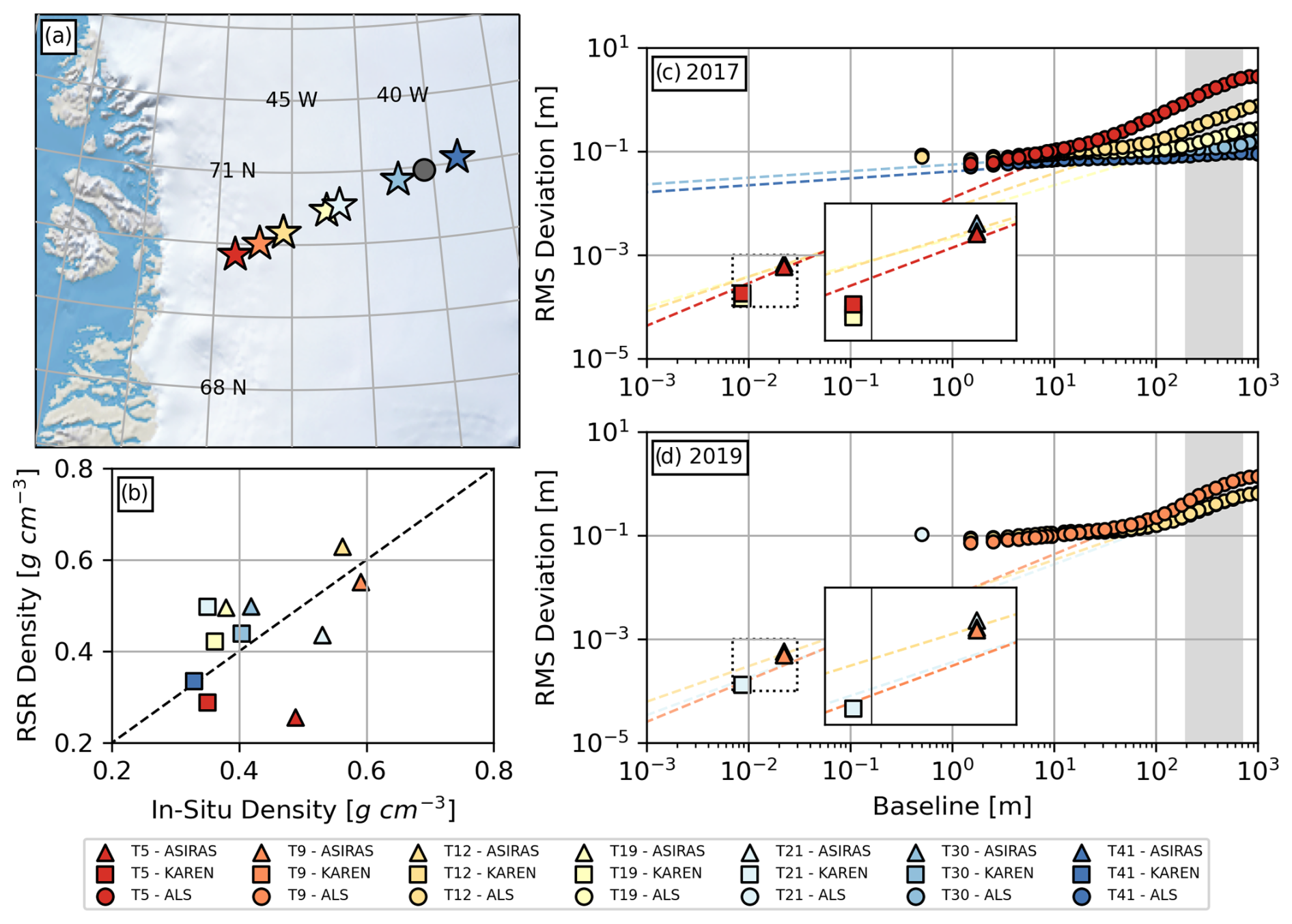
Figure 2 Results from the analysis of 2017 and 2019 airborne CryoVEx data. The locations of the in situ measurements along the EGIG line are presented in panel (a). Panel (b) presents the agreement (R of 0.45) between the RSR-derived densities from ASIRAS (triangles) and KAREN (square) surface echo powers with those measured in situ. The comparisons of RMS heights from the radar altimetry (assumed to be equivalent to the RMS deviation at the wavelength baseline) and the ALS (circles) RMS deviations as a function of baseline are presented in panels (c) (CryoVEx 2017) and (d) (CryoVEx 2019). Inserts in panels (c) and (d) present zoomed-in views of the RSR results. The RSR-based roughness estimates align well with the projection of the piecewise linear portion of the ALS RMS deviations profiles between 200–700 m (i.e., the grey region) to the radar wavelength baseline.

The ALS-derived RMS deviation profiles presented in Fig. 2c and d exhibit surface roughness behaviour that does not immediately align with the RSR results. At short (< 100 m) baselines, the ALS RMS deviation profiles are relatively flat and therefore not strongly dependent on the horizontal scale over which roughness is measured. The situation changes though at long baselines (>100 m) where there is a stronger scale dependency as progressively larger RMS deviations are measured for longer baselines. The fundamental pattern is then one of two piecewise linear components: a flatter, less scale-dependent behaviour at small baselines and more scale dependency at longer baselines. It is then clear that the continuation of the piecewise linear trends in RMS deviation from baselines less than 50 m to the radar wavelengths would overestimate the RSR results by roughly 2 orders of magnitude. However, projecting the linear, scale-dependent behaviour at longer baselines (e.g., between 200 and 700 m) yields the dashed lines in Fig. 2c and d, which closely intersect with the initial values derived from ASIRAS and KAREN. This suggests that surface roughness derived through the RSR analysis of CryoVEx radar altimetry surface echo powers is not a scale-independent RMS height but the wavelength-scale projection of surface roughness behaviour observed at long baselines. It should be noted, however, that this interpretation assumes that there are no further inflexion points at baselines smaller than those that can be accessed via the ALS data.

Amongst the ALS results, the 2017 T30 and T41 RMS deviation profiles (Fig. 2c) are unique in that they do not exhibit the increased scale-dependent roughness behaviour at longer baselines. Instead, their RMS deviation profiles are flatter and monotonic (i.e., not piecewise linear). The reason for this change in surface roughness behaviour is due to the ALS data surrounding T30 and T41 preferentially covering extremely smooth local areas of the GrIS. Figure 3 presents the local surface elevations (Fig. 3a and b) along with the height deviations (elevations minus the constant location-specific background plane; Fig. 3c and d) surrounding the T30 and T41 ALS datasets. Elevations are taken from the 10 m ArcticDEM mosaic (Porter et al., 2018), and the background plane is defined using all 10 m ArcticDEM data within 20 km of the CryoVEx in situ measurement location. Dataset-specific (i.e., ALS, ICESat-2, ArcticDEM) background planes are used to ensure all calculated height deviations have a mean of zero (Shepard et al., 2001) and accurately reflect the local conditions over which the data are acquired (needed when comparing to the RSR results). It is clear that the topographic variability is very small at T30 and essentially non-existent at T41. It is then not surprising that the corresponding RMS deviation profiles (Fig. 2c) do not exhibit the increase in RMS deviation at large horizontal baselines that is observed at the other CryoVEx locations. To further emphasize the smoothness of the GrIS near T30 and T41, Fig. 4 compares the ALS RMS deviation profiles with those derived from all ICESat-2 surface elevations within 25 and 35 km of T30 and T41, respectively. We must use ICESat-2 data that are further away from the T30 and T41 sites because these locations are between ICESat-2 orbital ground tracks. When considering surface topography over a broader regional area (i.e., ICESat-2), the stronger scale dependency in surface roughness is once again observed. Less scale dependency exists in the ALS RMS deviation profiles between 100 m and 1 km because T30 and T41 are situated in a locally very smooth portion of the GrIS (Fig. 3).

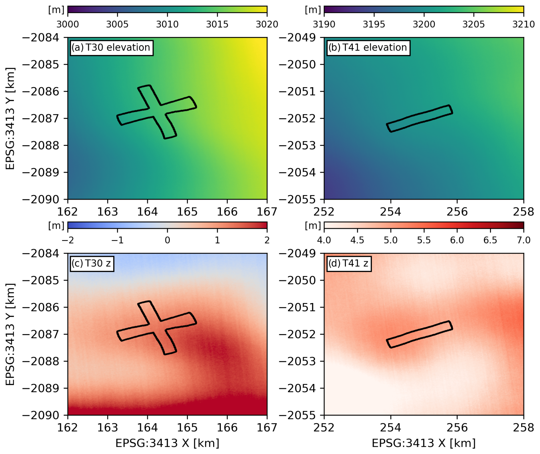
Figure 3 Surface elevations (a, b) and height deviations (c, d) surrounding the T30 (a, c) and T41 (b, d) CryoVEx locations. The ALS data considered in deriving the corresponding RMS deviation profiles in Fig. 2c come from within the black polygons. It is clear that T30 and T41 are sited in locally smooth regions of the GrIS. Note the change in colour bar and associated limits between (c) and (d).

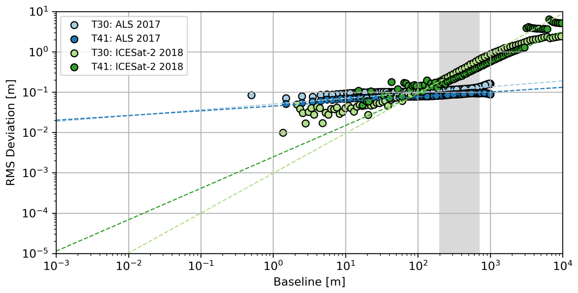
Figure 4 The comparison of March and April 2017 ALS (blues) and November 2018 ICESat-2 (greens) RMS deviation profiles centred on locations T30 (light) and T41 (dark) along the EGIG line. There is a substantial discrepancy between the two sets of RMS deviation profiles in the overlapping baseline range (100 m to 1 km) further confirming that the local regions surrounding T30 and T41 are markedly smoother than those further afield. The anomalous behaviour in the ICESat-2 RMS deviation profiles at both short (i.e., <80 m) and long (i.e., >4 km) baselines is related to the quick drop-off in the number of comparable surface elevations.

In addition to the return of scale-dependent roughness when considering the broader regions surrounding T30 and T41, the ICESat-2 results in Fig. 4 also demonstrate three other notable points. The first is that when the ICESat-2 baseline is pushed to its shortest limit (i.e., considering closely spaced surface elevations at orbit crossovers), the RMS deviation profile appears to flatten. While there are only a small handful of surface elevation measurements at these short baselines (e.g., tens of points separated by 10 m compared to tens of thousands of points separated by 20 m), the ICESat-2 results do seem to exhibit the same less scale-dependent roughness pattern as has been observed in the ALS results (Fig. 2c and d). Again, as with the ALS data, the transition in the RMS deviation profile occurs in the 100 m range. The second notable point is that the piecewise linear, scale-dependent behaviour in the RMS deviation observed in the ALS data between 200 and 700 m baselines (Fig. 2c and d) appears to continue well beyond that range – to upwards of roughly 3 km in the ICESat-2 results. Recall that only ALS data within 1 km of the in situ measurement location underlie the RMS deviation profiles in Fig. 2, limiting the ability to constrain roughness over large baselines with the ALS data. The 200 to 700 m interval used in the projection of the RMS deviation profiles to the radar wavelengths is used solely because it is an interval common to both the ALS and ICESat-2 results. The scale-dependent behaviour in the surface roughness appears to extend to much longer baselines. Lastly, while the ICESat-2 RMS deviation profiles suffer data availability issues, there does appear to be another marked transition to less scale-dependent roughness at the longer (i.e., >4 km) baselines.

4.2 Spaceborne datasets

Turning to the spaceborne altimetry datasets (i.e., ESA CryoSat-2, CNES–ISRO SARAL, and NASA ICESat-2), the first step is to derive RMS deviation profiles from the laser altimetry surface elevations (similar to Fig. 4). To maintain equivalence in the spatial representativeness of the radar and laser altimetry surface roughness metrics for a specific location in the 5 km × 5 km grid, ICESat-2 RMS deviation profiles are derived from all November 2018 surface elevations within the three different RSR surface echo power search radii for that location (maximum search radii are presented in Table 1). The number of ICESat-2 measurements within the location-specific CryoSat-2 LRM, CryoSat-2 SARIn, and SARAL search radii for November 2018 are presented in Fig. 5. As expected, because the spatial density of surface echo power measurements along an individual orbit (and therefore across a month) is greatest for CryoSat-2 when operating in its SARIn mode, the associated smaller search radii contain the fewest ICESat-2 measurements (Fig. 5b). In contrast, the lower spatial resolution (i.e., less frequent along-track sampling) inherent in the CryoSat-2 LRM (Fig. 5a) and SARAL (Fig. 5c) data requires a greater RSR search radius that, in turn, encompasses more ICESat-2 measurements. The cross-cutting striped patterns in Fig. 5 relate to the specific distribution of satellite ground tracks across the GrIS in November 2018. As three different sets of ICESat-2 data are used to derive three RMS deviation profiles for each location, three different background planes are also defined based on the local ATL06 surface elevations.

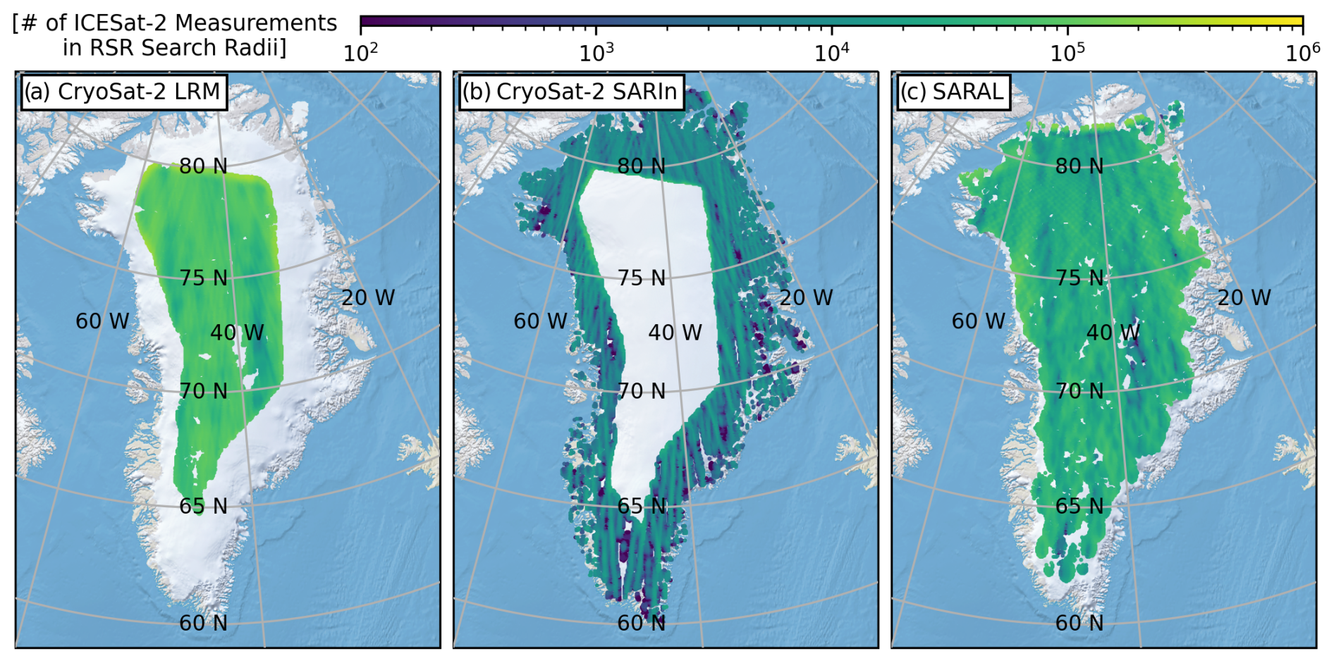
Figure 5 Maps showing the number of November 2018 ICESat-2 ATL06 measurements within the contemporaneous (a) CryoSat-2 LRM, (b) CryoSat-2 SARIn, and (c) SARAL RSR search radii. The quantity of ICESat-2 ATL06 surface elevations used to derive the RMS deviation profile for a specific location is inversely related to the along-track data rates of the different radar altimeters.

In lieu of presenting hundreds of individual ICESat-2 RMS deviation profiles together with the CryoSat-2 and SARAL RMS heights from Scanlan et al. (2023a) (i.e., akin to Fig. 2c and d) and following on from what has been learned from the CryoVEx results, Fig. 6 presents the comparison of those initial RSR RMS height estimates from Eq. (3) and the wavelength-scale RMS deviations projected from a linear fit to the RMS deviation profiles for baselines between 200 and 700 m for 328 locations across the GrIS. As presented in relation to Fig. 4, the 200–700 m interval is selected due to its general representativeness of the piecewise linear, scale-dependent roughness behaviour observed in both the ALS and ICESat-2 data. It should not be considered a uniquely fixed interval. These 328 locations have been pseudo-randomly selected based solely on considerations for the computational load when performing the point-to-point surface deviation comparison as part of the RMS deviation profile calculation (i.e., ≤55 000 ICESat-2 surface elevations). To ease the comparison, all surface roughness estimates (i.e., CryoSat-2 and SARAL RSR RMS heights or ICESat-2 RMS deviations projected to the CryoSat-2 and SARAL wavelength scale) have been normalized by the radar signal wavelength. While there may be the suggestion of a possible linear relationship between the radar- and laser-derived surface roughness estimates, it is clearly not a 1:1 agreement. This appears to be in part due to a floor in the RSR results, as they consistently fail to recover the smallest ICESat-2 RMS deviations. The mean absolute error between the two sets of surface roughness estimates is 0.0308λ for CryoSat-2 and 0.0346λ for SARAL.

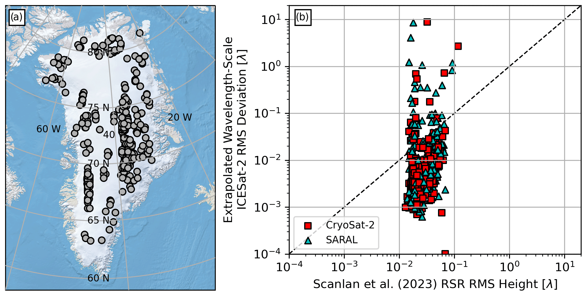
Figure 6 Panel (a) presents the locations of 328 pseudo-randomly chosen locations across the GrIS where in panel (b) Scanlan et al. (2023a) RSR surface roughness results (CryoSat-2 as squares and SARAL as triangles) are compared to wavelength-baseline-projected RMS deviations from ICESat-2. While there is a general positive association between the two sets of roughness estimates, the RSR results do not reliably recover the smallest ICESat-2 roughness levels. The mean absolute errors between the ICESat-2 and the CryoSat-2 and SARAL RSR-based wavelength-normalized roughness estimates are 0.0308λ and 0.0346λ, respectively.

5 Revising the derivation of surface roughness

5.1 An empirical roughness relationship

The clear absence of a good agreement in Fig. 6 between the CryoSat-2 (LRM and SARIn) and SARAL RSR results and – what are taken to be – equivalent results derived from ICESat-2 necessitates a deeper investigation into the rationale for why. As such, building off the general relationship established by Eq. (3), Fig. 7 presents a two-dimensional histogram directly comparing the CryoSat-2 and SARAL coherent to incoherent power ratios (in linear units plotted on a logarithmic axis) with the radar-wavelength-scale RMS deviation projected from the ICESat-2 RMS deviation profile between the 200 and 700 m baselines. Following Fig. 6, the projected ICESat-2 RMS deviations in Fig. 7 have been normalized by the radar signal wavelength to facilitate the joint analysis of the Ku- and Ka-band results. The solid line in Fig. 7 represents the analytical solution for relating the $P_{\mathrm{c}}/P_{\mathrm{n}}$ ratio to surface roughness via the SPM (i.e., Eq. 3) (Grima et al., 2014b). It is immediately clear that the analytical solution does not fit the observed relationship and leads to the surface roughness being almost universally overestimated. However, Fig. 7 does suggest a general association between the RSR $P_{\mathrm{c}}/P_{\mathrm{n}}$ ratio and the wavelength-baseline-projected ICESat-2 RMS deviations. Because this association is linear (when plotted in log–log space), we use it to define the following empirical mapping:

$$\begin{array}{}\text{(5)}& v(\mathit{\lambda }{)}_{\text{ICESat-2}}=\mathit{\lambda }\times {\left({\displaystyle \frac{P_{\mathrm{c}}}{P_{\mathrm{n}}}}\right)}^{-\mathrm{0.892}}\times {\mathrm{10}}^{-\mathrm{1.706}}.\end{array}$$

The overestimation of surface roughness based on the RSR $P_{\mathrm{c}}/P_{\mathrm{n}}$ ratio when using the SPM may seem somewhat disconcerting, knowing its range of validity covers the smallest RMS heights (kσ_h<0.3). However, the SPM assumes scale-independent surface roughness, while, outside of very local areas (e.g., Fig. 3), surface roughness across the GrIS appears strongly scale-dependent (Figs. 1 and 4). As such, the SPM was likely ill-suited to the task of deriving surface roughness from the RSR results from the beginning.

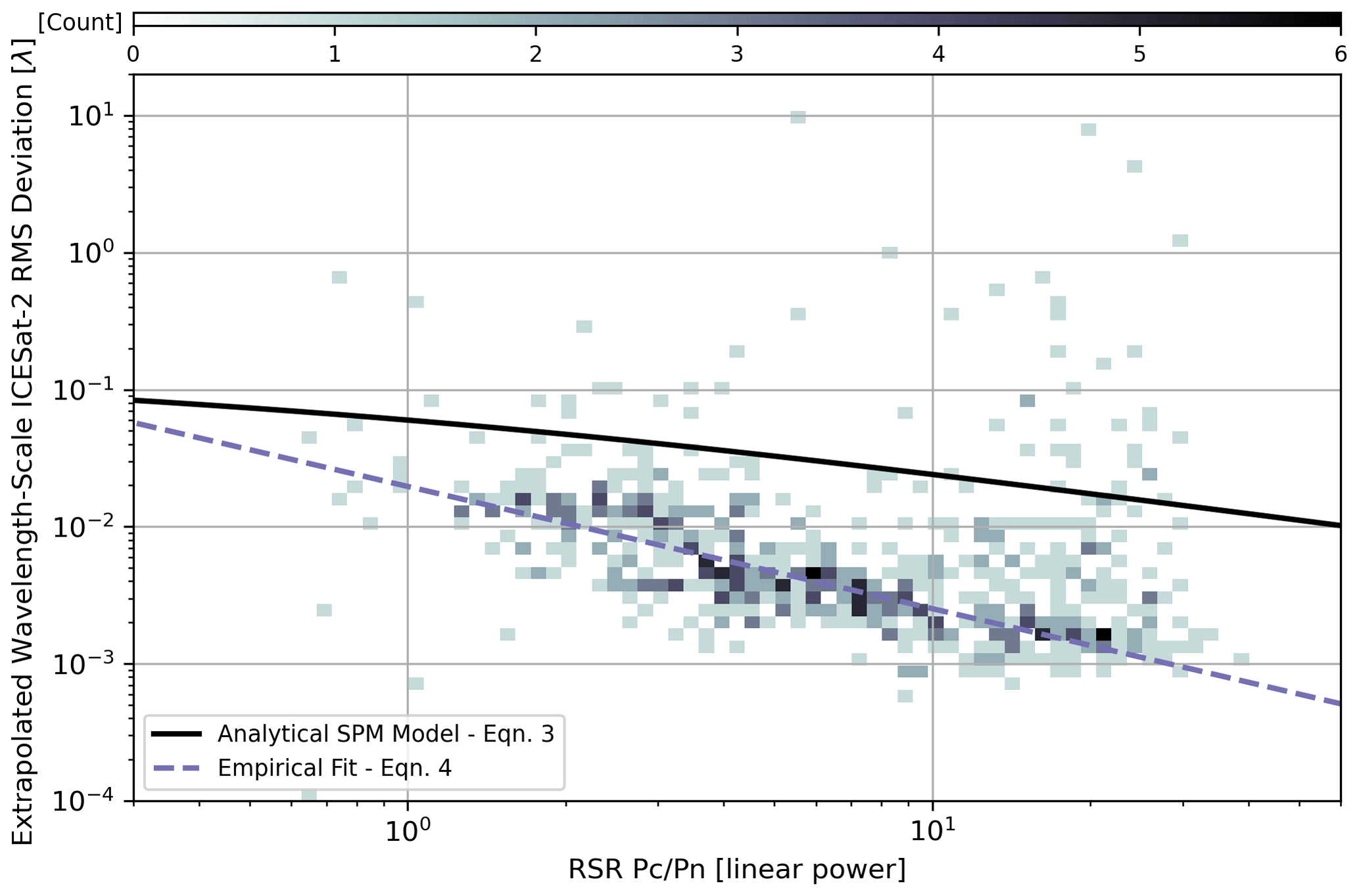
Figure 7 Direct comparison of the combined CryoSat-2 and SARAL coherent to incoherent ($P_{\mathrm{c}}/P_{\mathrm{n}}$) power ratios on which RSR estimates of surface roughness are based and the projection of the ICESat-2 RMS deviation profile between 200 and 700 m baselines to the wavelength scale. As the conventional analytical model (solid line, Eq. 3) leads to overestimating surface roughness, a new linear empirical mapping (dashed line, Eq. 5) is suggested as being more appropriate.

Applying this empirical relationship to deriving surface roughness estimates from the RSR outputs yields the comparison against the projected ICESat-2 RMS deviations presented in Fig. 8. Comparing Fig. 6b and Fig. 8, surface roughness produced using the empirical mapping relation (Eq. 5) clearly produces a better match than the analytical model (Eq. 3). Quantitatively, the mean absolute errors between the ICESat-2 and RSR-based wavelength-normalized roughness estimates are reduced from 0.0308λ (CryoSat-2) and 0.0346λ (SARAL) for the analytical model to 0.0119λ and 0.0174λ using the empirical model, the substantial reduction indicating a much better agreement between the radar and laser roughness estimates. Furthermore, the difference between ICESat-2 and RSR-based empirical surface roughness clusters around zero for both CryoSat-2 (Fig. 8b) and SARAL (Fig. 8c), whereas the analytical approach led to consistently greater RSR surface roughness. A similar study but only with a smaller number of locations in December 2018 also observed an improvement in mean absolute error using the revised empirical RSR roughness model (Eq. 5). Expanding more broadly, the form of Eq. (5) and the procedure for developing it could be adapted to other RSR implementations on Earth as well as beyond, but care will have to be taken to ensure the coefficients are appropriate as they may vary in different contexts/applications.

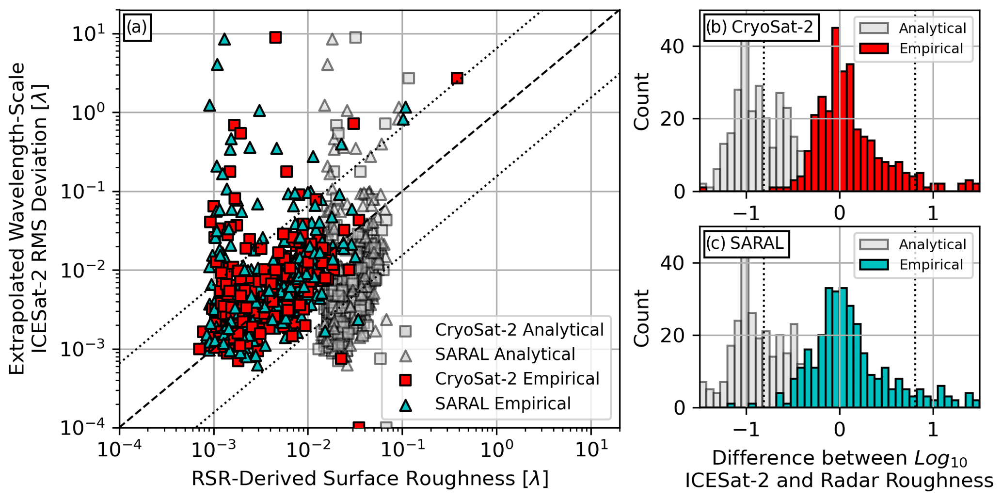
Figure 8 Direct comparison of the empirical and analytical RSR and ICESat-2 surface roughness results (a) and histograms of the differences in the logarithms of ICESat-2 and RSR surface roughness values for (b) CryoSat-2 and (c) SARAL. Using the empirical mapping between the RSR outputs and surface roughness, the mean absolute error is reduced to 0.0119λ and 0.0174λ for CryoSat-2 and SARAL, respectively. The analytical results are the same as those presented in Fig. 6b. The dashed line in (a) represents a 1:1 agreement between the radar and laser surface roughness results, while the dotted lines are used to identify the >2σ outliers in the radar and laser surface roughness estimates.

An interesting feature present in the radar and laser surface roughness comparison of Fig. 8 is that substantial disagreements (i.e., >2σ outliers) between the radar and laser altimetry surface roughness estimates are not symmetric and mainly occur above the dashed 1:1 line (i.e., an ICESat-2 surface roughness greater than that of either CryoSat-2 or SARAL). When looking at where all of these outliers occur spatially across the GrIS (Fig. 9a and b), there is a clear clustering of locations in southeast Greenland. That some outlying surface roughness results can be found around the GrIS periphery or at the boundary of the different CryoSat-2 acquisition modes is not unexpected, as this is where the RSR technique is known to struggle with more spatially heterogeneous surfaces and where there are fewer data enveloping a specific location (Scanlan et al., 2023a). That being said, the cluster in southeast Greenland is surprising as it occurs across a high elevation and inland portion of the ice sheet. Interestingly, the southeast Greenland cluster of roughness mismatches corresponds to a location where monthly (2013–2018) RSR results meeting the quality control criteria (Sect. 3.2) are amongst the rarest. This suggests that the GrIS surface in this area may be unique in some way that continuously affects the RSR results. Based on the ICESat-2 results from Fig. 8, one possible explanation could be that this area is substantially rougher than the inland GrIS as a whole and yields distributions of radar altimetry surface echo powers that cannot be cleanly fit by a single homodyned K-distribution probability density function. Other alternative explanations that could incite changes in the distribution of surface echo powers include a local variation in volume scattering affecting the amount of diffuse scattering and firn crusts/thin layering affecting the specular component. However, as this study focuses on understanding the RSR roughness results, a deeper assessment of the root cause for why the RSR technique seems to experience issues in this area is left to future work.

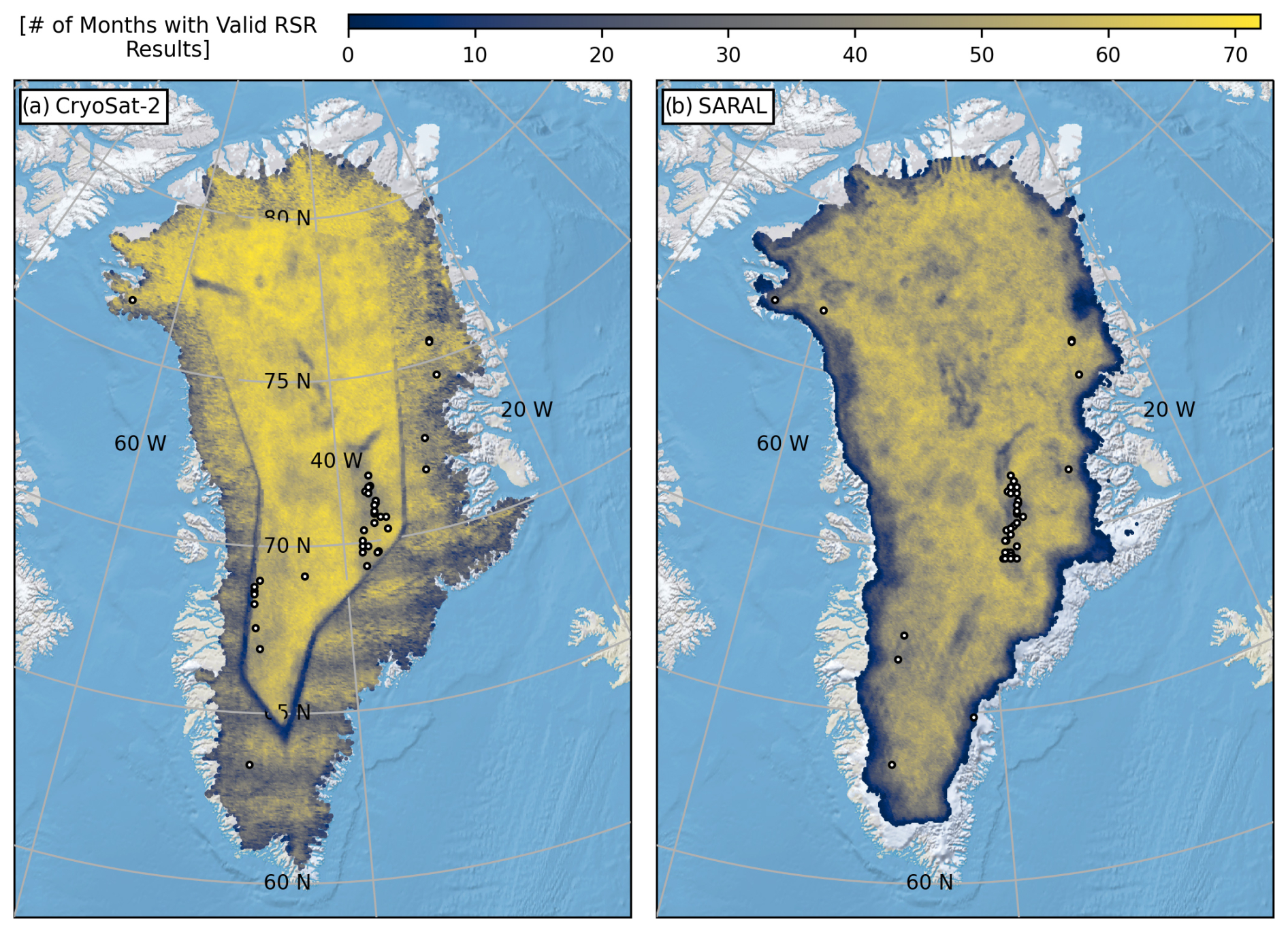
Figure 9 Locations of all >2σ outliers between the wavelength-scale RMS deviations projected from ICESat-2 and (a) CryoSat-2 and (b) SARAL surface roughness estimates. The locations are plotted on top of maps showing the number of months with valid (i.e., quality-controlled) RSR observations for the period 2013–2018 (72 months). While some outlying roughness mismatches occur closer to the boundaries of the various datasets, there is a cluster in southeast Greenland at ∼3000 m elevation in the vicinity of the ice divide that corresponds to a zone of RSR results that do not meet the quality control criteria. The impact of CryoSat-2 and SARAL orbital designs can be seen in the spatial patterns (CryoSat-2 SARIn latitudinal stripping and SARAL hatching) in the southern portions of the ice sheet.

5.2 Spatiotemporal patterns in surface roughness

Armed with an improved understanding of surface roughness derived from analysing Ku- and Ka-band satellite radar altimetry surface echoes, we can now take a closer look at the resulting spatiotemporal patterns. To this end, Fig. 10 presents the 2013–2018 SARAL mean surface roughness (Fig. 10a) as well as time series along two GrIS-bisecting transects: an east–west transect in Fig. 10b and a north–south transect in Fig. 10c. Blank points in the time series (Fig. 10b and c) correspond to instances where the corresponding RSR results have been removed during the quality control step (Sect. 3.2), and these missing data have been neglected in the calculation of the 2013–2018 mean. Note that the southeastern portion of the GrIS, where the RSR method seems to struggle and yields results that do not meet the quality control requirements (Fig. 9), can also be observed along the east–west transect as a horizontal line of missing RSR results at roughly 38° west longitude.

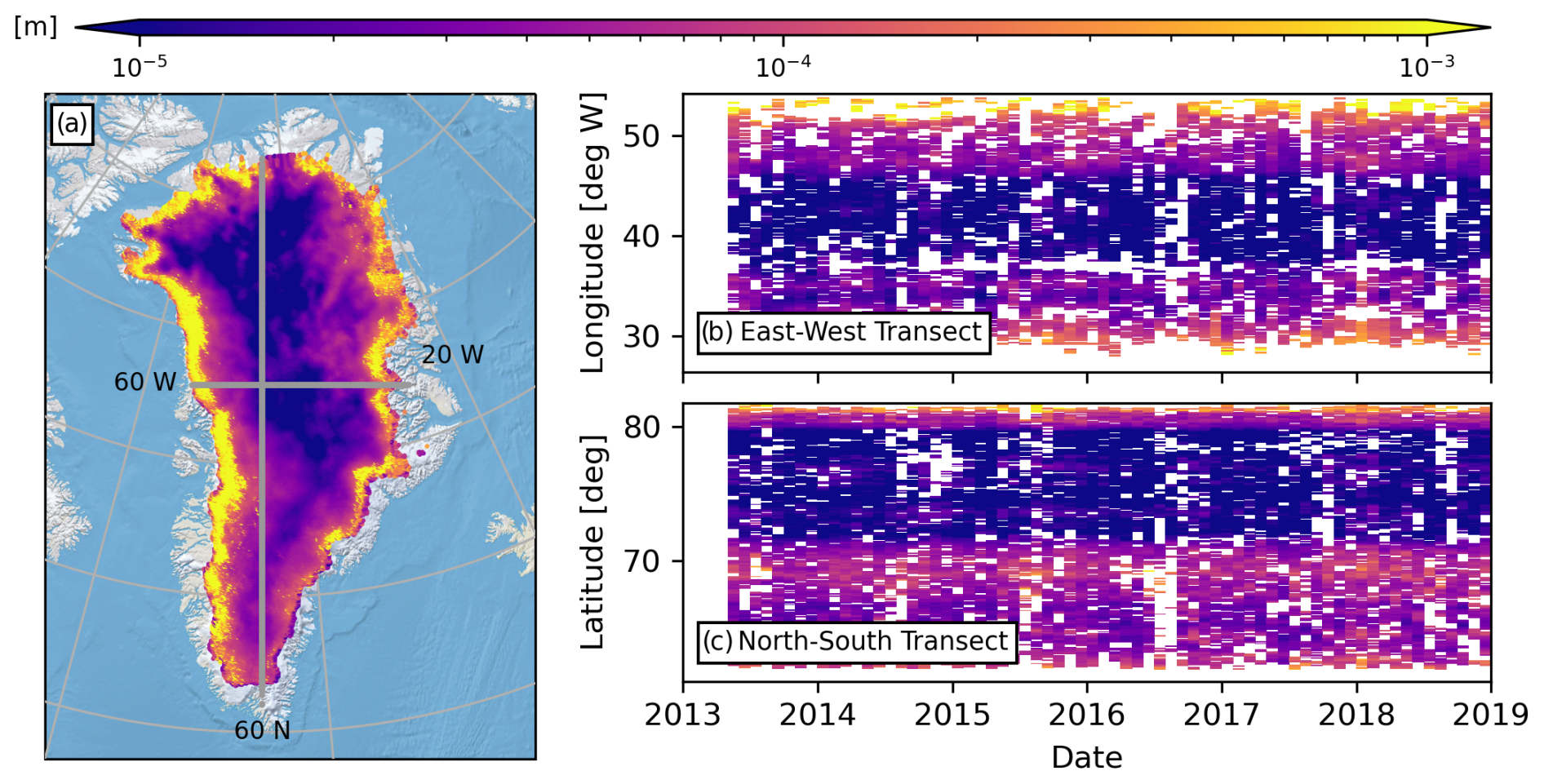
Figure 10 The 2013–2018 SARAL surface roughness mean (a) and time series (b, c) along east–west and north–south transects cross-cutting the GrIS. While there is strong spatial variability in RSR-derived surface roughness across the 6-year period (i.e., margins are rougher than the interior), the temporal variability in surface roughness is minor.

The spatial patterns in surface roughness are similar to those presented in Scanlan et al. (2023a) and highlight the expected pattern of a smooth ice sheet interior that becomes progressively rougher towards the margin and in the south. Elevated surface roughness in the vicinity of the fast-flowing Northeast Greenland Ice Stream (NEGIS) is also clearly discernible. The region of elevated surface roughness further inland from the margin at latitudes slightly less than 70° overlaps with the catchment of Sermeq Kujalleq (Jakobshavn Isbræ). What has changed in these new surface roughness results from those previously published is the more reliable recovery of smaller roughness values that were previously not being captured (Fig. 8). Temporally, surface roughness along these transects exhibits no strong seasonal signal. There are some isolated, small variations in surface roughness (e.g., a minor increase in roughness near 69°N in mid-2015), but overall, surface roughness is strongly consistent through time. This is not surprising when considering the context for interpreting the RSR-derived surface roughness results that was established based on the CryoVEx analysis in Sect. 4.1. It is difficult to envision inducing rapidly repeating (e.g., annual) changes in the roughness of the GrIS surface over horizontal baselines that are hundreds of metres long (i.e., those the RSR results seem to be projections of). Changes in roughness over these horizontal scales likely take place over longer timescales.

6 Relevance and implications of RSR-derived surface roughness

6.1 Implications for SMB and heat flux modelling

As introduced previously, surface roughness is considered an important component in SMB and heat flux modelling studies. It is typically used as an input in the calculation of either the aerodynamic roughness length or the similar drag coefficient metric. Even though it is termed a “roughness”, the aerodynamic roughness length is conceptually different from how roughness is considered in the context of this study (i.e., a statistical description of the undulations in surface heights) as it quantifies the height above the ground surface at which the horizontal wind-speed profile is zero. The use of the aerodynamic roughness length and drag coefficient metric varies in practice: Jakobs et al. (2019) employ the aerodynamic roughness length as a free model tuning parameter. Amory et al. (2016) provide no direct quantifiable link between the drag coefficient and a description of surface roughness, only implying that the drag coefficient is impacted by the small-scale distribution of sastrugi. In contrast, Smeets and van den Broeke (2008) and van Tiggelen et al. (2023) incorporate the assumed average hummock height in their derivation of the aerodynamic roughness length across the GrIS ablation zone. In a more quantitative study based on airborne photogrammetry and spaceborne ICESat-2 laser altimetry, van Tiggelen et al. (2021) uses the standard deviation of a low-pass-filtered (<35 m wavelength), high-resolution (1 m horizontal sampling) elevation profile to derive the aerodynamic roughness lengths over the K transect. The overarching implication from all these studies is that it is the highly localized, individual surface roughness features that exert the dominating influence on the energy flux at the ice sheet surface. It is therefore the statistical descriptions of the undulations of these individual features (i.e., average height, standard deviation of heights) that then feed into GrIS SMB models.

Our validation of RSR-derived SARAL and CryoSat-2 surface roughness against CryoVEx and ICESat-2 laser altimetry shows that the assumption of scale-invariant surface roughness from Scanlan et al. (2023a) is ill-suited for broad regions of the GrIS. Furthermore, the RSR-derived surface roughness appears to lie below the continued projection of the RMS deviation profiles to the SARAL and CryoSat-2 radar wavelength scale (Fig. 2), a fact that would not have been recognized had the CryoVEx ALS data not been used to reliably recover RMS deviations at baselines shorter (e.g., < 40 m) than are typically recoverable from ICESat-2 ATL06 surface heights outside of orbit crossovers (Fig. 4). Had this analysis relied solely on ICESat-2 heights, the RSR surface roughness results would have been mistakenly interpreted as the true wavelength-scale RMS deviations (Fig. 8). Instead, for the Ku- and Ka-band airborne and satellite radar altimetry data, RSR surface roughness is best interpreted not as the true wavelength-scale RMS deviation but as the projection of the scale-dependent behaviour observed at baselines between hundreds of metres and a few kilometres to the wavelength scale. The implication is then that the SARAL and CryoSat-2 RSR surface roughness results only have physical meaning far beyond the individual roughness feature scales currently considered critical in heat flux and SMB studies. As such, they have no direct role to play in the improvement of current GrIS SMB modelling. The relevance only at long baselines is likely also the reason why the surface roughness time series presented in Fig. 10 do not exhibit the strong seasonal variability that has been reported in derivations of aerodynamic roughness lengths (Smeets and van den Broeke, 2008; van Tiggelen et al., 2021, 2023).

Taking a broader view of all the airborne and satellite altimetry (i.e., radar and laser) datasets analysed in this study, they all point to GrIS surface roughness being, at least for some baselines (e.g., 200 m to 3 km), scale-dependent. While there are isolated local areas where roughness is not strongly dependent on the horizontal distance over which it is measured (e.g., immediately surrounding T30 and T41 in Figs. 2–4), when considering the broader regional conditions, scale-dependent roughness appears commonplace (as implied by Figs. 7 and 8). This challenges current SMB models that incorporate surface roughness via a single spatially homogeneous value (e.g., the aerodynamic roughness length). An avenue for future research is then to integrate the effects of scale-dependent roughness into numerical SMB and heat flux models and assess their predictions of ice sheet evolution against reality. At this point, the roughness results derived from the RSR analysis of CryoSat-2 and SARAL surface echo powers will likely have more direct applicability. It should be noted that quantifying surface roughness at the scale of individual features (e.g., sastrugi, hummocks) will be challenging for standard satellite measurements (e.g., ICESat-2 ATL06 land heights; Fig. 4) and that integration with more specialized analyses or alternative datasets (e.g., lidar, UAV photogrammetry) is likely to be required (van Tiggelen et al., 2021).

Even though the RSR surface roughness results do not appear to be relevant as direct inputs for current SMB modelling, this does not mean they are without future intrinsic value by themselves. First, there may be a role for directly using the radar-derived surface roughness estimates to refine the retracking of the radar waveforms and improving surface height determinations. Second, there are clear spatial heterogeneities in the RSR results (Figs. 8 and 9) that warrant further investigation and may shed light on the nature of GrIS surface conditions. Third, they represent a baseline for interpreting the RSR results in the context of other radar backscattering models (Fung and Chen, 2004; Ulaby et al., 1982) and revisiting some of the underlying decisions (e.g., correcting echo powers for nadir slopes prior to RSR processing). Lastly, the ever-increasing confidence in our ability to reliably observe GrIS surface properties from CryoSat-2 and SARAL surface echo powers provides a foundation to continue applying and adapting these techniques to earlier satellite remote sensing datasets (e.g., ERS-1, ERS-2, ENVISAT), thereby extending our observational time series.

6.2 RSR-derived dielectric permittivity

Just as important as the surface roughness results themselves, revising the approach for calculating surface roughness from the coherent–incoherent power ratios will likely have a knock-on effect on the dielectric permittivities (and surface densities) also derived from the RSR results. This is because the impact of surface roughness is included in an adjustment term [$e^{-\left(\mathrm{2}k{\mathit{\sigma }}_{\mathrm{h}}^{\mathrm{2}}\right)}$] applied to the specular scattering equation (Eq. 4) that relates coherent power to the Fresnel reflection coefficient of the surface (Grima et al., 2012, 2014b; Scanlan et al., 2023a). To that end, Fig. 11 presents two-dimensional histograms comparing November 2018 analytical and empirical relative dielectric permittivity estimates from across the GrIS for each radar altimetry dataset (i.e., CryoSat-2 LRM, CryoSat-2 SARIn, and SARAL). As each analytical–empirical comparison result falls just below the dotted 1:1 line, Fig. 11 highlights a slight decrease in dielectric permittivity due to the revised empirical derivation of surface roughness for each radar dataset. However, there is still a very consistent overall agreement between the two sets of permittivity estimates indicative more of a systematic adjustment in the results than a broader re-organization of spatial patterns. Individually, the variability in the analytical–empirical comparisons in Fig. 11 increases from CryoSat-2 LRM (Fig. 11a), to SARAL (Fig. 11c), and to CryoSat-2 SARIn (Fig. 11b), following the degree to which the underlying datasets cover the rougher GrIS margin.

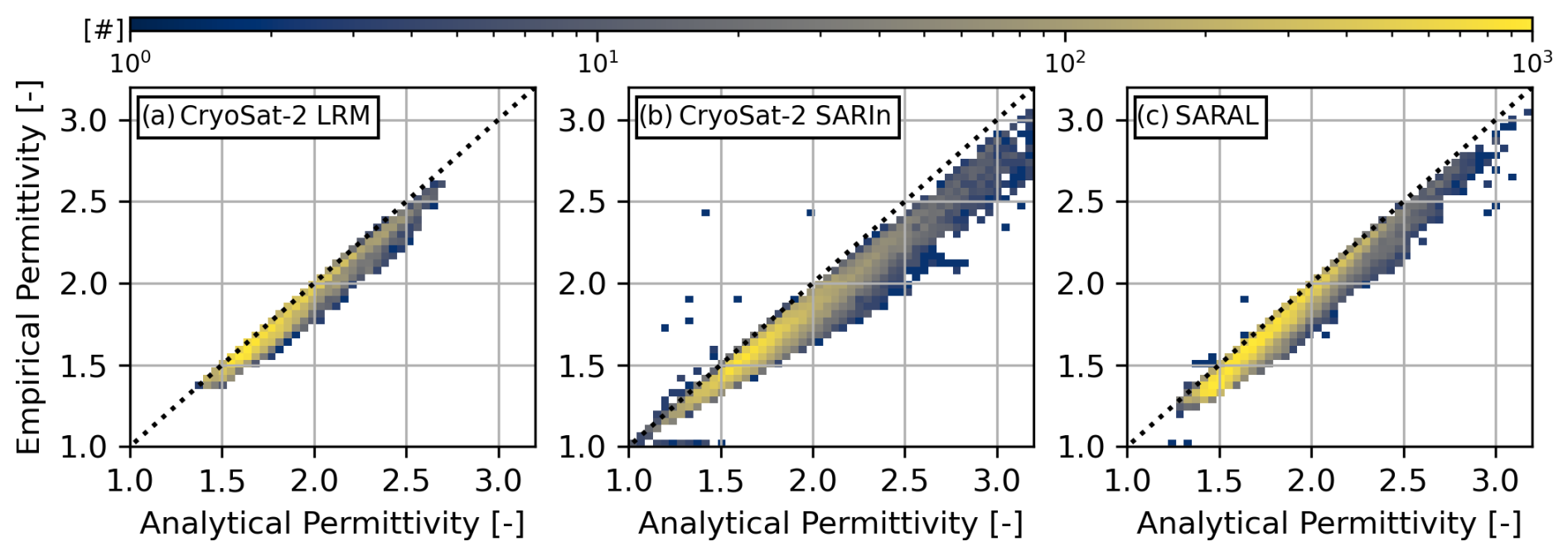
Figure 11 Two-dimensional histograms demonstrating the impact of using the revised empirical model for calculating surface roughness from the RSR results on (a) CryoSat-2 LRM, (b) CryoSat-2 SARIn, and (c) SARAL permittivities. Permittivities are slightly reduced in the empirical results due to the improved recovery of smaller surface roughness values.

Based on Figs. 7 and 8, it is not unsurprising that the analytical permittivities are larger than empirical results. For the same coherent power (P_c) output from the RSR analysis, a stronger Fresnel reflection coefficient (i.e., greater permittivity contrast) is required to overcome the quantitatively larger reduction in coherent power associated with overestimated analytical roughness values (Fig. 8). As the empirical mapping (Eq. 5) more reliably recovers smaller roughness values, the roughness adjustment applied to the RSR P_c output is smaller, and the corresponding permittivity contrast is reduced. That the shift in permittivity between the analytical and empirical results is small speaks directly to the dominantly specular nature of the GrIS in terms of backscattering normal-incidence Ku- and Ka-band radar signals. Now that the surface roughness results are more reliably being derived, a deeper investigation into the revised dielectric permittivities and their relevance to improving our understanding of GrIS surface density evolution will be the central focus of a follow-on study.

6.3 Revisiting laser altimetry as an objective dataset

Throughout this study, the ALS and ICESat-2 laser altimetry data and derived surface roughness results are considered the objective standard against which the radar altimetry RSR-based results are assessed. However, it is also worthwhile to revisit this assumption, as the nuances in the underlying datasets may affect their relative sensitivity to surface roughness conditions.

First consider the scale of the footprints relative to the RMS deviation baselines. For the airborne CryoVEx data, the footprints of individual altimetry measurements are on the order of 0.7 m in diameter (ALS), 3 m along-track by 10 m across-track (ASIRAS), and 5 m along-track by 12 m across-track (KAREN) (Skourup et al., 2019, 2021). The satellite data, on the other hand, as expected have larger footprint diameters ranging between 17.5 m for ICESat-2, 1.65 km for CryoSat-2 (pulse-limited footprint; 720 km altitude, 320 MHz bandwidth), and 1.4 km for SARAL (pulse-limited footprint; 800 km altitude, 500 MHz bandwidth) (Markus et al., 2017; Steunou et al., 2015; Wingham et al., 2006). As the ALS and ICESat-2 footprints are generally smaller than the posting interval for their individual datasets (i.e., 1 m by 1 m for ALS, 20 m along-track for ICESat-2 ATL06), their RMS deviation profiles are assumed to be unbiased over the baselines considered (i.e., smallest roughness baseline is greater than an individual footprint). The sole exception to this though is at crossovers where the laser (ALS or ICESat-2) has sampled the same location multiple times. Examples for the ALS are T12 and T30 in 2017 and T21 in 2019. Laser data are analysed spatially as opposed to by individual CryoVEx segment or ICESat-2 orbit number, so overlaying multiple measurements on top of one another can lead to surface elevation measurements spaced less than one footprint apart. Note though that this will only affect the smallest RMS deviations such as those for a 0.5 m baseline reported in Fig. 2 and <20 m ICESat-2 baselines in Fig. 4. At larger baselines, the individual laser surface heights will continue to be more than one footprint apart and the subsequent RMS deviation profiles should not be biased by any unaccounted for large spatial sensitivities.

Expanding beyond individual footprints to consider coverage, only for the CryoVEx case do the 100 m wide ALS swaths cover the ASIRAS and KAREN radar footprints completely. In this case, it is then possible to be relatively certain that both datasets are responding to the same surface conditions. The same cannot be said for the satellite datasets. In general, the ICESat-2 surface elevations are predominantly sensitive to along-track conditions. While there are ideally surface elevations from all six of the across-track beams (subject to ICESat-2 data quality control; see Sect. 2.2), the spatial sampling of surface roughness will always be denser in the along-track direction. The RSR results, on the other hand, represent the collected response of all scatterers within the broader illuminated radar footprint (Grima et al., 2012, 2014b, 2022). Even though attempts have been made to ensure that the satellite laser and radar data being compared come from the same region (e.g., Fig. 5), the sampling of the surface within those regions is not necessarily equivalent. ICESat-2 RMS deviations will be more strongly affected by any anisotropic surface conditions, whereas the CryoSat-2 and SARAL RSR results are based on a more complete two-dimensional view of the surface. Considering data on a monthly time interval further negates possible impacts of the different orbital designs and repeat cycles (91, 369, and 35 d for ICESat-2, CryoSat-2 and SARAL, respectively).

In summary, while biases stemming from non-negligible laser footprints are considered minimal and care is taken to ensure overlapping measurements for each comparison, the different spatial footprints and sensitivities to anisotropy may still influence surface roughness derived from laser datasets and its comparison to the radar results.

7 Conclusions

Surface roughness is an important parameter to quantify when evaluating how the Greenland Ice Sheet responds to a changing climate as it affects the efficiency of heat transfer from the atmosphere, steers meltwater, and impacts conventional measurements of ice sheet volume change. In this study, we perform a detailed investigation into a new type of surface roughness estimate derived from the Radar Statistical Reconnaissance (RSR) analysis of Ku- and Ka-band airborne (2017 and 2019 CryoVEx campaigns) and satellite (November 2018 CryoSat-2 and SARAL measurements) surface echo powers by comparing them to contemporaneous lidar (airborne) and ICESat-2 (spaceborne) laser surface elevations. Our results demonstrate that, outside of some specific local areas, Greenland Ice Sheet surface roughness is scale-dependent, with surface roughness increasing when quantified over larger baselines (i.e., horizontal distances) in a piecewise pattern. It is therefore important to consider surface roughness quantified over multiple scales. Against this backdrop, surface roughness values derived from CryoVEx radar altimetry surface echo powers do not align with a continuation of the lidar RMS deviation profiles to the wavelength scale. In fact, they appear to align much better with the extrapolation of the consistent piecewise linear portion of the RMS deviation profiles for baselines between hundreds of metres and a few kilometres. Building on the CryoVEx results, the direct comparison between extrapolated ICESat-2 surface roughness RMS deviations (from the piecewise linear portion between 200 and 700 m) and previously published CryoSat-2 and SARAL radar surface echo powers derived using an analytical backscattering model reveals that the radar-based results tend to overestimate surface roughness. In response, a new empirical approach is defined to map the RSR analysis outputs (the coherent-to-incoherent power ratio) to surface roughness. The result is both a marked improvement in the agreement between radar and laser roughness values as well as a greater dynamic range in surface roughness across the Greenland Ice Sheet, further emphasizing the transition from a smooth ice sheet interior to a rougher margin.

The observed sensitivity of the spaceborne RSR results to surface roughness that is, at its smallest, hundreds of metres in scale suggests they are not well-suited to being incorporated in current surface mass balance (SMB) modelling as these models rely on the roughness of individual metre-scale features such as hummocks or sastrugi. However, the glaciological relevance of the RSR-derived surface roughness results is only just beginning to be understood. Future work will focus on investigating if these results can be integrated into waveform retracking and ice sheet height estimations, detecting and mapping regional changes in ice sheet surface behaviour, and applications for earlier remote sensing datasets to expand the current time series. Just as important, the revised empirical approach for estimating surface roughness from radar altimetry surface echo powers yields a decrease in the simultaneously derived surface permittivities – a critical piece of information for follow-on studies targeted at understanding the observational trends in Greenland Ice Sheet surface density. Altogether, this study provides key, fundamental insight into the derivation of Greenland Ice Sheet surface properties from radar altimetry surface echoes as well as the specific context for how the roughness values should be interpreted.