Spatiotemporal patterns of accumulation and surface roughness in interior Greenland with a GNSS-IR network

The dry-snow zone is the largest region of the Greenland Ice Sheet, yet temporally and spatially dense observations of surface accumulation and surface roughness in this area are lacking. We use the global navigation satellite system interferometric reflectometry (GNSS-IR) technique with a novel, low-cost GNSS network of 12 stations in the vicinity of the ice sheet summit to reveal temporal and spatial patterns of accumulation of the upper snow layer. We show that individual measurements are highly precise (±2.8 cm), while the aggregate of hundreds of daily measurements across a large spatial footprint can detect millimeter-level surface changes and is biased by $-\mathrm{2.7}\pm \mathrm{3.0}$ cm compared to a unique validation data set that covers a similar spatial extent to the instrument sensing footprint. Using the validation data set, we find that the reflectometry technique is most sensitive to the surrounding 4–20 m of the surface, with the GNSS antenna at a height of 1–2 m above ground level. Along with an exceptionally high accumulation rate at the beginning of the study, we also detect an across-slope dependence in accumulation rates at yearly timescales. For the first time, we also validate GNSS-IR sensitivity to meter-scale surface heterogeneities such as sastrugi, and we construct a time series of surface roughness evolution that suggests a seasonal pattern of heightened wintertime roughness features in this region. These surface accumulation and roughness measurements provide a novel data set for these critical variables and show a statistically significant relationship with occurrences of both high winds and precipitation events but only moderate correlations, suggesting that other processes may also contribute to accumulation and enhanced surface roughness in the interior region of Greenland.

1 Introduction

The surface mass balance (SMB) of the Greenland Ice Sheet is a key indicator of its response to a dynamic climate: with an acceleration of summertime melt and overall surface mass loss, sea levels are directly impacted (van den Broeke et al., 2016; Smith et al., 2020). In central Greenland, the SMB is still largely positive, but the patterns of accumulation in this region play a critical role in the stability and the evolution of the ice sheet (e.g., McConnell et al., 2000). Quantifying accumulation and its meter-scale variability (closely linked to surface roughness) is an important part of tracking SMB, and an understanding of these variables is also important for assessing stratigraphic noise in ice core interpretations (van der Veen and Bolzan, 1999), determining turbulent heat fluxes over the ice sheet (van Tiggelen et al., 2021), modeling firn gas exchange (Albert and Hawley, 2002), and validating space-borne radar (Scanlan et al., 2023). Meanwhile, the drivers of accumulation and surface roughness in the dry-snow zone, such as precipitation, sublimation, and wind erosion, are hard to measure given temporally and spatially sparse ground-based observations, complicating the formulation of a process-level understanding of accumulation (Castellani et al., 2015).

The few long-term measurements of accumulation or surface roughness in central Greenland commonly sacrifice some aspect of spatial or temporal scale: for example, ice cores provide a record of accumulation and climatic patterns over long timescales but no present-day information. On their own, cores are point measurements in space and therefore reveal little in terms of locally varying processes such as wind erosion (Kuhns et al., 1997). As such, factors including spatially and seasonally varying accumulation must be understood in order to quantify the stratigraphic noise in ice cores (Fisher et al., 1985). To better interpret ice core records and connect them with modern surface processes, near-real-time studies have been established on the ice sheets: for example, stake fields in the vicinity of coring sites can better capture the modern spatially varying accumulation signal, with measurements often made on weekly or yearly scales (e.g., Dibb and Fahnestock, 2004). However, snow stakes are manual measurements and therefore pose logistical constraints, while approximations must be made to convert surface height measurements to accumulated water equivalent volume (e.g., Takahashi and Kameda, 2007). A more recent method that circumvents this gap uses a buried cosmic-ray counter to directly quantify the surface mass balance (Howat et al., 2018). Although this method addresses the aforementioned shortcoming with the snow stake method in converting heights to mass, this technique may still be limited in its spatial footprint. Lastly, remotely sensed surface height change, such as with the ICESat-2 laser altimeter, can provide ice-sheet-wide coverage, while temporal gaps and its spatial resolution make studying small-scale surface processes difficult (van Tiggelen et al., 2021). As such, there remains an opportunity to provide measurements at higher temporal resolution and duration, along with greater spatial representativeness for a given area of study.

Here, we leverage a network of precise, easily deployable, low-cost global navigation satellite system (GNSS) instruments that were positioned for 2 years over tens of kilometers to expand both spatial and temporal measurements of surface accumulation and surface roughness. To retrieve surface measurements, we employ GNSS interferometric reflectometry (GNSS-IR), whereby the direct and reflected signals from GNSS satellites incident upon the GNSS receiver antenna create a characteristic signal-to-noise ratio (SNR) interference pattern that directly corresponds to the antenna height above the snow surface (Larson et al., 2009). Unlike point measurements of the snow, GNSS-IR can sense a large area (∼ hundreds to thousands of square meters) due to the azimuthal distribution of reflected GNSS signals about the instrument, and this method can produce a temporally dense or even continuous series of surface measurements depending on the logging configuration of the receiver. This technique has been used in other studies to measure accumulation throughout the cryosphere, such as in alpine environments (Larson, 2016; Wells et al., 2024), on the Greenland Ice Sheet (Larson et al., 2020; Dahl-Jensen et al., 2022), and in Antarctica (Siegfried et al., 2017; Shean et al., 2017; Pinat et al., 2021).

With our GNSS network, we examine not only the time series of the 24 h mean surface height at each station but also the surface height variability at each individual station and between each station. While these aforementioned GNSS-IR studies produce singular height averages during a certain time period, we extend the GNSS-IR technique by evaluating the spatial heterogeneities (roughness) within the instrument sensing footprint. The time series of surface roughness addresses a critical gap in cryosphere observations of small-scale surface roughness evolution through time. Together with accumulation measurements, we can take advantage of the temporal and spatial resolution of these data to link patterns of accumulation and roughness with precipitation and winds.

This paper is organized as follows: firstly, we provide information on the GNSS network, instrumentation, and auxiliary data, along with background on the GNSS-IR technique and its spatial properties. Next, we statistically validate the GNSS-IR technique by comparing surface height measurements with a long-running snow stake field of similar spatial extent, being the first study to our knowledge to assess GNSS-IR-derived measurements with those made over a comparable footprint in the cryosphere. We also extend this analysis by determining the precision of individual GNSS-IR measurements and evaluating any differences between L1 and L2 GNSS frequencies. Then, we assess the GNSS-IR technique in quantifying surface roughness that arises from heterogeneities in local accumulation. Finally, we analyze the daily, seasonal, and spatial patterns of accumulation and surface roughness derived from this technique and connect these measurements to occurrences of high winds and precipitation.

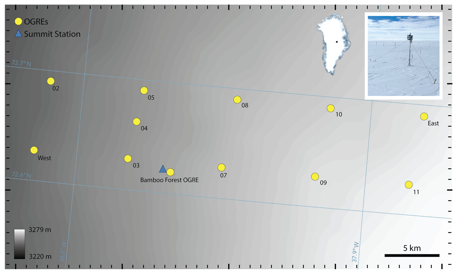
Figure 1 Open GNSS Research Equipment (OGRE) array in the Summit vicinity. The background shading highlights the elevation from the ice divide to the west and is derived from the MEaSUREs Greenland Ice Mapping Project 2 (Howat et al., 2014). Inset: example OGRE setup with the GNSS antenna, instrument, and solar panel mounted on a pole ∼2 m above ground and with the battery buried just below the surface. This particular instrument was placed in the Summit Station Bamboo Forest, an 11-by-11-stake array covering a similar area to the OGRE sensing footprint.

2 Instruments and methods

2.1 Open GNSS Research Equipment (OGRE) network

The network of 12 GNSS stations spans a 35 km east–west transect in the Summit Station vicinity of the Greenland Ice Sheet, with the easternmost stations positioned near the ice divide (Fig. 1). These stations were originally deployed to record surface velocity, validate ICESat-2 laser altimetry height estimates of the ice sheet, and demonstrate the utility of low-cost, high-precision instruments in the cryosphere, and here we use them to analyze accumulation patterns in the network area using the GNSS-IR technique. Each station is built from a low-cost, low-power instrument called Open GNSS Research Equipment (OGRE), designed specifically for rapid overwinter deployments (Pickell and Hawley, 2024b). The OGRE is built on a u-blox ZED-F9P multi-band, multi-GNSS chip. Station configuration includes a lightweight u-blox ANN-MB patch antenna mounted on a 3 m pole, a 10 W solar panel with the instrument mounted on the back side, and a 40 A h battery buried below the surface to minimize drifting. Most stations recorded 1 Hz data for 24 h periods once, twice, or 4 times monthly, year round, to coincide with ICESat-2 overpasses, and the Bamboo Forest OGRE recorded 24 h data once weekly. Due to a chip shortage during the fabrication of these instruments, three stations (West, 07, 09) were built with a sister chip that tracks GNSS satellites at L1 and L5 frequencies instead of L1 and L2; we do not analyze the L5 signals in this paper.

2.2 MERRA-2 atmospheric reanalysis product

We use NASA's Modern-Era Retrospective analysis for Research and Applications, Version 2 (MERRA-2), for the synoptic variables in this study (Global Modeling And Assimilation Office and Pawson, 2015). Due to the intermittency of meteorological data during the winter of 2022 at Summit Station, we chose to use MERRA-2 for the timing and magnitude of wind and precipitation events as part of our surface process analysis. MERRA-2 and other reanalysis products provide reliable near-surface climatic conditions (e.g., Wang et al., 2019; Gossart et al., 2019), but, in ice sheet environments, biases may still exist: MERRA-2 is shown to underestimate precipitation and evaporative processes that lead to surface accumulation (Siegfried et al., 2017; Howat, 2022). MERRA-2 variables are linearly interpolated to each of the OGRE station locations.

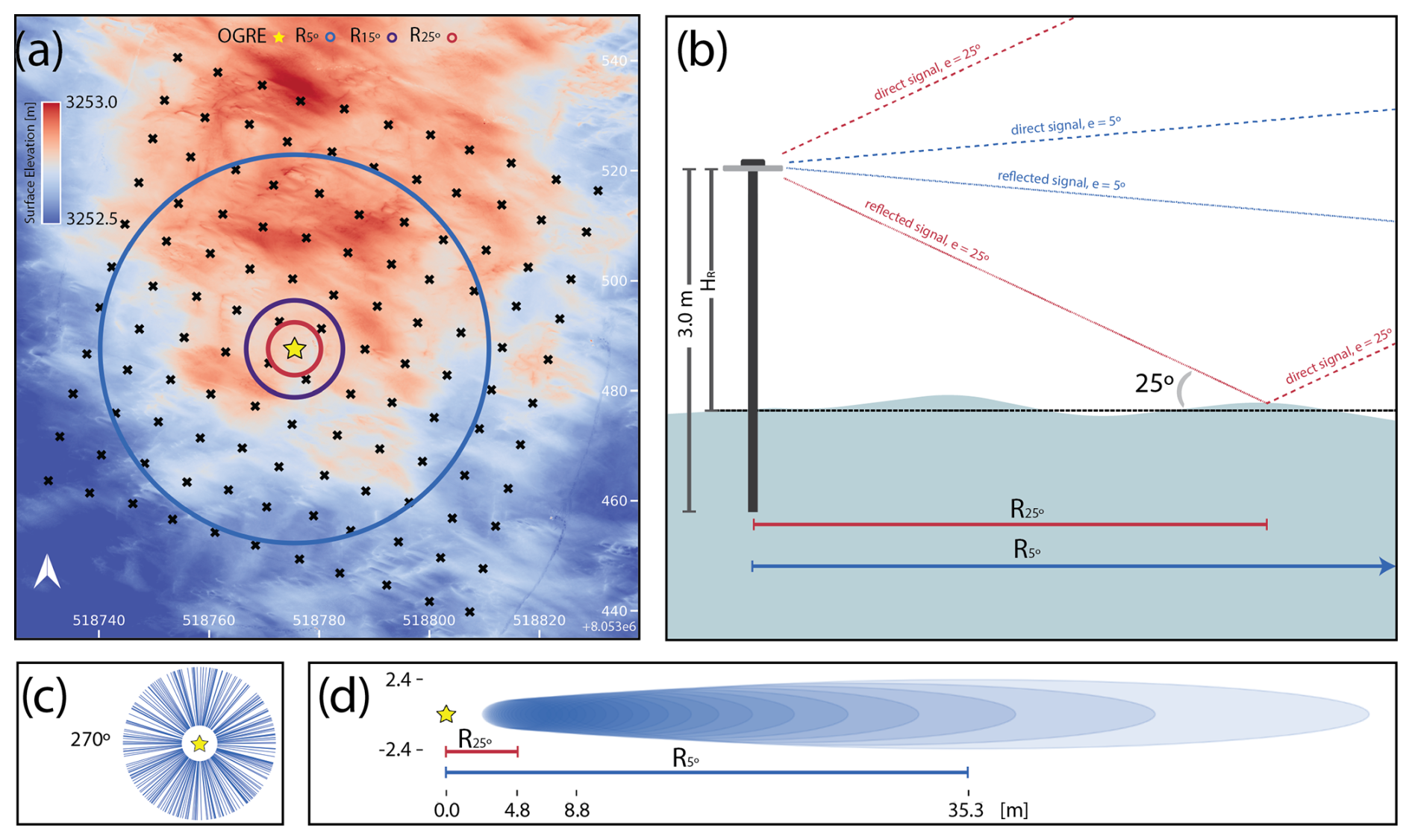
Figure 2 (a) Plan view of Bamboo Forest OGRE, projected into WGS 84/UTM zone 24N. The reflection points corresponding to satellite elevations of 5, 15, and 25° are drawn radially about the OGRE (calculated based on a 2 m antenna height) in blue, purple, and red, respectively. This OGRE is located in the Bamboo Forest, a 121-accumulation-stake network which we used to validate GNSS-IR. The background is the TLS-derived surface elevation from 16 June 2024. (b) Elevation view of OGRE antenna and GNSS-IR reflection geometry, showing the antenna mounted on a partially buried 3.0 m pole (instrument not shown). As a GNSS satellite rises (or sets) through the elevation range of 5 to 25°, the location of the surface reflection point changes from a maximum radial distance from the antenna at 5° to a minimum distance at 25°. (c) Plan view of the locations of all observed satellite arcs from the perspective of the OGRE over a 24 h period on 18 August 2022. (d) Detailed plan view of the L1 frequency Fresnel zone geometry of a single satellite arc from panel (c) relative to the OGRE, with the reflecting signal ellipse center point labeled at satellite elevation angles corresponding to R=5° and R=25°.

2.3 Snow stake array

The snow stake array, also referred to as the “Bamboo Forest”, is arranged in an 11-by-11-stake grid with each stake spaced approximately 8 m apart (80 m by 80 m). The array is located east of Summit Station in a region of relatively undisturbed snow, and the grid is rotated approximately 15° clockwise from true north to align with the prevailing winds (Fig. 2a). Measurements are made on a weekly basis when weather conditions allow, and data have been collected since 2003. Heights from a fiducial mark on each stake are made to the snow surface and are sensitive to the same snow surface height change as measured by the OGRE stations with GNSS-IR. One of the OGREs is located within the Bamboo Forest (“Bamboo Forest OGRE”) and programmed to log once weekly on Wednesdays, the target day of the manual Bamboo Forest survey.

As each stake height measurement is unreferenced to all others, we surveyed the Bamboo Forest with an automatic level on 14 June 2024 to reference all stakes and the Bamboo Forest OGRE to the same horizontal reference datum. This allows the direct comparison of the biases between the Bamboo Forest stakes and the Bamboo Forest OGRE. The snow surface in the Bamboo Forest was also scanned with a VZ-2000i terrestrial laser scanner (TLS) on 16 June 2024 for further intercomparison and spatial analysis of the OGRE data at 10 cm horizontal spatial resolution (Fig. 2a).

2.4 Surface height change and GNSS-IR technique

Surface height is the distance from the antenna phase center on the OGRE or the fiducial mark on the bamboo stakes to the snow surface. In the GNSS-IR literature, this value is commonly called the reflector height (H_r) to indicate that the measurement is the vertical height from the reflecting surface (snow–air interface) to the antenna phase center. We adopt this nomenclature when referring to the OGRE antenna heights above the surface. Changes in H_r are sensitive to several processes in the dry-snow zone (Castellani et al., 2015):

$$\begin{array}{}\text{(1)}& \mathrm{\Delta }{H}_{\mathrm{r}}=P+M+L+C+W,\end{array}$$

where P is precipitation as snowfall, M is melt (generally negligible at Summit), and L is surface change due to latent heat flux and can be positive or negative if in a depositional regime or a sublimation regime, respectively, depending on atmospheric conditions. C is compaction between the surface and the bottom of the pole, and we assume the pole to be locked into the layer at its base per Takahashi and Kameda (2007). Finally, W is wind redistribution, which can also be positive (depositional) or negative (erosional). In this paper, we also refer to ΔH_r as “accumulation”, which can be positive or negative and represents the change in the snow layer between the measured surface and the anchored bottom of the pole.

In calculating H_r, GNSS-IR does not rely on any position-related measurements made by the instrument; instead, the only data of interest are the SNR levels measured by the instrument for each satellite signal. When tracking satellites at low elevation angles, the gain characteristics of a zenith-pointing GNSS antenna are such that they are susceptible to not only the direct incoming satellite signal but also any reflected signal, called multipath (Fig. 2b). At the antenna phase center, these signals interfere, and whether they do so constructively or destructively at a given satellite elevation angle is a function of antenna height above the reflecting surface. Specifically, the frequency of the interference pattern as the satellite rises is directly related to the ratio of the antenna height and the signal wavelength (Georgiadou and Kleusberg, 1988). With multiple L1 and L2 constellations, we can use this technique to derive hundreds of H_r estimates each day, distributed radially about the instrument based on the azimuth directions of the satellites observed at the latitude of the instrument (Fig. 2c). In the ice sheet interior, this technique is particularly effective given the unambiguous, near-planar reflecting surface.

Following Roesler and Larson (2018), our processing strategy involves masking satellite arcs from 5–25° (the elevation range for which we observe strong multipath in our receivers), fitting a fourth-order polynomial to remove the direct signal trend, correcting for refraction with a simple bending model, and estimating the interferometric frequency with a Lomb–Scargle periodogram. Successful Lomb–Scargle H_r estimates are filtered by a peak-to-noise ratio that ensures the detected H_r estimate is the dominant signal by a factor of 4.0. The software used to process these data is freely available at https://doi.org/10.5281/zenodo.10644225 (Larson, 2024).

In contrast to sonic snow depth sensors or snow stakes, the spatial footprint of GNSS-IR is complicated by the changing antenna height above the surface and the reflection patterns of each satellite arc, but this also provides an opportunity to sense a much larger area than traditional methods (e.g., Roesler and Larson, 2018). At our lower-elevation angle bound of 5°, the reflection point is approximately 35 m from the antenna at the beginning of our study, when the antenna pole is approximately 2.0 m above the surface. By the end of the study, when the antenna is closer to the surface by 1.0–1.5 m due to accumulation, the outer reflection point has migrated inwards by about 10 m radially. Meanwhile, the inner reflection point when a given satellite has risen to 25° starts at 4.8 m for an antenna pole height of 2.0 m and migrates inwards around 2 m by the end of the study. The sensing footprint of a single H_r measurement can be broadly characterized as an evolving ellipse centered somewhere on the reflection circle depending on the satellite azimuth. The ellipse becomes smaller as it migrates towards the instrument during the satellite's ascent (Hristov, 2000; Larson and Nievinski, 2013) (Fig. 2d). These individual footprints then combine into a near-circular footprint over a 24 h period of aggregated H_r estimates.

For this study, we model the footprints as ellipses that change only along the instrument radials. However, as a satellite rises or sets, its path across the sky is not necessarily orthogonal to the line-of-sight vector from the instrument to the satellite; therefore the azimuthal location may change slightly as the satellite rises or sets (Appendix A). This effect is small, so we chose to use the mean azimuth of each satellite across its 5–25° arc, noting that this introduces an additional error when we estimate the ground location of each reflection.

3 Surface height measurement validation

3.1 Previous validation studies in the cryosphere

Several studies have evaluated the performance of GNSS-IR in snowy environments. In a mountain saddle, Gutmann et al. (2012) found a 10 cm bias between the receiver and a scanning laser rangefinder, with this variability largely attributed to the surface noise recorded by the laser scanner. Siegfried et al. (2017) demonstrated that GNSS-IR reflections from an Antarctic network of GPS stations overestimated H_r compared to manual measurements by 2.0±6.0 cm. In Greenland, closer to the margin with sloping terrain, Dahl-Jensen et al. (2022) derived an RMSD of 17 cm and correlation of 0.98 compared to a sonic ranger. Finally, Larson et al. (2020) determined a 9.9 cm standard deviation (no bias provided) of the differences between a GPS station and a nearby ultrasonic sensor in the interior of Greenland and point out that these uncertainties are within the scale of snow roughness features that could bias smaller representative measurements such as those made by an ultrasonic sensor when a sastrugi migrates within the field of view.

No study to our knowledge has attempted to reconcile GNSS-IR-derived H_r estimates with their constitutive footprint within the cryosphere; one study in the continental USA made measurements with consideration to the footprint of the GNSS reflected signals, which found a −5.7 cm bias and 10.3 cm RMSE in snow depth estimates measured relative to the ground datum using a snow probe (McCreight et al., 2014).

3.2 Evaluation of bias and precision relative to Bamboo Forest stake network

In this study, we compare stake height measurements with an OGRE placed in the center of the Bamboo Forest stake network. For the manual bamboo measurements, each stake is referenced to the datum plane that was surveyed on 16 June 2024 with an automatic level. This survey allows us to add or subtract a correction factor to each bamboo stake at any point in time to reference it to this fixed horizontal plane. We estimate these correction factors have a maximum error of approximately 1.0 cm, based on the legibility of the stadia rod from the furthest measuring location of the automatic level. Throughout the year, stake heights are measured to the nearest 0.5 cm, so we estimate an additional measurement error of 0.25 cm for each stake. Furthermore, we assume that the bamboo stakes are all locked into the firn at their base at the same level, which needs to be true to continue to reference the stakes to the horizontal plane backwards in time. We believe this to be a reasonable assumption, as the stakes are pushed into the snow until a firm layer is reached during installation. Finally, as this study spans from August 2022 to June 2024, it encompasses an annual stake raise in June 2023, whereby the stakes were measured, raised in the firn, and measured again. This may induce another small error based on the calculated distance between the pre-raised and post-raised stakes, which would be the error estimate for a given height measurement added with itself in quadrature or 0.33 cm. Thus, there is a possibility for compounding errors up to 1 to 2 cm, plus any unquantified or correlated errors, retrospectively from the original automatic level measurements. In other words, the Bamboo Forest data recorded closer to the beginning of the study and corrected to the automatic level datum are more uncertain.

The Bamboo Forest OGRE records data for 24 h each Wednesday, but, due to safety and weather conditions, the snow stakes were not always measured on this day. Thus, when comparing the two data sets, we define a ±48 h window relative to the OGRE logging day to search for a comparable stake survey. A prior study found the mean accumulation in the Bamboo Forest to be 71 cm yr⁻¹ (Castellani et al., 2015), which corresponds to a mean daily signal of 1.9 mm. Thus, we estimate an additional error of several millimeters in our comparisons due to the temporal offset between data sets, which may be exaggerated during periods of high accumulation. To select the bamboo stakes that best represent the same sensing footprint of the OGRE, we iteratively average “concentric” stakes radially about the OGRE, starting with the closest four stakes (2-by-2-stake square) and up to five stakes away (10-by-10-stake square), while filtering any stake measurements >3σ from the mean of the entire network. We find that the variance between the two data sets begins to increase after including the third ring of stakes (6-by-6-stake square); thus we will only consider the 36 stakes that form a box around the OGRE.

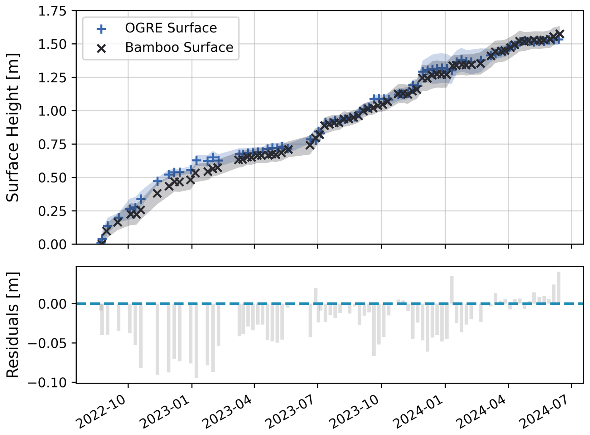
Figure 3 The comparison between the mean 24 h height estimates of the OGRE and the mean height estimates from a selection of the nearby 36 stakes within Bamboo Forest. Note that the H_r estimates for both the OGRE and the stakes have been flipped to show the increasing surface height, as opposed to the decreasing height between the fiducial and the surface. The shaded uncertainties are taken to be the 1σ values of the OGRE height estimates for a 24 h period and the 1σ values of the heights of the stakes, corrected to the same horizontal reference.

Overall, we observe a mean bias of $-\mathrm{2.7}\pm \mathrm{3.0}$ cm (n=76) between the averaged daily OGRE H_r and the 6-by-6-stake array, with a correlation coefficient of 0.998 (r²=0.996) (Fig. 3). Compared to the 6.0 cm variance found by Siegfried et al. (2017), an F test for equality of variances indicates that there is a significant large difference between the precisions ($p=\mathrm{1.4}\times {\mathrm{10}}^{-\mathrm{9}}$). We attribute the higher precision in this study to the centered spatial representativeness of the validation data set and perhaps a smoother reflecting surface. However, the OGRE-estimated surface is higher than the stake surface, especially in wintertime months, and this may be due to radio shadowing from surface features, a more difficult measurement environment due to snow build-up, or scouring at the base of the stakes affecting the manual stake measurements. Throughout the study, the heights of the OGREs were occasionally manually measured from the antenna ground plane to the snow surface; the mean bias was 2.5±3.1 cm (n=31), which is the same sign as the bias found by Siegfried et al. (2017). This indicates the OGREs overestimate H_r relative to the manual point measurements.

We also observe that the residuals are not uniform throughout the study, appearing higher in late fall and wintertime months. This seasonal effect appears to correspond to periods of higher uncertainty, indicative of a rougher surface, or perhaps the variability is partly due to scouring and pitting around the bamboo stakes. During the first year of the study, the temporal offsets between manual stake measurements and OGRE measurements were also the largest, potentially skewing the biases. These variations warrant a more robust investigation into the extent to which changing climatic and surface conditions influence reflectometry results. Nonetheless, we observe a better overall precision than previously published results from the cryosphere and a comparable bias relative to other studies.

3.3 Intercomparison of L1 and L2 frequencies in surface determination

An additional strength of the OGRE is its multi-constellation and multi-frequency tracking ability, which results in hundreds of successfully calculated H_r measurements for a 24 h period. It is important to analyze whether there is a statistically significant difference between L1 and L2 frequencies that arises due to different penetration depths or antenna phase center locations, which will influence how we consider these two signals when we aggregate our data.

Table 1 Pairwise biases between L1 and L2 frequencies, showing very low biases for intra-constellation differences in L1 and L2 frequency H_r estimates.

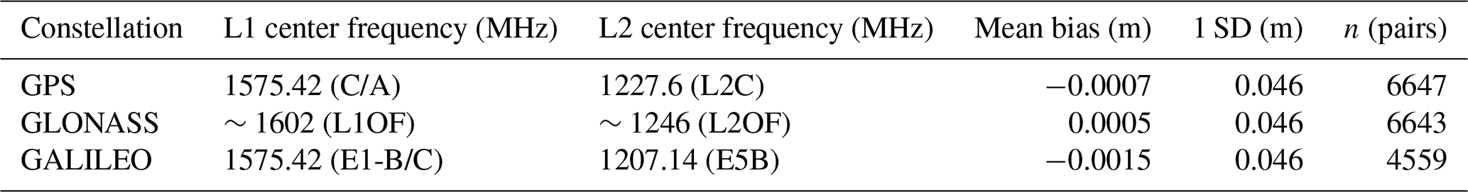
We identify any individual satellite arcs across all constellations where both L1 and L2 frequencies from the given satellite produce H_r estimates in our processing routine. We then compute the mean of the biases between all these pairwise points by constellation (Table 1). Across all aggregated data, we find no statistically significant evidence (p<0.01) that the biases differ from zero for any constellation. This suggests that the differences in frequency or antenna phase center location are not enough for a detectable difference in H_r measurements over sources of noise or processing errors. These biases are smaller than those reported in Larson and Small (2016) for GPS signals, perhaps due to improvements in L1 tracking or a smaller L1/L2 phase center difference in the antennas used in this study. These results allow us to further assess the precision of an individual H_r estimate by considering L1 and L2 H_r estimates together.

3.4 Individual H_r measurement precision

Section 3.3 demonstrated that we can consider H_r estimates from L1 and L2 together. As this study seeks to evaluate surface heterogeneities from H_r estimates, we first need to understand the precision of individual H_r estimates. In general, if we wished to assess the noise and precision of single H_r estimates corresponding to particular satellite arcs, we would conduct a repeatability test from one day to the next with an unchanging surface. However, while we consider a 24 h period of surface heights to be static, we cannot necessarily make the same assumption from one measurement period to the next. Given the large amount of data and the general agreement between L1 and L2 height estimates, we instead assess the variability in the mean surface for any period.

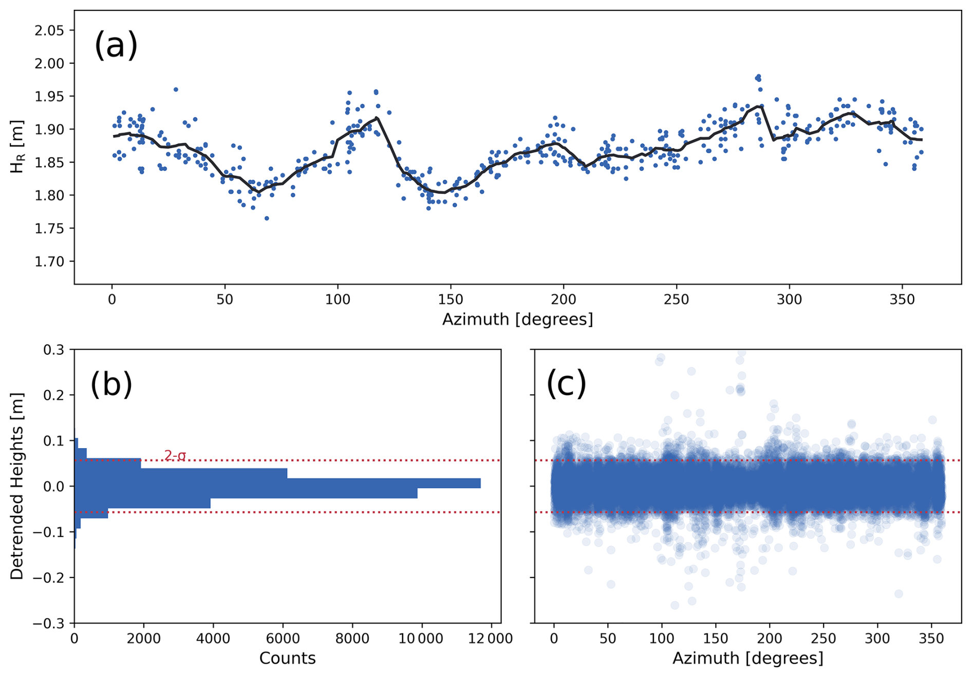
Figure 4 (a) Example 24 h period of H_r measurements from an OGRE with the mean surface determined by passing the data through a kernel filter tuned to encompass 10° azimuthal windows. (b, c) All detrended surface height H_r data points for the Bamboo Forest OGRE across all measurement periods are aggregated together and show an approximately normal distribution. The 1σ value (2.8 cm) is taken to be the precision value for any single H_r estimate.

In Fig. 4a, we see an example aggregate of H_r estimates for a 24 h period, plotted based on azimuthal location about the OGRE. These H_r estimates show a low-frequency signal when plotted azimuthally. As H_r estimates are semi-randomly sampled temporally, changes in atmospheric or surficial conditions throughout the 24 h window cannot contribute to this low-frequency signal, indicating the signal is more likely caused by surface topography variations. In the next section, we more definitively link this signal to surface features, but, in order to assess precision, here we remove this azimuthal trend in the data by applying a fixed-bandwidth Gaussian kernel smoother to find and subtract the azimuthally varying mean surface. Firstly, any H_r outliers (>3σ) are removed for a given 24 h data period. We then remove any days where there is a statistical temporal trend in the data (p<0.01), indicating that detectable accumulation occurred during the 24 h period. This occurred during 8 d throughout the study. The removal of outliers and temporal-trending days reduces the total number of H_r points from 39 480 to 35 340. Finally, we define a bandwidth window that encompasses 10° azimuthal chunks of the data in order to apply the filter to remove the low-frequency signal.

Aggregating all detrended measurement data yields a 1σ of 2.8 cm (n=35 340) (Fig. 4). This value represents the precision of any single H_r measurement and may still encompass errors from variable surface conditions throughout the study and processing errors. However, this value agrees with estimates made in past studies showing that individual satellite signals produce height estimates varying on the order of 2–3 cm (Larson and Small, 2016). Furthermore, Gutmann et al. (2012) estimates the formal error of the GNSS-IR method to be 2 cm, while Larson and Nievinski (2013) estimate this error to be 2.5 cm, which indicates these formal and processing errors largely constitute the estimate of this precision.

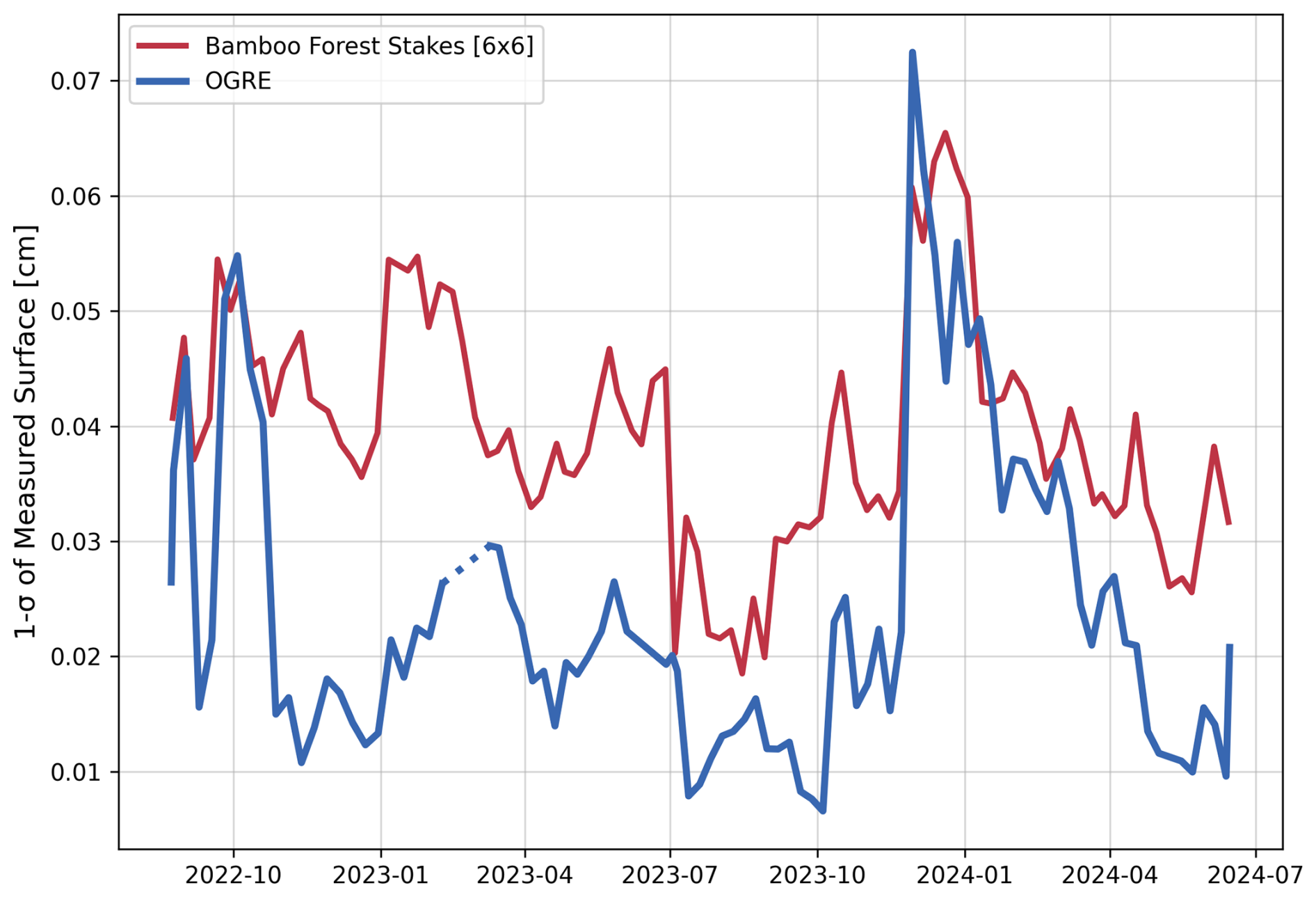
Figure 5 Bamboo Forest surface roughness (derived from 6-by-6 inner stakes) compared to OGRE surface roughness. Note that, between February 2023 and March 2023, the OGRE did not record any data, as it was temporarily removed from the field for a firmware upgrade.

4 Surface roughness measurement validation

4.1 A new technique for measuring surface roughness

We now evaluate the sensitivity of OGRE reflectometry-derived H_r estimates to surficial features such as sastrugi and dunes. For a given 24 h period, we first remove outliers as in Sect. 3.4. We then apply the same 10° fixed-bandwidth kernel filter to derive the underlying low-frequency signal, resampling the signal to 1° bins to ensure a uniform spatial sampling. Finally, we fit a sinusoid with a period of 1 per 360° to the data to remove the underlying surface slope, and we take the standard deviation of the detrended data. This value is taken as the OGRE-derived surface roughness. Similarly, for the Bamboo Forest data, we remove the plane of best fit from the subset of 36 stakes closest to the OGRE and take the standard deviation to represent the surface roughness, covering a spatial extent of 40 m by 40 m. Over the study period, we find that the OGRE-derived surface roughness correlates with the Bamboo Forest stakes (r=0.74, $p=\mathrm{1.5}\times {\mathrm{10}}^{-\mathrm{14}}$, n=76), again using a ±48 h search for comparisons (Fig. 5). During the final year of the study, a heightened surface roughness state is detected by both methods and the correlation is 0.89.

We also conducted this comparison for increasingly larger and smaller subsets of bamboo stakes, with monotonically decreasing correlation coefficients from 0.74 for the 36 stakes to 0.56 for the entire 121-stake network and a correlation of 0.51 for the inner 4 stakes. Across the range of OGRE antenna heights in this study, this comparison indicates that the technique is most sensitive to the surface 4–20 m radially from the OGRE location, aligning with our findings from the accumulation comparison. To test for the choice in the bandwidth window, we varied the window size from 5 to 40° and found that the two data sets still have moderate to high correlations, perhaps due to a multi-scale correlation in surface roughness, but with diminishing agreement as the filter over- or underfits the reflectometry data.

The 36 stakes, which are spaced at 8 m in a grid, act like a low-pass filter and are sensitive to surface features that have wavelengths close to or exceeding this spacing. Meanwhile, large-scale features with a wavelength greater than the distance of the total spatial extent (40 m in either direction) are removed when the plane of best fit is removed. For the OGREs, each H_r estimate is effectively a spatially averaged surface based on the Fresnel geometry; thus features with wavelengths smaller than these ellipse widths (2–4 m) will minimally bias the height estimates, although this sensitivity may vary based on the anisotropy of the roughness. The maximum wavelength sensitivity for this technique approximately corresponds to the diameter of the total circular footprint, or 50–70 m. As for sensitivity to the amplitude of these features, both techniques are precise at centimeter level; thus they are sensitive to centimeter- to meter-scale feature heights. At Summit, Albert and Hawley (2002) have shown that the characteristic wavelengths and amplitudes of prominent roughness features fall within the detectable range of both the OGREs and the Bamboo Forest, with 5–20 m wavelengths and 3–20 cm amplitudes. With OGRE-derived roughness, however, it is difficult to connect these undulations to physical locations given the spatial footprint characteristics, but we can nonetheless detect when features at these wavelengths and amplitudes change in spacing or scale.

Perhaps the largest source of error between the two roughness estimates is the spatial extent: while surface roughness can be correlated across spatial scales due to its fractal nature (e.g., Zuhr et al., 2021), the differences in footprint size between the OGRE and Bamboo Forest will lead to different measurements. We also made the assumption that no accumulation takes place during the 24 h measurement periods; however, this is not always the case, as eight periods had a statistically significant slope in H_r versus time (p<0.01) that indicated a sub-daily surface change rate of several centimeters per day, with the same sign as the week-over-week change surrounding that day. Furthermore, the standard deviation calculation is sensitive to outliers, and, while we remove measurement outliers greater than 3σ for any given survey for the stakes, error propagation and systematic errors could compound, especially on dates far from the automatic level survey conducted during June 2024. As previously discussed, the OGRE footprint shrinks throughout the 2-year study as the surface accumulates relative to the antenna, which leads to further mismatch between the two footprints. However, the results presented thus far provide a compelling demonstration that most of the azimuthal variability in H_r measurements is due to real, time-varying structural features in the sensing domain.

We further validate the extent and properties of the sensing area by examining the 10 cm resolution TLS surface scan (Fig. 2a) in the Bamboo Forest from 16 June 2024, where we found only a moderate relationship (r=0.36) between OGRE H_r estimates mapped to the TLS surface, with the slopes removed. By imposing Fresnel zones calculated from 0.1° elevation angle spacing from 5 to 25° on the TLS surface, we can reconstruct the GNSS-IR footprint to extract mean surface values. A discussion on the potential sources of error that led to the lower agreement between the data sets is provided in Appendix B.

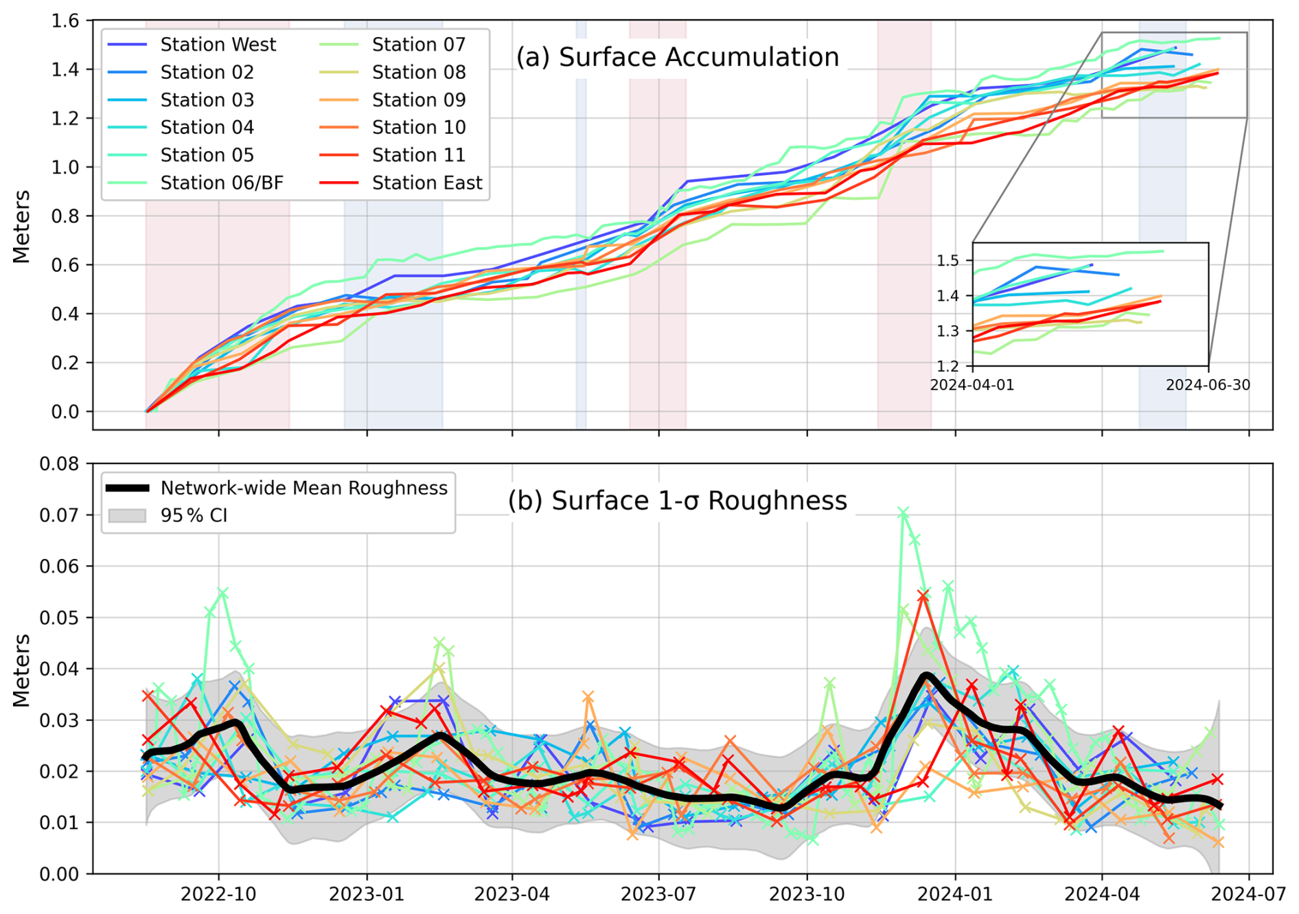
Figure 6 (a) Accumulation through time of all 12 OGRE stations, with periods of elevated accumulation or low/negative accumulation highlighted in light red and blue, respectively. The OGRE station time series are colored from blue to red to indicate location from west to east. (b) 1σ (roughness) values through time of all stations, with the mean network-wide value indicated by the thicker black curve.

5 Results and discussion

5.1 Network-wide spatial and temporal patterns in accumulation

Incorporating data from all 12 stations, we show accumulation and surface roughness based on 24 h intervals of recorded data at each station throughout the study period (Fig. 6). From August until November 2022, accumulation rates were nearly 10 standard deviations higher than the overall mean rates for most stations. Notably, the annual accumulation rate from September 2022 to September 2023 is nearly 95 cm yr⁻¹ at the Bamboo Forest OGRE, which is much higher than rates previously found by Dibb and Fahnestock (2004) (64–65 cm yr⁻¹) and in the upper 95th percentile of the 71±11 cm yr⁻¹ mean rate found over 10 years of Bamboo Forest data (Castellani et al., 2015). While much of Greenland experienced melt due to several atmospheric river events during September 2022 (https://nsidc.org/ice-sheets-today/analyses/record-september-greenland-ice-sheet-melt, last access: 20 August 2024), this precipitation fell as snow at Summit Station and contributed to the anomalously high rates of accumulation over the period.

In 2023, several stations again experienced local accumulation rates much higher than their averages in June and July and from mid-October to December, while 2024 featured no such enhanced accumulation prior to the end of the study. Meanwhile, near-zero or negative accumulation rates were observed for a number of stations between mid-December 2022 and March 2023 and from mid-April to June 2024. Temporal patterns of accumulation suggest that the observations made by Dibb and Fahnestock (2004), Howat (2022), and Castellani et al. (2015) still hold true: there is a marked increase in stake height change for all stations during the late summer and early fall when precipitation is generally high but firn compaction rates decrease from summertime highs and a lower period of accumulation (or negative accumulation) in the late winter and spring, which is perhaps driven by enhanced negative processes described in Eq. (1). However, the Bamboo Forest OGRE exhibited a mean annual rate of 77.8±10 cm yr⁻¹, which trends higher than previously reported annual rates for this location. The Bamboo Forest OGRE recorded an especially high rate of accumulation in the winter of 2023 relative to the other stations, and we posit that a combination of winds and its proximity to drift-inducing structures may have led to the emphasized surface height increase.

From Station 11 (closest to the divide) across-slope to Station West, the slope is −0.067° and spans 34.7 km with a vertical drop of 43.7 m, and these stations exhibit an across-slope difference in accumulation over the 2-year period, which is visible in the inset in Fig. 6. We find the mean rate of accumulation over the study period by averaging a sliding window of 365 d; Station 11 has a mean accumulation rate of 70.9±4.2 cm yr⁻¹, and Station West exhibited a mean rate of 77.4±4.7 cm yr⁻¹. Because the uncertainties for each station are correlated, we use a t-test of the slopes of a linear regression fit over the entire period of data to confirm statistical significance in the accumulation rates between these two stations (p=0.04). Furthermore, we find that MERRA-2 precipitation rates vary between these two locations by a similar amount, 79.4±4.9 and 85.9±5.1 cm yr⁻¹, using an assumed density of 300 kg m⁻³, a common value for surface snow at Summit, to convert liquid volume to estimated snow thickness (Montgomery et al., 2018). Here, the difference is 6.5 cm yr⁻¹, which mirrors the 6.5 cm yr⁻¹ difference in the OGREs. This indicates that both MERRA-2 and the OGREs are sensitive to the dominant variations in moisture that originate from the west and southwest in this region (Bolzan and Strobel, 1994).

The across-network spatial variability in accumulation takes two factors into account: semi-random localized accumulation within the spatial footprint of each OGRE and a small along-slope increase in precipitation from the divide to the west. Since each station often logs on independent days of the month compared to the others, we interpolated H_r measurements to daily measurements, removed the station-specific accumulation trend, and calculated the standard deviation for each day between stations to find the inter-station variability in accumulation driven by localized differences in Eq. (1). The mean standard deviation between the detrended data is 2.6 cm, suggesting that, on monthly scales and at 10 km spacing within our study area, spatial variability in accumulation is small between stations. However, we note that, from November 2023 to January 2024, the mean standard deviation of the detrended network peaks at 4.0 cm, which is the same period of heightened local variability for many stations (Fig. 6).

5.2 Network-wide temporal patterns in surface roughness

There are three periods when several stations or a majority of stations show heightened roughness above the 2.8 cm individual precision threshold: in September and October 2022, February and March 2023, and December 2023 through February 2024. These periods indicate a seasonal pattern of heightened roughness that corresponds to either higher snowfall, which can be heterogeneously distributed or eroded, or periods where winds play a dominant part in snow removal with negative or little accumulation. Interestingly, no heightened roughness is detected in the summertime months despite instances of high accumulation or negative accumulation that mirror similar events in winter months. The drivers of accumulation in Eq. (1), including wind, latent heat flux, and compaction, all vary seasonally (Castellani et al., 2015), and, while they only account for a small percentage of the total accumulation in the Summit region (e.g., Lenaerts et al., 2012), these factors may play a larger role in driving the seasonality in roughness observed here.

The agreement between most stations indicates that the conditions of surface roughness across the network are largely the same; small variations in roughness amplitudes could cause some of the observed differences, although we would expect amplitude to be largely correlated across this region. Albert and Hawley (2002) noted that the wavelength between snow features showed little seasonal pattern, and perhaps spatial differences in wavelength may also partially explain the variation in roughness measurements between stations.

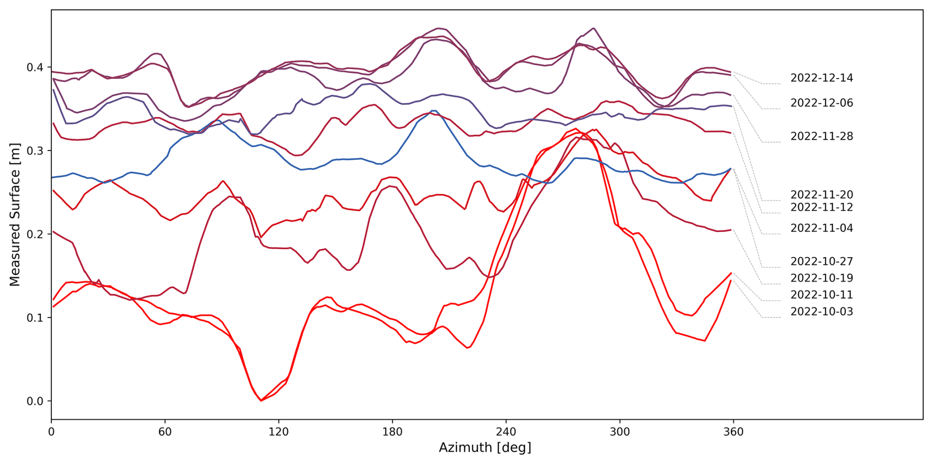
Figure 7 Several GNSS-IR-derived surfaces from the Bamboo Forest OGRE plotted azimuthally, showing patterns of accumulation between October and December 2022. Color is based on the correlation of each data period to the first profile on 3 October 2022, with red indicating the most correlation and blue indicating the least correlation.

5.3 Local spatial and temporal patterns in surface roughness

Figure 7 shows several OGRE-derived H_r profile estimates, plotted based on azimuthal direction. For ease of viewing, we run a local polynomial filter over each data series to provide a continuous line for easy viewing while masking individual H_r estimates. We also colored each time series based on its correlation to the first (3 October 2022) measurement, with red indicating a correlation coefficient of 1 and blue indicating the lowest correlation coefficient value. Here, the surface starts with a heightened roughness state, with a large peak spanning the western quadrant of the instrument. Through time, the surface evolves due to positive or negative accumulation processes (Eq. 1). We prescribe a physical explanation of the surface evolution: the surface generally increases but not uniformly. As the troughs around the initial 30 cm October feature fill in, the peak remains at the same elevation or even erodes until it is completely buried. This pattern matches that described by Filhol and Sturm (2015), whereby wind-affected snow will show preferential erosion or deposition based on exposure: wind-sheltered regions fill in first, while wind-exposed features remain exposed to erosion.

Furthermore, we note that the correlation between each subsequent time series and the first measurement is not monotonically decreasing. This may suggest that well-sintered features may be preserved in the snowpack after an accumulation event and become re-excavated or play some part in the overlying snow topography (Zuhr et al., 2021). Ultimately, care must be taken in interpreting these daily time series given the geometric constraints discussed in Sect. 2.4. For example, the 30 cm “peak” on 3 October is a shallow mound that spans over a 100° field of view from the perspective of the instrument. As each reflector height estimate is composed of inputs from a variety of satellite elevation angles and therefore varying Fresnel zone size and location, these apparent features may dampen or spatially average any true physical feature or preferentially emphasize raised surfaces due to radio shadowing (Bourlier et al., 2006).

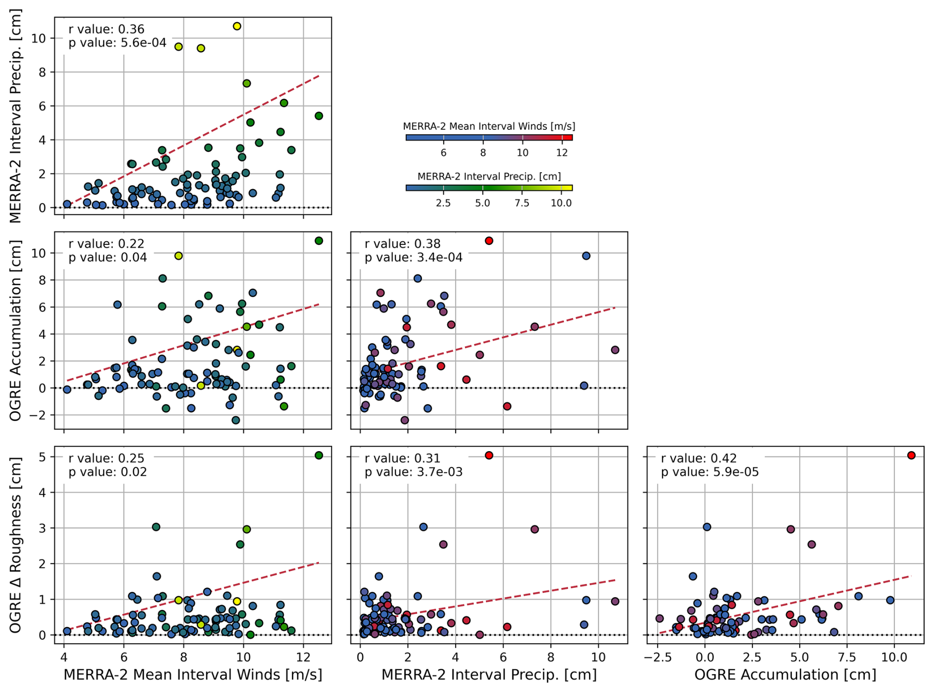
Figure 8 Intercomparison between weekly Bamboo Forest OGRE accumulation and roughness change data with MERRA-2 winds and precipitation.

5.4 Surface roughness and accumulation connection to meteorology

For a process-level understanding of the drivers of accumulation and surface roughness expressions observed by GNSS-IR and illustrated in the previous section, we compare OGRE data to MERRA-2 precipitation and winds (Fig. 8). We specifically examine the data from the Bamboo Forest OGRE, given the weekly sampling rate. For each period between samples, we derive interval precipitation by calculating the cumulative precipitation scaled to a snow thickness using an assumed density of 300 kg m⁻³, and we derive interval winds by calculating the mean wind speeds during each period. We then compare these MERRA-2-derived variables to accumulation (ΔH_r) from the OGRE, along with surface roughness change, Δσ. This comparison is similar to those made by Picard et al. (2019) in Antarctica and Zuhr et al. (2021) in Greenland.

MERRA-2 precipitation and MERRA-2 winds have a low to moderate correlation and high statistical significance, which may be explained by observations by Pettersen et al. (2018) that the ice and mixed-phase clouds that bring moisture to the Summit originate from strong southerly storms that exceed average yearly wind speeds. Meanwhile, OGRE accumulation and MERRA-2 winds show a lower correlation and marginal statistical significance; this may be due in part to negative OGRE accumulations that are a result of more erodible soft-snow conditions in winds (Filhol and Sturm, 2015). When we compare net OGRE accumulation with winds or remove the negative accumulation values, we increase statistical significance and the correlation value to 0.27, but we lack the necessary data to investigate the environmental factors that lead to positive or negative accumulation during high winds.

Unlike in Picard et al. (2019) or Zuhr et al. (2021), we correlate the surface roughness change from one period to the next as opposed to the measured surface roughness because of the interval of our measurements. For example, a surface may maintain a rough state for several days if no new snow or winds occur, whereas the change in surface roughness state may be more readily explained physically by the presence or lack of precipitation and winds. The low correlation but statistical significance between surface roughness change and winds suggests that wind speed can play a role in surface roughness, but other factors such as the hardness of the existing snow must be considered simultaneously, alongside cumulative precipitation and surface accumulation. These variables have low to moderate correlations when compared to surface roughness change, with positive precipitation or accumulation perhaps providing the necessary material to modify the roughness state either by surface smoothing or by irregular deposition. Overall, the interpretation that higher winds correlate with increases in surface roughness is supported by the observed behavior of wind-driven surface roughness observed at the South Pole (McConnell et al., 1997), but our study only indicates whether winds directly lead to magnitude change in surface roughness and not whether the surface became more or less rough compared to its prior state.

Finally, OGRE accumulation and cumulative precipitation show a moderate correlation with high statistical significance. The relationship between precipitation and OGRE accumulation is skewed downwards from a 1:1 relationship, suggesting that other factors, such as sublimation, compaction, and variability in surface density may need to be included in a more comprehensive analysis, especially as MERRA-2 precipitation alone cannot explain negative accumulation values and the smaller OGRE spatial representativeness cannot exactly capture the MERRA-2 interpolated estimates.

6 Conclusions

We have expanded the scope of the GNSS-IR technique in the cryosphere by validating GNSS-IR-derived measurements, examining the spatial extent and temporal reliability of this technique, and assessing its sensitivity to local surface heterogeneities. Here, averaged 24 h periods of GNSS-IR estimates are biased by −2.7 cm in low-angle dry snow and are precise to 3.0 cm relative to manual measurements. This precision is better than any previously reported in the literature for snowy environments, and this is partly due to a comparison to a more spatially representative validation data set. However, the biases between the GNSS-IR heights and the validation data set warrant further investigation as to the slight differences in wintertime and summertime. It is now common for receivers to track both the L1 and L2 signals of multiple constellations, and we also show that there are no biases between the two signal types, allowing us to effectively double the size of our data set.

We also assessed the spatial extent of this surface-sensing technique. While we model the moving ground reflection locations of each satellite signal arc and find them to span from 4–35 m radially for a 2 m antenna, we found that the derived surface height estimates across the 1–2 m antenna height range are most sensitive to the inner 4–20 m about the instrument, based on the best correlation with a subset of snow stakes. The characteristics of this sensitivity have several implications for the sensing footprint. Firstly, this technique can average over a larger area than point measurements and remove high-frequency surface noise, providing a more spatially representative measurement for daily or sub-daily surface accumulation. Secondly, this technique provides additional context for understanding the circumferential spatial heterogeneity that we estimate, limiting our window of sensitivity to centimeter- to meter-sized features that populate this footprint. We find that these surface roughness values of the OGRE share the same magnitude and pattern of roughness variations with a 36-stake network grid spaced at 8 m (r=0.74). Temporal sampling offsets, differing spatial footprints, and measurement error from the validation data set likely account for disagreements in roughness magnitude and timing between the two data sets, but they both show fidelity in detecting increased wintertime roughness states.

We then assessed accumulation and surface roughness values derived from a network of 12 low-cost GNSS stations in the interior dry-snow zone of Greenland for spatial and temporal patterns compared to historical data. Accumulation patterns are largely consistent with historically observed increases in late summer and early fall enhanced height, along with decreased rates in the springtime. This network also detected a centimeter-level variation in accumulation at yearly scales between the easternmost and westernmost stations, which we interpret as a cross-slope variation in accumulation consistent with expected higher downslope accumulation rates. Meanwhile, surface roughness trends exhibited several wintertime periods of increased roughness, and it was during these periods that the greatest spatial variability (±4.0 cm) was observed in accumulation between stations. Furthermore, these results suggested that both erosional feature formation and depositional heterogeneities can drive an increased roughness at centimeter to meter scales in the Summit vicinity.

For process studies, we demonstrated the utility of GNSS-IR measurements for better understanding snowpack stratigraphy and the preservation or erosion of snow layers through time. We connected height and roughness measurements with wind and precipitation from MERRA-2 to show that these synoptic variables contribute to the accumulation and structure of snow in the Summit vicinity, but we also highlight that there must be other processes or variables, such as sintering time, that may have a more dominant role in the preservation or erosion of snowpack. This exercise highlights the GNSS-IR technique as an easily executable, adaptable method that can shed light on processes that have previously been difficult to measure in the field, such as wind scour and firn compaction. The ease with which these GNSS instruments can be configured to take daily measurements further accentuates the ability of this technique to illuminate short-timescale processes and trends.

Ultimately, these results are local to a relatively flat, accumulating 30 km region in the vicinity of the Greenland Ice Sheet summit, but the methods presented here show promise throughout the cryosphere. Low-cost GNSS devices, such as those presented in this paper, are more easily deployable in large quantities due to their smaller size and weight, cost, and energy efficiency, all while providing high-quality results and requiring no special configuration other than an elevated antenna. The reliability and resolution of the GNSS-IR technique is demonstrated to be sensitive to low accumulation signals, while we also show for the first time that the variability in individual H_r estimates is due in large part to surface roughness. These measurements can be combined to better assess ice core stratigraphy, measure turbulent heat flux in real time, and detect daily changes driven by precipitation, compaction, wind, and sublimation or serve as ground validation measurements for a variety of remotely sensed variables.

Appendix A: Further discussion on ground footprint of GNSS-IR

Nievinski and Larson (2014) show that, for a 2 m antenna height, there is an uneven weighting for the sensing footprint of reflectometry: the peak region of importance lies somewhere between 13 and 15 m from the instrument (corresponding to about a 10° satellite elevation angle), with regions closer to the antenna rapidly losing importance and regions farther than the peak gradually decreasing in importance. This spatial pattern arises for several reasons. At low satellite elevation angles, corresponding to a reflection farther from the instrument, the interferometric SNR pattern is often less noisy than the nearby portion of the signal (Fig. A1). This is further complicated by the ability of the Lomb–Scargle to determine the peak frequency and perhaps by the integer-binning of SNR readings by the receiver, which is a characteristic of the low-cost chip in the OGRE instruments.

Figure A1 Example SNR data from a single rising satellite arc from an OGRE on 18 August 2023, showing the characteristic integer-binning and degraded interferometric quality at higher elevation angles.

Nonetheless, this footprint interpretation is somewhat substantiated by the main text, as the 13–15 m dominant region falls within the 4–20 m zone identified as the most important region. However, our comparisons with both the TLS surface data and correlations to individual bamboo stakes show that nearby surfaces to the instrument are in fact more represented by the GNSS-IR solutions.

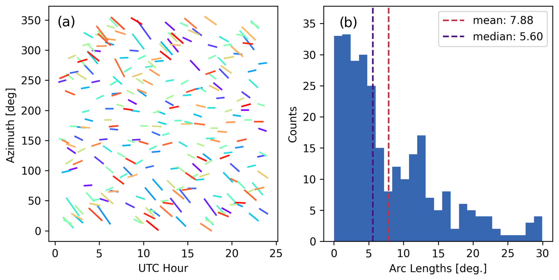
Figure A2 (a) Sample 24 h period of satellite azimuth projections, with each satellite represented by a different line, showing that every satellite has some azimuthal variation as it rises or sets, relative to the OGRE. (b) The mean arc is 7.88°, and the maximum is 29.95°. Across the entire study period, the mean arc is 8° and the maximum arc is 40°. In this study, we take the mean azimuthal value for each arc to represent the azimuthal location of that satellite arc.

A second point of note is that each H_r footprint corresponding to each arc is not necessarily perfectly radial to the instrument, as illustrated in Fig. 2. Each satellite arc contains an azimuthal component throughout the sky: for each 24 h period at an OGRE station at Summit, we measured the azimuthal angular distances, projected to the horizontal horizon plane, that the observed satellites travel as they rise or set through the critical elevation angle range of 5 to 25°. The mean azimuthal travel from all data is 8°, and the maximum azimuthal travel is 40° (Fig. A2). Consequently, there will be some azimuthal error in positioning singular reflector heights, which in turn will induce an error on estimating averages in particular quadrants or applying a fixed-bandwidth Gaussian kernel filtering technique. Furthermore, there is an azimuthal dependence for the length of the azimuthal arc; satellites to the north tend to move a greater horizontal distance across the sky than those to the south. This complicates any attempt to specifically pinpoint the location of an H_r estimate, and care must be exercised when attempting to directly compare an H_r estimate to a specifically located measurement such as at an individual snow stake.

Appendix B: TLS comparison and discussion

On 16 June 2024, we used a TLS to create a 10 cm resolution DEM of the Bamboo Forest surface. The OGRE concurrently recorded 24 h of data during this period. For each H_r estimate, defined by its azimuthal location, we sample the TLS surface based on the centroid of the evolving ellipse defined by the first Fresnel zone (FFZ) as it migrates closer to the OGRE and shrinks in size. Figure 2 demonstrates this geometry, which is driven by the satellite elevation angle. The azimuthal TLS height estimates are aggregated to create the TLS surface topography estimate for comparison to the OGRE surface (Fig. B1). A sample of TLS-derived surfaces for the annular distances defined by the 5–25° range is shown from light to dark gray. These FFZ annuli are averaged together to create the overall TLS-derived surface estimate, which we believe to be a good sampling approximation of the FFZ geometry.

Figure B1 From the 16 June 2024 TLS survey of the Bamboo Forest, we compare the OGRE height estimates to the TLS surface. The TLS surface is the composite of the sampled surfaces corresponding to the reflection points of simulated GNSS-IR reflected signals from R=5° (light gray) to R=25° (black).

The two surfaces are adjusted so that their mean value is centered at zero, yet the variance in the residuals between the OGRE and the TLS surfaces is higher than if we simply compared the OGRE surface to a planar surface. This low agreement could be attributed to a number of factors, including errors from the footprint positioning assumptions discussed in the previous section, errors from a slightly tilted antenna, and a slight evolution of the snow surface during the 24 h OGRE data period. Furthermore, this comparison averages across the full radial distance defined by the 5–25° elevation angles (per the FFZ pattern), but the GNSS-IR surface may be more sensitive to certain regions, leading to uneven weighting. For instance, the example SNR OGRE data show a cleaner sinusoid at low satellite elevation angles and therefore may be more heavily weighted towards these angles in the frequency estimation; thus the corresponding surface further from the antenna is more important. Conversely, the main text argues that the GNSS-IR-derived measurements correlate better with point measurements near the OGRE, which would favor the data from the 15–25° elevation bands.

To investigate these differences, we remove the area-wide surface slope from both the OGRE and TLS data and compare the resultant surface estimates from both techniques (shown in the second plot in Fig. B1). Here, the surfaces are not more correlated than previously (r=0.36); however, they visually share peaks and troughs, albeit somewhat offset, especially outside the 150–200° range. The non-linear phase shift may be indicative of the effect demonstrated in Fig. A2, where more northerly H_r estimates are in fact biased in their locations based on the arcing path of each satellite. The similarity in magnitude of the peaks could explain how the OGRE, while showing low agreement with TLS surface measurements, is still sensitive to the detrended surface roughness measurements described in this text.