the Creative Commons Attribution 4.0 License.
the Creative Commons Attribution 4.0 License.
 | 29 Feb 2024
Melt pond fractions on Arctic summer sea ice retrieved from Sentinel-3 satellite data with a constrained physical forward model
Larysa Istomina
Marcel Nicolaus
Ran Tao
Aleksey Malinka
Eleonora Zege
Gunnar Spreen
The presence of melt ponds on Arctic summer sea ice significantly alters its albedo and thereby the surface energy budget and mass balance. Large-scale observations of melt pond coverage and sea ice albedo are crucial to investigate the role of sea ice for Arctic amplification and its representation in global climate models. We present the new Melt Pond Detection 2 (MPD2) algorithm, which retrieves melt pond, sea ice, and open-ocean fractions as well as surface albedo from Sentinel-3 visible and near-infrared reflectances. In contrast to most other algorithms, our method uses neither fixed values for the spectral albedo of the surface constituents nor an artificial neural network. Instead, it aims for a fully physical representation of the reflective properties of the surface constituents based on their optical characteristics. The state vector X, containing the optical properties of melt ponds and sea ice along with the area fractions of melt ponds and open ocean, is optimized in an iterative procedure to match the measured reflectances and describe the surface state. A major problem in unmixing a compound pixel is that a mixture of half open water and half bright ice cannot be distinguished from a homogeneous pixel of darker ice. In order to overcome this, we suggest constraining the retrieval with a priori information. Initial values and constraint of the surface fractions are derived with an empirical retrieval which uses the same spectral reflectances as implemented in the physical retrieval.
The snow grain size and optical thickness change with time, and thus the ice surface albedo changes throughout the season. Therefore, field observations of spectral albedo are used to develop a parameterization of the sea ice optical properties as a function of the temperature history of the sea ice. With these a priori data, the iterative optimization is initialized and constrained, resulting in a retrieval uncertainty of below 8 % for melt pond and 9 % for open-ocean fractions compared to the reference dataset. As reference data for evaluation, a 10 m resolution product of melt pond and open-ocean fraction from Sentinel-2 optical imagery is used.
- Article
(15293 KB) - Full-text XML
- BibTeX
- EndNote


In the central Arctic, summer starts, depending on latitude, in May and lasts until late August or early September. This period is defined by the presence of solar shortwave radiation rapidly warming the air and sea ice surface. The heat uptake by the ocean is limited by the sea ice cover, which acts as a protective shield against the incoming solar radiation because of its high albedo. Thick, white ice or even snow-covered ice reflects more than 70 % of the incoming radiation back into the atmosphere (Malinka et al., 2018; Light et al., 2022), while the darker, open ocean would absorb 90 % of the solar energy if it was not protected by sea ice (Pohl et al., 2020). Thus, changes in sea ice extent, thickness, or albedo have a strong impact on the Arctic energy budget (Fetterer and Untersteiner, 1998; Perovich et al., 2002; Nicolaus et al., 2012). Melt ponds, which form on the Arctic sea ice surface once the melting point is exceeded, drastically lower the surface albedo (Eicken et al., 2004; Istomina et al., 2015a; Light et al., 2022) and lead to increased absorption of solar radiation in the sea ice and upper ocean (Perovich et al., 2003). This in turn accelerates the sea ice melt and is known as the sea ice–albedo feedback mechanism (Curry et al., 1995; Perovich et al., 2008; Wendisch et al., 2023). Due to this feedback mechanism, some studies find that melt ponds could be used to predict the seasonal Arctic sea ice extent minimum in September (Schröder et al., 2014; Liu et al., 2015), which has been dramatically declining in the past decades (Stroeve et al., 2012b, a; Screen, 2021). Additionally, melt ponds strongly impact the Arctic ecosystem because the increased amount of available photosynthetically active radiation in and beneath the ice enhances primary production (Frey et al., 2011; Light et al., 2015; Katlein et al., 2019; Nicolaus et al., 2022).
Field observations help us understand the formation processes and seasonal evolution of melt ponds (Yackel et al., 2000; Perovich et al., 2002; Eicken et al., 2004; Polashenski et al., 2012; Webster et al., 2022). However, these studies also show high temporal and spatial variability of melt pond formation and coverage, especially on undeformed first-year ice (Scharien and Yackel, 2005). This variability is challenging but necessary to represent in global climate models (Flocco and Feltham, 2007; Dorn et al., 2018; Hunke et al., 2013; Zhang et al., 2018) to realistically simulate the albedo and mass balance of Arctic sea ice. Therefore it is essential to analyze the large-scale distribution and evolution of melt ponds and thereby quantify the importance of sea ice in terms of Arctic amplification and its impact on the global climate system (Serreze et al., 2009; Wendisch et al., 2023). For this purpose, satellite observations are the only suitable measurements. They can cover the entire Arctic on a regular basis at coarser resolutions of 500 m to 1.2 km daily. The first pan-Arctic melt pond fraction product was developed by Tschudi et al. (2008) using MODIS (Moderate Resolution Imaging Spectroradiometer) spectral surfaces reflectances in the optical range. They use fixed reflectance values for the surface type components though, which does not account for the high variability of sea ice and melt pond optical properties; this can lead to misclassification and larger uncertainties. Approaches generating pan-Arctic melt pond fraction datasets mostly involve artificial neural networks (Rösel et al., 2012; Ding et al., 2020; Lee et al., 2020; Feng et al., 2022; Peng et al., 2022). However, there are discrepancies of more than 10 % between melt pond fraction products (Lee et al., 2020), and the artificial character of the retrievals impedes the analysis and understanding of the physical reasons. Zege et al. (2015) have developed a physical retrieval, which is based on field observations of melt pond and sea ice spectra (Polashenski et al., 2012; Istomina et al., 2013) as well as the representation of the bidirectional reflectance of the surface as a function of its physical properties as suggested in Malinka et al. (2016, 2018). This approach enables a better assessment of retrieval performance (Istomina et al., 2015a, b) and adjustments with regard to a changing Arctic without the need for new training data.
We present a new algorithm, called MPD2, that builds on the implementation of the physical MPD1 retrieval by Zege et al. (2015) and Istomina et al. (2015a, b). While MPD1 was developed for the distinction between two surface types, sea ice and melt ponds only, we add a third (open ocean) surface type class to avoid a systematic overestimation of melt ponds. Knowledge gained from field observations of summer sea ice and melt ponds is used to initialize and constrain the retrieval and thereby afford the additional free parameter. A parameterization is developed from in situ spectral albedo measurements to estimate sea ice properties as a function of the air temperatures the sea ice has undergone. This is motivated by the temporal sea ice albedo change, which also depends on the temperature (changes in snow grain size and optical thickness). As we are retrieving sub-satellite-pixel surface fractions, such unaccounted for albedo changes in the sea ice–snow surface type would negatively impact the retrieval uncertainty. Additionally, we have developed an empirical retrieval of the three surface types, which serves as an initial step to provide constrained surface fraction values as a starting guess for the physical melt pond retrieval. This initial empirical retrieval is based on the difference between the spectral signals of the surface types (Tschudi et al., 2008; Rösel et al., 2012; Istomina et al., 2015a; Light et al., 2022). The MPD2 algorithm is implemented for the Sentinel-3 satellite sensors OLCI (Ocean and Land Color Instrument) and SLSTR (Sea and Land Surface Temperature Radiometer) using top-of-the-atmosphere (TOA) measured reflectances in the visible and near-infrared range at a spatial resolution of 1.2 km. Comparisons are drawn to the MPD1 algorithm (Istomina et al., 2023) and to a 10 m resolution melt pond and open-ocean fraction product derived from Sentinel-2 optical data (Niehaus et al., 2023). The focus of this study about the new MPD2 retrieval is the melt pond fraction product, which is also mainly evaluated here. However, along with melt pond fraction, the open-ocean fraction and surface albedo are retrieved.
The central algorithm presented in this work is based on optical data acquired by the Sentinel-3 satellites. For the processing, in addition, the low-resolution sea ice drift product of the EUMETSAT (European Organization for the Exploitation of Meteorological Satellites) Ocean and Sea Ice Satellite Application Facility (OSI SAF, https://www.osi-saf.org, last access: 1 October 2023) and the reanalysis 2 m air temperature product by ERA5 are used. For the development, in situ spectral albedo measurements are investigated. The evaluation of the presented algorithm is performed based on the melt pond fraction product derived from optical Sentinel-2 satellite data.
2.1 Sentinel-3 top-of-the-atmosphere reflectances
The retrieval algorithm uses top-of-the-atmosphere (TOA) measurements supplied by the EU Copernicus Sentinel-3A and Sentinel-3B satellites operated by the European Space Agency (ESA) and European Organisation for the Exploitation of Meteorological Satellites (EUMETSAT). The two satellites orbit the Earth, phased by 180°, at an altitude of approximately 815 km in a polar, sun-synchronous orbit since February 2016 and April 2018, respectively. With a swath width of 1270 km and a short revisit time, they cover the full Arctic, north of 67°, every day. However, optical observations are compromised by prevalent cloud contamination typical for the Arctic summer. Each of the two satellites carries multiple instruments, two of which are used in this work: the Ocean and Land Color Instrument (OLCI) and the Sea and Land Surface Temperature Radiometer (SLSTR). The OLCI measures the Earth's reflectance in 21 spectral bands in the visible and near-infrared (NIR) range (400–1020 nm) with a spatial resolution of 1.2 km in reduced-resolution mode and 300 m in full-resolution mode. In this study we use the reduced-resolution data in favor of computing time and because the complications of sub-pixel surface type features apply to both resolutions. The SLSTR measures TOA radiances and brightness temperatures in nine spectral bands in a range from 554 nm to 12 µm with a spatial resolution of 500–1 km. In the Level-1 products, the data are provided as geolocated measurements for both instruments; for OLCI the solar and observation angles are additionally provided.
2.2 OSI SAF drift product
For the tracking of the sea ice motion, the OSI-405 low-resolution sea ice drift product by EUMETSAT OSI SAF (OSI SAF, 2010) is used. It provides sea ice motion vector fields for a nominal time span of 48 h merging single-sensor drift vectors derived from various satellite sensors with an optimal interpolation scheme. The drift data are provided with an uncertainty estimate which ranges from 4 to 8 km. The product is a near-real-time product that is available daily since 2019 and with a grid spacing of 62.5 km, projected to the NSIDC polar stereographic grid.
2.3 ERA5 temperature
Along the drift track of ice parcels determined with the OSI SAF drift data, we use the 2 m air temperature provided by the ECMWF fifth-generation reanalysis ERA5 (Hersbach et al., 2020) to calculate a temperature index as described in Sect. 4.2. The data are downloaded from the ERA5 web page (https://cds.climate.copernicus.eu/cdsapp#!/dataset/reanalysis-era5-single-levels, last access: 30 September 2023) with a spatial resolution of 0.25° and a temporal resolution of 6 h.
2.4 In situ albedo observations of radiation stations
In situ observations of spectral albedo from various measurement campaigns (TARA campaign 2007, Nicolaus and Gerland, 2022; PS106-ARK31/1 expedition 2017, AlertMAPLI18 campaign 2018, and MOSAiC campaign 2019–2020, Nicolaus et al., 2022) are used in this work to investigate the relation between surface properties and the air temperatures. The datasets were obtained by the use of autonomous platforms installed on drifting sea ice. These platforms comprised two RAMSES spectral radiometers with a spectral resolution interpolated to 1 nm, covering wavelengths from 320 to 950 nm. They were mounted 1 m above the sea ice surface, measuring the incoming solar irradiance and upward-reflected solar irradiance. From these measurements spectral albedo is obtained and provided. More details on the measurement setup and instruments can be found in Nicolaus et al. (2010).
2.5 Sentinel-2 melt pond fraction
For the development and evaluation of the MPD2 algorithm, 10 m spatial resolution melt pond fraction data derived from Sentinel-2 satellite Level-1C optical imagery (Niehaus et al., 2023) are used. The dataset provides melt pond fraction and open-ocean maps up to latitudes of 82.3°, covering areas of 1000 to 10 000 km2 each (Niehaus and Spreen, 2022). The provided Sentinel-2 scenes are filtered by the availability of reasonable, cloud-free Sentinel-3 data within a time difference of less than 1 h, which results in 33 remaining scenes. To enable a quantitative comparison, the data from Sentinel-2 are drift-corrected to match the Sentinel-3 product by using the OSI SAF drift product described in Sect. 2.2.
The Melt Pond Detection 2 (MPD2) algorithm builds on the Melt Pond Detection 1 (MPD1) algorithm which was developed by Zege et al. (2015) to retrieve pan-Arctic melt pond fraction and surface albedo from optical satellite data. Initially, the algorithm was designed for application to data from the MERIS (MEdium Resolution Imaging Spectrometer) sensor on ENVISAT (Environmental Satellite) which operated from 2012 to 2022. The adaption for the application to the data acquired by the Sentinel-3 satellites is described in Istomina et al. (2023). In contrast to most other pan-Arctic retrievals, e.g., by Rösel et al. (2012), Ding et al. (2020), Lee et al. (2020), Feng et al. (2022), and Peng et al. (2022), the MPD algorithm is not based on the implementation of artificial neural networks but uses a radiative transfer model representing the reflective properties of melt ponds and white ice based on their physical characteristics. Herein, the white ice category comprises various types of sea ice surface combined due to their high albedo and white appearance. This includes bare sea ice with a thin but highly scattering surface layer on top, which is formed after meltwater has drained (Tschudi et al., 2008; Malinka et al., 2016), as well as snow in its different melting stages. These surfaces differ by their grain size, optical thickness, and other properties which, however, are all accounted for in the same metrics by Zege et al. (2015) so that sea ice and white ice are used synonymously in the following. The bidirectional reflectance distribution function (BRDF) (Nicodemus et al., 1977) of the snow, white ice, or melt pond surface is used instead of the albedo to account for the special illumination conditions of low solar elevation angles in the Arctic as well as of different observation angles. This is important as the occurring sun glint significantly contributes to the surface albedo but is not captured by the satellite observing at high elevation angles. The total BRDF R of a pixel at sea level is a linear combination of the surface components Rwi, Rmp, and Roc, weighted by their surface fractions swi, smp, and soc, for white ice, melt pond, and open ocean, respectively:
The TOA reflectance is then calculated by modeling radiative transfer through the atmosphere. The novelty of the MPD2 algorithm is the representation of open ocean as a third surface type class, along with the sea ice and melt pond classes that were considered in the MPD1 algorithm already. The area fractions of these three surfaces are related by the following equations.
Herein, it is important to distinguish between the melt pond surface area fraction smp that is given with respect to the total area of a pixel and the melt pond fraction fmp which is considered with respect to the total area of sea ice sic. The total area of sea ice sic combines the area fraction of melt ponds smp and the area fraction of white ice swi, which is the ice area that is not covered by melt ponds.
Because of the close to specular reflectance of the open ocean, which is, as mentioned above, not captured by the satellite due the low sun elevation and high viewing angle of the satellite, the radiance reflected by the open ocean is neglected for the BRDF calculation. With this assumption and Eqs. (2), (3), and (4), Eq. (1) can be transformed to
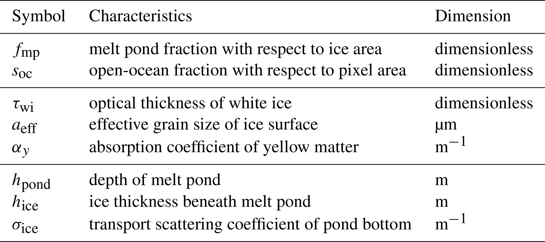
The area fractions soc and fmp are part of the retrieval output. The BRDF of the white ice Rwi is calculated from the inherent optical properties of a stochastic medium using the model of random mixture by Malinka (2014), resulting in three dominant physical parameters: the optical thickness τwi of a surface layer, the mean effective grain size aeff, and the absorption coefficient of yellow matter αy deposited on the ice surface. The optical thickness of the sea ice describes the ability of light to penetrate the ice without being absorbed and is defined by the sea ice texture. The effective grain size is defined as the mean chord length of ice in snow and white ice and is related to the widely used specific surface area (SSA) as
where ρice is the ice density.
To derive the BRDF of melt ponds Rmp, only isotropic reflection from the pond bottom is taken into account, neglecting sideward reflections and deviations from the Lambertian law due to multiple reflections between the pond bottom and surface. Additionally, the meltwater is assumed to be clear, without any contaminants. Although this might not be perfectly true, especially near coastal areas, the effect on the retrieval results in the form of an overestimation of melt pond fraction is estimated to be negligibly small (Malinka et al., 2018). With the mentioned assumptions, three further parameters of importance are determined: the pond depth hpond, the ice thickness underneath the pond hice, and the transport scattering coefficient of that ice σice, defining the spectral albedo of the pond bottom (Malinka et al., 2018).
In combination with the area fractions soc and fmp, these physical parameters dominating the ice and pond surface reflections constitute the state vector
which describes the state of the surface and is optimized in an iterative procedure to find the state that models the measured TOA reflectances the best. In Table 1 an overview of the parameters and their dimensions is given.
3.1 The algorithm structure
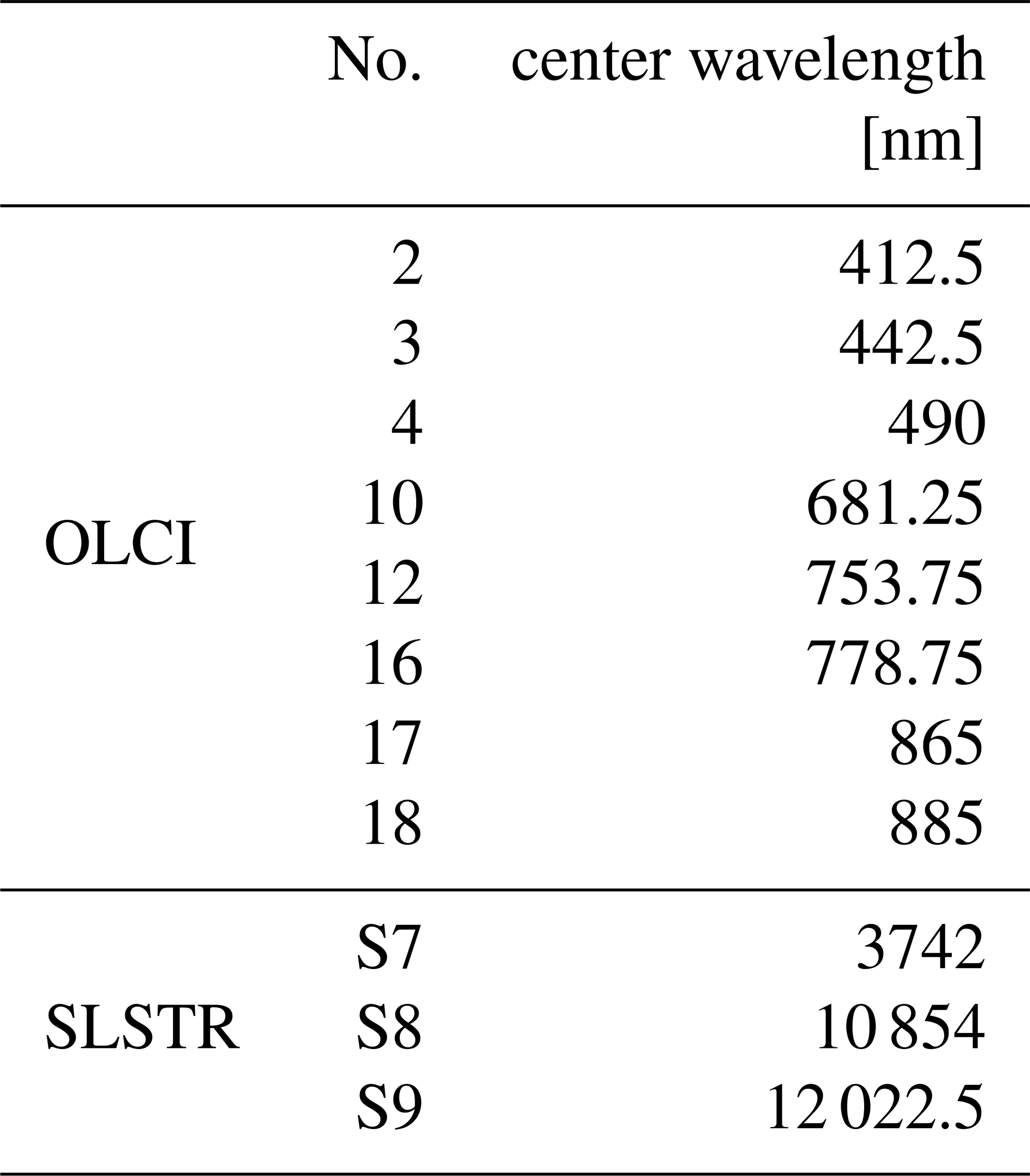
The input data to the algorithm are acquired by the Sentinel-3A and Sentinel-3B satellite instruments OLCI and SLSTR introduced in Sect. 2.1 at a spatial resolution of 1.2 km. From the OLCI the TOA radiances Ri of those channels (Table 2) are used that correspond to the wavelengths of the channels used previously by the MERIS sensor for MPD1 (Istomina et al., 2023). Additionally, the viewing and illumination zenith and azimuth angles are entered into the algorithm. For cloud screening, channels S7, S8, and S9, with the wavelengths given in Table 2, from the SLSTR are used (Istomina et al., 2023).
Table 2OLCI and SLSTR spectral channels used. Channels near 550 nm are excluded in order to avoid the effect of ozone absorption.
As auxiliary input data to set the initial values the allowed range of parameters in X, the OSI SAF drift product and the ERA5 2 m air temperature are used. These data are necessary to calculate the temperature history of every pixel and are inserted into the process block where the initial values and boundaries for the state vector X are set. The details of this procedure are the core of this study and will be discussed in detail in the Sects. 4 and 5. To reduce the input data to pixels where the algorithm is applicable, first a land mask is applied and secondly pixels with cloud contamination are filtered out. To achieve this, cloud screening criteria introduced by Istomina et al. (2010, 2011) and the differential snow index criterion (Zege et al., 2015) are applied. Atmospheric corrections are applied by the use of the radiative transfer code RAY (Tynes et al., 2001) to take into account scattering and absorption by aerosols and gases, as well as molecular scattering; this is explained in detail in Zege et al. (2015). The atmospheric correction block calculates for every pixel the transmission ti and the reflection ri of the atmosphere in the spectral bands i of the wavelengths used. With these, the maximal possible TOA reflectance , in the case of perfect reflection at the surface, is calculated. This value is used in the iterative procedure as a threshold. These values, ti, ri, and , are passed to the iterative procedure in combination with the initialization and the boundaries of the state vector X for all the pixels that are determined to be reasonable pixels for the algorithm. The following description of the iterative procedure is visualized in the flowchart in Fig. 1. It is explained for a single pixel as the processing is independent between pixels.
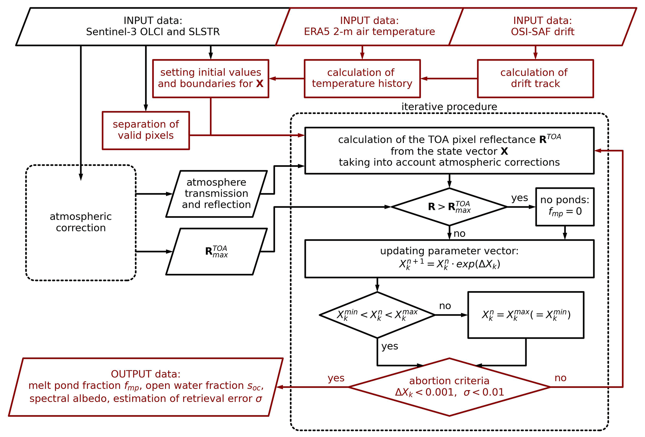
Figure 1Flowchart of the MPD2 algorithm. The atmospheric correction block is left blank in favor of simplicity, and the details can be found in Zege et al. (2015). Red marks parts of the algorithm where major changes have been introduced compared to the MPD1 version. The current iteration step of the optimization process is denoted as n, and k indicates the entries of the state vector X.
-
Starting with the initialized state vector X describing the surface, the TOA reflectances that would be expected are calculated using Eq. (5), the forward model (Malinka, 2014; Malinka et al., 2018) for the BRDF of the white ice and melt ponds, and the transmission and reflectance coefficients of the atmosphere.
-
The measured TOA reflectances in the eight spectral channels i are compared to the reflectance threshold from the atmospheric correction block for the respective channels. If the measured reflectance is higher than this threshold, fmp and soc are zero because melt ponds or open ocean would reduce the measured TOA reflectance. Following, only the parameters describing the white ice reflectance, hpond, hice, and σice, are included in further optimization steps. If the measured reflectance is below the threshold, all parameters of X are included.
-
The state vector is updated according to the differences between the modeled and measured TOA reflectances. This procedure relies on the Newton–Raphson method (Press, 2007). For every component Xk of the state vector and every channel i, the partial derivative of is calculated numerically to compose the matrix M:
With this matrix, the change applied to the components of X is determined from the current iteration step n:
where the vector ΔX is the product of the Moore–Penrose pseudo-inverse (pinv) of matrix M (Press, 2007) and the difference vector between the measured TOA reflectances R and the TOA reflectances calculated in this iteration step Rn:
-
If any updated value of X is beyond the respective boundaries, which were initialized before the iteration process, it is set to the passed boundaries and is no longer included in the remaining optimization process.
-
Steps (1)–(4) are repeated until two abortion criteria are satisfied: the first requirement involves the intended change to the components of X. If the condition
is met for all parameters k, it can be assumed that the algorithm has found a minimum where further iterations would not lead to significant changes in the output. The second condition takes the root mean squared difference σ between the measured and retrieved TOA reflectances into account to ensure that the minimum found can physically describe the surface state.
Finally, the outputs of the retrieval algorithm are the melt pond fraction, open-ocean fraction, and the spectral albedos at wavelengths 400 to 900 nm in 100 nm steps. Additionally, σ, which is an estimator of the retrieval uncertainty for the specific pixel, is provided.
3.2 Algorithm sensitivity to initial values of optimized parameters
The MPD2 algorithm is a complex, multiparameter retrieval. By including open ocean as a third surface type class, the number of free parameters is increased to eight (Table 1). In addition, open ocean is spectrally almost neutral with very little reflectance in the broadband optical and NIR spectrum (Pohl et al., 2020). This can result in a situation in which a mixed pixel consisting of open ocean and bright ice is indistinguishable from a homogeneous pixel of darker ice and makes it virtually impossible to unmix the spectral signals of the surface type components without additional information (Istomina et al., 2023). This additional information could be inserted into the algorithm by finding a suitable initialization and constraint of the state vector X. As the cost function minimized in the retrieval is expected to be multimodal, a suitable initialization of X offers potential to improve the retrieval performance (as the optimization could otherwise run into a false local minimum in the distribution). To investigate the algorithm sensitivity to the initial values of the optimized state vector X, a set of test pixels is selected. For this selection the melt pond fraction product from Sentinel-2, described in Sect. 2.5, is used. After drift correction, the two satellite products overlap and the 10 m resolution Sentinel-2 product (where 120×120 pixel correspond to one of the Sentinel-3 pixels) is used to identify six cases of different dominating surface type classes and their combinations. For each of these six cases, four adjacent pixels of Sentinel-3 (corresponding to an area of 2.4 km × 2.4 km) are chosen, yielding a test bed of 24 intentionally chosen pixels in total. Additionally, six cases of four pixels are chosen randomly. In Fig. 2 the Sentinel-2 reference melt pond fractions are displayed for all 48 test pixels. In the case of the intentionally chosen pixels, the present surface types in these pixels are given, ordered from the highest to lowest fraction. For further discussion, we focus on these manually chosen pixels and average the results for the four pixels representing one case.
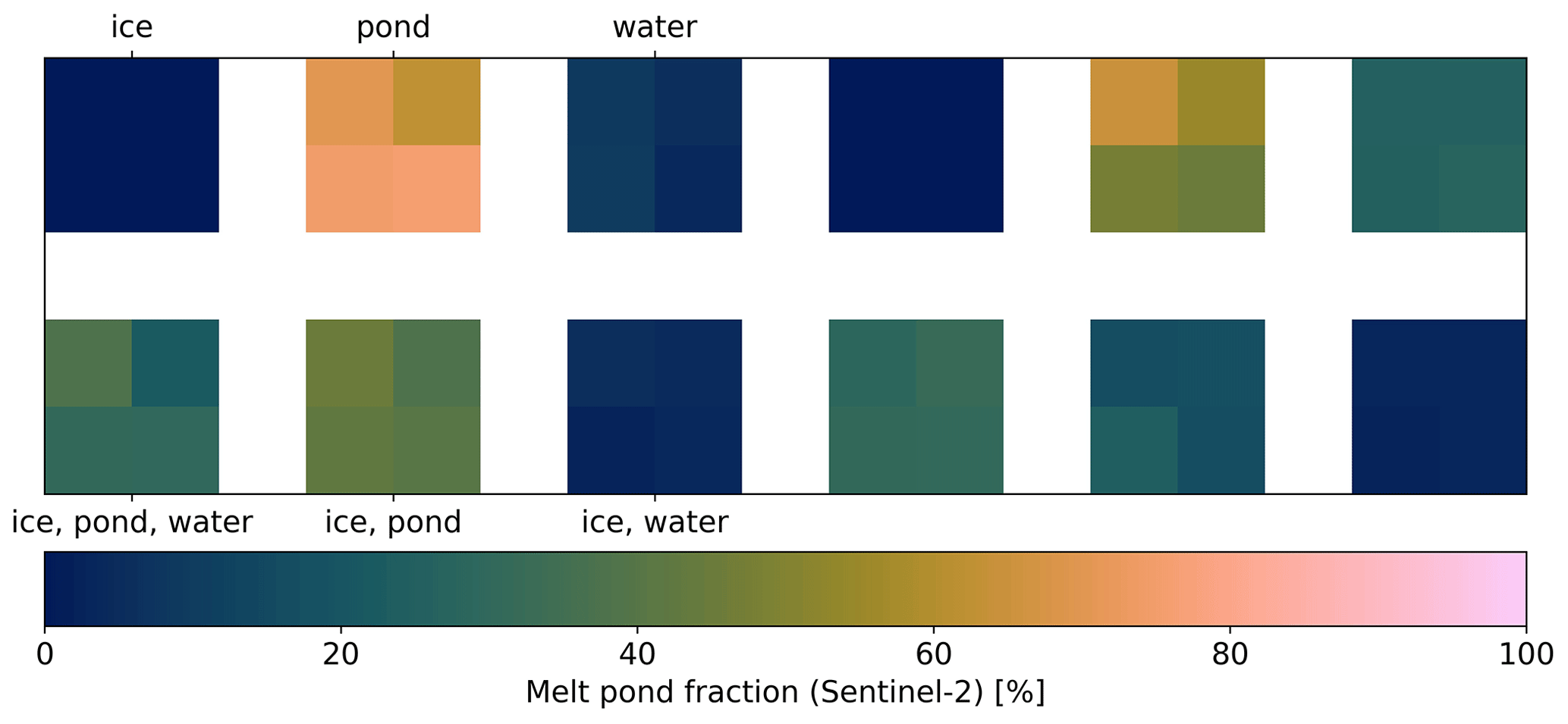
Figure 2Sentinel-2 melt pond fraction reference of the test pixels. Half (right) of the pixels are chosen randomly, and the other half (left) are chosen with the purpose of representing the typical surface types and their combinations as denoted by the labels. In this case, the present surface types in the pixels are listed ordered by their occurrence.
On the Sentinel-3 input data of these test pixels we run a Monte Carlo simulation of the MPD2 algorithm to investigate the retrieval sensitivity to the initial values of the parameters in the state vector X. All parameters Xk are varied simultaneously within according physical ranges. These ranges come from in situ data and can be seen from the limits of the x axes in Fig. 3. This figure shows for each optimized parameter the probability density of retrieving a reasonable result as a function of the initial guess for the different surface type combinations. The definition of a reasonable result is
where mpfMPD2 is the melt pond fraction retrieved with MPD2 and mpfS2 is the reference melt pond fraction of the respective pixel from Sentinel-2. Equation (13) combines the estimation of the absolute and relative error so that for small values of fmp the absolute error needs to be less than 0.1, while for a 100 % melt pond surface the relative error should be below 0.3. Thus, this estimation smoothly transits from the relative difference to the absolute one at small values of fmp.
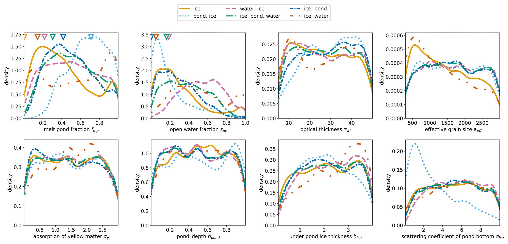
Figure 3Probability densities of initial values yielding a reasonable result for melt pond fraction output. The reasonable output is defined by two criteria: (1) the difference between the melt pond fraction output and the reference value from Sentinel-2 is below 0.1 % or 10 %, and (2) the root mean square deviation (RMSD) of the retrieved reflectances compared to the measured reflectances is below 0.1. The eight panels show the distributions for the different optimized parameters of the state vector X. The differently colored lines represent the average of the four test pixels per dominant surface type (combinations). The triangles in the two upper left panels show the reference values of the melt pond and open-ocean fraction from Sentinel-2.
To analyze Fig. 3 it is important to note that the probability densities are standardized to the number of reasonable results. There are two different ways to look at the graphs.
-
The focus is the difference between the curves representing the surface types. This enables an interpretation of how important it is to choose the initial values for every surface separately.
-
Or the focus is the dependency of a single curve or multiple similar curves on the initial value.
This shows how important the initial values for this case (parameter, surface type) are and can help to choose suitable ones. If there is a strong peak the suitable initialization is important. If the curve is close to a uniform distribution, it is not. For fmp and soc in the two upper left panels of Fig. 3, the differences between the various surface types and combinations are the strongest. The triangles at the top of these two panels give the reference values from the Sentinel-2 product. The comparison of the reference values and the maxima of the probability density curves leads to the conclusion that the retrieval works better when the initial value is already somewhat close to the reality. Interestingly, an initial value of fmp=0 is hardly ever good for the performance of the retrieval. However, it is obvious that the initial value and boundary of fmp and soc should not be fixed but adapted for every pixel to have a higher likelihood of achieving the best result. The effective grain size aeff of sea ice is related to its albedo (Fig. 6) and shows in the upper right panel a strong impact on the retrieval results for the ice and the ice–water surfaces, the latter of which is also strongly dominated by ice. For the other surface types aeff seems to have little impact on the retrieval performance. Another noticeable feature is the strong peak at small scattering coefficients σice for ponded pixels in the lower right panel, while all other surface types show almost a uniform distribution. This is neglected because we expect the influence of the initial value for σice to decrease with other parameters being constrained. For the other optimized parameters, τwi, αy, hpond, and hice, the dependency of the probability of a reasonable result on the initial values is not as strong. Based on this analysis, we conclude that an approach is needed to initialize and constrain fmp and soc as well as aeff. In the following two sections constraints for (1) aeff and τwi, which are correlated, as well as (2) fmp and soc are developed.
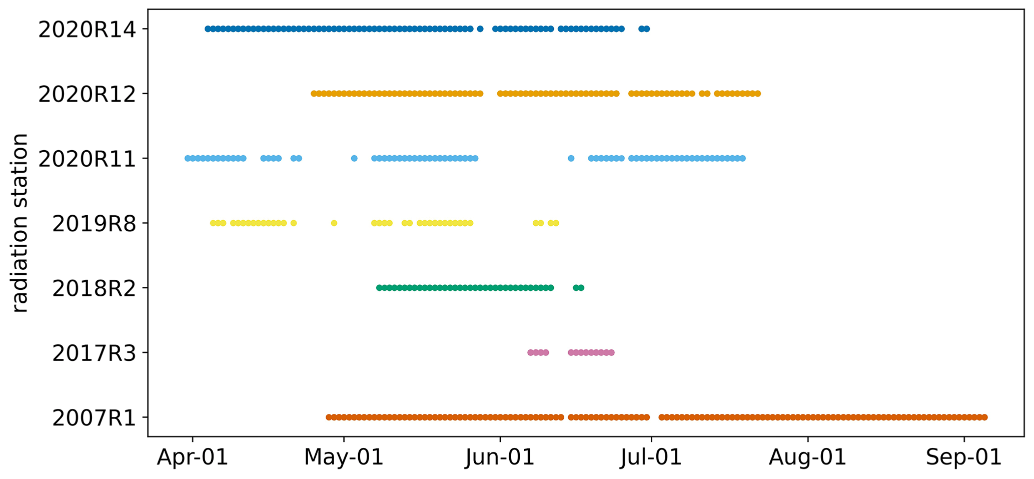
Figure 4Overview of the available radiation station data throughout the summer period after data filtering. The first four digits of the station names indicate the year of observation.
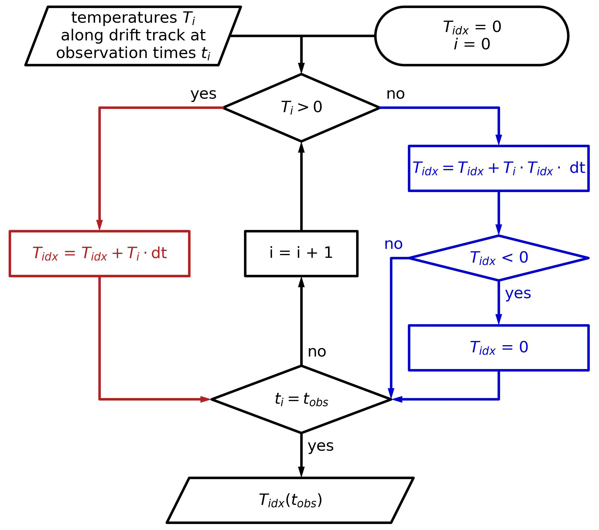
Figure 5Flowchart of the calculation of the temperature index Tidx at any time of observation tobs. i iterates through the times steps of size dt. As Tidx is initialized at 0, it is important that the beginning of this iteration (observation) period lies before the start of any melting.
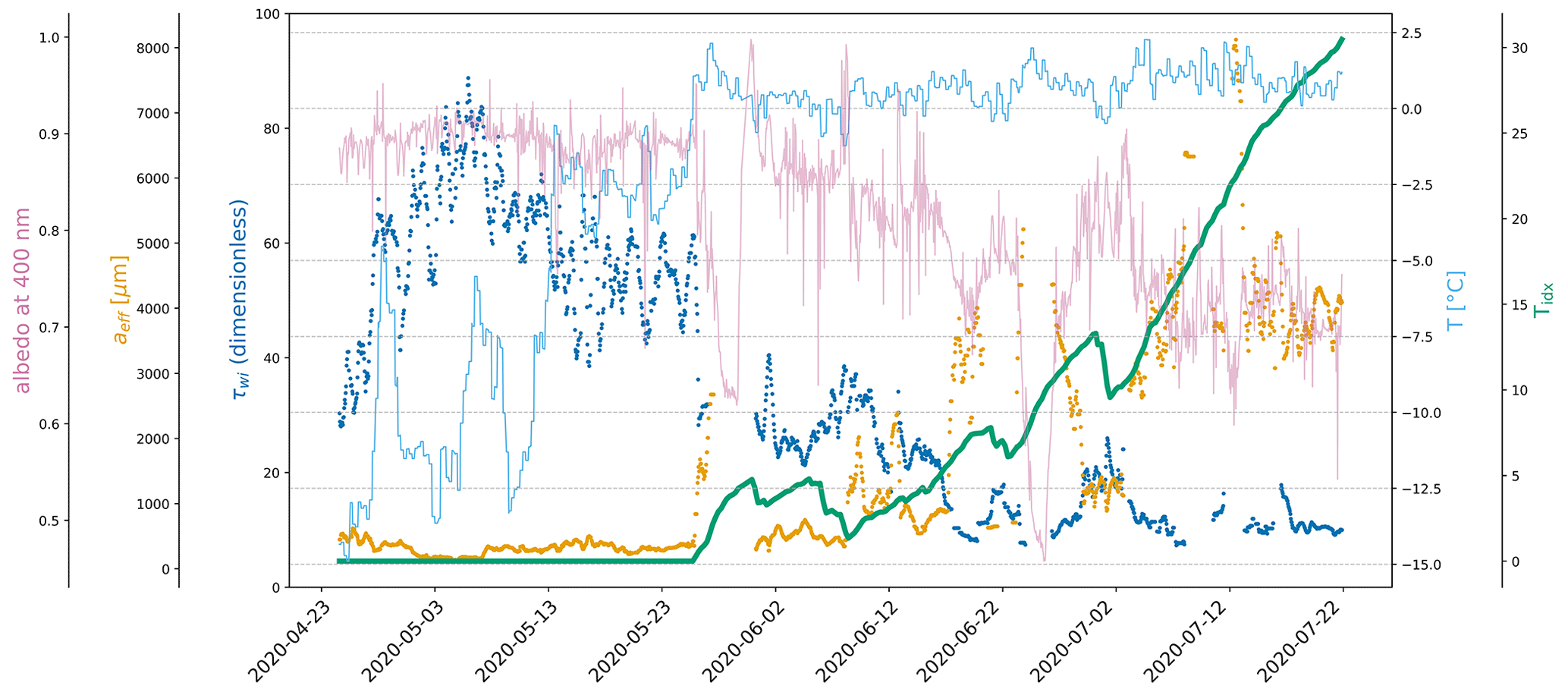
Figure 6Albedo at 400 nm (pink, thin solid line) measured by the radiation station 2020R12, effective grain size aeff (orange, dots) and optical thickness τwi (dark blue, dots) retrieved from the spectral albedo measurements of the radiation station, 2 m air temperature (light blue, thin solid line) from ERA5, and the temperature index Tidx (green, thick solid line) derived from the air temperature.
The reflective properties of sea ice are highly variable. In April and May, most of it is covered by snow featuring a very high albedo. This is because dry snow consists of small grains, typically around 100–300 µm (Jäkel et al., 2021), leading to high (almost infinite) optical thickness and strong scattering (Perovich, 1979). When the air temperature approaches the melting point, the surface becomes wetter and snow grains start to bond (Marsh, 1987) in a process called sintering (Blackford, 2007). Thereby the snow grain size increases and the optical thickness of the surface layer becomes finite. Once the snow is melted and drained into surface depressions to form melt ponds, white ice is left. The reflection of this ice is defined by a surface scattering layer (Grenfell and Maykut, 1977) and can be described by the same metrics as snow (Zege et al., 2015; Malinka et al., 2016). However, the grain sizes are much larger and the optical thickness is reduced. It is eminent that the effective grain size aeff and optical thickness τwi of a sea ice surface layer (consisting of white ice or snow) are correlated and define the albedo. Moreover, they depend on the wetness of the surface and thus on the air temperature. The goal of this section is to find a simple relation between the temperature history that the sea ice experienced and the physical properties aeff and τwi. For that purpose, the satellite spectral measurements of the surface reflectance are no longer considered a snapshot in time but the result of the previous history of that surface. That means the drift trajectory of every single satellite pixel is calculated from the time of measurement back to the beginning of the melt season using the OSI SAF drift product described in Sect. 2.2. Along this drift track the 2 m air temperatures are collected from the ERA5 product described in Sect. 2.3. The empirical relation found between the temperature history along the drift track and the optical properties is based on in situ spectral albedo measurements introduced in Sect. 2.4. The development and filtering of these data are described in Sect. 4.1. Afterwards, in Sect. 4.2, the correlation between temperature history and optical surface properties is explored and discussed.
4.1 In situ data preparation
We use spectral albedo measurements from in situ radiation station data introduced in Sect. 2.4 to develop the relationship between temperature history and surface optical properties. It is necessary to make sure that only albedo measurements of sea ice and not of melt ponds are used for this analysis because aeff and τwi are not appropriate properties to describe melt pond reflection. For this purpose, we use a conservative threshold applied to the ratio of the albedo at 500 and 900 nm, which is sensitive to the water content of the surface (Nicolaus et al., 2010; Tao et al., 2023). If the ratio is >1.5, the data are removed from the evaluation because there is most likely a melt pond in the observation area. Then the forward model used in the MPD2 algorithm itself and described in Malinka et al. (2016) is used to derive aeff and τwi from the in situ spectral albedo measurements. The model output comes along with an uncertainty estimate which is used to filter out measurements where the model was not able to reproduce the observed spectra sufficiently and thus the derived values of aeff and τwi are not reliable. Additionally, we use an averaged slope of the albedo curve in combination with the albedo at 400 nm to eliminate observations where aeff is inexplicable high, probably because of irregular sky conditions of an undetected melt pond for which the model is not valid. Subsequently, events of fresh snowfall after the melting had already started are removed from the in situ dataset as these are not covered by the forward model. This is done by the application of a lower threshold of 300 µm <aeff to the effective grain size according to Jäkel et al. (2021). Figure 4 shows the time periods during which observations are available after these steps of filtering.
4.2 Relation between the physical properties and the temperature history
To relate the modeled aeff and τwi to the temperature history dictating the current state of the sea ice surface we decided to use the approach of the cumulative melting degree day (CMDD) index, which is defined as the integrated temperature above 0 °C over time. To be able to take into account short freezing periods in between the melting periods, we adapted the conventional CMDD index, resulting in an index we call Tidx. Starting at the beginning of observations, or at the date where the backtracking of a pixel ends, the temperature is evaluated at every time step ti to add to or subtract from the current value of the temperature index Tidx. It is important that this starting date of calculations lies before the melt onset. Figure 5 shows the iterative procedure that is used to gain the temperature index Tidx at any time of observation tobs. This procedure takes a list of temperatures along the back-projected drift trajectory of a pixel (observation) and comprises two blocks, one handling the melting temperature (left, red part) and the other handling the freezing periods (right, blue part). If the temperature is above 0 °C the common definition of cumulative melting degree days (CMDD) is used:
When the temperature drops below 0 °C, Tidx is reduced in proportion to the time period, magnitude of negative temperature, and current value of Tidx. This approach is based on the assumption of the surface getting drier when it is freezing again, stopping the sintering and leading to a slight refinement of the grains. As soon as the temperature rises again above 0 °C, we switch back to the increase in Tidx following the CMDD definition in Eq. (14).
As an example, Fig. 6 shows the modeled physical quantities aeff and τwi together with the 2 m air temperature T and the derived temperature index Tidx for the radiation station 2020R12. With an overall increasing Tidx, the optical thickness of the surface layer decreases while the effective grain size increases. Strong fluctuations are especially visible for the modeled grain size corresponding to different thickness of the scattering layer. There are two distinct data gaps in the modeled data at the end of May and around 25 June. This is where the data have been filtered out because of the likely presence of melt ponds (Nicolaus et al., 2010). Around these two gaps, the scatter is especially high, showing the strong surface variability close to melting and freezing conditions.
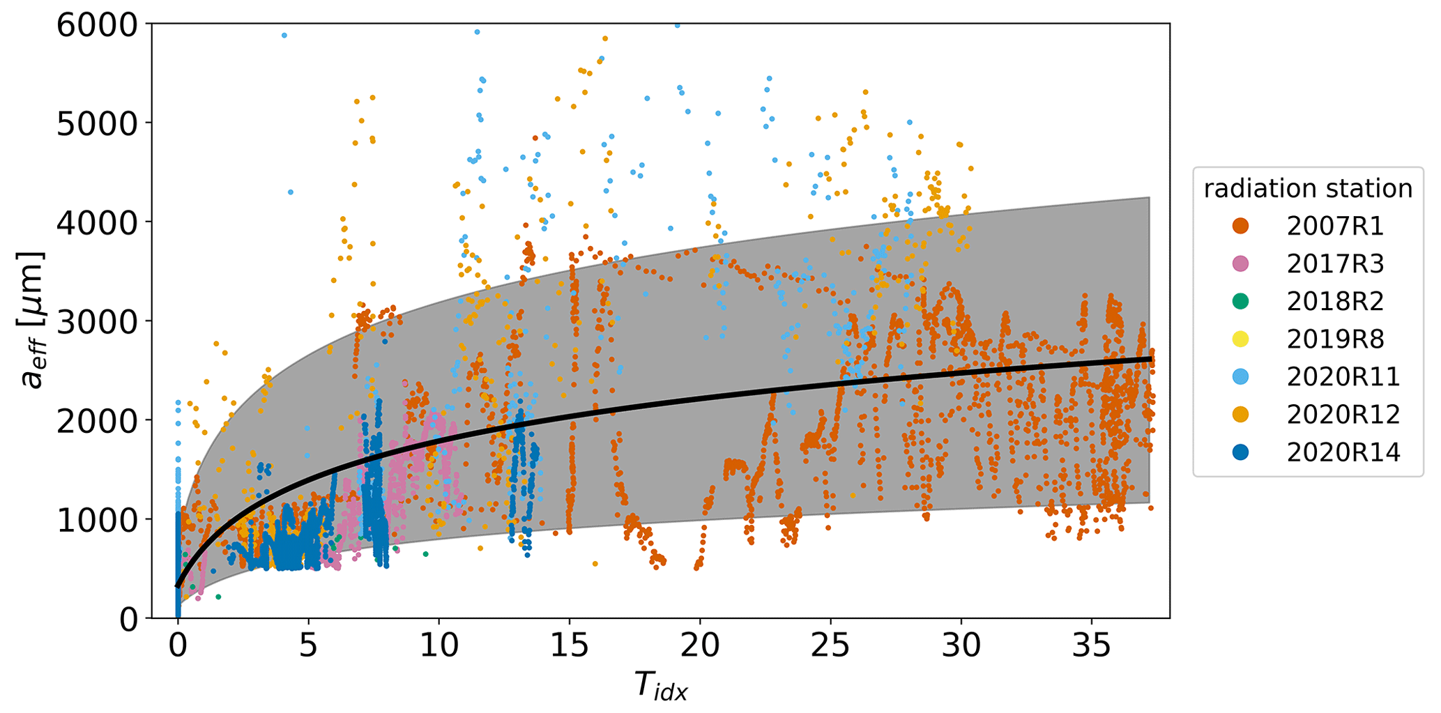
Figure 7Scatter plot of modeled optical thickness aeff depending on the temperature index Tidx. The different colors indicate measurements of different radiation stations. The thick black line is the fit to all data, which we later use to determine the initial value of aeff depending on Tidx. The gray area marks the allowed values limited by the upper and lower boundaries derived from the 95th and 5th percentiles.
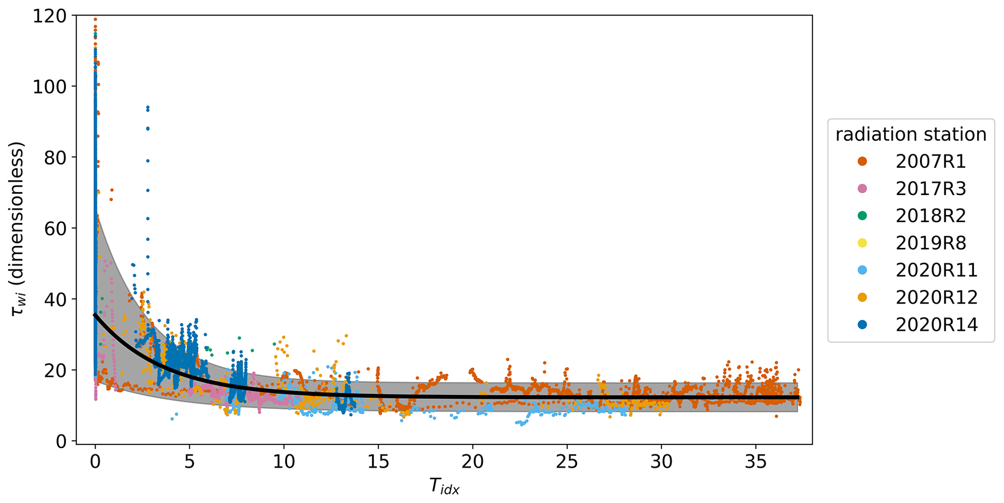
Figure 8Scatter plot of modeled optical thickness τwi depending on the temperature index Tidx. The different colors indicate measurements of different radiation stations. The thick black line is the fit to all data, which we later use to determine the initial value of τwi depending on Tidx. The gray area marks the allowed values limited by the upper and lower boundaries derived from the 95th and 5th percentiles.
The physical properties aeff and τwi as a function of the temperature history are shown in Figs. 7 and 8. Here, the observations of all measurement stations are combined, with the color indicating the radiation station according to the color code in Fig. 4. We use the following fit functions to describe their relations.
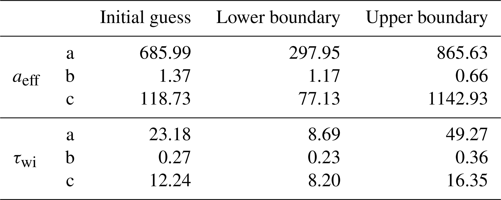
These fits are applied to the full dataset to determine the initial value of the respective parameter as a function of the temperature index. This initial value function we will later use in the MPD2 retrieval. To get upper and lower boundaries also as a function of Tidx, we use the 95th and 5th percentiles of the data. The resulting fit parameters a, b, and c for both properties are given in Table 3. In Fig. 7, aeff features low values at Tidx=0. With increasing Tidx, aeff also increases as does the scatter, which is covered by the increasingly wider range of allowed values marked by the light gray area. For τwi there is a lot of scatter visible at Tidx=0 in Fig. 8. This is covered by the wider range of allowed values marked by the light gray area. With increasing Tidx, there is less variability and the optical thickness converges at a lower value. Overall the dependence is not as strong as for aeff, which is expected from the sensitivity analysis in Sect. 3.2.
Table 3Fit parameters to describe initial values and lower and upper boundaries for the optical thickness τwi and the effective grain size aeff.
The spectral albedo of sea ice, melt ponds, and open ocean features large variability. Even though the transition of the spectra going from wet ice surfaces to light and shallow melt ponds is relatively fluent, there is great potential in the spectral measurements to differentiate between the difference surface types given they are observed separately. Whereas melt ponds have a much lower albedo in the NIR (0.1–0.2) than in visible wavelengths (0.4–0.7), unponded, dry ice shows few changes in albedo in the visible blue range (0.7–1.0) and only a slight decrease towards the NIR (0.6–0.9) (Istomina et al., 2015a; Malinka et al., 2018; Light et al., 2022). As this spectral behavior is dictated by the amount of liquid water in the surface layer, the spectrum of sea ice gets closer to the spectrum of a light melt pond, the wetter it is. A similar situation applies to wet snow which has a lower albedo in NIR and complicates distinguishing the surface types even more. Open ocean has a constant low albedo below 0.1 (Pohl et al., 2020) in the visible and NIR range. However, at the 1.2 km spatial resolution of the Sentinel-3 sensors, as the situation becomes sub-pixel, it is complicated to disentangle the spectral signals of the mixed surface types (Istomina et al., 2023), which themselves already feature large variability. In particular, different compositions of surface fractions of ice, melt ponds, and open ocean can result in the same mixed spectral signal at 1.2 km resolution if boundary conditions for, e.g., the snow grain size (larger grains reduce the albedo of the ice surface type), are not taken into account. Yet, there is the potential to get a good first guess of the composition of the surface types, which will be sufficient as an initialization of the physical MPD2 algorithm. In this section, we develop a first-order empirical retrieval of melt pond and open-ocean fractions to use as initial values for the MPD2 algorithm. This empirical retrieval is based on the same TOA reflectances also fed into the physical MPD2 retrieval algorithm. The empirical retrieval is developed on the 48 test pixels described in Sect. 3.2 and comprises two steps. First, we define the brightness h of a pixel as the average TOA reflectance in the spectral bands shown in Fig. 9. This value is used to estimate the total water fraction in the pixel without distinguishing between melt ponds and open ocean. This will be discussed in Sect. 5.1. Second, we define the slope of the spectrum from the reflectance difference between 490 and 754 nm. From this value the proportion of melt ponds and open ocean relative to the total water fraction is estimated, as presented in Sect. 5.2.
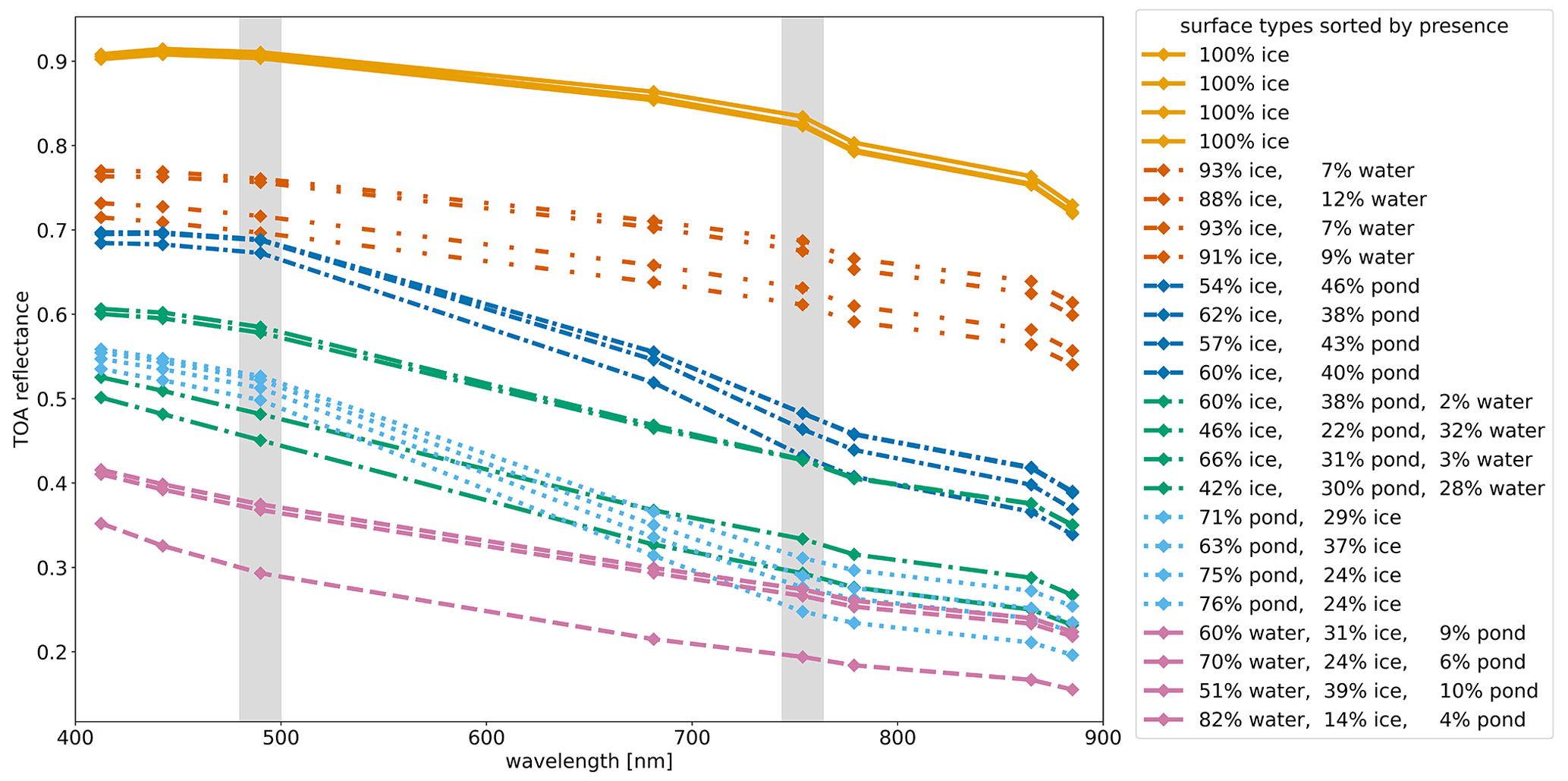
Figure 9TOA reflectance spectra measured by the OLCI on the Sentinel-3 satellite for the 24 test pixels with known dominant surface types (Fig. 2, left part). These are indicated by the color and style of the lines connecting the measurements at eight different wavelengths. Additionally, the percentage of the surface types, known from the Sentinel-2 reference product, is given. The vertical gray areas mark the spectral bands used for the definition of the slope of the spectra in the empirical pre-retrieval.
Note that in spite of the difference between albedo and reflectance, as well as between in situ and TOA measurements, we neglect both differences in this section because we only estimate the initial values and constraints empirically and more accurate values will be achieved in the retrieval iteration cycle.
5.1 Brightness criterion: estimation of total water fraction
The brightness h of a pixel is defined as the TOA average reflectance in the eight spectral bands shown in Fig. 9, which includes atmospheric influence and serves as a rough empirical estimate: as sea ice is a much better reflecting surface than melt ponds or water, this quantity can be used to separate water and ice surfaces and thereby estimate the total water fraction twf. This is the area fraction of a pixel that is covered either by melt ponds or by the open ocean. We set a fixed threshold hmin on the brightness below which we assume the pixel to contain only water and no sea ice that is not covered by ponds. The upper threshold hmax above which the pixel contains sea ice only is expected to depend on the time of the year and region of observation. This is because of the evolution of sea ice reflective properties with time and temperature (Marsh, 1987). Thus, we again use the temperature index Tidx defined in Sect. 4.2, as the temperature describes the seasonal cycle and regional differences while observing exceptional weather situations. With increasing Tidx, the sea ice surface comprises larger grain sizes, i.e., becoming wetter and thus less reflective but still considered to be pure ice surface.
The dependency in Eq. (18) is determined from the in situ spectral albedo measurements described in Sects. 2.4 and 4.1. The brightness h of the measurements is calculated from the wavelengths matching the spectral channels of the OLCI used in the MPD2 algorithm. Then a linear fit is applied to extract a simple dependency and define a limit above which it can be assumed that there is only sea ice observed. The inlay in Fig. 10 shows a density plot of the brightness h as a function of Tidx and the linear fit.
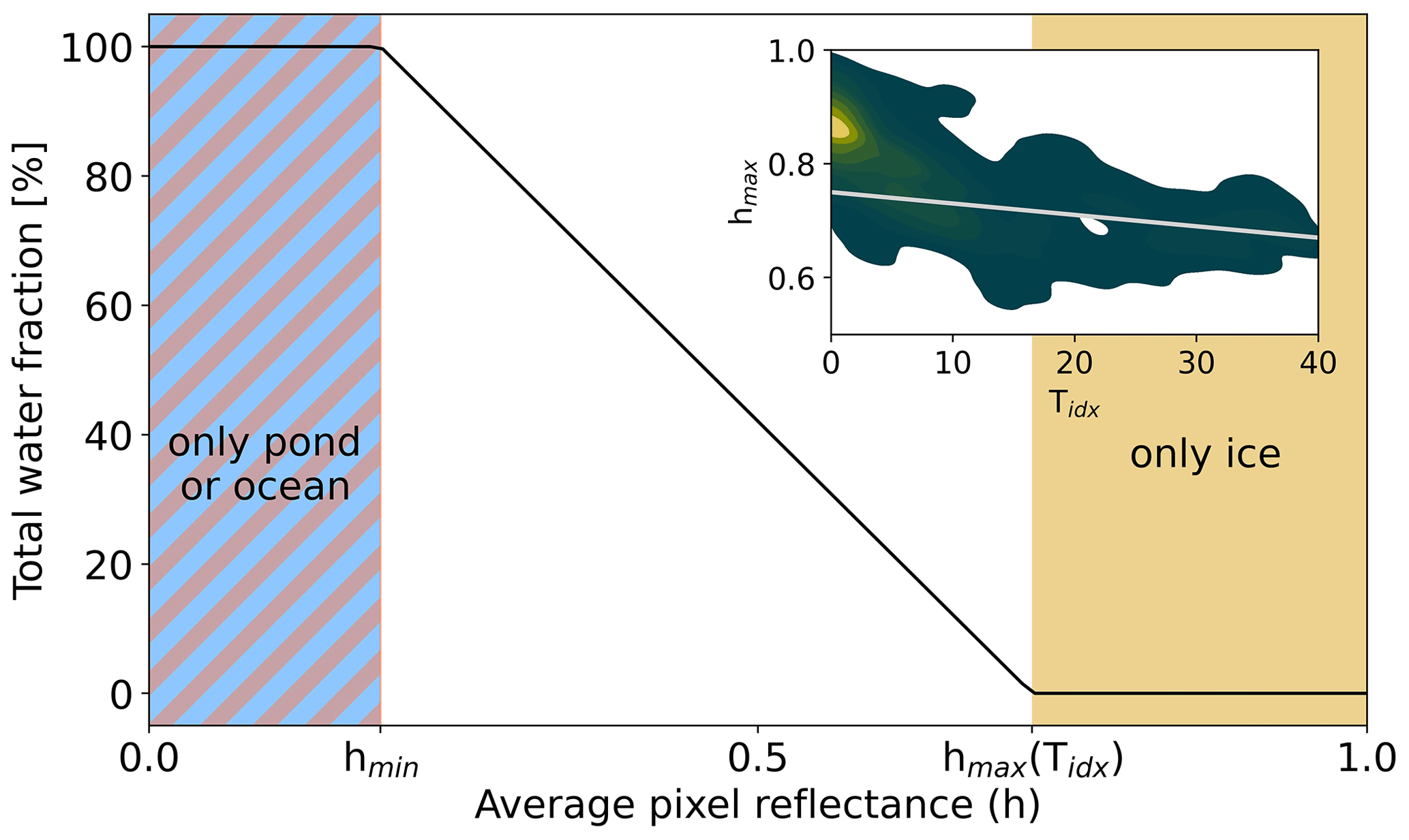
Figure 10Main figure: total water fraction twf as a linear function of the pixel brightness h (average of TOA reflectances used) between the lower threshold hmin below which the pixel is fully covered by water surfaces and the upper threshold hmax above which the pixel comprises only unponded sea ice surface. This threshold is a function of the temperature index Tidx. Inlay: the dependency of hmax on the Tidx derived from in situ spectral albedo measurements. Displayed is a density plot of the in situ data and a linear fit (gray line) describing the threshold above which the surface is so bright that it is expected to be sea ice only, changing with Tidx.
Between the lower hmin and the upper threshold hmax, corresponding to a pure water and pure sea ice pixel, respectively, a linear transition is assumed:
This yields the total water fraction twf as a function of the pixel brightness h as shown in Fig. 10.
5.2 Slope criterion: separation of melt ponds and open ocean
The slope s for a satellite pixel is defined as the absolute ratio between the spectral reflectances at 490 and 754 nm. These two channels are marked by the vertical gray areas in Fig. 9. The choice of these channels is based on the well-investigated reflectance difference of sea ice and melt pond between the blue and red–NIR range (Rösel et al., 2012; Wang et al., 2020). We decided to use the channel at 753.75 nm instead of any other channel because for longer wavelengths the ice reflectance shows a stronger decrease, which would reduce the difference to the melt pond class (Fig. 9). Based on s we now derive the pond fraction pf and the ocean fraction of. These quantities are defined relative to the total water fraction twf and not to the pixel. Thus, the following explanation can be cut to the derivation of pf only because it is then defined by
As shown in Fig. 11, we assume a linear transition based on s between the case of a 100 % ocean-covered pixel (below smin) and a 100 % melt-pond-covered pixel (above smax).
Again, we make use of Tidx to take care of the seasonal and regional differences, mainly driven by the air temperature history. In this case, both thresholds depend on Tidx and additionally on the twf. This is because the twf determines the fraction of the spectrum that is defined by the melt pond and open-ocean mixture: if twf is very small, the pixel spectrum will be dominated by the sea ice surface and have a small s, even though the small amount of water might be melt ponds with large s. Figure 12 displays the linear dependency of the upper and lower threshold smin and smax on twf. If there is almost no water in the pixel, the spectrum is fully dominated by the sea ice and it is impossible for the small amount of water to distinguish between open ocean and melt ponds. This is one of the major issues of this empirical approach. However, it is a common problem to separate melt ponds and open ocean from moderate-resolution spectroradiometers, like on Sentinel-3 or MODIS, in the presence of sea ice because of the spectral neutrality of open ocean (Rösel and Kaleschke, 2011; Istomina et al., 2015a, 2023). The value of s in the case of a pure sea ice surface is derived as a function of Tidx from the in situ spectral albedo measurements. This dataset provides spectra of sea ice surfaces only related to Tidx, from which the slope s can be calculated. The inlay in Fig. 12 shows a density plot of these data with a linear fit of the average observed slope sice(Tidx). The other extreme case is the complete absence of sea ice surface in a pixel. This further separates into two possible extreme cases.
-
The sea ice is fully pond-covered. For this case we found a threshold of spond=0.605 to be suitable.
-
The pixel contains only open ocean. For this, a value of socean=0.264 proved to be suitable.
These values are derived by testing combinations of these values in a reasonable range on the test pixels and then evaluating the results in comparison with the Sentinel-2 reference scenes. Note that these values relate to TOA reflectance observations, where the atmospheric effect might lead to deviations from in situ literature observations. Between the three tie points of extreme (pure surface type) cases, linear functions are used to describe the thresholds.
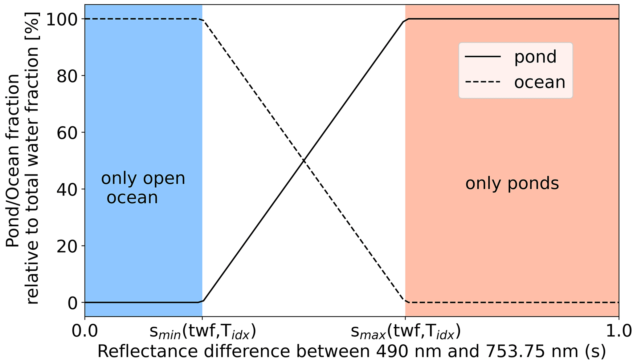
Figure 11Pond fraction (solid line) and ocean fraction (dashed line) as a function of the spectrum slope s and given relative to the total water fraction twf. Below the threshold smin, all water in the pixel is open ocean. Above the threshold smax, all water in the pixel is in melt ponds. Both thresholds depend on Tidx and twf.
5.3 Results of the empirical retrieval
Putting together the estimation of the total water fraction and the separation of melt ponds and open ocean, we derive the desired quantities.
With this, the estimate of fmp and soc is improved from using constant values (Fig. 13, upper row) to pixel-wise adjusted values (Fig. 13, middle row). Compared to the reference values from Sentinel-2 (Fig. 13 bottom row), the uncertainty is reduced from above 20 % to approximately 10 % within the test pixels. This is expected to be sufficient to function as an initialization for fmp and soc for the MPD2 physical retrieval. Despite the lower uncertainty of the initialization values, the boundaries are set looser to ±25 % of the initial values.
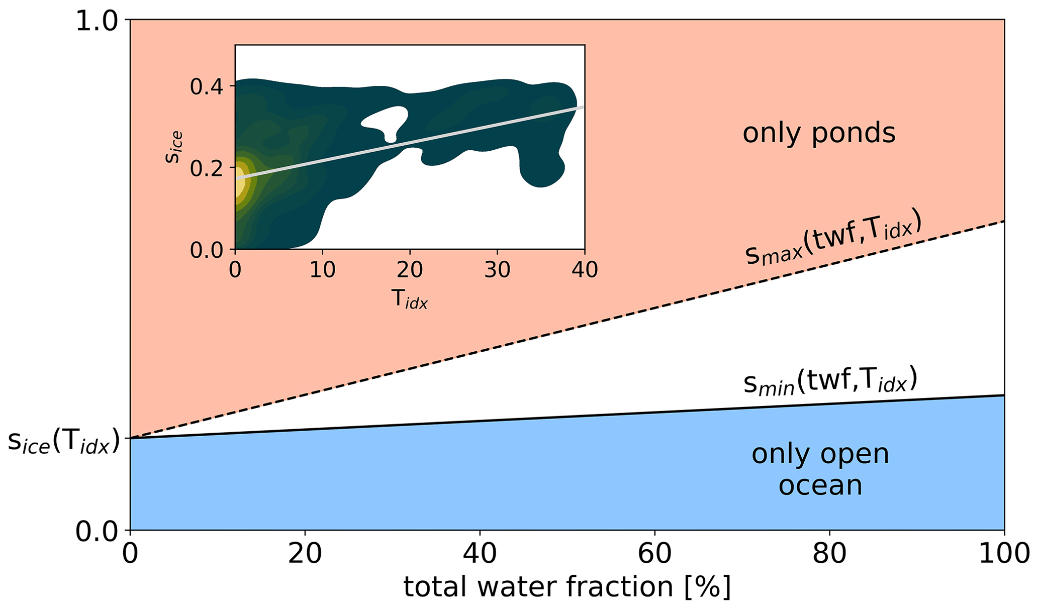
Figure 12Main figure: lower threshold of the spectrum slope smin (solid line) below which all water is assumed to be open ocean and the upper threshold smax (dashed line) above which all water is in melt ponds as a function of twf. Inlay: the dependency of sice on the Tidx derived from in situ spectral albedo measurements. Displayed is a density plot of s derived from in situ data and a linear fit (gray line) of the average slope of the ice surfaces sice as a function of Tidx.
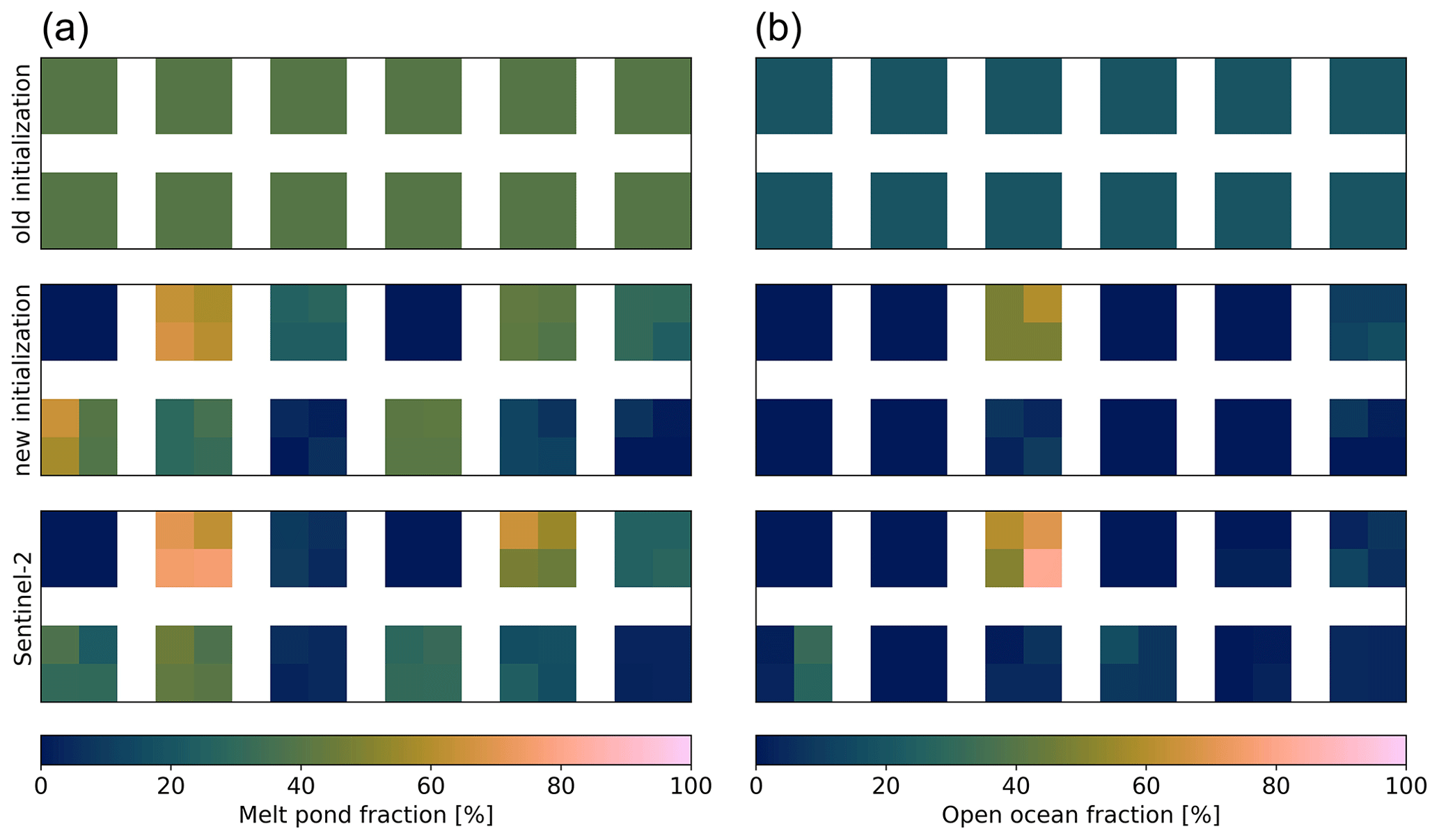
Figure 13Melt pond fraction (a) and open-ocean fraction (b) of the test pixels (see Fig. 2). The upper row displays the previously used constant initialization of 40 % and 20 % for fmp and soc, respectively. The middle row displays the new pixel-specific initialization. The lower row shows the reference from the Sentinel-2 data product.
6.1 Evaluation on test pixels
The new initialization of the four parameters aeff, τwi, fmp, and soc (Sects. 4 and 5) is applied in another Monte Carlo simulation on the 48 test pixels introduced in Sect. 3.2. For the remaining parameters the same random seed is used as before, and also the number of runs is the same. Based on these simulations, the optimal initial values and constraints for the remaining parameters can be established. These values are not adapted pixel-wise but fixed as constants (Table 4) and are used for the entire Arctic and season. All parameters with their initial values and boundaries are given in Table 4. To evaluate the improvement achieved by the newly developed pixel-dependent initializations, we again use the definition of reasonable results with the thresholds as defined in Sect. 3.2. Figure 14 shows the percentage of the results that are reasonable with and without the new initializations. Additionally, the average deviation of fmp compared to the Sentinel-2 reference is shown.
Table 4Overview of the initial values, boundaries, and increments of optimized parameters.
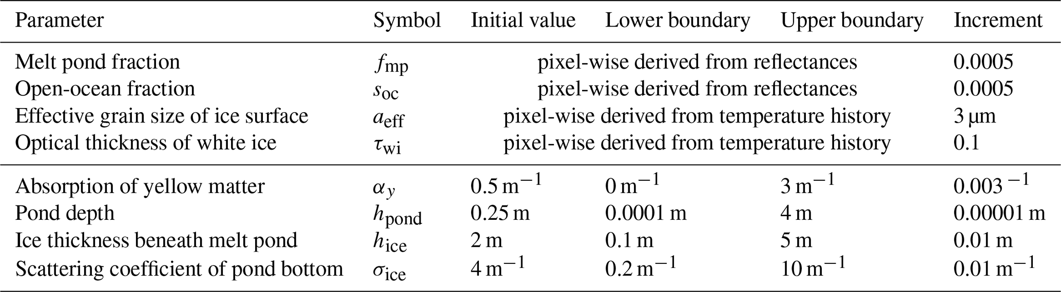
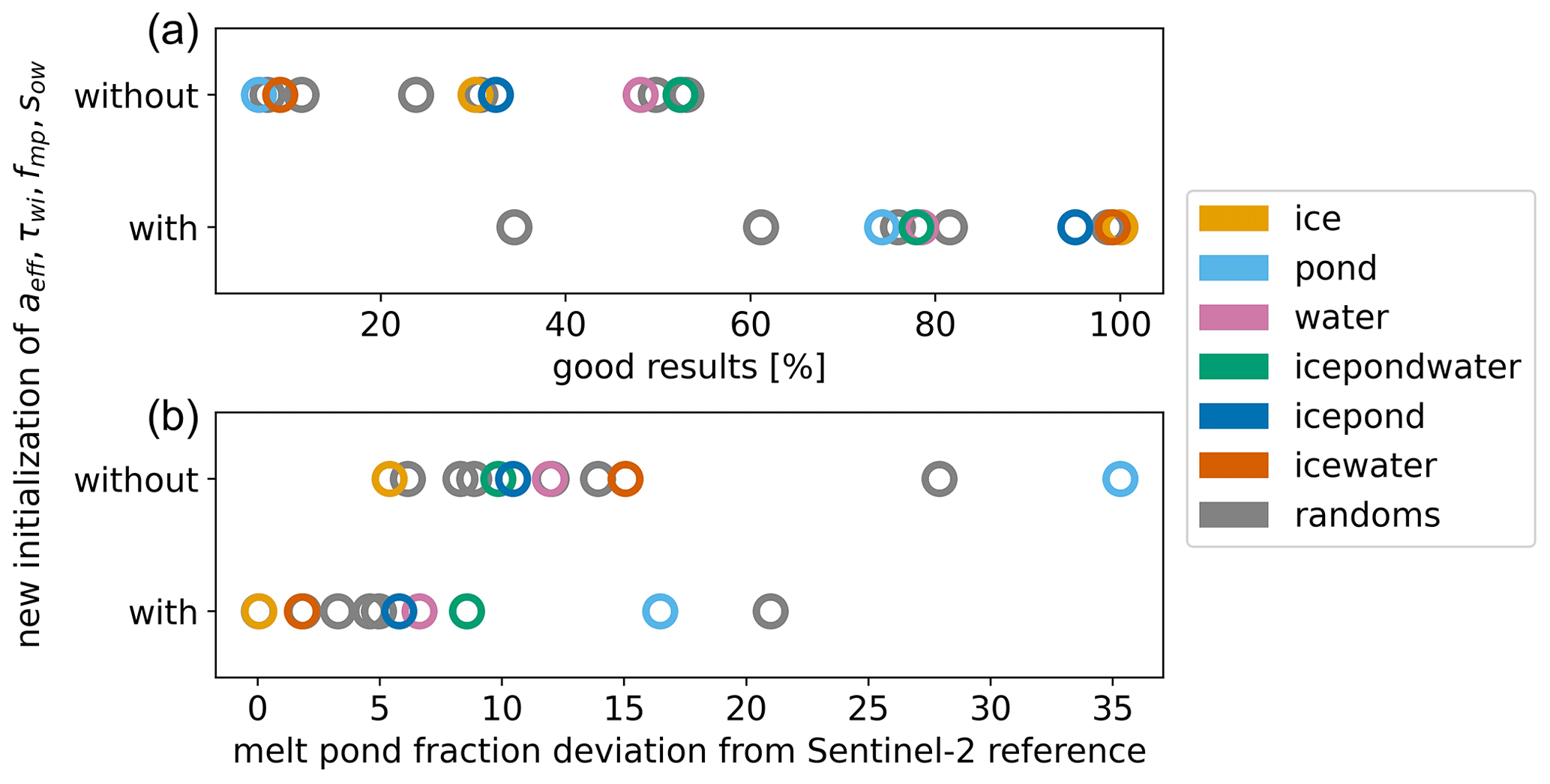
Figure 14Comparison of the Monte Carlo simulation results with and without the new initialization of aeff, τwi, fmp, and soc. The upper panel shows the percentage of the runs that gave a reasonable result. The lower panel shows the average deviation of the retrieved fmp compared to the Sentinel-2 reference. The colors indicate the assigned and the random surface type pixels that were used in the simulations.
By using the new initialization for the four parameters, the number of reasonable results has increased from an average of 30 % of the 30 000 runs to an average of 81 %. The improvement is visible for all assigned surface type combinations as well as for the randomly chosen test pixels. Also, the deviation of fmp compared to the Sentinel-2 reference dataset is reduced in all cases. Especially for strongly ponded pixels the improvement is pronounced, while still featuring the largest deviations. On average, the deviation within these test pixels was reduced from 14 % to 6 %. However, an improvement can be expected when looking only at the test pixels that were used to develop the new initializations and constraints. Therefore we will look at the independent Sentinel-2 reference dataset next.
6.2 Comparison to Sentinel-2 reference
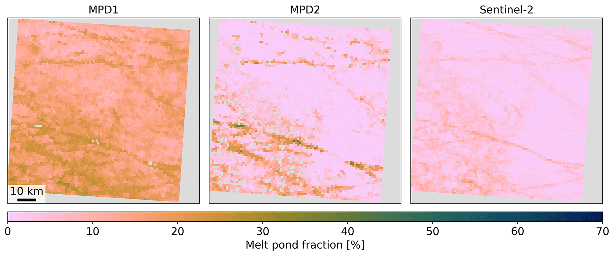
The new initialization is used for processing the Sentinel-3 data of all the occasions, where the Sentinel-2 reference dataset provides data. The possible time difference between the satellite overflights is regarded by the drift correction. Because of the time difference and varying cloud coverage some observations are discarded if there are no overlapping data left. The same data are processed with the former version of the retrieval, i.e., MPD1. Figure 15 shows an example map of fmp derived with MPD1 and MPD2 compared with the Sentinel-2 reference product. Figure 16 shows soc derived from MPD2 compared with the Sentinel-2 product for the same example case.
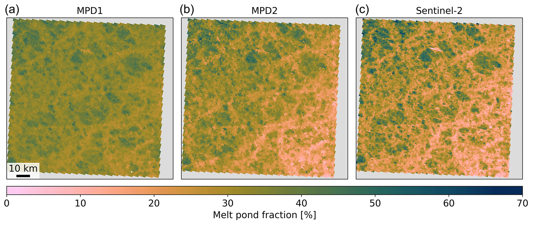
Figure 15Regional maps of melt pond fraction fmp derived with the former algorithm MPD1 (a), the new retrieval version MPD2 (b), and the Sentinel-2 reference product (c). Shown is an example from 3 July 2017 close to Queen Elizabeth Islands at approximately 79° N and 120° W. All maps share the same scale and color map.
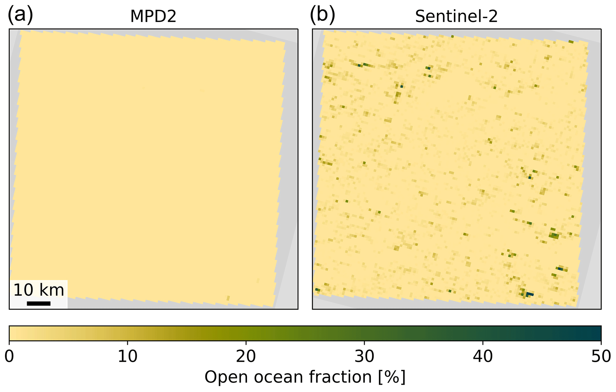
Figure 16Regional maps of open-ocean fraction soc derived with the new algorithm version MPD2 (a) and from the Sentinel-2 reference product (c). Shown is an example from 3 July 2017 close to the Queen Elizabeth Islands, at approximately 79° N and 120° W. Both maps share the same scale and color map.
The right panel of Fig. 15 shows the reference fmp from Sentinel-2 scaled down to the 1.2 km resolution of the MPD products. Despite the downscaling, it contains higher-resolution information, leading to greater detail. The left panel shows the result from the MPD1 version. It covers a much smaller range of fmp, smoothing the details and missing the overall tendency of higher fmp in the upper left trending towards lower values in the lower right. This trend is much better resolved by the MPD2 version, which is displayed in the middle panel of Fig. 15.
soc is only retrieved with the MPD2 algorithm and is not available for MPD1; thus, only the MPD2 soc can be compared to Sentinel-2 in Fig. 16. The results for this case consistently show very low open-ocean fractions. However, in the Sentinel-2 product few very small open-ocean spots are detected which could not be resolved at the low resolution of the Sentinel-3 data used in by the MPD2 algorithm.
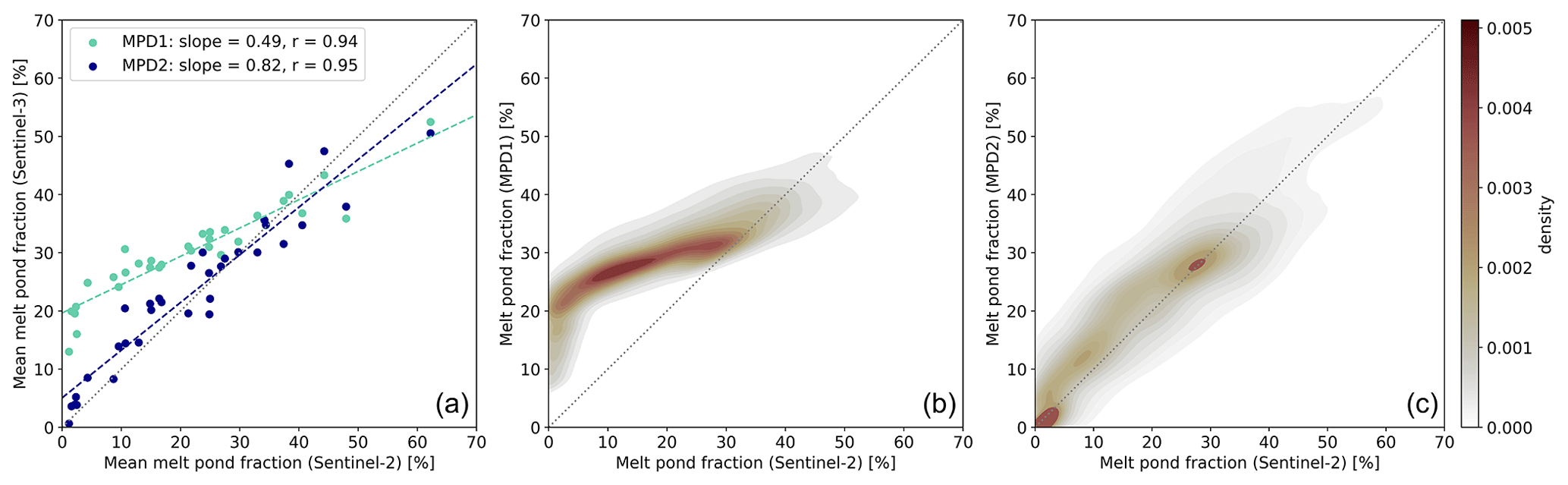
Figure 17(a) Scatter plot of melt pond fraction fmp derived with MPD1 (cyan) and MPD2 (blue) against the Sentinel-2 reference product, averaged per Sentinel-2 scene. The dashed lines show a linear fit to the data points, and the dotted line indicates the identity line. As a measure of quality, the slope and the correlation coefficient r are specified. (b, c) Density plots of fmp derived with MPD1 (b) and MPD2 (c) against the Sentinel-2 reference product, compared pixel-wise after drift correction. The color scale is normalized such that the area sums up to 1 and is valid for both densities.
Figure 17 shows the comparison of the retrieved MPD1 and MPD2 fmp with all Sentinel-2 reference scenes. The scatter plot (left) shows the average values of the 33 scenes. While the MPD1 algorithm (cyan) struggles with low melt pond fractions, MPD2 (dark blue) shows improved results with consistently low retrieved pond fractions. In general the results with MPD1 show a much smaller range of retrieved fmp than those from MPD2, which is in better agreement with the Sentinel-2 reference. This is clearly displayed by the slopes of the linear regressions fitted to the data, which is increased from 0.49 to 0.82, while the correlation coefficient of the linear regression remains almost the same. However, the coefficient of determination R2 defined as
clearly emphasizes the improvement of the retrieval, as it increases from 0.39 for MPD1 to 0.89 for MPD2. The density plots (Fig. 17 middle and right) show a comparison of the same data but without averaging all pixels of each scene. Again, the problem of retrieving low melt pond fraction values with MPD1 in these cases is clearly visible. The range of retrieved values for Sentinel-2 fmp<5 % is very broad and barely reaches the range of the reference values. At the reference fmp close to 10 % the overestimation is the highest with an average of 17 %. With increasing fmp the retrieval agrees better with the reference data. Overall, the majority of the reference data range from 0 % to 35 % but are squeezed into a retrieved interval of 20 % to 35 % by MPD1. This might be caused by the high initialization of fmp=40 % for all pixels and the inability of the retrieval to escape a local minimum. Additionally, sub-pixel areas of open water can often be misclassified as melt ponds, leading to the strong overestimation at low fmp. This is also described by the bias of +9.1, describing a systematic tendency toward overestimated fmpf, while the RMSD is 12.9 %. By using MPD2 with the additional open-ocean class and the dynamic initialization of the state vector X, the agreement is improved significantly. The uncertainty estimated from the RMSD compared to the reference data is reduced to 7.8 % and the bias is +1.6, independent of the melt pond fraction value. These values are comparable to uncertainties of other pan-Arctic melt pond fraction products by, e.g., Lee et al. (2020) and Ding et al. (2020), while adding understanding and usage of physical processes to the retrieval. For example, Rösel et al. (2012) present RMSD values in their comparison to reference datasets exceeding 10 %. Peng et al. (2022) give an overview of different pan-Arctic melt pond fraction products, showing that the difference between the products exceeds 5 % even when averaging over years, especially late in the melt season. Interestingly, two major modes of retrieved pond fractions are visible in MPD2: one at very low values, which is not surprising, as this relates to a completely unponded surface which is naturally a common observation before the beginning of melt. The second mode is at fmp=28 %. This seems to be a common average value at the resolution of 1.2 km where extreme cases are rare because these would involve melt ponds with areas of around 1 km2.
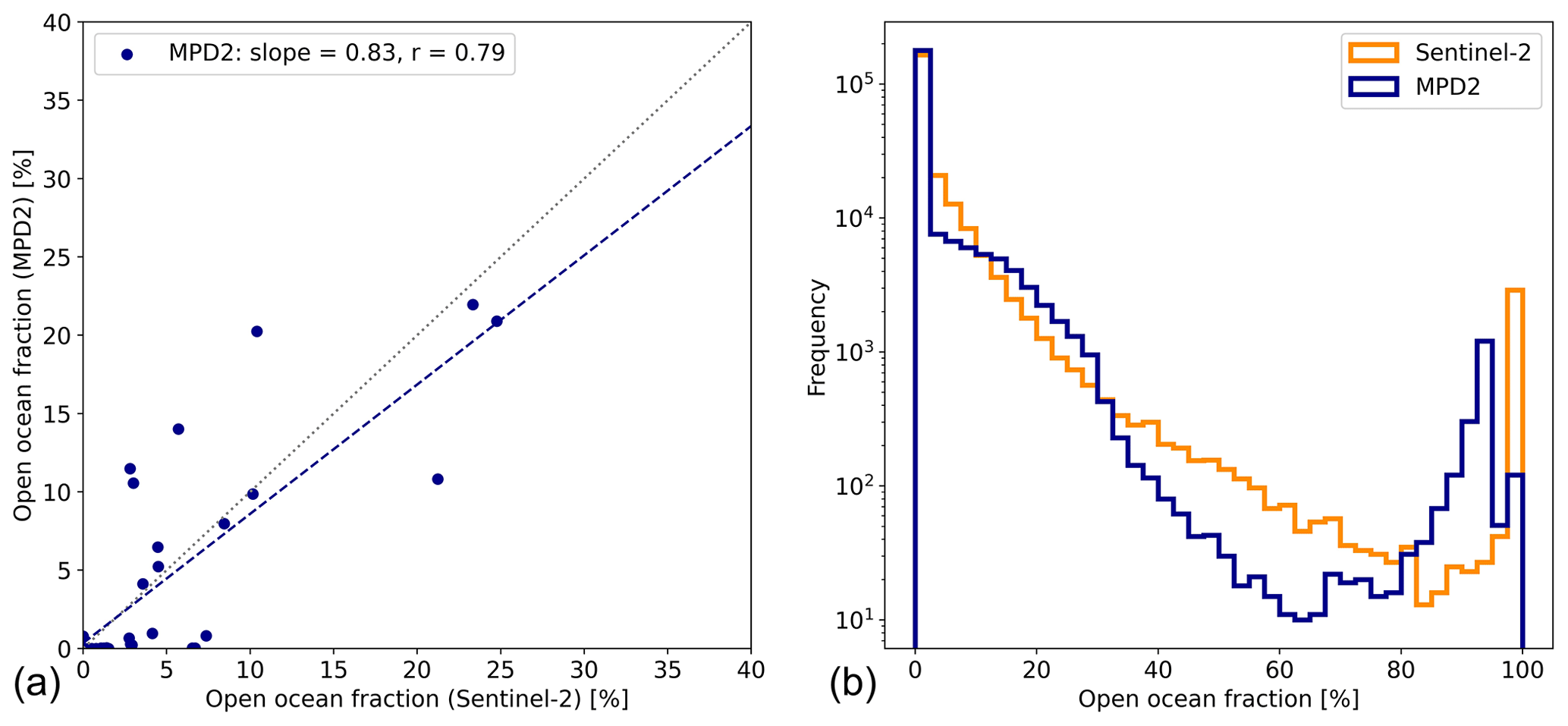
Figure 18(a) Scatter plot of open-ocean fraction soc derived with MPD2 against the Sentinel-2 reference product, averaged per Sentinel-2 scene. The dashed line shows a linear fit to the data points. As a measure of quality, the slope and the correlation coefficient r are specified. (b) Histograms of pixel-wise soc by Sentinel-2 (orange) and MPD2 (dark blue). Note the logarithmic scale of the y axis.
The fraction of open ocean soc newly retrieved with MPD2 is compared to the Sentinel-2 reference data in Fig. 18. The scatter plot (Fig. 18 left) of soc shows a broader scattering than for fmp, demonstrating the difficulties of detecting open ocean due to its spectral neutrality in the visible and NIR range. Especially very small fractions <10 % are often not detected at all. This is most likely because there are not many cases with large open-ocean areas such as polynyas but rather small leads and broken floes beyond the spatial resolution of the MPD. However, the slope of the linear regression is 0.83 and the correlation coefficient 0.79, showing reasonable agreement of the newly retrieved and the reference soc. The histogram of the pixel-wise comparison of the same data in the right panel of Fig. 18 shows that the agreement is almost perfect when there is no open ocean at all in the pixel. That is the case MPD1 was originally developed for. Once there is a small amount of open ocean within the pixel, MPD2 underestimates soc in comparison to the Sentinel-2 reference. The strongest differences occur above open-ocean fractions of 40 %. Up to 80 % soc, MPD2 underestimates and then up to 95 % overestimates soc. The latter is likely because dark melt ponds (with very thin ice below) are being misclassified by the MPD2 algorithm because they already look almost like open ocean. Overall the uncertainty of the open-ocean product is estimated to be 9.1 % (RMSD) with a bias of −0.8.
6.3 Arctic-wide application of MPD2
Figure 19 shows an example of daily Arctic-wide maps of fmp (left), soc (middle), and surface albedo produced with the new MPD2 algorithm from Sentinel-3 data. The swath-wise processed data are gridded into a polar stereographic grid (NSIDC grid) of 6.25 km resolution. In the course of this, the data are averaged daily, discarding grid cells containing fewer than 10 data points or exceeding a standard deviation of the averaged values of 15 %. The broadband albedo displayed in the right panel of Fig. 19 is derived from the retrieved spectral albedo with the spectral-to-broadband conversion developed by Pohl et al. (2020).
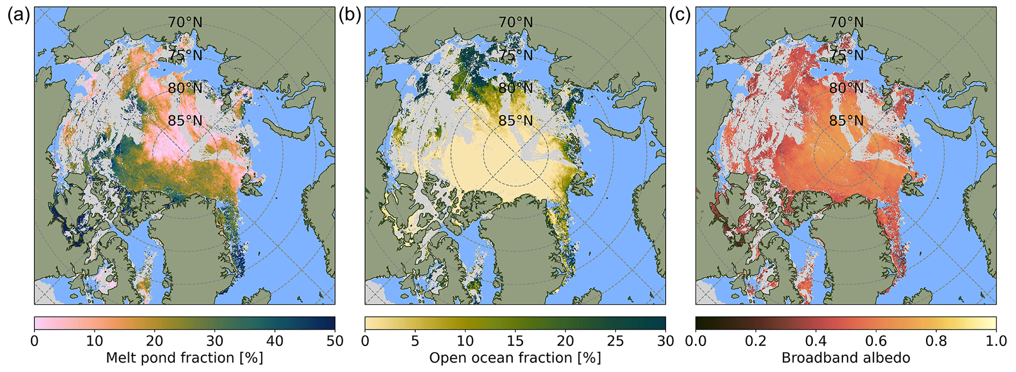
Figure 19Pan-Arctic maps of melt pond fraction fmp (a), open-ocean fraction soc (b), and broadband albedo (c) derived with MPD2 on 30 June 2020. The light blue color indicates open ocean where the retrieval has not been applied. Data gaps due to cloud contamination are gray.
At the end of June, the melt season has already advanced. Especially on the level landfast ice between the islands of the Canadian Archipelago, melt pond fractions higher than 50 % are observed, which is in agreement with in situ and higher-resolution satellite observations from previous years (Landy et al., 2014; Li et al., 2020). Even at latitudes above 80°, melt pond fractions of around 20 % are observed. This is not unusual for this time of the year as shown by results from the MOSAiC campaign in the same summer (Webster et al., 2022). The open-ocean fraction is very low in the central Arctic, but closer to the sea ice edge, soc reaches values beyond 20 %, indicating the break-up of ice floes with a heterogeneous mixture of sea ice, melt ponds, and open ocean as the result. Thus, the broadband albedo is still quite high in the central Arctic, while it is already significantly reduced in the Fram Strait, Kara Sea, Laptev Sea, and Canadian Arctic Archipelago.
This study presents the approach of the new MPD2 algorithm to retrieve melt pond (fmp) and open-ocean (soc) fractions as well as the spectral and broadband albedo of sea ice from top-of-the-atmosphere (TOA) reflectances in the optical and near-infrared (NIR) range measured by satellite. This algorithm builds on the MPD1 algorithm developed by Zege et al. (2015) using the forward model by Malinka et al. (2016, 2018) to find an analytical solution for the bidirectional reflection at the sea ice surface. The novelty of the presented MPD2 algorithm is the introduction of the additional surface type class: open ocean. As shown in Istomina et al. (2023), moderate-resolution spectroradiometers need additional data to retrieve three surface type classes as just TOA reflectances are not sufficient. To afford this, we have improved on the initialization of the optimized state vector X describing the surface, thereby minimizing the risk of running into unreasonable local minima. The 2 m air temperatures from ERA5 are used to calculate a temperature index along the drift track of the sea ice, which is tracked with OSI SAF sea ice drift data (OSI SAF, 2010). With this temperature index we account for regional and seasonal changes, relating to the physical properties of the sea ice surface. In this way the effective grain size aeff and the optical thickness τwi of the ice surface layer are constrained. Without such constraints the spectral unmixing on sub-pixel satellite scale of the three surface types – ice, melt ponds, and open ocean – is not reliably possible. Additionally, we make use of the different spectral behavior of these three surface types (Tschudi et al., 2008; Rösel et al., 2012; Istomina et al., 2015a; Light et al., 2022) to initialize and constrain their area fractions. In fact, a first-order empirical retrieval of fmp and soc from TOA reflectances in the range 400 to 900 nm has been developed and is implemented as an initial guess for the physical forward model.
By using the previously constructed temperature index, seasonal and regional differences of the sea ice optical properties defining its spectral behavior are taken into account. With these improvements, the uncertainty of fmp could be reduced from 12.9 % (MPD1) to 7.8 %, while the uncertainty of soc is estimated to be 9 %. Furthermore, the bias of overestimating fmp has been significantly reduced to +1.7, and the coefficient of determination compared to the reference Sentinel-2 dataset has been increased from 0.39 to 0.89. This is comparable to uncertainties of other melt pond fraction retrievals, e.g., by Rösel et al. (2012) and Ding et al. (2020), and lower than the overestimation bias previously reported (Wright and Polashenski, 2020). While other pan-Arctic melt pond fraction retrievals use artificial neural networks, we have presented a fully physical algorithm to detect melt ponds on sea ice and additionally the fraction of open ocean in the Arctic summer. The longer time series of melt pond and open-ocean fractions from Sentinel-3 satellite data processed with MPD2 will be made available as NetCDF files via https://seaice.uni-bremen.de/ (last access: 14 December 2023). In the future, it is also possible to apply the algorithm to ENVISAT data and thereby extend the time series back to 2002. This can be very useful for, e.g., the study of the sea ice energy budget (Perovich et al., 2002; Nicolaus et al., 2012; Katlein et al., 2021) in the summer period. Thus it provides great potential to improve global climate models (Hunke et al., 2013; Dorn et al., 2018) and better understand climate changes in the Arctic.
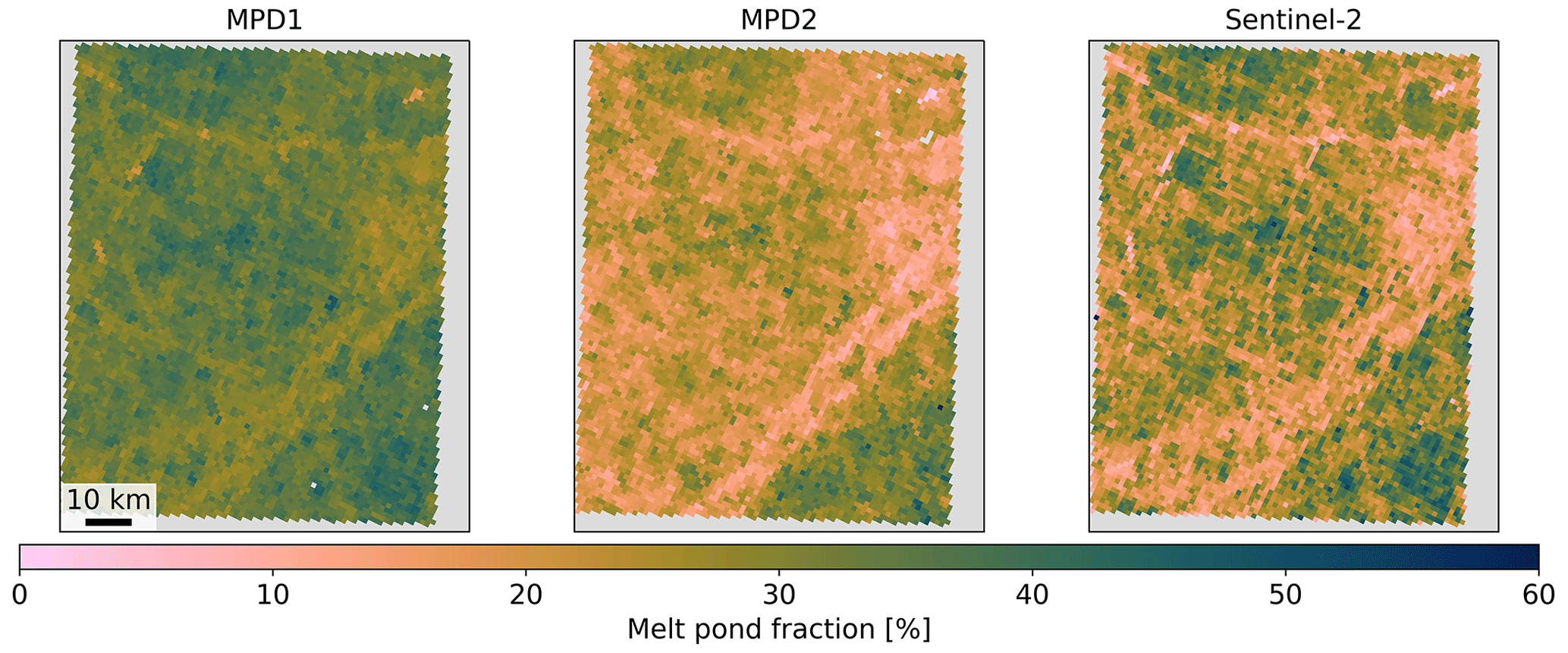
Figure A1Same as Fig. 15 but for an example from 5 July 2018 at approximately 80° N and 109° W. All maps share the same scale and color map.
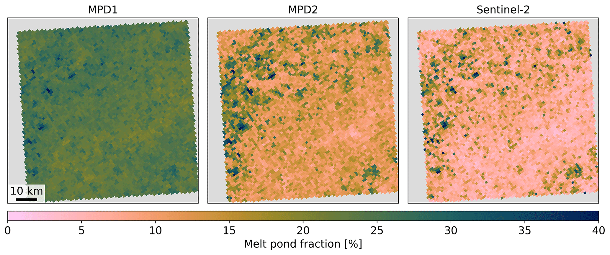
Figure A2Same as Fig. 15 but for an example from 3 July 2017 at approximately 79° N and 120° W. All maps share the same scale and color map.
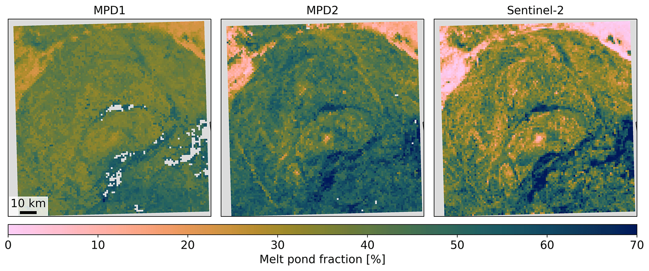
Figure A3Same as Fig. 15 but for an example from 31 May 2021 at approximately 74° N and 133° O. All maps share the same scale and color map.
The Sentinel-3 satellite data used are publicly available at https://ladsweb.modaps.eosdis.nasa.gov/archive/allData/450/ (NASA, 2023).
The Sentinel-2 melt pond fraction product is available via PANGAEA: https://doi.org/10.1594/PANGAEA.950885 (Niehaus and Spreen, 2022).
ERA5 data are made available by the Copernicus Climate Change Service (C3S) at https://cds.climate.copernicus.eu/cdsapp#!/dataset/reanalysis-era5-single-levels?tab=form (Hersbach et al., 2020).
The OSI-405-c sea ice drift data are available via https://thredds.met.no/thredds/catalog/osisaf/met.no/ice/drift_lr/merged/catalog.html (Lavergne et al., 2010).
The spectral albedo data used are publicly available via PANGAEA and data.meereisportal.de and can be retrieved at the following list of links. TARA albedo measurements: https://doi.org/10.1594/PANGAEA.945286 (Nicolaus and Gerland, 2022). Spectral albedo during Alert MAPLI18 measurement campaign: https://doi.pangaea.de/10.1594/PANGAEA.949614 (Nicolau et al., 2024a). Spectral albedo from PS106-ARK31/1 expedition: https://doi.org/10.1594/PANGAEA.875638 (Nicolaus et al., 2017a) and https://doi.org/10.1594/PANGAEA.875652 (Nicolaus et al., 2017b). Albedo measurements from the MOSAiC campaign for the different stations: https://doi.pangaea.de/10.1594/PANGAEA.948876 (Nicolaus et al., 2024b), https://doi.pangaea.de/10.1594/PANGAEA.948828 (Nicolaus et al., 2024c), https://doi.pangaea.de/10.1594/PANGAEA.948712 (Nicolaus et al., 2024d), https://doi.pangaea.de/10.1594/PANGAEA.948572 (Nicolaus et al., 2024e).
HN developed the MPD2 retrieval and the concept of the study, analyzed the data, and wrote the paper. LI, GS, and MN participated in active discussions of the results. LI and AM provided information about the MPD1 version of the algorithm. All authors provided critical feedback on the paper and contributed to the text.
The contact author has declared that none of the authors has any competing interests.
Publisher's note: Copernicus Publications remains neutral with regard to jurisdictional claims made in the text, published maps, institutional affiliations, or any other geographical representation in this paper. While Copernicus Publications makes every effort to include appropriate place names, the final responsibility lies with the authors.
We gratefully acknowledge the funding by the Deutsche Forschungsgemeinschaft (DFG, German Research Foundation) through the Transregional Collaborative Research Centre TRR-172 “ArctiC Amplification: Climate Relevant Atmospheric and SurfaCe Processes, and Feedback Mechanisms (AC)3” (grant 268020496) and the European Union's Horizon 2020 project CRiceS (grant 101003826). Larysa Istomina was funded through the EU Horizon 2020 project SPICES (grant 640161), the project REASSESS (grant 424326801), and the DFG SPP 1158 “Antarctic Research” project. Marcel Nicolaus was partly funded through the EU Horizon 2020 project Arctic Passion (grant 101003472). Some of the data used in this article were produced as part of the international MOSAiC project with the tag MOSAiC20192020 and the following project ID: AWI_PS122_00. We thank all people involved in the expedition of the R/V Polarstern during MOSAiC in 2019–2020 as listed in Nixdorf et al. (2021).
This research has been supported by the Deutsche Forschungsgemeinschaft (grant nos. 268020496 and 424326801) and Horizon 2020 (grant nos. 101003826, 640161, and 101003472).
The article processing charges for this open-access publication were covered by the University of Bremen.
This paper was edited by John Yackel and reviewed by two anonymous referees.
Blackford, J. R.: Sintering and microstructure of ice: a review, J. Phys. D, 40, R355, https://doi.org/10.1088/0022-3727/40/21/R02, 2007. a
Curry, J., Schramm, J., and Ebert, E.: Sea Ice-Albedo Climate Feedback Mechanism, J. Climate, 8, 240–247, 1995. a
Ding, Y., Cheng, X., Liu, J., Hui, F., Wang, Z., and Chen, S.: Retrieval of melt pond fraction over Arctic sea ice during 2000–2019 using an ensemble-based deep neural network, Remote Sens., 12, 2746, https://doi.org/10.3390/RS12172746, 2020. a, b, c, d
Dorn, W., Rinke, A., Köberle, C., Dethloff, K., and Gerdes, R.: HIRHAM–NAOSIM 2.0: The upgraded version of the coupled regional atmosphere-ocean-sea ice model for Arctic climate studies, Geosci. Model Dev. Discuss. [preprint], https://doi.org/10.5194/gmd-2018-278, 2018. a, b
Eicken, H., Grenfell, T. C., Perovich, D. K., Richter-Menge, J. A., and Frey, K.: Hydraulic controls of summer Arctic pack ice albedo, J. Geophys. Res.-Oceans, 109, C08007, https://doi.org/10.1029/2003JC001989, 2004. a, b
Feng, J., Zhang, Y., Cheng, Q., and Tsou, J. Y.: Pan-Arctic melt pond fraction trend, variability, and contribution to sea ice changes, Global Planet. Change, 217, 103932, https://doi.org/10.1016/j.gloplacha.2022.103932, 2022. a, b
Fetterer, F. and Untersteiner, N.: Observations of melt ponds on Arctic sea ice, J. Geophys. Res.-Oceans, 103, 24821–24835, 1998. a
Flocco, D. and Feltham, D. L.: A continuum model of melt pond evolution on Arctic sea ice, J. Geophys. Res.-Oceans, 112, C08016, https://doi.org/10.1029/2006JC003836, 2007. a
Frey, K. E., Perovich, D. K., and Light, B.: The spatial distribution of solar radiation under a melting Arctic sea ice cover, Geophys. Res. Lett., 38, L22501, https://doi.org/10.1029/2011GL049421, 2011. a
Grenfell, T. C. and Maykut, G. A.: The optical properties of ice and snow in the Arctic Basin, J. Glaciol., 18, 445–463, 1977. a
Hersbach, H., Bell, B., Berrisford, P., Hirahara, S., Horányi, A., Muñoz-Sabater, J., Nicolas, J., Peubey, C., Radu, R., Schepers, D., Simmons, A., Soci, C., Abdalla, S., Abellan, X., Balsamo, G., Bechtold, P., Biavati, G., Bidlot, J., Bonavita, M., De Chiara, G., Dahlgren, P., Dee, D., Diamantakis, M., Dragani, R., Flemming, J., Forbes, R., Fuentes, M., Geer, A., Haimberger, L., Healy, S., Hogan, R. J., Hólm, E., Janisková, M., Keeley, S., Laloyaux, P., Lopez, P., Lupu, C., Radnoti, G., de Rosnay, P., Rozum, I., Vamborg, F., Villaume, S., and Thépaut, J.-N.: The ERA5 global reanalysis, Q. J. Roy. Meteor. Soc., 146, 1999–2049, 2020. a, b
Hunke, E. C., Hebert, D. A., and Lecomte, O.: Level-ice melt ponds in the Los Alamos sea ice model, CICE, Ocean Model., 71, 26–42, https://doi.org/10.1016/j.ocemod.2012.11.008, 2013. a, b
Istomina, L. G., von Hoyningen-Huene, W., Kokhanovsky, A. A., and Burrows, J. P.: The detection of cloud-free snow-covered areas using AATSR measurements, Atmos. Meas. Tech., 3, 1005–1017, https://doi.org/10.5194/amt-3-1005-2010, 2010. a
Istomina, L. G., von Hoyningen-Huene, W., Kokhanovsky, A. A., Schultz, E., and Burrows, J. P.: Remote sensing of aerosols over snow using infrared AATSR observations, Atmos. Meas. Tech., 4, 1133–1145, https://doi.org/10.5194/amt-4-1133-2011, 2011. a
Istomina, L., Nicolaus, M., and Perovich, D. K.: Spectral albedo of sea ice and melt ponds measured during POLARSTERN cruise ARK-XXVII/3 (IceArc) in 2012, PANGAEA [data set], https://doi.org/10.1594/PANGAEA.815111, 2013. a
Istomina, L., Heygster, G., Huntemann, M., Marks, H., Melsheimer, C., Zege, E., Malinka, A., Prikhach, A., and Katsev, I.: Melt pond fraction and spectral sea ice albedo retrieval from MERIS data – Part 2: Case studies and trends of sea ice albedo and melt ponds in the Arctic for years 2002–2011, The Cryosphere, 9, 1567–1578, https://doi.org/10.5194/tc-9-1567-2015, 2015a. a, b, c, d, e, f, g
Istomina, L., Heygster, G., Huntemann, M., Schwarz, P., Birnbaum, G., Scharien, R., Polashenski, C., Perovich, D., Zege, E., Malinka, A., Prikhach, A., and Katsev, I.: Melt pond fraction and spectral sea ice albedo retrieval from MERIS data – Part 1: Validation against in situ, aerial, and ship cruise data, The Cryosphere, 9, 1551–1566, https://doi.org/10.5194/tc-9-1551-2015, 2015b. a, b
Istomina, L., Niehaus, H., and Spreen, G.: Updated Arctic melt pond fraction dataset and trends 2002–2023 using ENVISAT and Sentinel-3 remote sensing data, The Cryosphere Discuss. [preprint], https://doi.org/10.5194/tc-2023-142, in review, 2023. a, b, c, d, e, f, g, h
Jäkel, E., Carlsen, T., Ehrlich, A., Wendisch, M., Schäfer, M., Rosenburg, S., Nakoudi, K., Zanatta, M., Birnbaum, G., Helm, V., Herber, A., Istomina, L., Mei, L., and Rohde, A.: Measurements and Modeling of Optical-Equivalent Snow Grain Sizes under Arctic Low-Sun Conditions, Remote Sens., 13, 4904, https://doi.org/10.3390/rs13234904, 2021. a, b
Katlein, C., Arndt, S., Belter, H. J., Castellani, G., and Nicolaus, M.: Seasonal evolution of light transmission distributions through Arctic sea ice, J. Geophys. Res.-Oceans, 124, 5418–5435, 2019. a
Katlein, C., Valcic, L., Lambert-Girard, S., and Hoppmann, M.: New insights into radiative transfer within sea ice derived from autonomous optical propagation measurements, The Cryosphere, 15, 183–198, https://doi.org/10.5194/tc-15-183-2021, 2021. a
Landy, J., Ehn, J., Shields, M., and Barber, D.: Surface and melt pond evolution on landfast first-year sea ice in the Canadian Arctic Archipelago, J. Geophys. Res.-Oceans, 119, 3054–3075, https://doi.org/10.1002/2013JC009617, 2014. a
Lavergne, T., Eastwood, S., Teffah, Z., Schyberg, H., and Breivik, L.-A.: Sea ice motion from low-resolution satellite sensors: An alternative method and its validation in the Arctic, J. Geophys. Res.-Oceans, 115, C10032, https://doi.org/10.1029/2009JC005958, 2010. a
Lee, S., Stroeve, J., Tsamados, M., and Khan, A. L.: Machine learning approaches to retrieve pan-Arctic melt ponds from visible satellite imagery, Remote Sens. Environ., 247, 111919, https://doi.org/10.1016/j.rse.2020.111919, 2020. a, b, c, d
Li, Q., Zhou, C., Zheng, L., Liu, T., and Yang, X.: Monitoring evolution of melt ponds on first-year and multiyear sea ice in the Canadian Arctic Archipelago with optical satellite data, Ann. Glaciol., 61, 154–163, 2020. a
Light, B., Perovich, D. K., Webster, M. A., Polashenski, C., and Dadic, R.: Optical properties of melting first-year Arctic sea ice, J. Geophys. Res.-Oceans, 120, 7657–7675, https://doi.org/10.1002/2015JC011163, 2015. a
Light, B., Smith, M. M., Perovich, D. K., Webster, M. A., Holland, M. M., Linhardt, F., Raphael, I. A., Clemens-Sewall, D., Macfarlane, A. R., Anhaus, P., and Bailey, D. A.: Arctic sea ice albedo: Spectral composition, spatial heterogeneity, and temporal evolution observed during the MOSAiC drift, Elementa, 10, 000103, https://doi.org/10.1525/elementa.2021.000103, 2022. a, b, c, d, e
Liu, J., Song, M., Horton, R. M., and Hu, Y.: Revisiting the potential of melt pond fraction as a predictor for the seasonal Arctic sea ice extent minimum, Environ. Res. Lett., 10, 054017, https://doi.org/10.1088/1748-9326/10/5/054017, 2015. a
Malinka, A., Zege, E., Heygster, G., and Istomina, L.: Reflective properties of white sea ice and snow, The Cryosphere, 10, 2541–2557, https://doi.org/10.5194/tc-10-2541-2016, 2016. a, b, c, d, e
Malinka, A., Zege, E., Istomina, L., Heygster, G., Spreen, G., Perovich, D., and Polashenski, C.: Reflective properties of melt ponds on sea ice, The Cryosphere, 12, 1921–1937, https://doi.org/10.5194/tc-12-1921-2018, 2018. a, b, c, d, e, f, g
Malinka, A. V.: Light scattering in porous materials: Geometrical optics and stereological approach, J. Quant. Spectrosc. Ra., 141, 14–23, 2014. a, b
Marsh, P.: Grain growth in a wet arctic snow cover, Cold Reg. Sci. Technol., 14, 23–31, 1987. a, b
NASA: Sentinel-3 Satellite Data, https://ladsweb.modaps.eosdis.nasa.gov/archive/allData/450/ (last access: 14 August 2023), 2023. a
Nicodemus, F., Richmond, J. C., Hsia, J. J., Ginsberg, I. W., and Limperis, T. L.: Geometrical considerations and nomenclature for reflectance, US Department of Commerce, National Bureau of Standards Washington, DC, USA, vol. 160, 1977. a
Nicolaus, M. and Gerland, S.: Albedo measurements from Radiation Station 2020R24, PANGAEA, https://doi.org/10.1594/PANGAEA.945270, in: Nicolaus, M; Gerland, S (2022): Spectral radiation fluxes, albedo and transmittance from autonomous measurement from Radiation Station 2007R24 at SV Tara in the Arctic Transpolar Drift in 2007, PANGAEA [data set], https://doi.org/10.1594/PANGAEA.945286, 2022. a, b
Nicolaus, M., Gerland, S., Hudson, S. R., Hanson, S., Haapala, J., and Perovich, D. K.: Seasonality of spectral albedo and transmittance as observed in the Arctic Transpolar Drift in 2007, J. Geophys. Res.-Oceans, 115, C11011, https://doi.org/10.1029/2009JC006074, 2010. a, b, c
Nicolaus, M., Katlein, C., Maslanik, J., and Hendricks, S.: Changes in Arctic sea ice result in increasing light transmittance and absorption, Geophys. Res. Lett., 39, L24501, https://doi.org/10.1029/2012GL053738, 2012. a, b
Nicolaus, M., Hoppmann, M., Arndt, S., Hendricks, S., Katlein, C., König-Langlo, G., Nicolaus, A., Rossmann, L., Schiller, M., Schwegmann, S., Langevin, D., and Bartsch, A.: Snow height and air temperature on sea ice from Snow Buoy measurements, PANGAEA [data set] https://doi.org/10.1594/PANGAEA.875638, 2017a. a
Nicolaus, M., Arndt, S., Hoppmann, M., Krumpen, T., Nicolaus, A., and Bartsch, A.: Sea ice drift, surface temperature, and barometric pressure on sea ice from Surface Velocity Profiler measurements, PANGAEA [data set], https://doi.org/10.1594/PANGAEA.875652, 2017b. a
Nicolaus, M., Perovich, D. K., Spreen, G., Granskog, M. A., von Albedyll, L., Angelopoulos, M., Anhaus, P., Arndt, S., Jakob Belter, H., Bessonov, V., Birnbaum, G., Brauchle, J., Calmer, R., Cardellach, E., Cheng, B., Clemens-Sewall, D., Dadic, R., Damm, E., de Boer, G., Demir, O., Dethloff, K., Divine, D. V., Fong, A. A., Fons, S., Frey, M. M., Fuchs, N., Gabarró, C., Gerland, S., Goessling, H. F., Gradinger, R., Haapala, J., Haas, C., Hamilton, J., Hannula, H. R., Hendricks, S., Herber, A., Heuzé, C., Hoppmann, M., Høyland, K. V., Huntemann, M., Hutchings, J. K., Hwang, B., Itkin, P., Jacobi, H. W., Jaggi, M., Jutila, A., Kaleschke, L., Katlein, C., Kolabutin, N., Krampe, D., Kristensen, S. S., Krumpen, T., Kurtz, N., Lampert, A., Lange, B. A., Lei, R., Light, B., Linhardt, F., Liston, G. E., Loose, B., Macfarlane, A. R., Mahmud, M., Matero, I. O., Maus, S., Morgenstern, A., Naderpour, R., Nandan, V., Niubom, A., Oggier, M., Oppelt, N., Pätzold, F., Perron, C., Petrovsky, T., Pirazzini, R., Polashenski, C., Rabe, B., Raphael, I. A., Regnery, J., Rex, M., Ricker, R., Riemann-Campe, K., Rinke, A., Rohde, J., Salganik, E., Scharien, R. K., Schiller, M., Schneebeli, M., Semmling, M., Shimanchuk, E., Shupe, M. D., Smith, M. M., Smolyanitsky, V., Sokolov, V., Stanton, T., Stroeve, J., Thielke, L., Timofeeva, A., Tonboe, R. T., Tavri, A., Tsamados, M., Wagner, D. N., Watkins, D., Webster, M., and Wendisch, M.: Overview of the MOSAiC expedition: Snow and sea ice, Elementa, 10, 000046, https://doi.org/10.1525/elementa.2021.000046, 2022. a, b
Nicolaus, M., Anhaus, P. and Katlein, C.: Spectral radiation fluxes, albedo and transmittance from autonomous measurement from Radiation Station2018R2, deployed during Alert_MAPLI18, Alfred Wegener Institute, Helmholtz Centre for Polar and Marine Research, Bremerhaven, PANGAEA [data set], https://doi.org/10.1594/PANGAEA.949614, 2024a. a
Nicolaus, M., Belter, H. J., Rohde, J., Hoppmann, M., Tao, R., and Katlein, C.: Spectral radiation fluxes, albedo and transmittance from autonomous measurement from Radiation Station 2019R8, deployed during MOSAiC 2019/20, Alfred Wegener Institute, Helmholtz Centre for Polar and Marine Research, Bremerhaven, PANGAEA [data set], https://doi.org/10.1594/PANGAEA.948876, 2024b. a
Nicolaus, M., Anhaus, P., Hoppmann, M., Tao, R., and Katlein, C.: Spectral radiation fluxes, albedo and transmittance from autonomous measurement from Radiation Station 2020R11, deployed during MOSAiC 2019/20, Alfred Wegener Institute, Helmholtz Centre for Polar and Marine Research, Bremerhaven, PANGAEA [data set], https://doi.org/10.1594/PANGAEA.948828, 2024c. a
Nicolaus, M., Anhaus, P., Hoppmann, M., Tao, R., and Katlein, C.: Spectral radiation fluxes, albedo and transmittance from autonomous measurement from Radiation Station 2020R12, deployed during MOSAiC 2019/20, Alfred Wegener Institute, Helmholtz Centre for Polar and Marine Research, Bremerhaven, PANGAEA [data set], https://doi.org/10.1594/PANGAEA.948712, 2024d. a
Nicolaus, M., Anhaus, P., Hoppmann, M., Tao, R., and Katlein, C.: Spectral radiation fluxes, albedo and transmittance from autonomous measurement from Radiation Station 2020R14, deployed during MOSAiC 2019/20, Alfred Wegener Institute, Helmholtz Centre for Polar and Marine Research, Bremerhaven, PANGAEA [data set], https://doi.org/10.1594/PANGAEA.948572, 2024e. a
Niehaus, H. and Spreen, G.: Melt pond fraction on Arctic sea-ice from Sentinel-2 satellite optical imagery (2017–2021), PANGAEA [data set], https://doi.org/10.1594/PANGAEA.950885, 2022. a, b
Niehaus, H., Spreen, G., Birnbaum, G., Istomina, L., Jäkel, E., Linhardt, F., Neckel, N., Fuchs, N., Nicolaus, M., Sperzel, T., Tao, T., Webster, M., and Wright, N.: Sea Ice Melt Pond Fraction Derived From Sentinel-2 Data: Along the MOSAiC Drift and Arctic-Wide, Geophys. Res. Lett., 50, e2022GL102102, https://doi.org/10.1029/2022GL102102, 2023. a, b
Nixdorf, U., Dethloff, K., Rex, M., Shupe, M., Sommerfeld, A., Perovich, D. K., Nicolaus, M., Heuzé, C., Rabe, B., Loose, B., Damm, E., Gradinger, R., Fong, A., Maslowski, W., Rinke, A., Kwok, R., Spreen, G., Wendisch, M., Herber, A., Hirsekorn, M., Mohaupt, V., Frickenhaus, S., Immerz, A., Weiss-Tuider, K., König, B., Mengedoht, D., Regnery, J., Gerchow, P., Ransby, D., Krumpen, T., Morgenstern, A., Haas, C., Kanzow, T., Rack, F. R., Saitzev, V., Sokolov, V., Makarov, A., Schwarze, S., Wunderlich, T., Wurr, K., and Boetius, A.: MOSAiC Extended Acknowledgement, Zenodo, https://doi.org/10.5281/zenodo.5541624, 2021. a
OSI SAF: OSI SAF Global Low Resolution Sea Ice Drift, OSI-405-c, EUMETSAT SAF on Ocean and Sea Ice [data set], https://doi.org/10.15770/EUM_SAF_OSI_NRT_2007, OSI SAF. a, b
Peng, Z., Ding, Y., Qu, Y., Wang, M., and Li, X.: Generating a Long-Term Spatiotemporally Continuous Melt Pond Fraction Dataset for Arctic Sea Ice Using an Artificial Neural Network and a Statistical-Based Temporal Filter, Remote Sens., 14, 4538, https://doi.org/10.3390/rs14184538, 2022. a, b, c
Perovich, D. K.: The optical properties of young sea ice., Washington University, Dept. Atmospheric Sciences, Sci. Rep., 17, https://erdc-library.erdc.dren.mil/jspui/bitstream/11681/2648/1/CRREL-Mono-96-1.pdf (last access: 25 April 2024), 1979. a
Perovich, D. K., Tucker, W. B., and Ligett, K. A.: Aerial observations of the evolution of ice surface conditions during summer, J. Geophys. Res.-Oceans, 107, SHE 24-1–SHE 24-14, https://doi.org/10.1029/2000jc000449, 2002. a, b, c
Perovich, D. K., Grenfell, T. C., Richter-Menge, J. A., Light, B., Tucker III, W. B., and Eicken, H.: Thin and thinner: Sea ice mass balance measurements during SHEBA, J. Geophys. Res.-Oceans, 108, 8050, https://doi.org/10.1029/2001JC001079, 2003. a
Perovich, D. K., Richter-Menge, J. A., Jones, K. F., and Light, B.: Sunlight, water, and ice: Extreme Arctic sea ice melt during the summer of 2007, Geophys. Res. Lett., 35, L11501, https://doi.org/10.1029/2008GL034007, 2008. a
Pohl, C., Istomina, L., Tietsche, S., Jäkel, E., Stapf, J., Spreen, G., and Heygster, G.: Broadband albedo of Arctic sea ice from MERIS optical data, The Cryosphere, 14, 165–182, https://doi.org/10.5194/tc-14-165-2020, 2020. a, b, c, d
Polashenski, C., Perovich, D., and Courville, Z.: The mechanisms of sea ice melt pond formation and evolution, J. Geophys. Res.-Oceans, 117, C01001, https://doi.org/10.1029/2011JC007231, 2012. a, b
Press, W. H.: Numerical recipes 3rd edition: The art of scientific computing, Cambridge university press, 2007. a, b
Rösel, A. and Kaleschke, L.: Comparison of different retrieval techniques for melt ponds on Arctic sea ice from Landsat and MODIS satellite data, Ann. Glaciol., 52, 185–191, https://doi.org/10.3189/172756411795931606, 2011. a
Rösel, A., Kaleschke, L., and Birnbaum, G.: Melt ponds on Arctic sea ice determined from MODIS satellite data using an artificial neural network, The Cryosphere, 6, 431–446, https://doi.org/10.5194/tc-6-431-2012, 2012. a, b, c, d, e, f, g
Scharien, R. K. and Yackel, J. J.: Analysis of surface roughness and morphology of first-year sea ice melt ponds: Implications for microwave scattering, IEEE T. Geosci. Remote, 43, 2927–2939, 2005. a
Schröder, D., Feltham, D. L., Flocco, D., and Tsamados, M.: September Arctic sea-ice minimum predicted by spring melt-pond fraction, Nat. Clima. Change, 4, 353–357, 2014. a
Screen, J. A.: An ice-free Arctic: what could it mean for European weather?, Weather, 76, 327–328, 2021. a
Serreze, M. C., Barrett, A. P., Stroeve, J. C., Kindig, D. N., and Holland, M. M.: The emergence of surface-based Arctic amplification, The Cryosphere, 3, 11–19, https://doi.org/10.5194/tc-3-11-2009, 2009. a
Stroeve, J. C., Kattsov, V., Barrett, A., Serreze, M., Pavlova, T., Holland, M., and Meier, W. N.: Trends in Arctic sea ice extent from CMIP5, CMIP3 and observations, Geophys. Res. Lett., 39, L16502, https://doi.org/10.1029/2012GL052676, 2012a. a
Stroeve, J. C., Serreze, M. C., Holland, M. M., Kay, J. E., Malanik, J., and Barrett, A. P.: The Arctic's rapidly shrinking sea ice cover: A research synthesis, Climatic Change, 110, 1005–1027, https://doi.org/10.1007/s10584-011-0101-1, 2012b. a
Tao, R., Nicolaus, M., Katlein, C., Philipp, A., Mario, H., Niehaus, H., Jäkel, E., Wendisch, M., and Haas, C.: Seasonality of spectral radiative fluxes and optical properties of Arctic sea ice, Elementa, https://eartharxiv.org/repository/object/6702/download/12951/ (last access: 25 April 2024), 2023. a
Tschudi, M. A., Maslanik, J. A., and Perovich, D. K.: Derivation of melt pond coverage on Arctic sea ice using MODIS observations, Remote Sens. Environ., 112, 2605–2614, 2008. a, b, c, d
Tynes, H., Kattawar, G. W., Zege, E. P., Katsev, I. L., Prikhach, A. S., and Chaikovskaya, L. I.: Monte Carlo and multi-component approximation methods for vector radiative trans- fer by use of effective Mueller matrix calculations, Appl. Optics, 40, 400–412, 2001. a
Wang, M., Su, J., Landy, J., Leppäranta, M., and Guan, L.: A New Algorithm for Sea Ice Melt Pond Fraction Estimation From High-Resolution Optical Satellite Imagery, J. Geophys. Res.-Oceans, 125, 1–14, https://doi.org/10.1029/2019JC015716, 2020. a
Webster, M. A., Holland, M. M., Wright, N., Hendricks, S., Hutter, N., Itkin, P., Light, B., Linhardt, F., Perovich, D. K., Raphael, I. A., Smith, M. M., Von Albedyll, L., and Zhang, J.: Spatiotemporal evolution of melt ponds on Arctic sea ice: MOSAiC observations and model results, Elementa, 10, 000072, https://doi.org/10.1525/elementa.2021.000072, 2022. a, b
Wendisch, M., Brückner, M., Crewell, S., et al.: Atmospheric and surface processes, and feedback mechanisms determining Arctic amplification: A review of first results and prospects of the (AC) 3 project, B. Am. Meteorol. Soc., 104, E208–E242, 2023. a, b
Wright, N. C. and Polashenski, C. M.: How Machine Learning and High-Resolution Imagery Can Improve Melt Pond Retrieval From MODIS Over Current Spectral Unmixing Techniques, J. Geophys. Res.-Oceans, 125, e2019JC015569, https://doi.org/10.1029/2019JC015569, 2020. a
Yackel, J. J., Barber, D. G., and Hanesiak, J. M.: Melt ponds on sea ice in the Canadian Archipelago: 1. Variability in morphological and radiative properties, J. Geophys. Res.-Oceans, 105, 22049–22060, https://doi.org/10.1029/2000jc900075, 2000. a
Zege, E., Malinka, A., Katsev, I., Prikhach, A., Heygster, G., Istomina, L., Birnbaum, G., and Schwarz, P.: Algorithm to retrieve the melt pond fraction and the spectral albedo of Arctic summer ice from satellite optical data, Remote Sens. Environ., 163, 153–164, https://doi.org/10.1016/j.rse.2015.03.012, 2015. a, b, c, d, e, f, g, h, i
Zhang, J., Schweiger, A., Webster, M., Light, B., Steele, M., Ashjian, C., Campbell, R., and Spitz, Y.: Melt pond conditions on declining Arctic sea ice over 1979–2016: Model development, validation, and results, J. Geophys. Res.-Oceans, 123, 7983–8003, 2018. a
- Abstract
- Introduction
- Datasets
- The Melt Pond Detection 2 algorithm
- Initial values for effective grain size aeff and optical thickness τwi
- Initial values for melt pond fmp and open-ocean soc fraction
- Verification and discussion of results
- Conclusions
- Appendix A: Additional figures
- Data availability
- Author contributions
- Competing interests
- Disclaimer
- Acknowledgements
- Financial support
- Review statement
- References