Meteoric water and glacial melt in the southeastern Amundsen Sea: a time series from 1994 to 2020

Ice sheet mass loss from Antarctica is greatest in the Amundsen Sea sector, where “warm” modified Circumpolar Deep Water moves onto the continental shelf and melts and thins the bases of ice shelves hundreds of meters below the sea surface. We use nearly 1000 paired salinity and oxygen isotope analyses of seawater samples collected on seven expeditions from 1994 to 2020 to produce a time series of glacial meltwater inventory for the southeastern Amundsen Sea continental shelf. Deep water column salinity–δ¹⁸O relationships yield freshwater end-member δ¹⁸O values from $-\mathrm{31.3}\pm \mathrm{1.0}\mathrm{‰}$ to $-\mathrm{28.4}\pm \mathrm{1.0}\mathrm{‰}$, consistent with the isotopic composition of local glacial ice. We use a two-component meteoric water end-member approach that accounts for precipitation in the upper water column, and a pure glacial meteoric water end-member is employed for the deep water column. Meteoric water inventories are comprised of nearly pure glacial meltwater in deep shelf waters and of >74 % glacial meltwater in the upper water column. Total meteoric water inventories range from 8.1±0.7 to 9.6±0.8 m and exhibit greater interannual variability than trend over the study period, based on the available data. The relatively long residence time in the southeastern Amundsen Sea allows changes in mean meteoric water inventories to diagnose large changes in local melt rates, and improved understanding of regional circulation could produce well-constrained glacial meltwater fluxes. The two-component meteoric end-member technique improves the accuracy of the sea ice melt and meteoric fractions estimated from seawater δ¹⁸O measurements throughout the entire water column and increases the utility for the broader application of these estimates.

1 Introduction

Four decades of observations show significant and increasing glacial mass loss from Antarctica (Rignot et al., 2011, 2019; Velicogna et al., 2014). The Special Report on the Ocean and Cryosphere in a Changing Climate (SROCC) projected 0.61 to 1.10 m of sea level rise (SLR) by 2100 under RCP8.5 forcing, with uncertainty largely hinging on the future of the Antarctic Ice Sheet (IPCC, 2022). Over the past 2 decades, losses from the West Antarctic Ice Sheet (WAIS) comprised 84±12 % of the total Antarctic contribution to SLR (5.5±2.2 mm from 1993 to 2018; WCRP Global Sea Level Budget Group, 2018), with glaciers flowing into the Amundsen Sea sector (particularly the Pine Island and Thwaites glaciers) dominating the overall negative mass balance of the ice sheet (Rignot et al., 2019; Shepherd et al., 2019).

High ice shelf basal melt rates in the southeastern (SE) Amundsen Sea have been linked to the flow of “warm” and salty modified Circumpolar Deep Water (mCDW) onto the continental shelf, separated by cooler but fresher waters above by a thermocline between 300 and 700 m (Dutrieux et al., 2014; Jacobs et al., 2011). mCDW flows from the continental shelf break towards SE Amundsen Sea ice shelves via “central” and “eastern” glacially carved bathymetric troughs (Nakayama et al., 2013). This warm mCDW penetrates into sub-ice-shelf cavities (Jacobs et al., 1996; Paolo et al., 2015; Pritchard et al., 2012) where it can access ice shelf grounding lines (Rignot and Jacobs, 2002). To access the Pine Island Ice Shelf (PIIS) grounding line, mCDW passes between the bottom of the ice shelf at ∼350 m and a seafloor ridge at ∼700 m (Jenkins et al., 2010). Basal melt is driven by total heat transport, which depends more on the thickness of the mCDW layer transported onshore than its temperature (Dutrieux et al., 2014; Jenkins et al., 2018), with the thickness controlled by local wind forcing of a shelf break undercurrent, in turn influenced by the Amundsen Sea Low. Despite the strong sensitivity of these ice shelves to ocean forcing as well as evidence of increasing mass loss in this region, estimates of Antarctic SLR contributions from basal melt remain poorly constrained (van der Linden et al., 2023).

Southern Ocean water masses have typically been differentiated and defined by measurements of temperature and salinity, and less often by including oxygen isotopes (δ¹⁸O; Jacobs et al., 1985, 2002; Jeon et al., 2021; Meredith et al., 2008, 2010, 2013; Brown et al., 2014; Randall-Goodwin et al., 2015; Silvano et al., 2018; Biddle et al., 2019). Salinity–δ¹⁸O relationships can be used to infer the source and concentration of highly δ¹⁸O-depleted glacial meltwater from seawater properties (Jacobs et al., 1985, 2002; Hellmer et al., 1998; Meredith et al., 2008; Randall-Goodwin et al., 2015). A spatial and temporal array of T, S, and δ¹⁸O can be utilized to track glacial meltwater (GMW) content and distribution, especially in nearshore waters adjacent to melting ice shelves. Prior studies have used δ¹⁸O measurements to estimate meteoric water (precipitation and GMW) abundance in the Amundsen Sea (Biddle et al., 2019; Jeon et al., 2021; Randall-Goodwin et al., 2015) and elsewhere around Antarctica (Meredith et al., 2008, 2010, 2013; Brown et al., 2014; Silvano et al., 2018); however, so far, they have revealed little about temporal variability or possible trends in meteoric water content. Here, we use nearly 1000 seawater isotope samples collected during seven austral summers from 1994 to 2020 (Fig. 1) to investigate meteoric water sources, water column inventories, and their interannual variability in the SE Amundsen Sea.

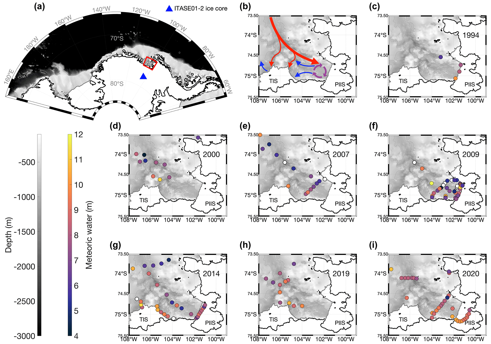
Figure 1 Study area bathymetry, circulation, and δ¹⁸O sampling locations for 7 respective years between 1994 and 2020. The 800 m isobaths are shown as thin gray lines. (a) SE Amundsen Sea study area and the location of the ITASE 01-2 ice core. (b) Location of the Pine Island Bay gyre (purple), pathways of warm deep mCDW (red) toward the ice shelves, and pathways of shallower meltwater-rich waters (blue) from beneath Pine Island Ice Shelf (PIIS) (Nakayama et al., 2019; Wåhlin et al., 2021; Dotto et al., 2022). (c–i) Colored dots show sample locations, with colors representing depth-integrated glacial meltwater inventories between 0 and 800 m from 1994 to 2020. Thick gray lines indicate the seaward boundaries of Thwaites Ice Shelf (TIS) and the PIIS. Calving fronts are referenced to 2000 (Schaffer and Timmermann, 2016; Fretwell et al., 2013), representing a relatively stable location before a ∼20 km retreat following calving events between 2017 and 2020 (Joughin et al., 2021a). Stations where sampling did not extend to the seafloor show only partial water column inventories, and stations shown as white dots (2007, 2009, and 2014) had two or fewer depths sampled. In 2000, 2007, and 2019, access to sampling along the front of the PIIS calving front was precluded by fast ice.

2 Data and methods

2.1 Sample collection and analysis

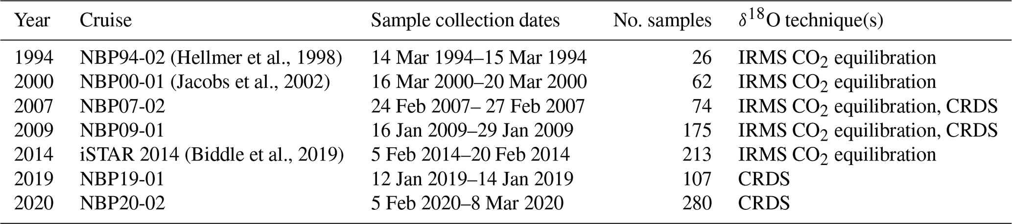
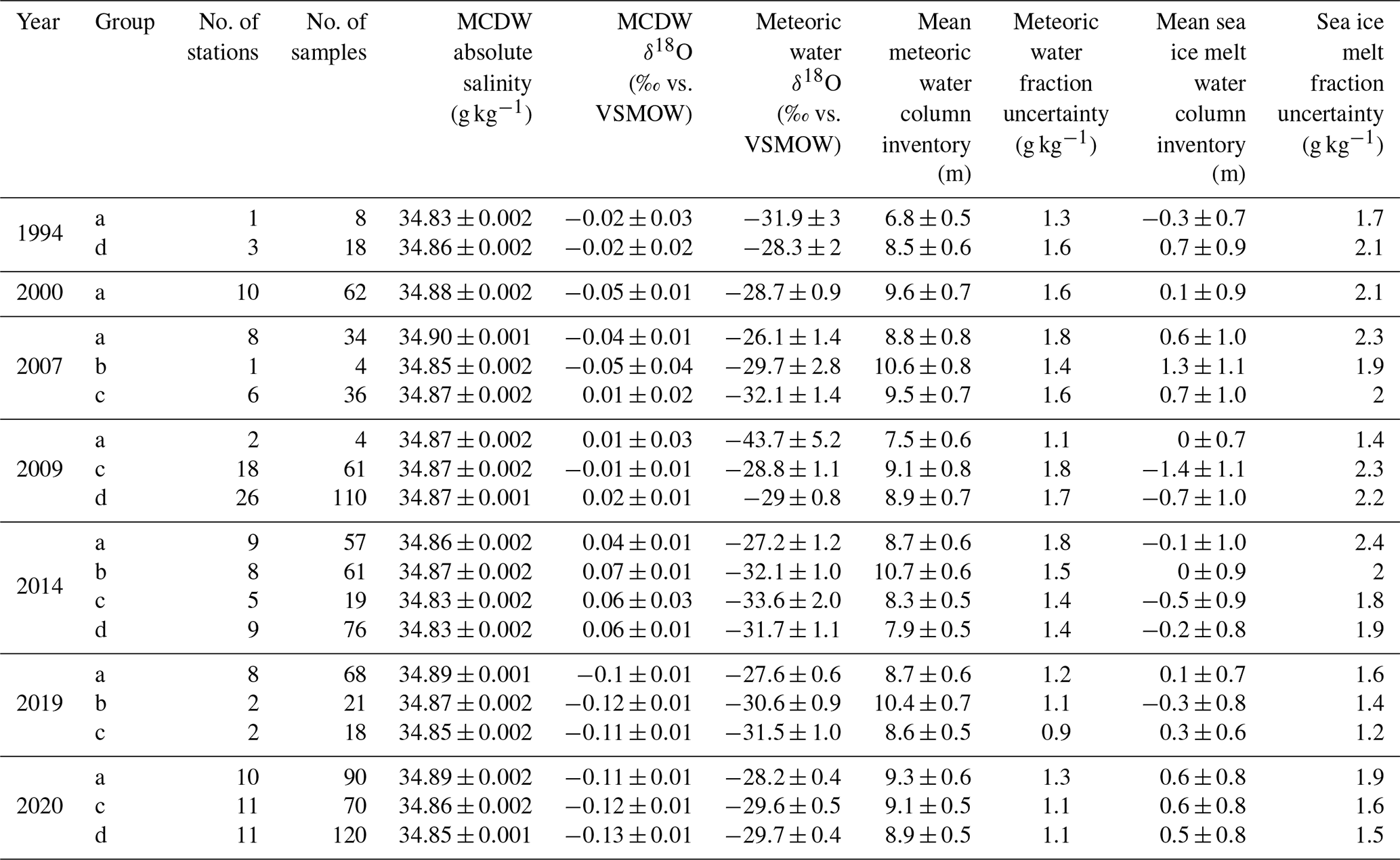
We compile data from samples collected during seven field seasons in the SE Amundsen Sea from 1994 to 2020 (Fig. 1, Table 1). Salinity profiles were obtained using calibrated conductivity cells on SBE 911 conductivity–temperature–depth (CTD) instruments, monitored with shipboard bottle sample analyses using Guildline Autosal and Portasal salinometers calibrated with International Association for the Physical Sciences of the Oceans (IAPSO) seawater salinity standards. δ¹⁸O samples from 2019 and 2020 were collected in glass serum vials capped with rubber stoppers and aluminum seals (Appendix A8), for which internal lab data demonstrate the maintenance of seawater δ¹⁸O sample integrity for 4 or more years. In all other years, samples were collected in bottles with taped (1994, 2000, 2007, and 2009) or PARAFILM-wrapped (2014), threaded caps. The 2009 and 2014 samples were stored for several years before δ¹⁸O analysis.

In 1994, 2000, 2007, 2009, and 2014, δ¹⁸O was measured using an isotope ratio mass spectrometer (IRMS; a Micromass Optima Multiprep or a Finnigan MAT252 HDO). All samples collected in 2019 and 2020 and some samples collected in 2007 and 2009 were measured with a Picarro L2140-i cavity ring-down spectroscopy (CRDS) system. Equivalence has been demonstrated between CRDS and IRMS measurements (Appendix A7; Walker et al., 2016). In all cases, values are reported as per mil (‰) deviations (δ), relative to Vienna Standard Mean Ocean Water (VSMOW2; Coplen, 1994).

Table 1 Summary of δ¹⁸O data sources, sampling intervals, methods, and applications.

Some of the 2009 samples were processed at Rutgers University in 2010 using a Micromass IRMS; the remainder were processed using a Picarro CRDS system at Stanford University in 2020. The latter samples were subject to extensive quality control before being included in this study (Appendix A6). A subset of 100 samples from 2019 and 2020 were processed concurrently using CO₂ equilibration on a Finnigan MAT252 IRMS and CRDS via vaporizer to ensure data comparability between the instruments (Appendix A7). Measurements for all years achieved a precision of 0.04 ‰ for IRMS and 0.02 ‰ for CRDS, based on replicate analyses.

After a review of the literature, we considered a possible salt effect in measured seawater δ¹⁸O, as suggested by a small number of studies (Lécuyer et al., 2009; Skrzypek and Ford, 2014; Benetti et al., 2017). As no salt effect offset was applied to the previously published data in this study (1994, 2000, and 2014), we have not applied any offset to data from other years. The mCDW δ¹⁸O value (Table 2) for 2014 is significantly higher than other years (Appendix A2) – likely due to a calibration offset, although this may also point to sample storage issues. The mCDW and meteoric water end-members are defined from observations each year, minimizing the impact of interlaboratory offsets on the results (Sect. 2.2, Appendix A2).

2.2 Three-end-member mixing model

We adapt an approach from Östlund and Hut (1984) as applied in the Peninsula–Bellingshausen–Amundsen region of West Antarctica (Biddle et al., 2019; Jeon et al., 2021; Randall-Goodwin et al., 2015; Meredith et al., 2008, 2010, 2013) and near the Totten Ice Shelf (Silvano et al., 2018). We use a three-end-member mixing model (Eqs. 1–3) to determine water source fractions in the field area. The model assumes that the observed δ¹⁸O and salinity values result from mixtures of mCDW, sea ice melting/freezing, and meteoric waters contributing a range of δ¹⁸O and salinity signatures. Model outputs (mCDW, meteoric water, and sea ice melt fractions) critically depend on appropriate end-member inputs, which will affect the resulting water source fractions and the interpretation of any changes through time. To minimize issues that could arise from interlaboratory calibration offsets (Sect. 2.1, Appendix A2), we define mCDW and meteoric water end-members separately for each year (Table 2).

Equations (1)–(3) outline the three-end-member mixing model. This model uses the absolute salinity and δ¹⁸O of mCDW, sea ice melt, and meteoric water endpoints to solve for the relative fractions of the three water sources in each sample analyzed.

$$\begin{array}{}\text{(1)}& {\displaystyle }{f}_{\mathrm{sim}}+f_{\mathrm{met}}+f_{\mathrm{mcdw}}=\mathrm{1}\text{(2)}& {\displaystyle }{f}_{\mathrm{sim}}\times S_{\mathrm{sim}}+f_{\mathrm{met}}\times S_{\mathrm{met}}+f_{\mathrm{mcdw}}\times S_{\mathrm{mcdw}}=S_{\mathrm{obs}}\text{(3)}& {\displaystyle }{f}_{\mathrm{sim}}\times {\mathit{\delta }}_{\mathrm{sim}}+f_{\mathrm{met}}\times {\mathit{\delta }}_{\mathrm{met}}+f_{\mathrm{mcdw}}\times {\mathit{\delta }}_{\mathrm{mcdw}}={\mathit{\delta }}_{\mathrm{obs}}\end{array}$$

In the above expressions, f is the fraction of the water source, S is salinity, δ represents δ¹⁸O, “sim” is sea ice melt, “met” is meteoric water, “mcdw” is modified Circumpolar Deep Water, and “obs” represents the observed sample.

The mCDW is the warmest, saltiest, and least δ¹⁸O-depleted water mass in the region, and it comprises the vast majority of the overall water column. Interannual changes in mCDW inflow will result from variable wind forcing (Dotto et al., 2019; Holland et al., 2019; Kim et al., 2021), combined with on-shelf lateral and vertical mixing. In the three-end-member mixing model, mCDW is defined by the mixing line of data >200 m, with mCDW being the δ¹⁸O value at the salinity maximum (Biddle et al., 2017) (Fig. 2, Sect. 3.1, Appendix A1). Sea ice end-member isotopic values adopted from previous studies in the Amundsen and Bellingshausen region (Meredith et al., 2008, 2010, 2013; Randall-Goodwin et al., 2015; Biddle et al., 2019) are based on the δ¹⁸O of surface water with an offset to account for isotopic fractionation due to freezing (Melling and Moore, 1995; Rohling, 2013).

The greatest end-member uncertainty is associated with the meteoric water end-member, which can include basal melt, local and imported iceberg melt, and local and nonlocal precipitation. Meteoric waters >200 m will consist almost entirely of GMW (Jenkins, 1999; Randall-Goodwin et al., 2015; Biddle et al., 2019) and can be fingerprinted using the zero-salinity intercept of linear regressions through salinity–δ¹⁸O data, as shown in Fig. 2 (Fairbanks, 1982; Paren and Potter, 1984; Potter et al., 1984; Jacobs et al., 1985; Hellmer et al., 1998; Jenkins, 1999; Meredith et al., 2008) (Sect. 3.1). Even meteoric water in the upper 200 m will consist primarily of GMW (Meredith et al., 2008; Bett et al., 2020); however, it is also likely to contain some fraction of precipitation with a less negative δ¹⁸O value.

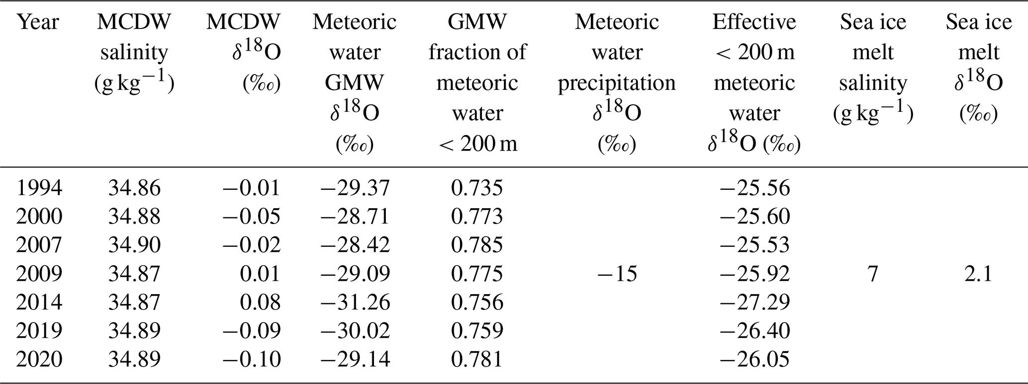
The Pine Island–Thwaites area receives ∼0.5 m yr⁻¹ (water equivalent) of precipitation (Boisvert et al., 2020; Donat-Magnin et al., 2021). Local precipitation collected in 2019 at 72.5^∘ S had a δ¹⁸O value of −15 ‰, consistent with studies of precipitation at this latitude and elevation (Masson-Delmotte et al., 2008). To calculate the most accurate meteoric water and sea ice melt fractions, we account for the presence of precipitation in the upper water column. With 2 full years' worth of precipitation (residence time of local deep shelf waters ∼2 years; Tamsitt et al., 2021) in the upper water column, those meteoric waters must be comprised of >74 % GMW (Appendix A4). We use a two-component meteoric water end-member approach, with a “pure” GMW end-member, as calculated from the linear regression through those δ¹⁸O and salinity data (Fig. 2, Table 2, Sect. 3.1), used in the deep water column and an end-member comprised of precipitation and GMW (Table 2) used in the upper water column.

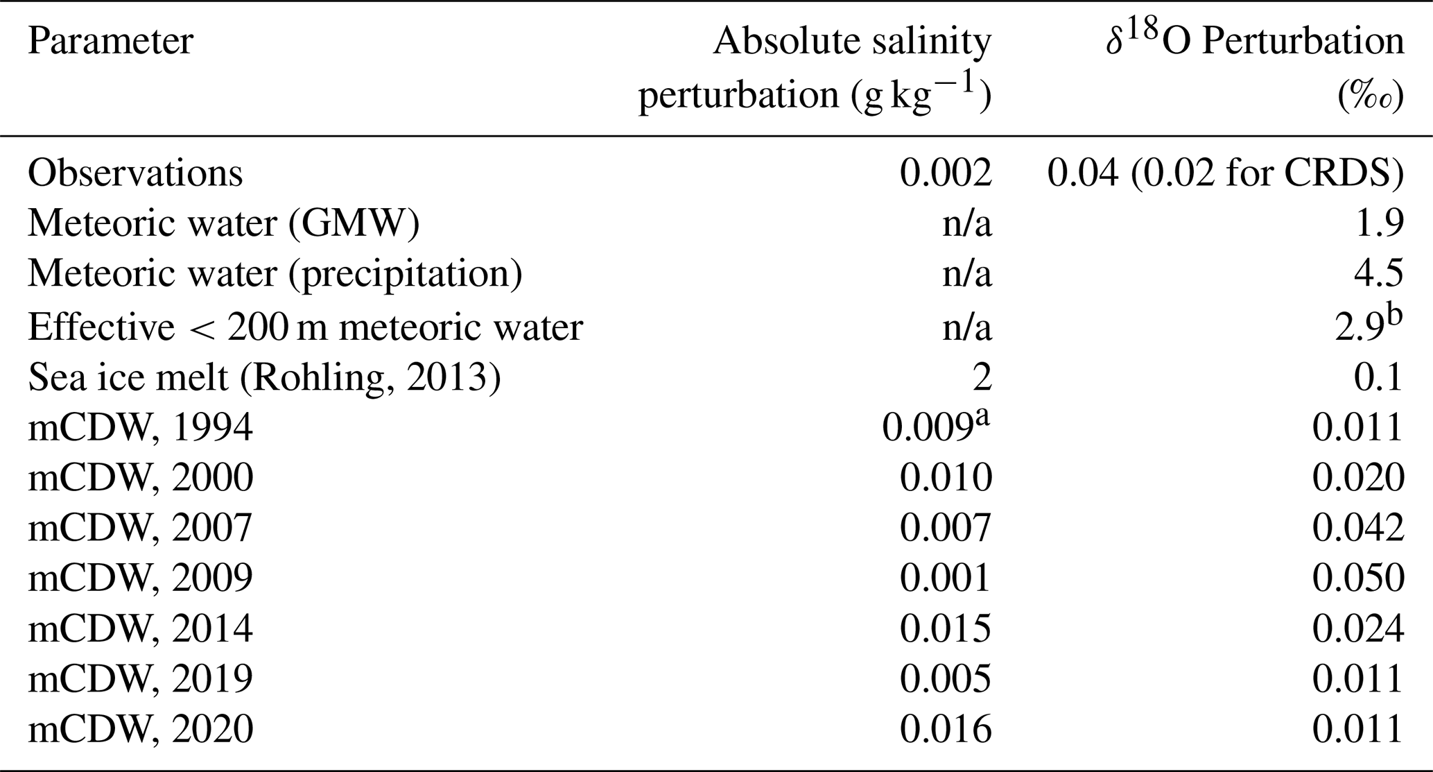
Table 2 Base salinity and δ¹⁸O values used in the three-end-member mixing model. mCDW and meteoric GMW components are defined independently using the mCDW–GMW mixing line produced from (>200 m depth) salinity and δ¹⁸O observations for each year, as the salinity maximum and zero-salinity intercept, respectively (Fig. 2, Sect. 3.1, Appendix A1). In the upper 200 m, a meteoric end-member comprised of a weighted average between precipitation and the GMW fraction is used (Appendix A4). Sea ice melt uses the same values for each year. Salinities are reported as absolute salinity (g kg⁻¹).

3 Results

3.1 Meteoric waters defined by the δ¹⁸O–salinity relationship

Freshwater end-members (zero-salinity δ¹⁸O intercepts) over the seven sampled summers differ by <3 ‰, ranging from $-\mathrm{28.4}\pm \mathrm{1.0}\mathrm{‰}$ to $-\mathrm{31.3}\pm \mathrm{1.0}\mathrm{‰}$ with a standard deviation of 1.0 ‰ across years (Fig. 2, Table 2). These measurements are consistent with the nearest ice core (ITASE 01-2, from 77.84^∘ S, 102.91^∘ W; Fig. 1a; Schneider et al., 2006; Steig et al., 2005) with a mass-averaged δ¹⁸O value of $-\mathrm{29.8}\pm \mathrm{1.9}\mathrm{‰}$. Ice cores further east have less-negative δ¹⁸O values ($\sim -\mathrm{20}\mathrm{‰}$; Thomas et al., 2009), whereas those further west are more negative ($\sim -\mathrm{40}\mathrm{‰}$; Blunier and Brook, 2001). Intercept standard error ranges from ±0.3 ‰ in 2020 to ±1.9 ‰ in 2009. End-member extrapolations from the regional salinity and δ¹⁸O measurements indicate that freshwater introduced to the water column is dominated by locally derived GMW, as intimated earlier from 1994 data (Hellmer et al., 1998). While winter water, produced during sea ice formation, also has a depleted δ¹⁸O signature, these waters are less depleted than those influenced by GMW (Jenkins, 1999). Aggressively removing winter water samples ($\mathrm{\Theta }<-\mathrm{1.5}$ ^∘C) from the regression had no impact on the zero-salinity intercepts. The calculated intercepts were also unaffected by using only those data falling directly on the mCDW–GMW mixing line in T–S space (distinct from the mCDW–winter water mixing line).

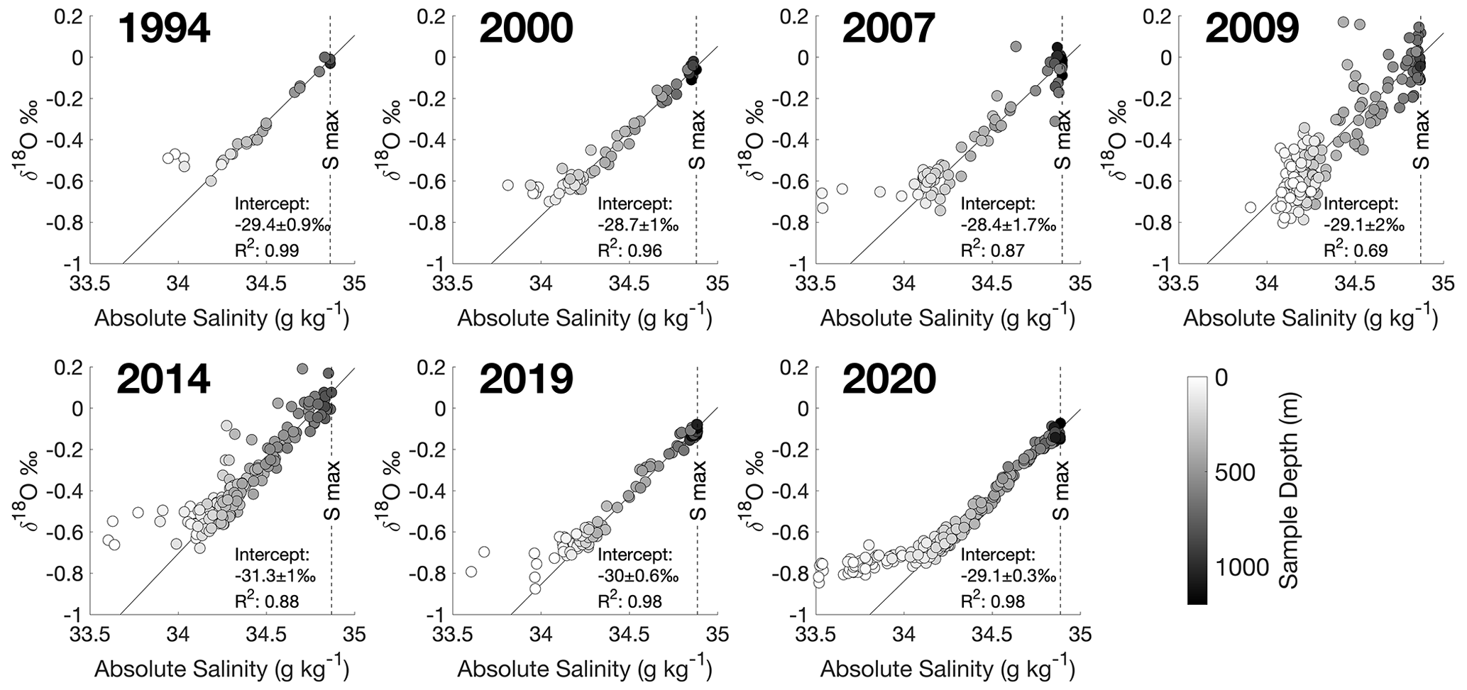
Figure 2 Salinity vs. δ¹⁸O plots for each year, shaded by depth. Linear regressions (solid gray lines, with R² from 0.69 in 2009 to 0.99 in 1994) project to zero-salinity glacial meltwater end-member intercepts using data >200 m. Dashed vertical lines indicate the mCDW salinity maxima (Table 2). Data diverge from the mCDW–meteoric water mixing line in the upper water column, where sea ice melt freshens the resultant mixture but has an enriching effect on δ¹⁸O (Table 2). Years with greater divergence at the surface have more sea ice melt (Fig. 4). The most negative upper water column seawater δ¹⁸O measurements tend to reach minima between −0.9 ‰ and −0.6 ‰. Intercept uncertainty is the standard error of the linear regression intercept through data >200 m.

Samples below 200 m show a strong δ¹⁸O–salinity relationship, forming a mixing line between mCDW and a (glacial) meteoric freshwater end-member introduced at depth. Closer to the surface (from 10 m in 2009 to 160 m in 2000), data diverge from the mixing line due to the net influence of sea ice melt and local precipitation, moving the δ¹⁸O of the mixture in a more positive direction. Below 200 m, the δ¹⁸O–salinity relationship is strongly linear in all years, with 1994, 2000, 2019, and 2020 showing the strongest fit.

3.2 Vertical distribution of meteoric water illustrates basal melt

A three-end-member mixing model of mCDW, sea ice melt, and meteoric water is used to determine the constituent freshwater components of seawater (Eqs. 1–3) at all depths sampled in the water column (Fig. 3). We minimize the potential impact of analytical calibration offsets between laboratories on calculated meteoric water fractions by calculating mCDW and meteoric water end-members from each year’s data individually (Sect. 2.1, Appendix A2).

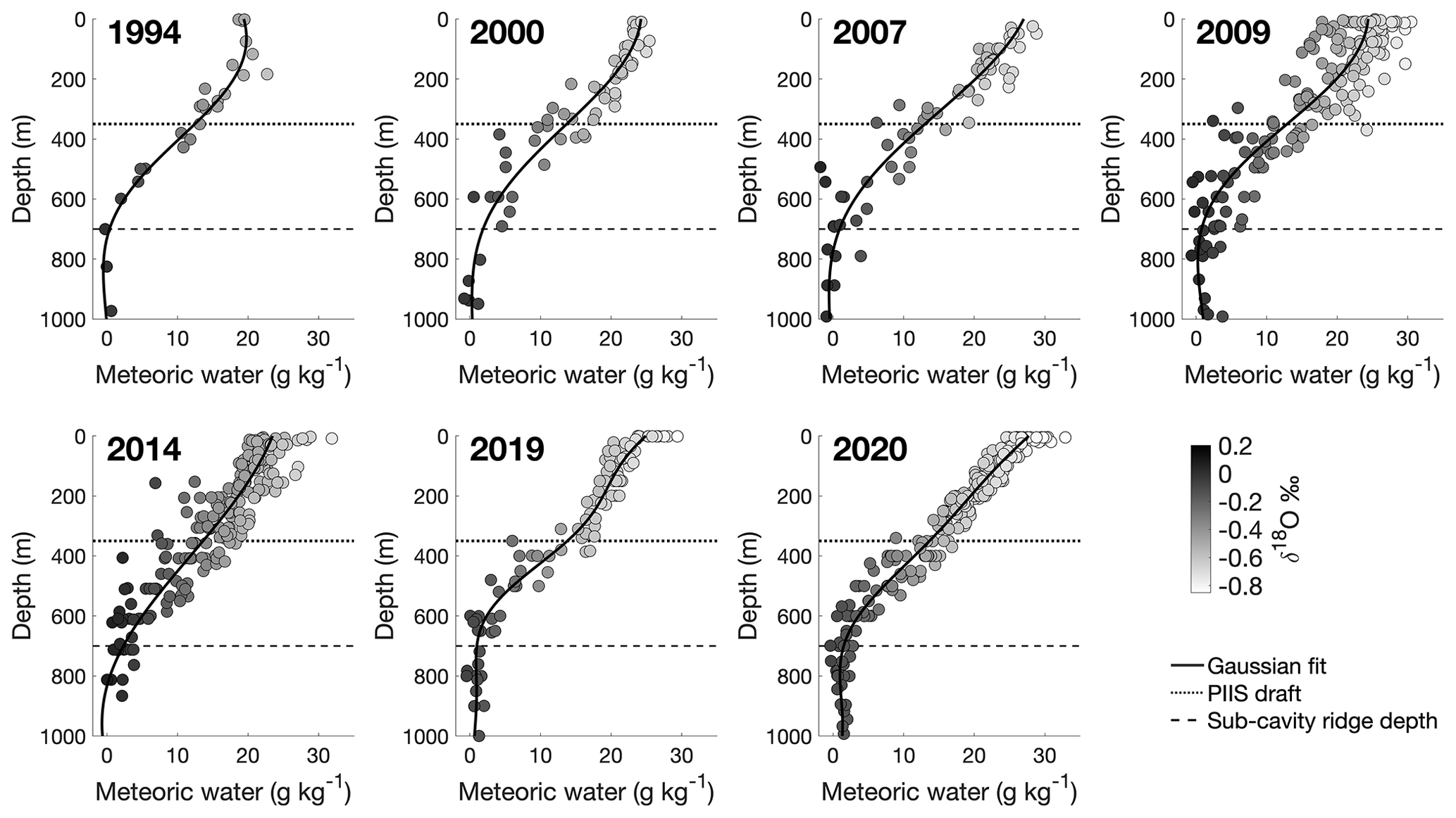
Figure 3 Meteoric water fractions (grams of meteoric water per kilogram of seawater) vs. depth. Shading shows the δ¹⁸O value and solid lines represent Gaussian process regression fits. Dotted and dashed horizontal lines show the depth of the PIIS draft and sub-cavity ridge, respectively (Jenkins et al., 2010). Small false-negative meteoric water fractions in deep waters are the result of sample salinity and/or δ¹⁸O values that are higher than the mCDW end-member value(s) (Table 2, Sect. 2.2) – the result of spatial variability in mCDW properties (discussed in further detail in Sect. 3.5).

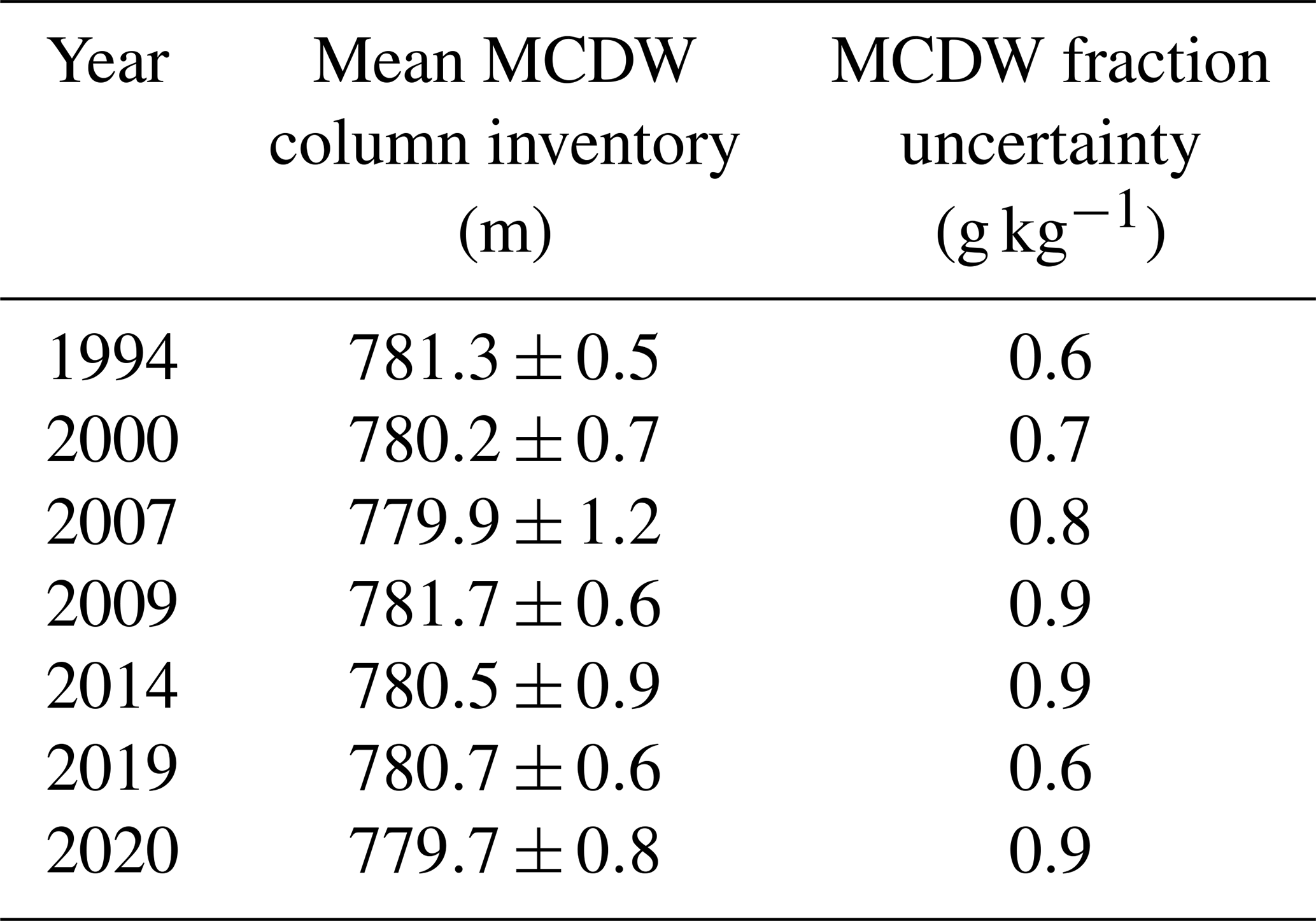
Evidence of highly δ¹⁸O-depleted freshwater is found at depths above ∼700 m (the depth of PIIS sub-ice-shelf ridge; Jenkins et al., 2010), with the highest concentrations found at depths shallower than 350 m – above which glacial meltwater has been observed to flow out from beneath the ice shelf (Biddle et al., 2017; Naveira Garabato et al., 2017). Made less dense by the addition of GMW, such outflows rise through denser waters above, along ice shelf calving fronts, and strongly influence surface waters in this region (Dierssen et al., 2002; Mankoff et al., 2012; Thurnherr et al., 2014; Fogwill et al., 2015). Mean integrated total meteoric water column inventories (Table 3) range from a low of 8.1±0.7 m in 1994 to a high of 9.6±0.8 m in 2000 and 2020, with meteoric water fraction uncertainty (described in Sect. 3.5.1) ranging from 1.4 g kg⁻¹ in 2019 to 2.8 g kg⁻¹ in 2009.

Table 3 Meteoric water column inventory and uncertainty. Depth-integrated meteoric water content using the Gaussian process fit (Fig. 3) between the sea surface and 800 m depth. Uncertainties are associated with instrumental precision, spatial variability in the data, and end-member uncertainty (Sects. 2.2 and 3.5).

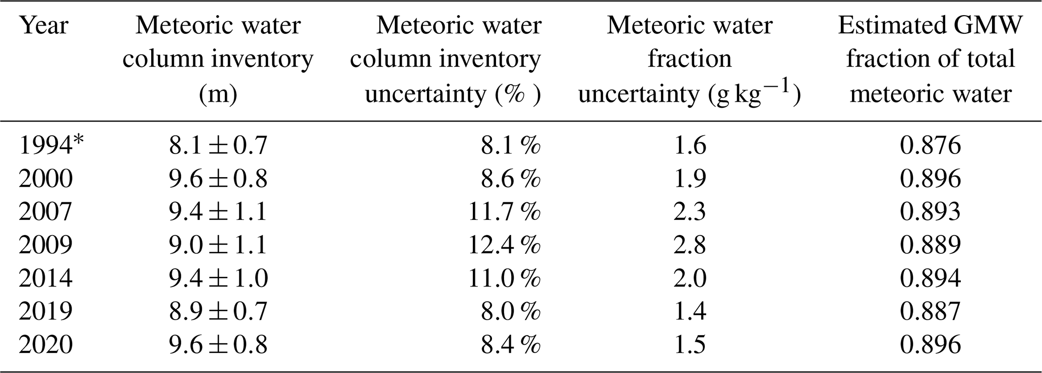
^* As 1994 has only four sampling locations and the strongest fit of any year (Fig. 2), its uncertainty may be artificially decreased.

3.3 Sea ice melt

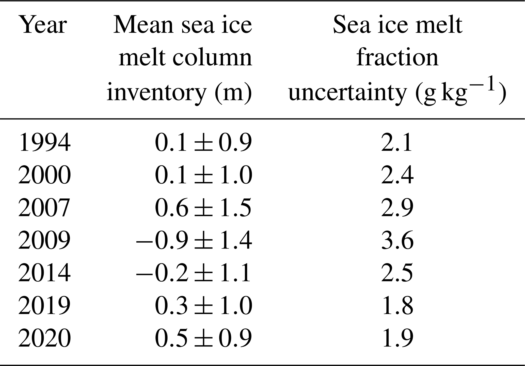
Sea ice melt fractions reach as high as 40 g kg⁻¹ in the upper surface waters (2019; Fig. 4), while sea ice melt fractions are mostly negative below 100 m, with the minima (i.e., largest negative fraction) occurring just above 200 m in most years. Negative sea ice melt fractions in subsurface waters are produced during sea ice formation (with the opposite signal produced in the near-surface when the sea ice melts) and reach as low as −13 g kg⁻¹. Larger positive sea ice melt fractions below 200 m correspond to samples with higher δ¹⁸O than others at a similar depth/salinity. Total integrated mean sea ice melt (Table 4) is near 0 across all years, with uncertainty (described in Sect. 3.5.1) in sea ice melt fractions ranging from 1.8 g kg⁻¹ in 2019 to 3.6 g kg⁻¹ in 2009. Mean sea ice melt inventories are influenced largely by very high fractions near the surface, potentially the result of sea ice melt “flooding” and import of sea ice melt from areas upstream (Ackley et al., 2020). Sea ice melt is discussed further in Appendix A5.

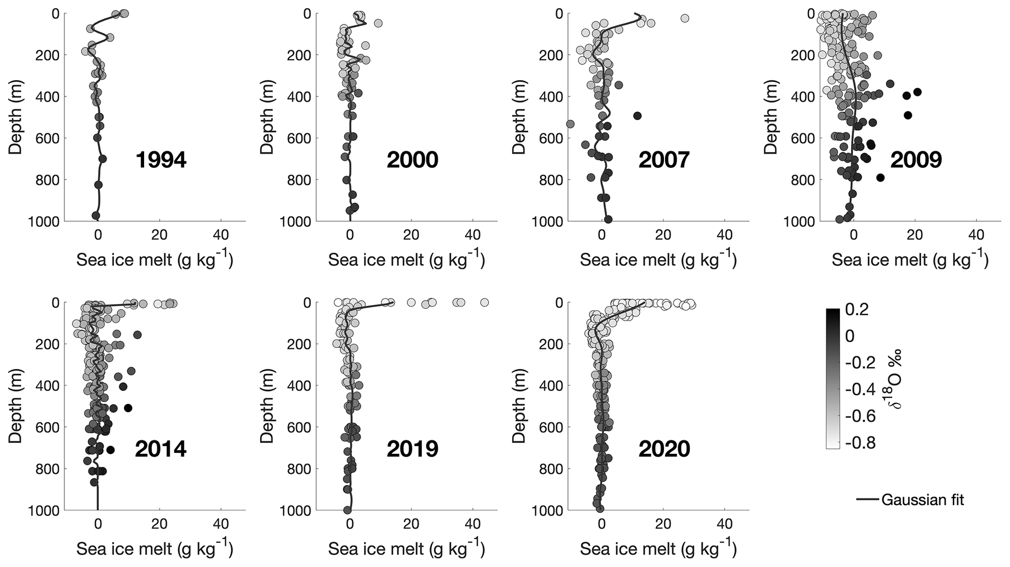
Figure 4 Sea ice melt fractions (grams of sea ice melt per kilogram of seawater) vs. depth. Shading shows the δ¹⁸O value and solid lines represent Gaussian process regression fits. Sea ice melt fractions are highest at the surface. Negative sea ice melt fractions, occurring mostly below 100 m, are the product of earlier sea ice formation.

Table 4 Sea ice meltwater column inventory and uncertainty. Depth-integrated sea ice meltwater content using the Gaussian process fit (Figs. 4, 3) between the sea surface and 800 m depth. Uncertainties are associated with instrumental precision, spatial variability in the data, and end-member uncertainty (Sects. 2.2 and 3.5).

3.4 Average meteoric water inventory over the last 2 decades

Average meteoric water column inventories (Table 3) in the study area were estimated by depth integrating the Gaussian process fit of the calculated meteoric water fractions (solid lines in Fig. 3). Figure 5 plots the mean meteoric water inventory in each year, with uncertainty described in Sect. 3.5. The average meteoric water column inventory was relatively low in 1994 and higher from 2000 to 2020. Strongly influenced by the low meteoric water inventory in 1994, a linear regression of the mean meteoric water inventories suggests an increase of 0.03±0.02 m yr⁻¹ (p value 0.25). The increase is small and, given the magnitude of the uncertainty associated with these inventories, may be (1) an artifact stemming from spatial sampling bias or (2) some fraction of a meteoric water signal imported from upstream.

These results show greater interannual variability than increasing trend in meteoric water content; however, they are consistent with recent modeling showing an increase in basal melt through the 1990s, followed by relative stability and interannual variability from 2000 through 2020 (Flexas et al., 2022). Meteoric water column inventories have uncertainties of <1.1 m (<12.4 %), accounting for analytical precision, end-member uncertainty, and spatial variability in the model inputs (Sect. 3.5). Based on very liberal evaluation of precipitation influence, these total meteoric water column inventories are likely to consist of >87 % GMW (Sect. 2.2, Appendix A4). While the glacial fraction of these results will include local and nonlocal iceberg melt, it will not include ice shelf losses via iceberg calving where icebergs melt outside of the study area.

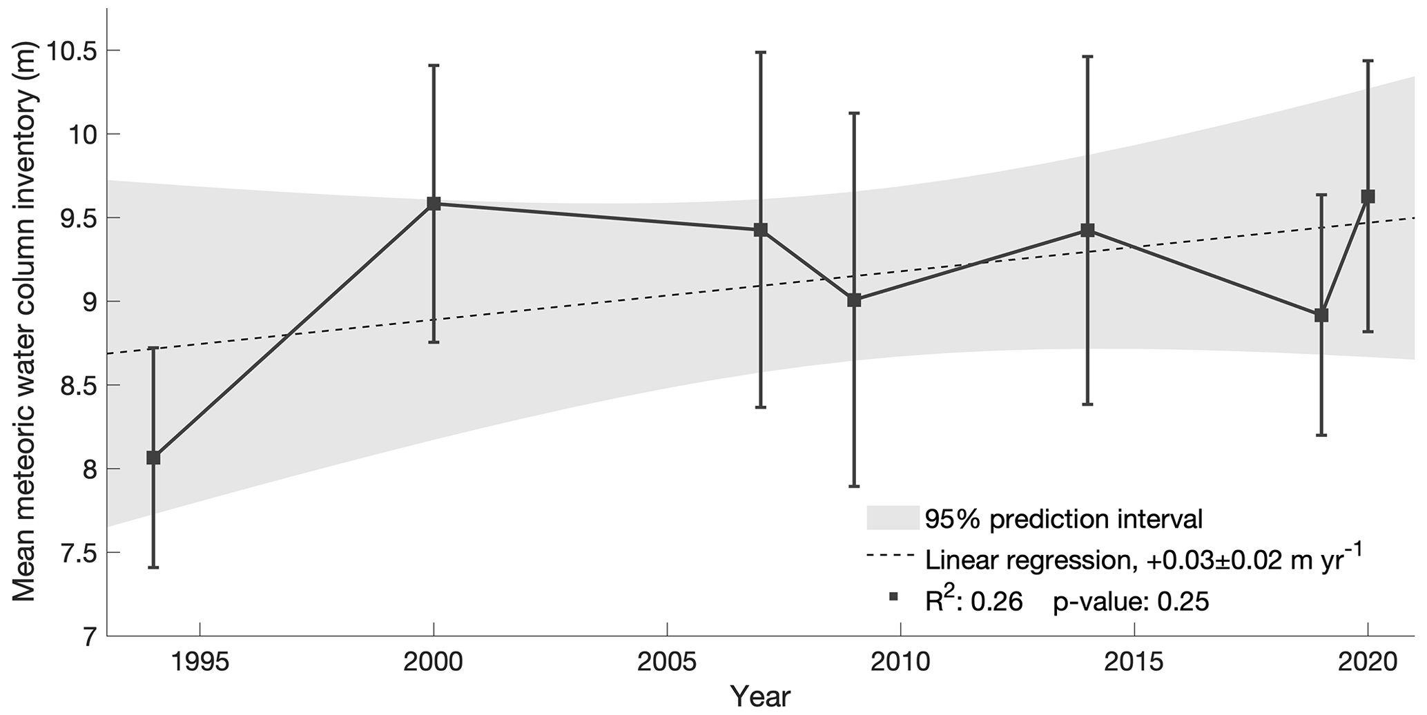
Figure 5 Average meteoric water column inventory. Depth-integrated meteoric water content from the Gaussian process fit (Fig. 3) between the sea surface and 800 m. Error bars show the uncertainty (Sect. 3.5) associated with data volume, analytical precision, and uncertainty in end-member values (Sect. 2.2). A linear regression of the mean values shows an increase of 0.03±0.02 m yr⁻¹ (p value 0.25). Gray shading shows the 95 % prediction interval for the linear regression.

3.5 Uncertainty and sensitivity analyses

3.5.1 Analytical precision, geographic sampling variability, and end-member uncertainty

The results of the three-end-member mixing model depend on the inputs and end-members used – all of which are subject to some level of uncertainty. We ran 15 000 Monte Carlo simulations for each year's data to assess the uncertainty of the results. In each simulation, we select three stations at random. Each observation is perturbed randomly by the precision associated with analytical precision for that instrument. We determine mCDW and meteoric water end-members from those perturbed data from the random selection of three stations; these two end-members will differ with each simulation, both due to the observational data perturbations and due to the randomized station selection. We apply an additional perturbation to all three end-members based on the uncertainty and variability associated with that end-member. In the upper 200 m of the water column, the precipitation fraction and the δ¹⁸O value are perturbed independently, in addition to the perturbations made to the meteoric GMW end-member calculated from the mixing lines (Fig. 2, Table 2). The greatest single source of water fraction uncertainty is end-member uncertainty, followed by geographic sampling variability. More in-depth details of the uncertainty analysis, perturbations used, and breakdowns of different uncertainty impacts can be found in Appendix A3.

Uncertainty in mean meteoric water fractions ranges from 1.4 g kg⁻¹ in 2019 to 2.8 g kg⁻¹ in 2009, and uncertainty in mean meteoric column inventories ranges from 7.9 %–12.4 %. Calculated water fractions are most strongly influenced by changes made to the mCDW end-member (comprising ∼99 % of an 800 m water column on average or ∼95 % in surface waters rich in meteoric water and sea ice melt). Sea ice melt and meteoric water fractions vary inversely. Meteoric water fractions also vary inversely with the magnitude of the meteoric water end-member δ¹⁸O (i.e., a more negative meteoric water end-member will produce smaller meteoric water fractions). The year 1994 has the fewest samples but the strongest fit (Fig. 2), so uncertainty for this year may be artificially low (Fig. 5).

3.5.2 Geographic variability by grouping

This study relied on the compilation of data collected for six independent studies over seven different cruises. To determine the impact of inconsistency in sampling locations each year, we conducted a spatial sensitivity analysis by separately analyzing different spatial groups of stations across each year (Fig. 6; Tables 5, 6), running 5000 Monte Carlo analyses for each group (as described in Sect. 3.5.1). Uncertainty is represented as the standard deviation of those results (Tables 5, 6).

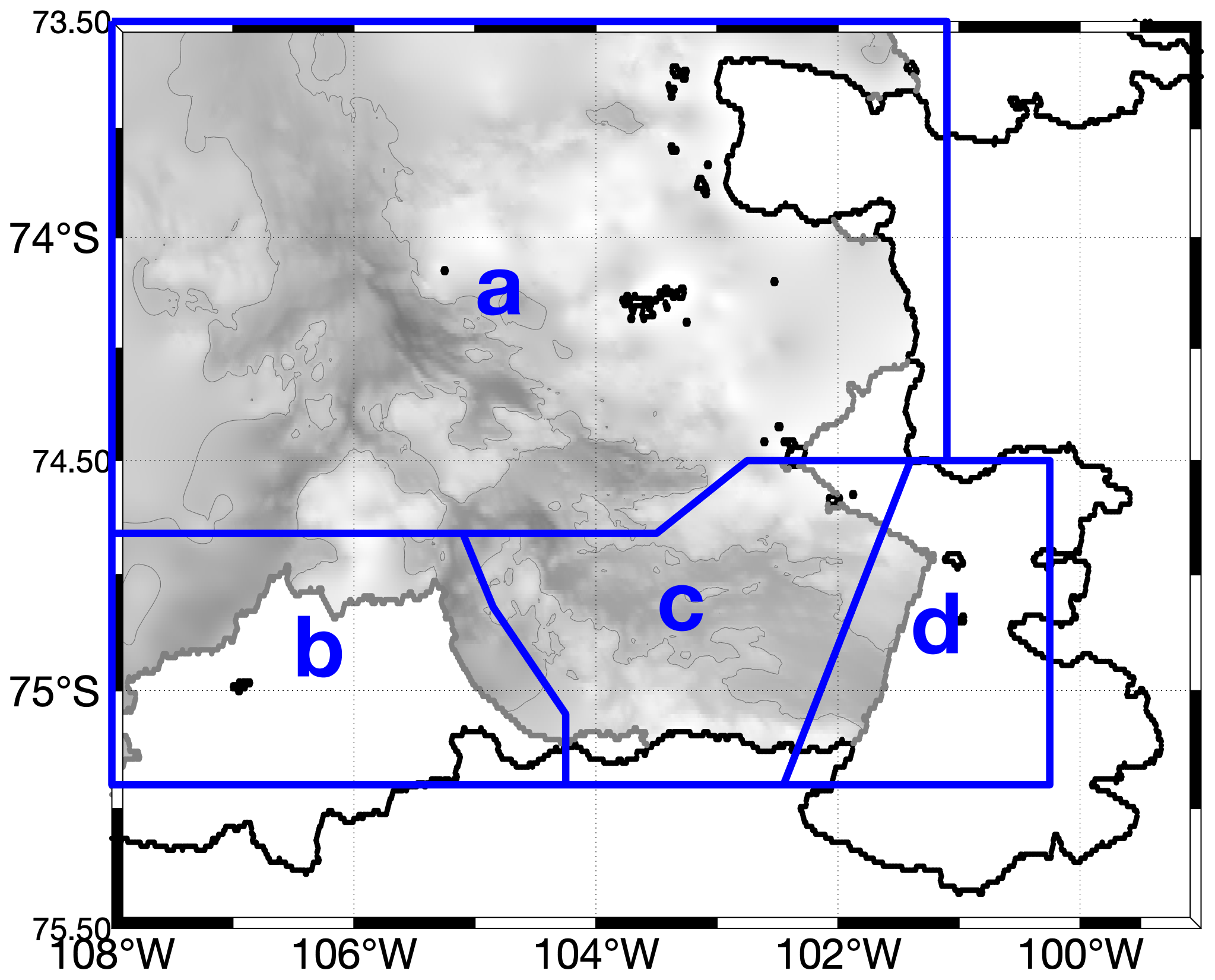
Figure 6 Boundaries of the geographic groupings used for spatial sensitivity analysis. Blue lines show the boundaries of geographic areas analyzed separately. Gray shading shows bathymetry, with isobaths drawn at 800 m. More detailed maps for each year are given in Appendix A4.1.

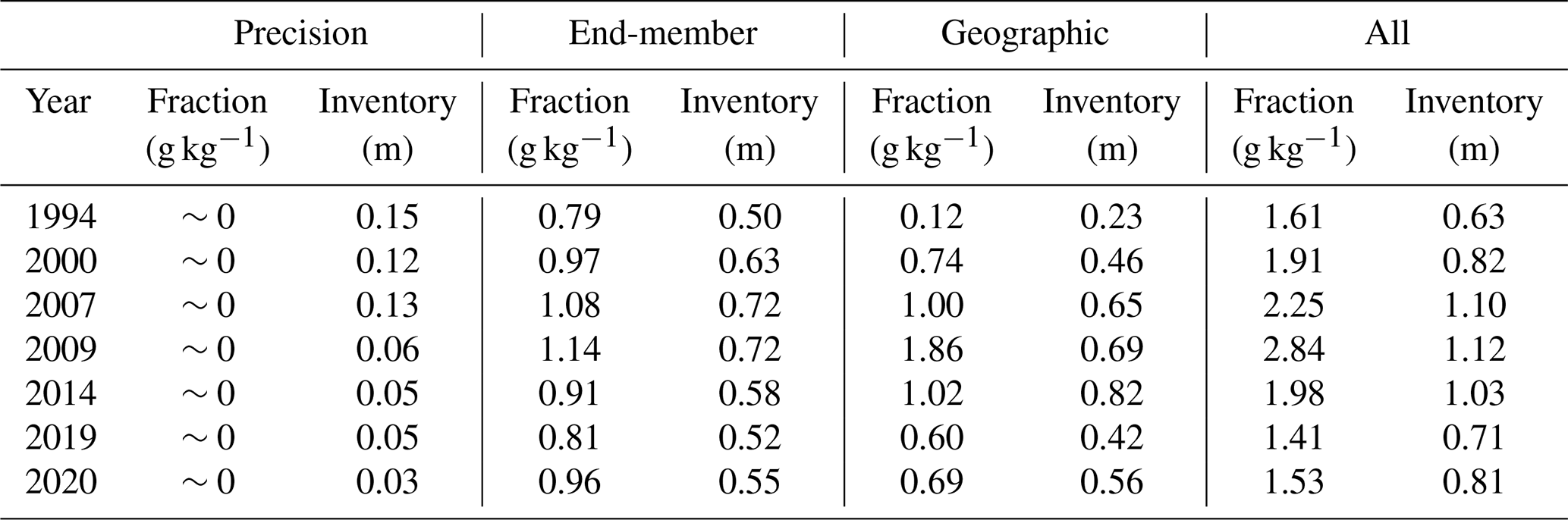
Table 5 Summarized results of the meteoric water column inventory (m) from spatial sensitivity analysis (Fig. 6). Results are given by year (in rows) and by area group (in columns). See Appendix A3.3 for further detail.

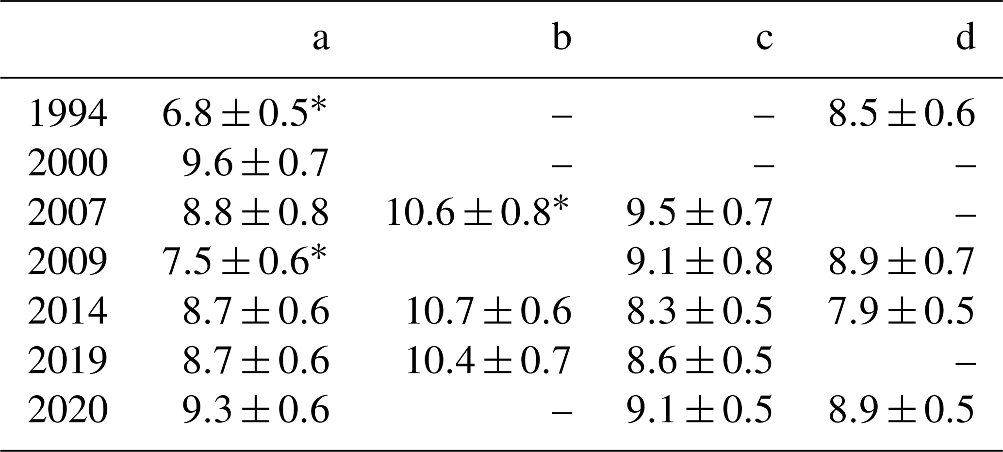
^* Data from only one station. For 1994, 2007, and 2009, the result is based on only eight, four, and four samples, respectively.

Table 6 Summarized results of the sea ice meltwater column inventory (m) from spatial sensitivity analysis (Fig. 6). Results are given by year (in rows) and by area group (in columns). See Appendix A3.3 for further detail.

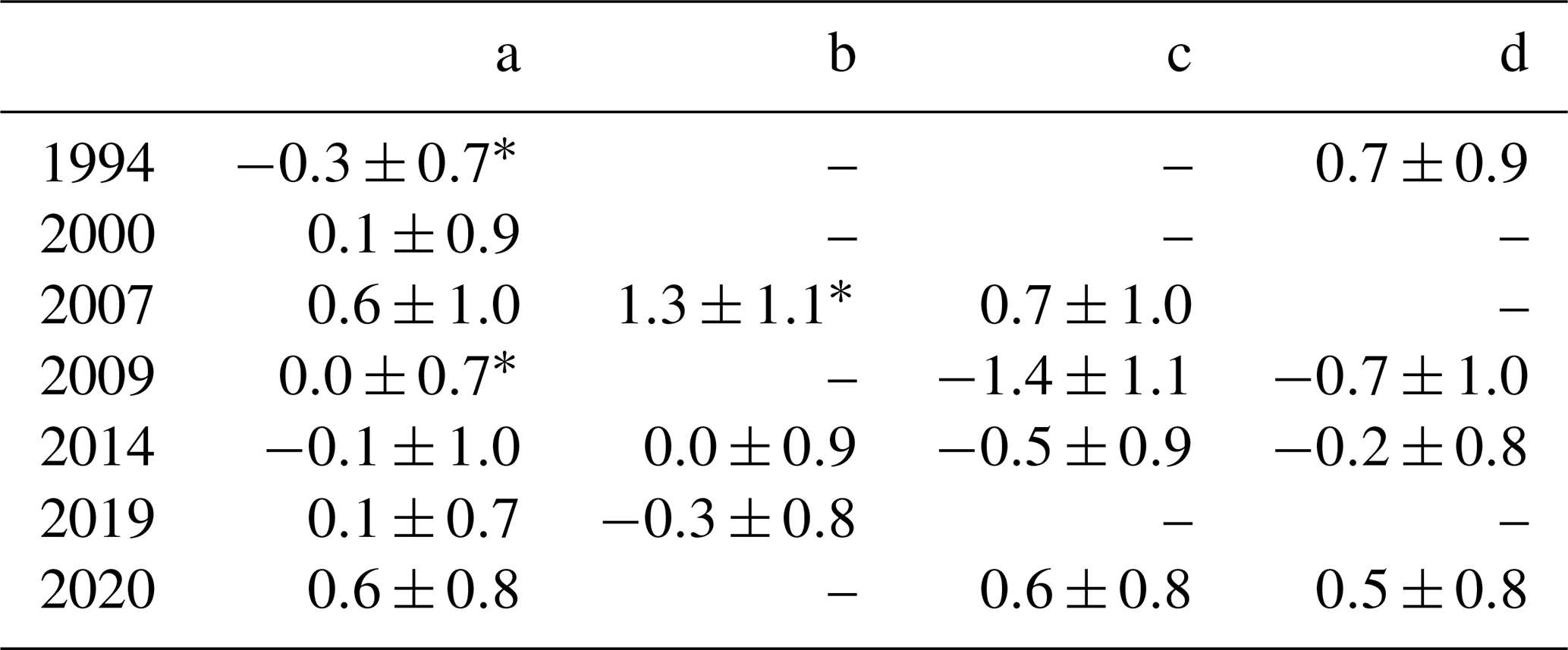
^* Data from only one station. For 1994, 2007, and 2009, the result is based on only eight, four, and four samples, respectively.

Grouped geographic sensitivity analyses show little spatial variability in mean water column inventories, accounting for uncertainty (Tables 5, 6). Mean sea ice melt inventories are consistently ∼0 m, with near-complete overlap of means and uncertainty envelopes across groupings for each year. Mean meteoric water column inventories are remarkably consistent spatially, except those calculated from stations in Group “a” in 1994 and 2009, where very few data were available, and Group “b” alongside Thwaites Ice Shelf (TIS), which showed significantly higher meteoric water inventories than the rest of the study area. Only one and two stations alongside TIS were sampled in 2007 and 2019, the average column inventories are consistent with the 2014 data, where there were eight stations in Group “b”. The higher inventories in Group “b” are suggestive of an accumulation of basal melt and are consistent with the findings from another study showing that basal melt from beneath PIIS ends up along the eastern edge of TIS (Wåhlin et al., 2021).

In some cases (e.g., 2020), the calculated mean meteoric water inventories from the individual groupings (Table 5) are higher than the overall mean. The apparently lower meteoric water column inventories result from small differences in calculated end-members (i.e., less-salty mCDW, more negative mCDW δ¹⁸O, and/or more negative meteoric water δ¹⁸O), as mCDW and meteoric end-members are defined separately for each geographic grouping in each year. The relative insensitivity of sampling location (with the exception of those alongside TIS) in calculated mean meteoric water column inventories suggests that precise reoccupation may be unnecessary and that a relatively small number of strategic stations/sampling locations could potentially be used to reliably assess mean meteoric water column inventory in this region; see Appendix A3.3 for detailed results, including individual end-members for each grouping.

4 Discussion

4.1 The utility of zero-salinity δ¹⁸O intercepts

The meteoric water end-member has been described as the least well-constrained component (Meredith et al., 2008, 2010, 2013; Randall-Goodwin et al., 2015; Biddle et al., 2019) of the three-end-member mixing model employed here, leading previous studies to use plausible mean meteoric δ¹⁸O values, falling between the δ¹⁸O value of glacial melt and local precipitation. We use linear regressions through salinity–δ¹⁸O mixing lines (e.g., Fig. 2) to determine glacial freshwater end-members (Fairbanks, 1982; Paren and Potter, 1984; Potter et al., 1984; Jacobs et al., 1985; Hellmer et al., 1998; Jenkins, 1999). The salinity–δ¹⁸O data presented here (Fig. 2) show clear mixing lines between mCDW and meteoric freshwater at depths below 200 m, with a δ¹⁸O value indicative of local glacial freshwater (Steig et al., 2005; Schneider et al., 2006). The uncertainty associated with these intercepts is lower than the mass-weighted standard deviation of the average δ¹⁸O of the ITASE 01-2 ice core (Fig. 2). Winter water, a salty, relatively δ¹⁸O-depleted product of sea ice formation, has a less δ¹⁸O-depleted signature than those influenced by GMW (Jenkins, 1999), and a liberal removal of samples that may be considered winter water ($\mathrm{\Theta }<\mathrm{1}.$5 ^∘C) has insignificant (<0.5 ‰) effect on the calculated intercepts.

The 2014 data presented here were previously used in another study (Biddle et al., 2019), where they selected −25 ‰ as a meteoric water δ¹⁸O end-member, adopting the midpoint between the GMW and precipitation δ¹⁸O values from another study further to the west (Randall-Goodwin et al., 2015). For the 2014 data, the current study uses base meteoric δ¹⁸O end-members of −31.3 ‰ for deep waters and of −27.3 ‰ for the upper 200 m (Table 2). Using a less negative end-member (as in Biddle et al., 2019) results in higher meteoric water fractions and lower sea ice melt (or increased sea ice formation) fractions, very likely overestimating the deep water column meteoric water content, which will consist of nearly pure GMW. We estimate that >73 % of the meteoric water in the upper 200 m is comprised of GMW (Sect. 4.2, Appendix A4). Determining the deep meteoric water (GMW) end-member using the better-constrained zero-salinity δ¹⁸O intercept of the sample data mixing line (Sect. 2.2) as well as a separate shallow meteoric end-member (incorporating a realistic precipitation fraction) provides more-accurate estimates of both meteoric water and sea ice melt fractions throughout the water column. The length of the intercept extrapolation emphasizes the importance of careful sample collection, storage and of high-precision analyses.

4.2 Glacial meltwater and precipitation

The δ¹⁸O values of local precipitation and glacial melt are significantly different from one another and can be clearly distinguished on the basis of δ¹⁸O. On George VI Glacier, Potter and Paren (1985) observed that the ice flux into the ice shelf had a δ¹⁸O value of $\sim -\mathrm{20}\mathrm{‰}$, whereas accumulation of precipitation onto the northern form of the ice shelf was much less depleted, with a δ¹⁸O of $\sim -\mathrm{13}\mathrm{‰}$. Precipitation grows increasingly depleted in ¹⁸O with latitude (Dansgaard, 1964; Gat and Gonfiantini, 1981; Ingraham, 1998; Masson-Delmotte et al., 2008) and altitude (Dansgaard, 1964; Friedman and Smith, 1970; Siegenthaler and Oeschger, 1980; Ingraham, 1998; Araguás-Araguás et al., 2000; Sato and Nakamura, 2005; Masson-Delmotte et al., 2008). A total of 88 % of the spatial variation in the δ¹⁸O of Antarctic precipitation can be explained by linear relationships between latitude, elevation, and distance from the coast, with elevation being the primary driver (Masson-Delmotte et al., 2008). Precipitation collected during the NBP19-01 cruise in the study had a δ¹⁸O value of −15 ‰, consistent with other data from that latitude and elevation. Precipitation is discussed further in Appendix A4.

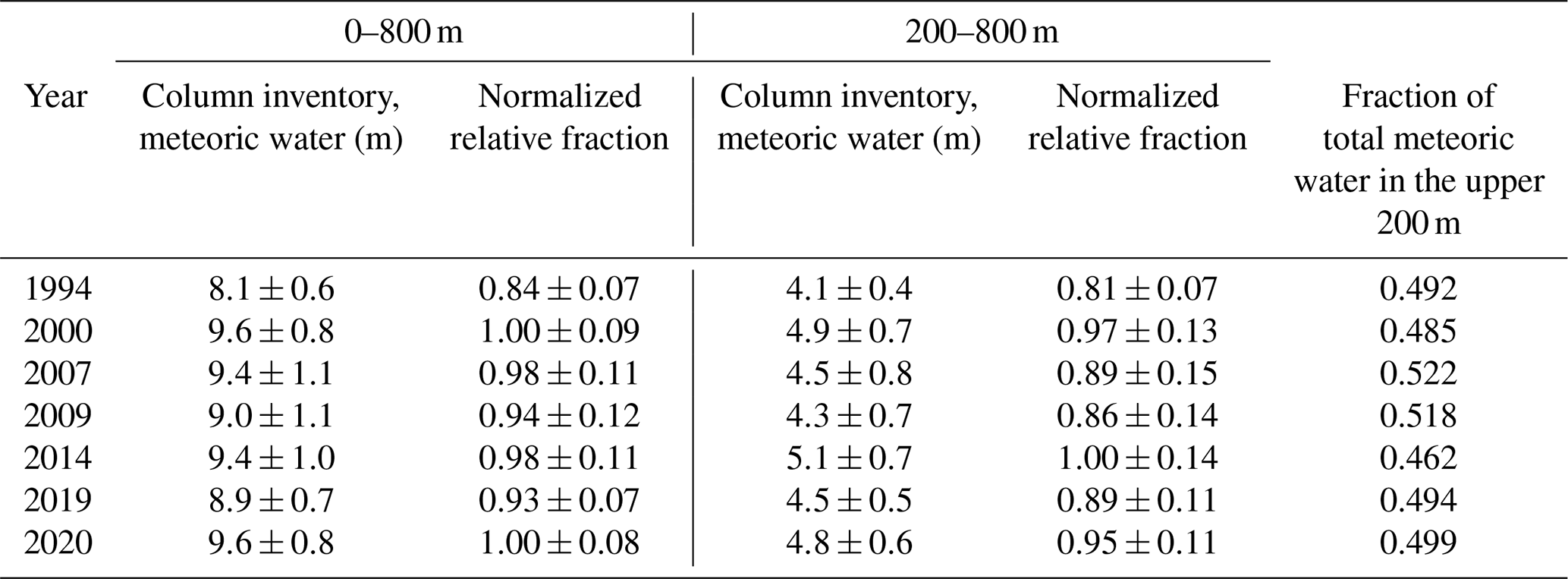
The nearest ice cores to our site, ITASE 01-2 (Steig et al., 2005; Schneider et al., 2006) and Siple (Mosley-Thompson et al., 1990), have average δ¹⁸O compositions of $-\mathrm{29.8}\pm \mathrm{1.9}\mathrm{‰}$ (ITASE 01-2) and $-\mathrm{29.6}\pm \mathrm{1.1}\mathrm{‰}$ (Siple). Using locally collected salinity and δ¹⁸O data from deeper than 200 m to calculate a zero-salinity intercept, we identify average freshwater end-members ranging from $-\mathrm{31.3}\pm \mathrm{1.0}\mathrm{‰}$ to $-\mathrm{28.4}\pm \mathrm{1.0}\mathrm{‰}$ (mean 29.4±1.0 ‰). The similar zero-salinity intercept and the strong linear salinity–δ¹⁸O relationship below 200 m demonstrate that glacial freshwater is responsible for the observed freshening signal. We find roughly half of the total meteoric water inventory in the upper 200 m, below which inventories yield the same relative trend in interannual variability (Appendix A5), indicating that the observed variability results from changes in glacial meltwater content, not from interannual variability in local precipitation. A substantial fraction of precipitation (both local and nonlocal) will be deposited on sea ice, much of which is subsequently advected out of the study area, (Assmann et al., 2005), and, as a result, has no impact on locally measured meteoric water content, suggesting that GMW could comprise an even greater fraction than the base level used here (Table 2).

Nearly half of the water column meteoric water content resides in the upper 200 m, and >73 % of that meteoric water is comprised of glacial meltwater (Appendix A5). The use of a midpoint GMW–precipitation intercept will overestimate GMW fractions through the water column, directly impacting the accuracy of other techniques using δ¹⁸O GMW measurements for calibration (Pan et al., 2023). While previous studies (Randall-Goodwin et al., 2015; Biddle et al., 2019) have not quantified GMW in the upper 100–150 m of the water column due to uncertainty surrounding the impact of local precipitation, our analysis indicates that precipitation comprises a relatively small fraction of even upper water column meteoric water, even in the most extreme case. The two-component meteoric end-member approach presented here accounts for a fraction of precipitation in the upper water column, providing more-accurate meteoric water and sea ice melt fractions for both deep and shallow waters as well as more-accurate estimates of full column meteoric water (and GMW) inventories.

4.3 Temporal changes in mean meteoric water column inventories

We estimated average meteoric water column inventories in the SE Amundsen Sea seawater oxygen isotopes and salinity using a two-component meteoric water end-member approach in the three-end-member mixing model (Sect. 2.2). In 1994, 2007, 2014, and 2020, there is a tendency for the maximum integrated meteoric water volume to extend westward from the southwestern corner of the PIIS and along the eastern TIS (Fig. 1), consistent with the gyre-like circulation there (Thurnherr et al., 2014). This pattern of meteoric water distribution is consistent with local GMW patterns previously observed using traditional hydrographic tracers (Thurnherr et al., 2014; Naveira Garabato et al., 2017; Wåhlin et al., 2021).

Local meteoric water content varies from a low of 8.1±0.7 m in 1994 to high values of 9.6±0.8 m in 2000 and 2020. Inventories fluctuated over the latter period, without apparent trend, depending on the spatial and temporal coverage of available datasets. The inventories presented here are likely to include some fraction of meteoric water (in the form of precipitation and GMW) imported from upstream; however, the consistency of our zero-salinity δ¹⁸O intercepts with local ice core values suggests that the meteoric water estimated in this study is predominantly local in source. While salinity and δ¹⁸O alone cannot be used to determine basal melt rates, the average meteoric water inventories are sufficient to identify relatively small changes in melt rates, assuming a constant residence time.

The mCDW entering the SE Amundsen Sea and accessing the underside of the ice shelves has been shown to exhibit little seasonal variability, with a maximum variance in T of <0.1 ^∘C, S of <0.05 g kg⁻¹, and thickness of <50 m (Mallett et al., 2018). All samples used in this study were collected from 12 January to 15 March, when melt rates for the PIIS and TIS exhibit very little seasonal variability (Kimura et al., 2017). With a residence time of ∼2 years (Tamsitt et al., 2021), it is unlikely that the variability in yearly meteoric water column inventories is a product of a seasonal signal.

While the meteoric water inventories presented here are not equivalent to melt rates, they should be indicative of relative year-to-year changes in melt rates. Our mean meteoric water inventories suggest an increase in melt rates after 1994 followed by relative stability, with greater year-to-year variability than the trend in melt rates across the years covered by the study data. We find the lowest mean meteoric water inventory in 1994, whereas other studies using hydrographic data estimate 1994 as an average melt year for PIG – lower than 2007 and 2009 but higher than 2014 (Joughin et al., 2021b). Another study identified a slowdown in melt rates between 1992 and 2017 (Paolo et al., 2023). One modeling study found a low basal melt flux in 1994 followed by a higher but variable flux through 2013 (where their simulation ends) under ERA5 forcing, while PACE forcing resulted in interannual variability over our study period but a high melt year occurring in 1994 (Naughten et al., 2022). Adusumilli et al. (2020) found an increase in basal melting between 1994 and 2000 followed by a peak in basal melt in 2009; however, their results show relative stability with significant interannual variability between 1994 and 2018. The pattern in mean meteoric water inventories presented in this study is most consistent with recent modeling efforts finding an increase in melting from 1993 to 2000, followed by relative stability in melt rates through 2019 (Flexas et al., 2022).

Glacial meltwater measured in the SE Amundsen Sea includes mCDW-driven basal melt, iceberg melt (some of which may consist of icebergs imported from upstream), and meltwater entering the ocean at the grounding zone that is driven by the geothermal heat flux to the base of the ice sheet (∼5.3 Gt yr⁻¹; Joughin et al., 2009). Other studies have noted an increase in ice sheet losses to iceberg calving in recent years (Joughin et al., 2021a), comprising a nontrivial component of ice sheet mass loss (Rignot et al., 2013; Greene et al., 2022) – any icebergs that are exported and melt outside of the study area (Mazur et al., 2019, 2021) will not contribute to the mean meteoric water inventories presented here. The greatest limitation of using average meteoric water inventories as a means for GMW accounting arises from the poorly constrained residence time of regional shelf waters, as there has been little study of this component. This uncertainty is further confounded due to the intensification of coastal circulation in the Amundsen Sea resulting from increased melt rates (Jourdain et al., 2017). With local circulation generally moving waters westward (Nakayama et al., 2013; Thurnherr et al., 2014; Naveira Garabato et al., 2017; Nakayama et al., 2019; Wåhlin et al., 2021; Dotto et al., 2022), it is likely that the calculated meteoric water fractions in the study area (with the exception of those on the western side of TIS) are primarily comprised of basal melt from PIIS.

While circulation and residence time are unknown and increasing melt rates may make them a moving target, the broad assumption that a mean residence time of 2 years (Tamsitt et al., 2021) and GMW comprising >87 % of total meteoric water column content (Appendix A4) are representative of the whole study area (∼30 000 km² ocean) produces GMW input estimates of between 106±17 Gt yr⁻¹ (1994) and 129±17 Gt yr⁻¹ (2000 and 2020). Although empirical, these figures are consistent with satellite-based estimates of mass loss from PIIS via basal melt (Rignot et al., 2013, 2019), demonstrating the potential utility of geochemical ocean measurements for estimating ice shelf melt rates and helping to calibrate and constrain larger-scale remote-sensing estimates.

5 Conclusions

We use seawater δ¹⁸O and salinity data collected in the SE Amundsen Sea from 1994 to 2020 to calculate inventories of meteoric (fresh) water through the water column. Freshwater intercepts from salinity–δ¹⁸O plots produce a well-constrained meteoric water end-member, consistent with measurements from regional ice cores and indicative of glacial meltwater. Using a meteoric water end-member determined by a regression through salinity–δ¹⁸O eliminates much of the uncertainty around meteoric end-members at depth. In the upper water column, using a meteoric water end-member comprised of glacial meltwater and a volume of local precipitation determined from local climatology, at an appropriate δ¹⁸O, produces more-accurate meteoric (and sea ice melt) water fractions both at depth and in the near surface than approaches taken by earlier studies. With cutting-edge advanced optical techniques using δ¹⁸O-based meteoric water measurements to calibrate their surface GMW estimates from satellite data (Pan et al., 2023), it is more important than ever that meteoric water fractions (entirely dependent upon selected end-members) estimated with δ¹⁸O are as accurate as possible. The application of local precipitation quantities and δ¹⁸O values to the meteoric water column inventories presented here has also allowed us to demonstrate that meteoric waters from the ocean surface to the floor are comprised primarily of glacial meltwater: >73 % in the upper water column and nearly 100 % in deep waters. While we have been very liberal with the inclusion of a high precipitation fraction in our analysis, a large portion of local precipitation is likely exported by sea ice without ever entering the surface ocean.

The WAIS is an important region for understanding sea level rise, as changes in winds and ocean circulation can increase basal melting of ice shelves as well as the flow of their ice streams into the sea. We present an advancement in end-member determination and application for use in the three-end-member mixing model over previous studies, producing more robust, well-constrained results, and suggest broader applications for these types of data. Changes in meteoric water inventories in the SE Amundsen Sea study region are consistent with satellite-based estimates of annual mass loss from the PIIS. These results demonstrate the potential utility of seawater δ¹⁸O and salinity data as an independent method for estimating ice shelf basal melt rates. While subject to an increased level of uncertainty due to the enhanced circulation resulting from increased ice shelf melt and potential influx of meltwater from upstream, monitoring meteoric water fractions and the use of average inventories can provide insight into the fast-changing conditions in the SE Amundsen Sea. Regular sampling for δ¹⁸O and salinity in this region could reveal if the existing record and its variability will extend into an era when ice shelves are likely to be thinner, with their grounding lines deeper and farther south. Integration of δ¹⁸O data into numerical models – with δ¹⁸O and associated meteoric water inventories used to constrain and calibrate ocean and ice sheet models and with model outputs informing ongoing δ¹⁸O sampling strategy – could further our understanding of ocean circulation and ice loss along this climatically sensitive sector of the WAIS.

Appendix A

A1 Defining mCDW

Modified Circumpolar Deep Water (mCDW) is one of three end-member waters that we use in a mixing model to determine glacial meltwater fractions, as the salinity and δ¹⁸O of mCDW are observationally well constrained, with interannual variability and properties that are defined separately for each year (as in Fig. A1 for 2020 data). Being the warmest, saltiest water on the continental shelf, mCDW appears at the top right-hand side on a T–S diagram (Fig. A1a), where it also identifies waters that are the least depleted with respect to δ¹⁸O.

In Fig. A1b and c, the same 2020 data show the keystone positions of mCDW in temperature–salinity–δ¹⁸O–depth space. The red and blue dashed lines show property mixing lines between mCDW, glacial meltwater (GMW), and sea ice melt, with the colder waters being fresher and more depleted in δ¹⁸O. Most data are above ∼800 m, with the least δ¹⁸O depletion in a few deep depressions. Waters that fall off the mCDW–GMW mixing line in the upper 200 m have been influenced by sea ice melt and atmospheric processes. Sea ice melt has a slightly positive (+2.1 ‰) δ¹⁸O, whereas GMW has a very negative ($\sim -\mathrm{30}\mathrm{‰}$) δ¹⁸O. Both freshen seawater, with the sea ice melt slightly counterbalancing the strong negative δ¹⁸O of GMW.

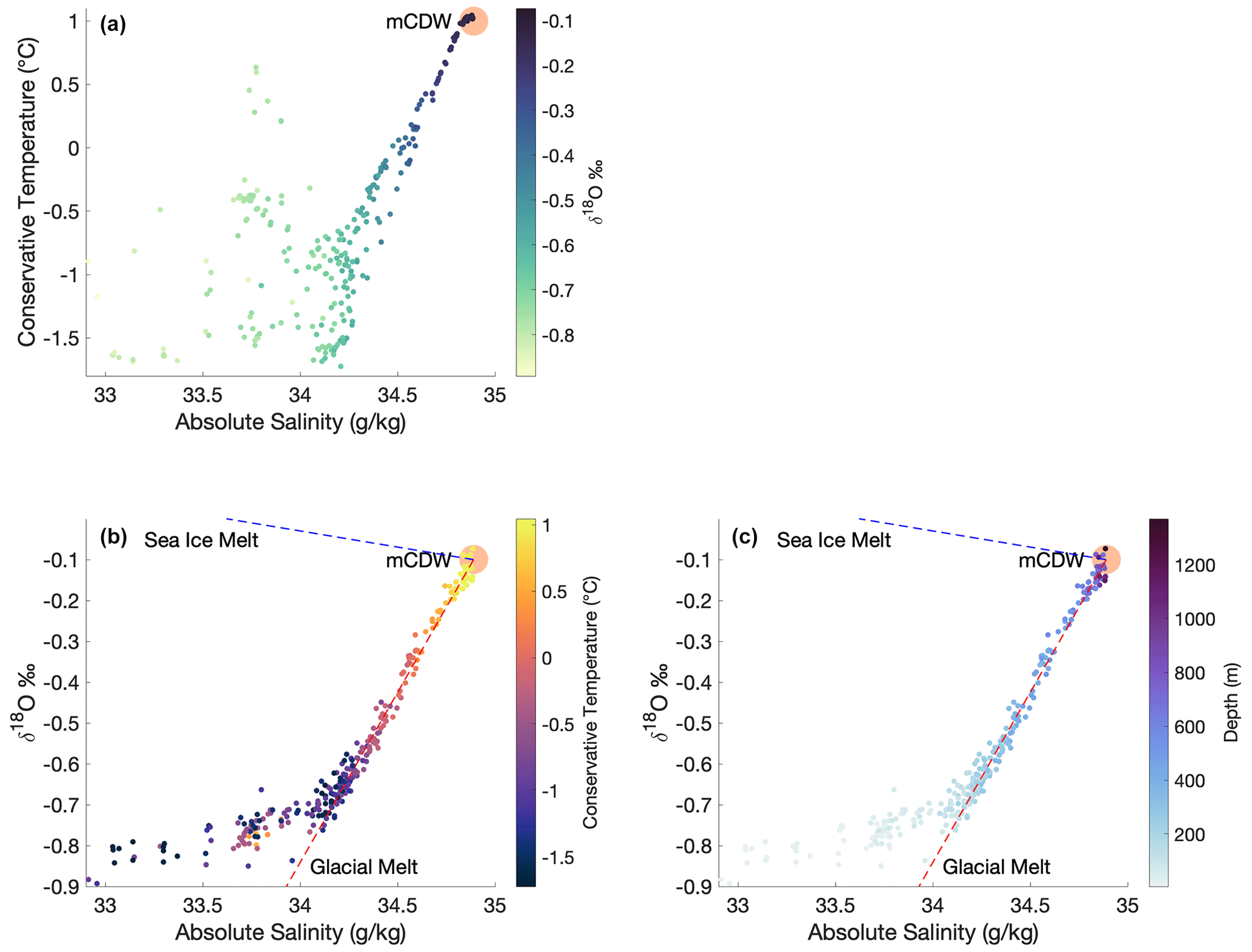
Figure A1 Temperature, salinity, δ¹⁸O, and depth from 2020 data. (a) T–S diagram with the color bar showing δ¹⁸O. (b) δ¹⁸O vs. salinity with the color bar showing temperature. (c) δ¹⁸O vs. salinity with the color bar showing sample depth. Data diverge from the mCDW–glacial melt mixing line at depths shallower than 200 m due to the presence of sea ice melt in the admixture. In panels (b) and (c), the dashed lines show the associated property mixing lines for mCDW mixing with sea ice melt or with GMW.

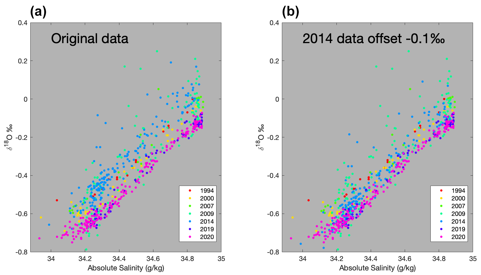
Figure A2 δ¹⁸O vs. absolute salinity for all years, from data >200 m. (a) All δ¹⁸O vs. salinity data, with the 2014 data as published in Biddle et al. (2019). Panel (b) is the same as panel (a) but with a −0.1 ‰ offset correction applied to the 2014 data.

In Fig. 2 of the main text, δ¹⁸O–salinity plots for each year reveal several data points near the salinity maximum, with some variability in the corresponding δ¹⁸O. Below 200 m, trend lines extrapolated to zero-salinity intercepts define the mCDW and meteoric water (GMW) end-members used in the mixing model. mCDW and meteoric water δ¹⁸O are defined at the salinity maximum and zero-salinity intercepts of the trend lines (Table 2). The mCDW location corresponds to conventional measures of the deepest and warmest waters on the continental shelf. The calculated zero-salinity intercept values are consistent with the properties of locally available GMW.

A2 Interlaboratory offsets

δ¹⁸O data from different laboratories are subject to possible systematic offsets. For example, a ∼0.1 ‰ δ¹⁸O offset between the 2014 data and other years (Fig. A2) is likely the result of an interlaboratory calibration offset. On the other hand, greater scatter in the 2009 data suggests that evaporation during sample storage left some samples less depleted with respect to δ¹⁸O. Here, we primarily compare calculated meteoric water fractions rather than δ¹⁸O values, with mCDW and meteoric water signatures defined separately for each year so that any offset will not affect the values of samples from that year relative to their mCDW and meteoric water signatures.

Using a sensitivity analysis, all sample data from a given year were offset and mCDW/meteoric water signatures were recalculated using the offset data. The result and end-members were used to calculate meteoric water fractions in the three-end-member mixing model, with sea ice melt values remaining static. We found that an offset of 5.7 ‰ δ¹⁸O (Fig. A3) would be necessary to change the calculated meteoric water fraction by an amount greater than the analytical precision (±0.04 ‰ δ¹⁸O, ±0.003 g kg⁻¹ for salinity) and environmental uncertainty based on ice core measurements (±1.9 ‰ for δ¹⁸O) and year-to-year variability in mCDW values (±0.06 ‰ δ¹⁸O). Interlaboratory offsets should be less than 0.1 ‰ (Walker et al., 2016), so any offsets will not be significant when comparing calculated meteoric water fractions.

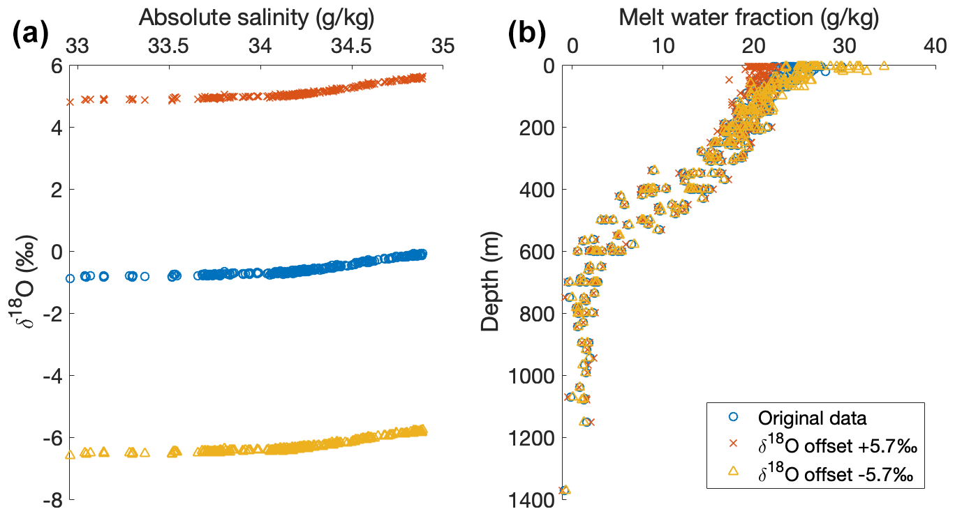
Figure A3 Impact of interlaboratory offsets on the calculated meteoric (glacial melt) water fraction for NBP20-02 data. Panel (a) shows the δ¹⁸O offset (±5.7 ‰) necessary to significantly affect the calculated meteoric water fractions, when using mCDW and meteoric water end-members calculated from those data. Panel (b) shows the calculated meteoric water fractions produced using the original and the offset data. The calculated meteoric water fractions are impacted very little because two of the three end-members (mCDW and meteoric water) are defined by the offset data.

A3 Uncertainty and sensitivity analyses

As meltwater fractions are calculated using analytical measures of salinity and δ¹⁸O, the accuracy and precision of these measurements are important. CTD salinity sensors have a reported precision of ±0.002. The isotope ratio mass spectrometer (IRMS; 1994 to 2014) measurements have a measured precision of ±0.04 ‰ based on replicates, whereas the CRDS system achieved a precision of ±0.02 ‰. The meteoric (GMW) end-member is arguably the least well constrained, with glacial ice in West Antarctica ranging from −20 ‰ to −40 ‰, but much of that uncertainty has been eliminated by using the zero-salinity intercept determination on a δ¹⁸O–salinity mixing line, corroborated by nearby ice core values (as discussed in the main text). mCDW is well constrained, based on many accurate in situ measurements. Our sea ice melt end-member is adopted from previously published studies in the region (Meredith et al., 2008, 2010, 2013; Randall-Goodwin et al., 2015; Biddle et al., 2019).

A3.1 Precision and geographic sampling variability impact on end-members

mCDW and meteoric water end-members are determined from sample data. We tested the sensitivity of these end-member values to instrumental precision and geographic sampling variability. We ran a Monte Carlo analysis calculating results from random sets of three stations 15 000 times. For each group of three stations, mCDW and meteoric water end-members and average meteoric water column inventories were calculated using only those data. Stations with fewer than two samples >200 m were excluded. As the three-end-member mixing model is most sensitive to the mCDW end-member, a set of stations lacking samples >800 m (deeper than the sub-cavity ridge; “pure” mCDW) had a random mCDW sample from >800 m that year added to the dataset for analysis.

Table A1 Sensitivity of the mCDW and meteoric water end-members to instrumental precision and geographic sampling variability. mCDW is defined as the δ¹⁸O value at the salinity maximum on the linear regression of all salinity–δ¹⁸O measurements deeper than 200 m for each group of stations; meteoric water δ¹⁸O is defined as the zero-salinity intercept on that same line. Average meteoric water inventory is the depth integration of the Gaussian fit of all calculated meteoric water fractions within each group. In all cases, uncertainty is represented by the standard deviation in the results obtained across 15 000 Monte Carlo simulations for each year.

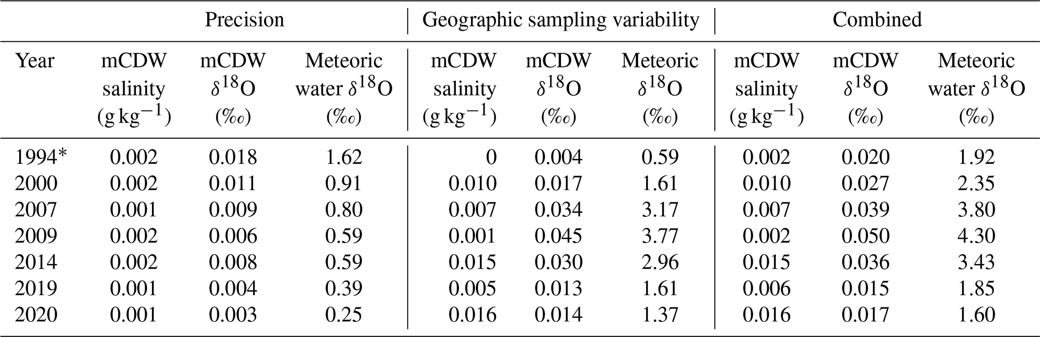
^* As 1994 has only four sampling locations and the strongest fit of any year (Fig. 2), its uncertainty may be artificially decreased.

mCDW properties display low geographic sensitivity, although 2009 and 2014 exhibit higher variability than other years, potentially due to sample collection and/or storage issues (Appendix A2, A6). Meteoric water end-member properties showed greater spatial uncertainty in 2007, 2009, and 2014. In these 3 years, the data show the greatest scatter, and mCDW samples were not always collected from the deep water column. The lengthy meteoric water end-member extrapolation benefits from many samples collected below 200 m, all the way to the seafloor. For 2014, spatial uncertainty is somewhat inflated due to the very high (>10 m) meteoric water inventories at stations immediately alongside TIS, while the 2009 data are impacted by sample storage issues and by poor depth resolution at some locations. In all cases, instrumental precision had an insignificant impact on end-member determination.

A3.2 Uncertainty in calculated meteoric water fractions

We use Monte Carlo simulations to estimate uncertainty in water mass fraction calculations. We ran 15 000 simulations, selecting 3 stations at random with input values varied randomly within these bounds, and represent uncertainty by the standard deviation of the difference between the simulated and initial runs. Observations were varied randomly by analytical precision for each run. mCDW and meteoric water end-members vary through each run, depending on the subset of stations selected (Table A1) and the perturbations made to the observational data. Additional perturbations are made to the end-member values, including sea ice melt (Table A2).

mCDW salinity varied by the results of a spatial sensitivity analysis (Appendix A3), and δ¹⁸O was varied by the 68 % prediction interval (1σ) of the >200 m δ¹⁸O–salinity relationship at the salinity maximum.

The GMW meteoric water end-member used for samples >200 m is additionally perturbed by the standard deviation of the ITASE 01-2 ice core – also consistent with the largest zero-salinity δ¹⁸O intercept standard error any year (2009). For those samples shallower than 200 m, the precipitation δ¹⁸O was perturbed by values with a standard deviation of 4.5 ‰ – the mean standard deviation of precipitation collected at sites in West Antarctica (IAEA/WMO, 2024) – and the GMW fraction was perturbed by 0.05.

The sea ice melt end-member is perturbed based on theoretical and experimental values (Rohling, 2013).

Perturbations used in the uncertainty analysis are summarized in Table A2, and the impacts on meteoric water fractions and column inventories are summarized in Table A3.

Table A2 End-member perturbations for uncertainty analysis. Perturbations are based on analytical precision for observations, the ITASE 01-2 ice core for meteoric water, and theoretical values for sea ice melt (Rohling, 2013). mCDW perturbations are based on the 68 % prediction interval (∼1σ) of the >200 m δ¹⁸O–salinity relationship at the salinity maximum, and salinity perturbations are based on the results of the spatial randomization analysis (Appendix A3). n/a – not applicable.

^a For 1994, we perturbed salinity by the average salinity standard deviation for the other years, to compensate for the smaller number of samples. ^b Mean effective perturbation across all years.

Table A3 Uncertainty in meteoric water fractions and column inventories resulting from different types of perturbations. Mean uncertainty in meteoric water fractions and column inventory associated with perturbations to each of the evaluated sources of uncertainty.

The mean uncertainty in meteoric water fractions ranges from ±1.4 g kg⁻¹ in 2019 to 2.8 g kg⁻¹ in 2009, corresponding to average meteoric water column inventories uncertainty between ±0.5 m in 2019 and ±0.7 m in 2009 (Table A3). Meteoric water and sea ice melt fractions vary inversely, whereas mCDW fractions remain relatively stable. Calculations are most impacted by changes to the mCDW endpoint, as mCDW makes up ∼99 % of the (800 m) water column on average; >95 % of the upper 200 m, where the highest fractions of meteoric water and sea ice melt are found; and >98 % at all depths below 200 m.

A total of 14 samples from 2007 (3), 2009 (9), and 2014 (2) suggest negative meteoric water fractions, 9 beyond the uncertainty described above. The negative meteoric water fractions result from high-salinity deep waters with δ¹⁸O values that are less negative than the mCDW endpoint in the three-end-member mixing model, reflective of uncertainty in the data and/or model limitations. Those years also display a wider spread in mCDW δ¹⁸O than other years, likely due to evaporation during storage.

Sea ice melt and mCDW fractions are discussed in Appendix A5.

A3.3 Geographic grouping analysis

We analyzed the spatial sensitivity of results by splitting the study area into four groups and analyzing data from those groups for each year (Figs. 6, A4; Sect. 3.5.2). For each area, mCDW and meteoric water end-members were defined based on only those data. In 15 000 Monte Carlo simulations, the observations and endpoints were perturbed by uncertainty associated with analytical precision and environmental variability (Table A2).

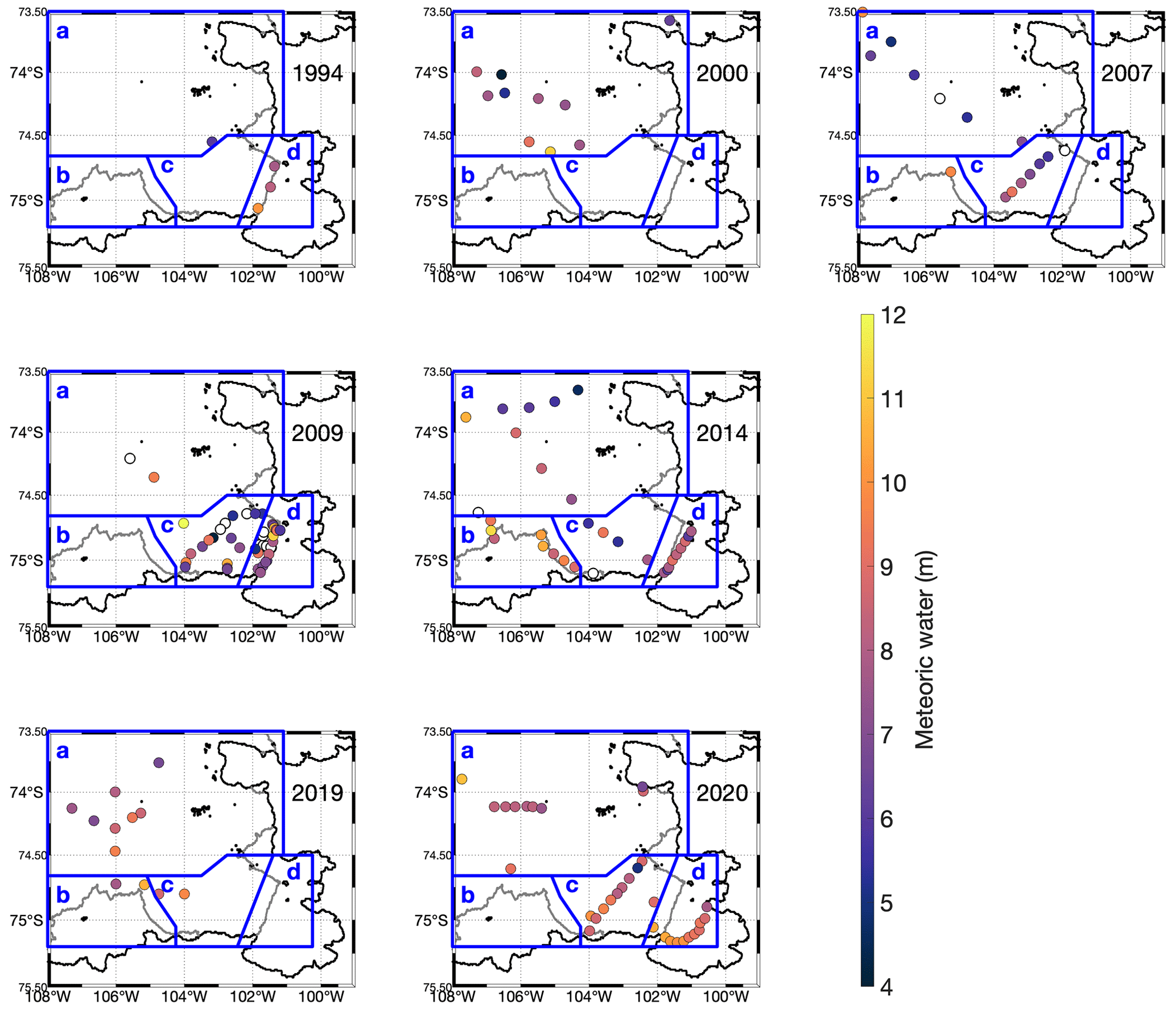
Figure A4 Sampling locations and geographic group boundaries for all years. Dot colors show the meteoric water column inventory at individual stations; outlines show geographic groupings of stations for geographic sensitivity analysis. Some locations provided only partial column inventories. White dots show stations where only one or two depths were collected.

Table A4 Results of the geographic grouping sensitivity analysis. mCDW is defined as the δ¹⁸O value at the salinity maximum falling on the linear regression of all salinity–δ¹⁸O measurements deeper than 200 m for each group of stations; meteoric water δ¹⁸O is defined as the zero-salinity intercept on that same line. Uncertainty in mCDW δ¹⁸O is represented by the 68 % prediction interval (1σ) at the salinity maximum (∼1σ), and uncertainty in salinity is the result of the randomization spatial sensitivity analysis as well as variation from the perturbation of observations by analytical precision. Average meteoric water inventory is the depth integration of the Gaussian fit of all calculated meteoric water fractions within each group, with uncertainty represented as the standard deviation in meteoric water fractions achieved using 10 000 Monte Carlo simulations perturbing the observations and endpoints by associated analytical and environmental uncertainty (Table A2). For each group of stations, mCDW and meteoric water end-members used in meteoric water calculations are defined using only those data.

mCDW (as defined in Appendix A1) exhibits little geographic sensitivity. In all years, mCDW salinity varied by less than observed seasonal variation (0.01 g kg⁻¹; Mallett et al., 2018) and δ¹⁸O exhibited less variation than that associated with instrumental precision.

The meteoric water δ¹⁸O fingerprint calculated for different geographic groupings each year is not geographically sensitive – as would be expected with deep meteoric water (basal meltwater) with a single source. In 2009, Group “a” rendered a significantly different meteoric water end-member, but this number is based on data from just four samples (three from >200 m); given the data limitations and the sample quality issues for 2009, it is unlikely that the $-\mathrm{43.7}\pm \mathrm{4.8}\mathrm{‰}$ end-member is representative.

In general, the meteoric water column inventories appear insensitive to geographic groupings. The exceptions are Group “a” in 1994 and 2009 and Group “b” in 2007, 2014, and 2019. In 1994, Group “a” contains only a single station in 1994 (eight samples) and only four samples (two stations) in 2009. Group “b” consists of those samples collected alongside TIS – locations likely to be dominated by meltwater originating from beneath PIIS (Wåhlin et al., 2021). Surprisingly, given the small number of samples collected near TIS in 2007 and 2019, the meteoric water inventories from Group “b” stations are consistent.

A4 The impact of precipitation on meteoric water inventories

Precipitation collected at Halley Bay (75.58^∘ S, 20.56^∘ W; 30 m elevation) has an average composition of $-\mathrm{22.0}\pm \mathrm{5.6}\mathrm{‰}$, while that collected at Rothera Point (67.57^∘ S, 68.13^∘ W; 5 m elevation) has an average composition of $-\mathrm{13.5}\pm \mathrm{3.4}\mathrm{‰}$, and precipitation collected at Vernadsky (65.08^∘ S, 63.98^∘ W; 20 m elevation) has an average composition of $-\mathrm{10.2}\pm \mathrm{3.0}\mathrm{‰}$ (IAEA/WMO, 2024).

Sea level precipitation collected from the field site during NBP19-01 had ¹⁸O values of $\sim -\mathrm{15}\mathrm{‰}$, consistent with expected local values from other studies (Gat and Gonfiantini, 1981; Ingraham, 1998; Noone and Simmonds, 2002; Masson-Delmotte et al., 2008). This region of the Amundsen Sea receives ∼0.5 m water equivalent of precipitation per year (Donat-Magnin et al., 2021), and mCDW on the shelf has a residence time of ∼2 years (Tamsitt et al., 2021). We recalculated water column meteoric water inventories assuming 1 m (2 full years) of local precipitation (−15 ‰ δ¹⁸O) in the upper 200 m of the water column at the time of sampling.

We find that adding 1 m of precipitation to the water column decreases the amount of meteoric water (as defined using the zero-salinity intercepts; Fig. 2) by an average of 0.55±0.01 m and decreases sea ice melt by an average of 0.57±0.03 m (Table A5). These results suggest that even with 2 years' worth of precipitation present in the water column at the time of sampling, the calculated meteoric water inventory could consist of >87 % glacial meltwater.

Table A5 Impact of precipitation on the total meteoric water column inventory. The mean meteoric water inventory is the integrated mean meteoric water content between the surface and 800 m. The upper water column will include meteoric water from both precipitation and GMW introduced at depth and mixed upward. The three rightmost columns in the table show the impact (on meteoric and sea ice meltwater column inventories) of recalculating column inventories (meteoric water $\sim -\mathrm{30}\mathrm{‰}$ δ¹⁸O; Table 2) assuming 2 years of precipitation ($\sim -\mathrm{15}\mathrm{‰}$ δ¹⁸O) in the water column at the time of sampling.

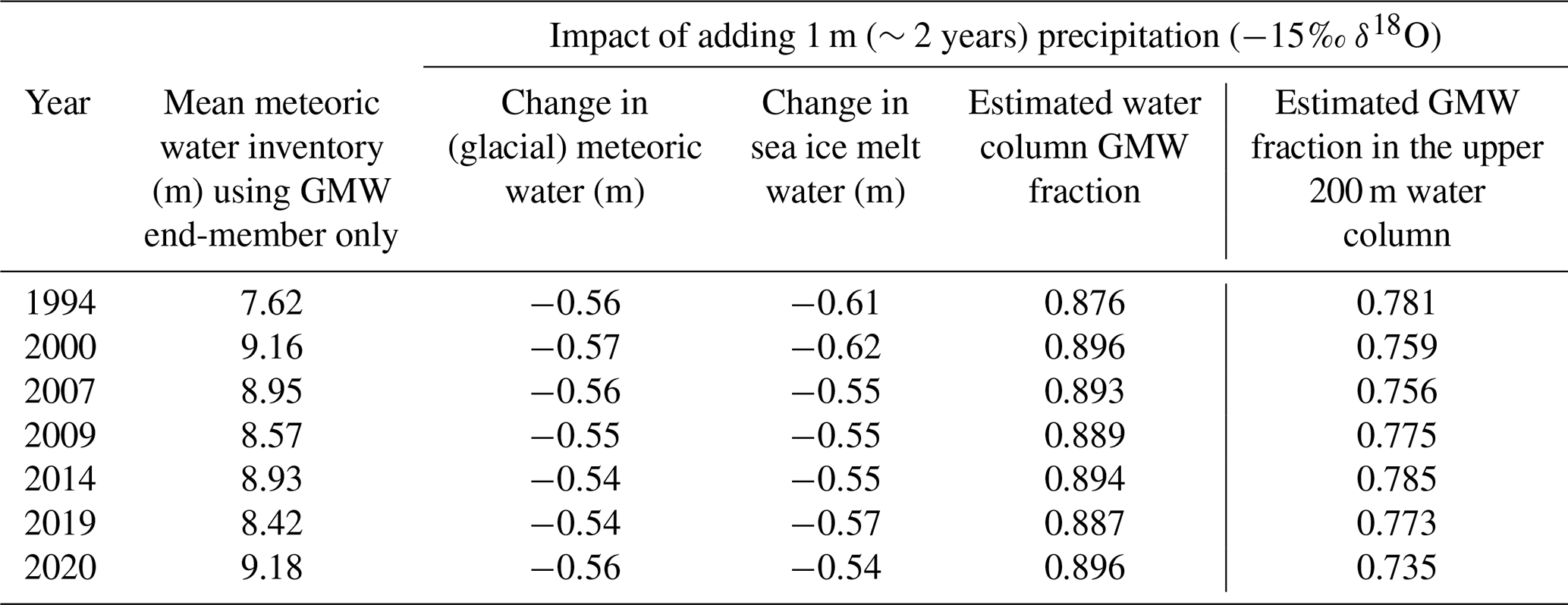
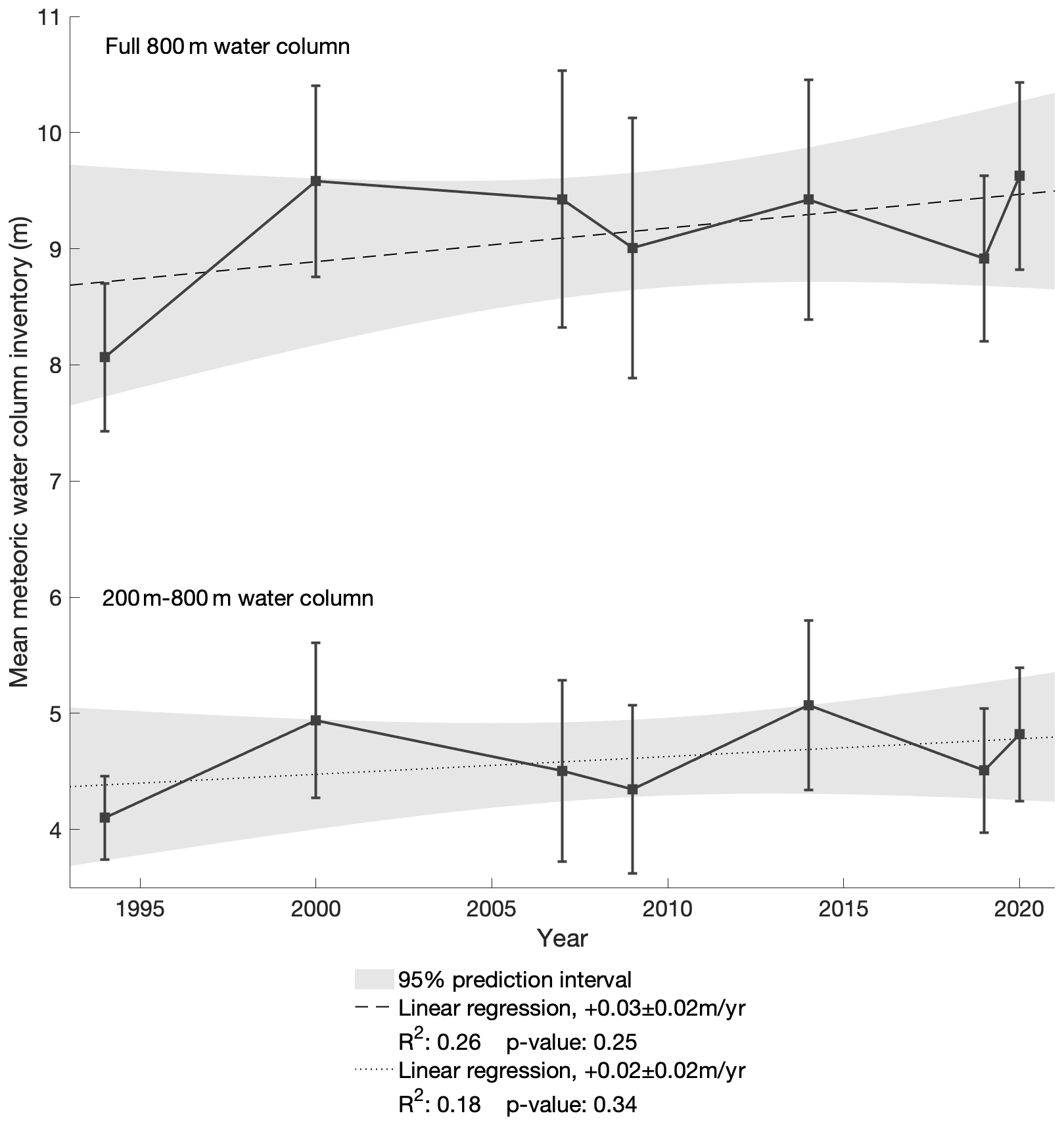
Figure A5 Mean meteoric column inventory for each sampled year. Points represent the depth-integrated meltwater volume from the Gaussian process fit (gray lines in Fig. 3) between 200 and 800 m depth. Error bars show the uncertainty in the mean meteoric water column inventory associated with analytical precision and environmental variability (Sect. 2.2). The relative year-to-year inventories here show the same general empirical trend (within uncertainty) as Fig. 5. The year 2014 shows the highest sub-200 m meteoric water content, owing to sampling immediately alongside TIS – directly in the pathway of glacial meltwater from PIIS (Wåhlin et al., 2021).

Figure A5 and Table A6 show a comparison of the yearly inventories in the total water column vs. the water column deeper than 200 m. Both the full and partial water columns show the same relative trend in meteoric water content, indicating that the observed variability is not an effect of interannual variability in precipitation.

Table A6 Relative fractions of the yearly meteoric water inventory in the 800 m and 200–800 m water columns. Reported column inventories are the depth integration of the Gaussian fit of all measurements in the field area between the specified depths. The relative fraction is the normalized relative volume of the average inventory from year to year.

A5 Sea ice melt and mCDW fractions

A5.1 Sea ice melt

Figure A6 shows the net sea ice meltwater column inventories in all sample locations. In locations where integrated sea ice melt fractions are negative, net sea ice formation at the time of sampling is indicated.

In 2007, 2009, and 2014, positive ice melt fractions >200 m likely resulted from samples subject to evaporation before analysis. Evaporation leads to positive fractionation of seawater δ¹⁸O, leading to a less depleted δ¹⁸O observation at time of analysis; less depleted δ¹⁸O relative to salinities fresher than mCDW will be interpreted by the three-end-member mixing model as sea ice melt. The stratification in this region makes it unlikely that there are significant sea ice melt fractions below 200 m. As with the δ¹⁸O–salinity (Fig. 2) and meteoric water depth (Fig. 3) plots, 1994, 2000, 2019, and 2020 exhibit the tightest distribution, suggesting higher-quality data. Gray lines show the Gaussian process fit, and points are shaded to show sample δ¹⁸O.

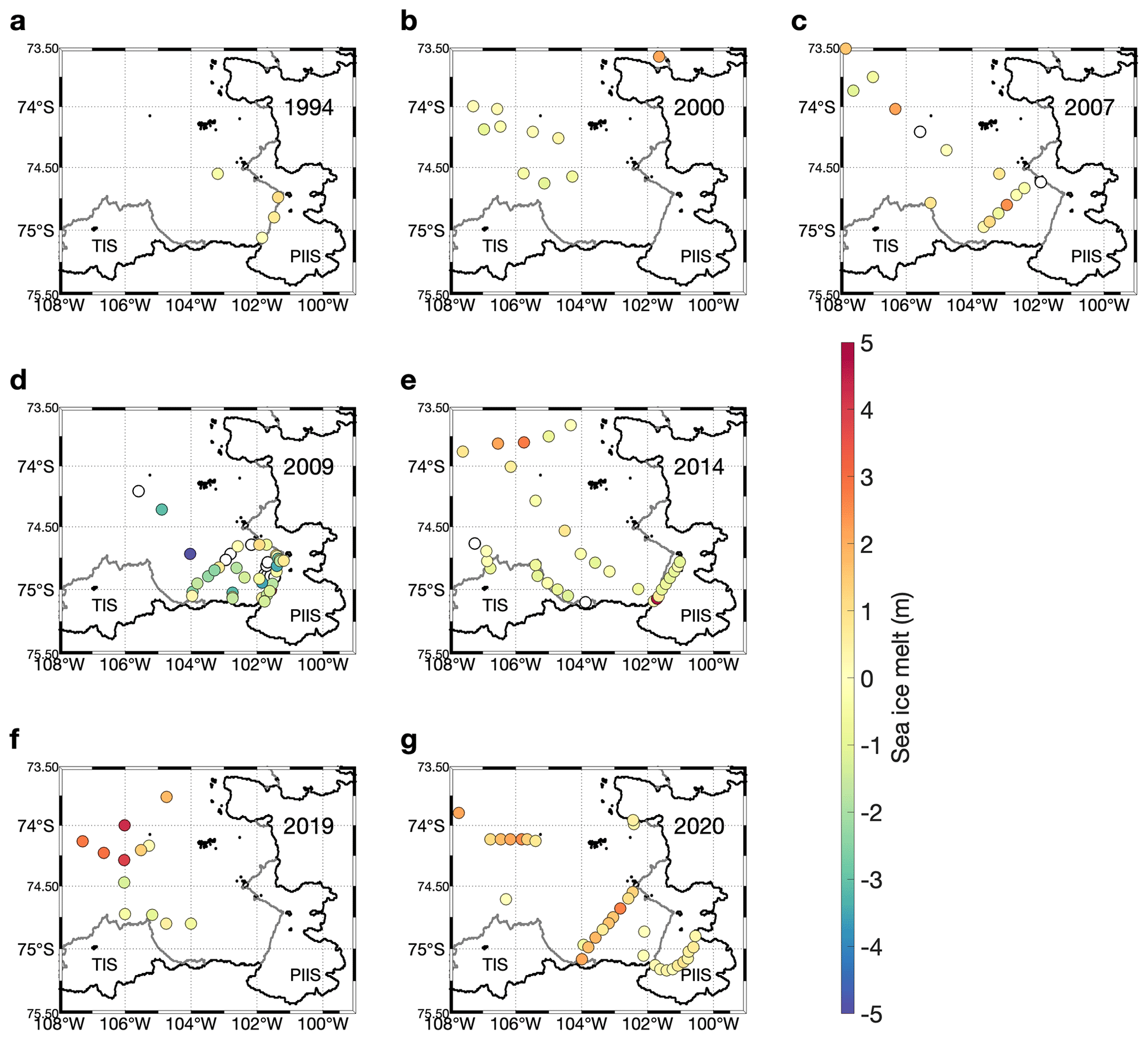
Figure A6 Integrated sea ice melt fractions at sampling locations each year. Negative sea ice melt fractions indicate areas of net sea ice formation. Stations with partial water column sampling show only partial inventories. White dots with black outlines are stations where only one or two depths were sampled (2007, 2009, and 2014). Years with greater sea ice melt (2007 and 2020) than formation show greater divergence from the mCDW–GMW mixing line in surface waters (Fig. 2).

A5.2 mCDW fractions

Waters deeper than ∼800 m are comprised of pure mCDW; moving toward the surface, meteoric freshwater from basal melt is introduced starting at ∼700 m. The near-surface waters are rich in meteoric water and/or sea ice melt, and they are comprised of >92 % mCDW (Fig. A7).

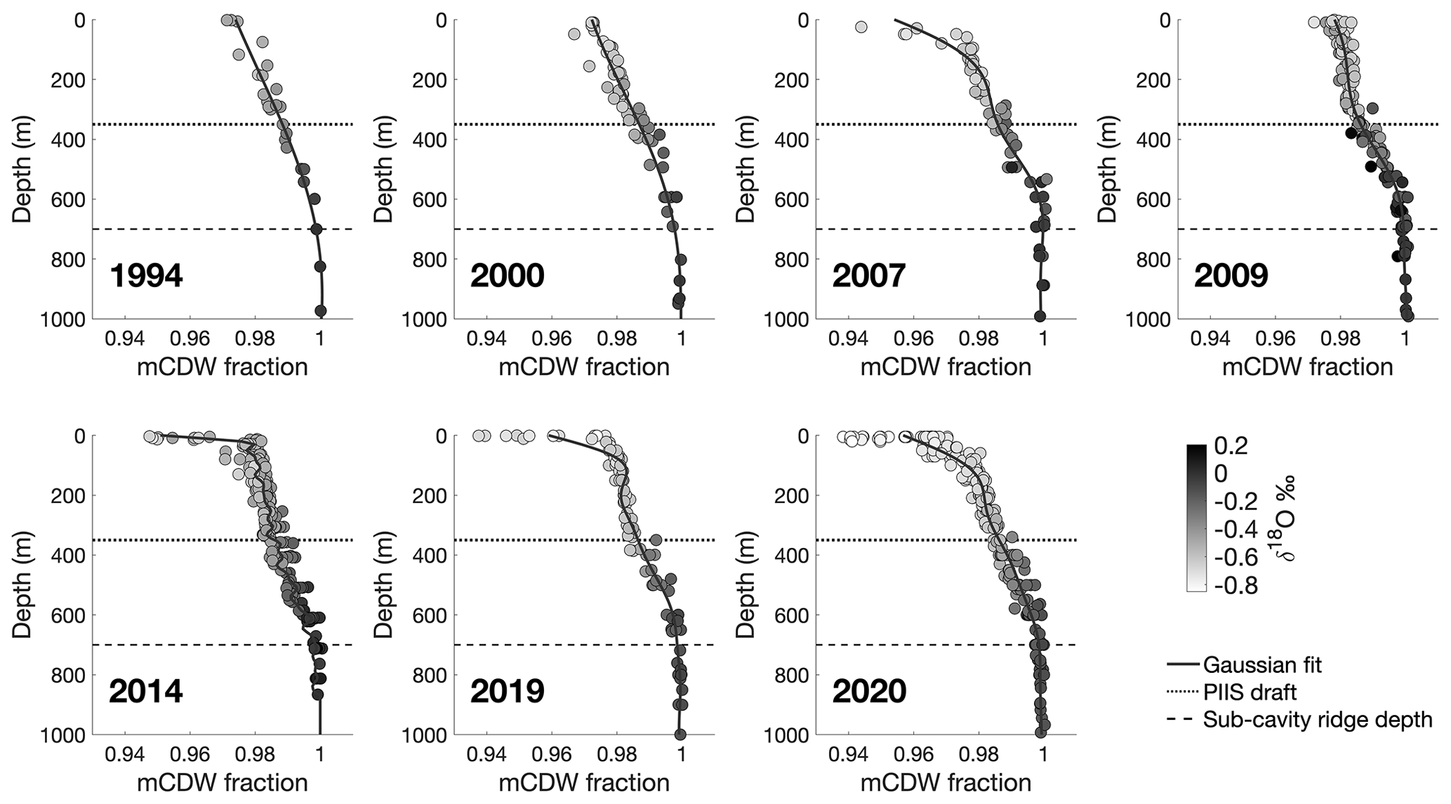
Figure A7 mCDW fractions vs. depth. Calculated mCDW fractions using salinity and δ¹⁸O measurements in the three-end-member mixing model. Shading of dots indicates the measured δ¹⁸O of that sample. Deep waters (>800 m) characterize relatively unadulterated mCDW, while near-surface waters contain the highest concentrations of sea ice melt and meteoric water. Dotted and dashed horizontal lines show the depth of the PIIS draft and the depth of the PIIS sub-cavity ridge, respectively.

Table A7 mCDW column inventories and uncertainty. Mean sea ice melt column inventories are produced by depth integration of the Gaussian process fit (gray lines Fig. A7) between the surface and 800 m. Uncertainty is described in Appendix A3.

A6 The 2009 sample quality control

A subset of the samples for 2009 were analyzed on an IRMS in 2010, while the remainder were stored until a 2020 CRDS analysis. At the latter time, 56 % of the samples analyzed contained an unknown, clear, needle-shaped precipitate. Several bottles also had a lower-than-expected sample volume, suggesting evaporation, which would likely have altered the δ¹⁸O content via isotopic fractionation. Several steps were taken to ensure the quality of samples analyzed after a decade in storage.

A6.1 Scanning electron microscopy (SEM) and energy dispersive X-ray spectroscopy (EDS) analysis of precipitate

Samples of the precipitate were extracted from multiple sample bottles and analyzed using a scanning electron microscope, equipped with a FEI Magellan 400 XHR SEM with Bruker QUANTAX XFlash 6-60 silicon drift detector (SDD) EDS detector, at the Stanford Nano Shared Facilities (SNSF). Peaks were observed at the spectra associated with Mg, Si, and O, indicating the precipitate is likely some form of magnesium silicate hydroxide (Mg₃Si₂O₅(OH)₄) or magnesium silicate hydrate (Mg₂Si₃O₈ | H₂O). Si(OH)₄ is the simplest soluble form of silica and is found universally in seawater at low concentrations (Belton et al., 2012). The maximum amount of silicate that could be expected in this area of the ocean is ∼100 µmol kg⁻¹ (Rubin et al., 1998). In this case, even if the entire 100 µmol kg⁻¹ of Si was drawn down to 0, solely into a magnesium silicate, with a very high fractionation factor, e.g., the −40 ‰ reported for diatoms (Leclerc and Labeyrie, 1987), the greatest effect on a sample would be 0.0003 ‰ – well below the analytical precision of the CRDS (0.025 ‰) or IRMS (0.04 ‰). Therefore, it is highly unlikely that the precipitate contributed a detectable fractionation or alteration of seawater δ¹⁸O in our samples.

A6.2 Quality control for evaporation

In all years, the bulk of the δ¹⁸O data fall in a broadly predictable pattern: less depleted at depths below ∼600 m and more depleted near the surface. Values >2 standard deviations from this pattern denote samples that were likely subject to significant evaporation (Fig. A8)

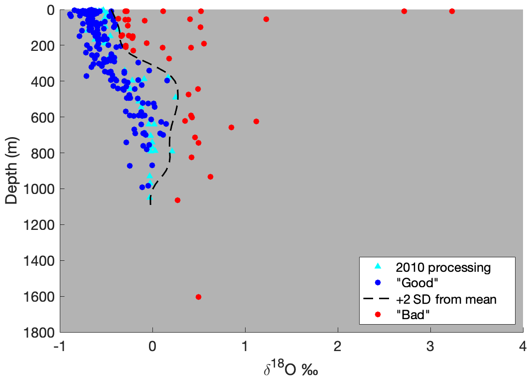
Figure A8 δ¹⁸O vs. depth for all 2009 samples, coded for likelihood of evaporation. The dashed line represents +2 standard deviations from a moving depth-averaged δ¹⁸O based on the 2010 processing, beyond which the results are unacceptable. Archivable data can be found at https://doi.org/10.25740/zf704jg7109 (Hennig et al., 2023).

As a secondary check, the δ¹⁸O of all samples was plotted vs. depth with a qualitative indicator of the amount of precipitate found in the sample vial (Fig. A9) to see if any patterns emerged compared to that of depth-comparable samples processed in 2010. No clear trend was evident.

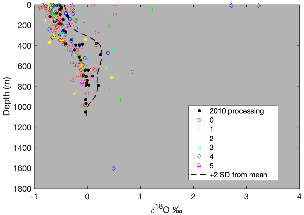
Figure A9 δ¹⁸O vs. depth of all 2009 samples, coded by the amount of precipitate present. Each bottle was graded by eye based on the volume of precipitate present, with 0 being no precipitate present and 5 being the most precipitate present. As for Fig. A8, the dashed line represents +2 standard deviations from the mean δ¹⁸O at each depth.

Evaporation is accompanied by isotopic fractionation, with H${}_{\mathrm{2}}^{\mathrm{16}}$O evaporating preferentially, leaving the remaining liquid relatively enriched in H${}_{\mathrm{2}}^{\mathrm{18}}$O. Evaporation also increases the salinity, and thus density, of the remaining sample. We measured the density of each seawater sample five times using a calibrated 1 mL pipet and milligram balance. The theoretical density of each sample was calculated from its associated CTD salinity and temperature. Differences between measured and theoretical densities for each sample are plotted in Fig. A10.

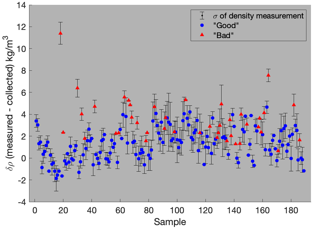
Figure A10 Difference in measured density vs. theoretical density for each 2009 sample analyzed in 2020. Theoretical density is based on CTD salinity at each sample location, whereas measured density is calculated from 1 mL sample aliquots weighed on a milligram scale, with sample coding as in Fig. A8. Error bars represent the standard deviation of replicates for each measurement.

While a few samples show clear evidence of evaporation, and correspondingly high δ¹⁸O values, most show less-obvious density anomalies, exposing the limitations of our scale accuracy at that level. A total of 75 % of the samples measured showed a higher-than-expected density, whereas 25 % measured a lower-than-expected value. Figure A10 displays a significant overlap in measured density space between samples previously identified as “good” or “bad” (Fig. A8). Figure A10 shows that there are no samples flagged as compromised (bad) from our earlier depth-based analysis with a δρ greater than 1.3 kg m⁻³. At an aggressive first pass, we removed all sample data with a δρ greater than 1.3 kg m⁻³ and looked at each hydrocast profile individually, using the remaining data. Excluded samples flagged as good were returned to the dataset, and individual profiles were re-scrutinized to check for any qualitative anomalies.

A6.3 Conclusion and final 2009 sample inclusion

While it is very unlikely that the precipitate changed sample values, some samples do appear to have been subject to evaporation. The inclusion of all samples flagged as good does not qualitatively change our analyses when compared with the data processed in 2010. We exclude the 41 samples initially flagged as bad (Fig. A8) and retain the remaining 148 flagged as good.

A7 CRDS and IRMS cross-calibration

We processed 100 samples from 2019 and 2020 concurrently using the Picarro L2140-i CRDS and a Finnigan MAT252 IRMS (Fig. A11) with CO₂ equilibration (Epstein and Mayeda, 1953). Both instruments were independently calibrated using the VSMOW, Standard Light Antarctic Precipitation (SLAP), and Greenland Ice Sheet Precipitation (GISP) international standards, and all samples were run in duplicate. The data from both machines were comparable, with the Picarro achieving a precision of 0.02 ‰, and the IRMS achieving a precision of 0.03 ‰ on replicates. The offset between CRDS and IRMS data averaged −0.02 ‰, with the CRDS data being more negative. As the offset between the two machines was less than either instrument's precision, data from the CRDS were used in their unadjusted form. Values reported for the CRDS are the average of six individual injections/measurements from each vial; reported precision is based on the standard deviation between multiple six-injection averages from replicate analyses, separated by days, weeks, or months.

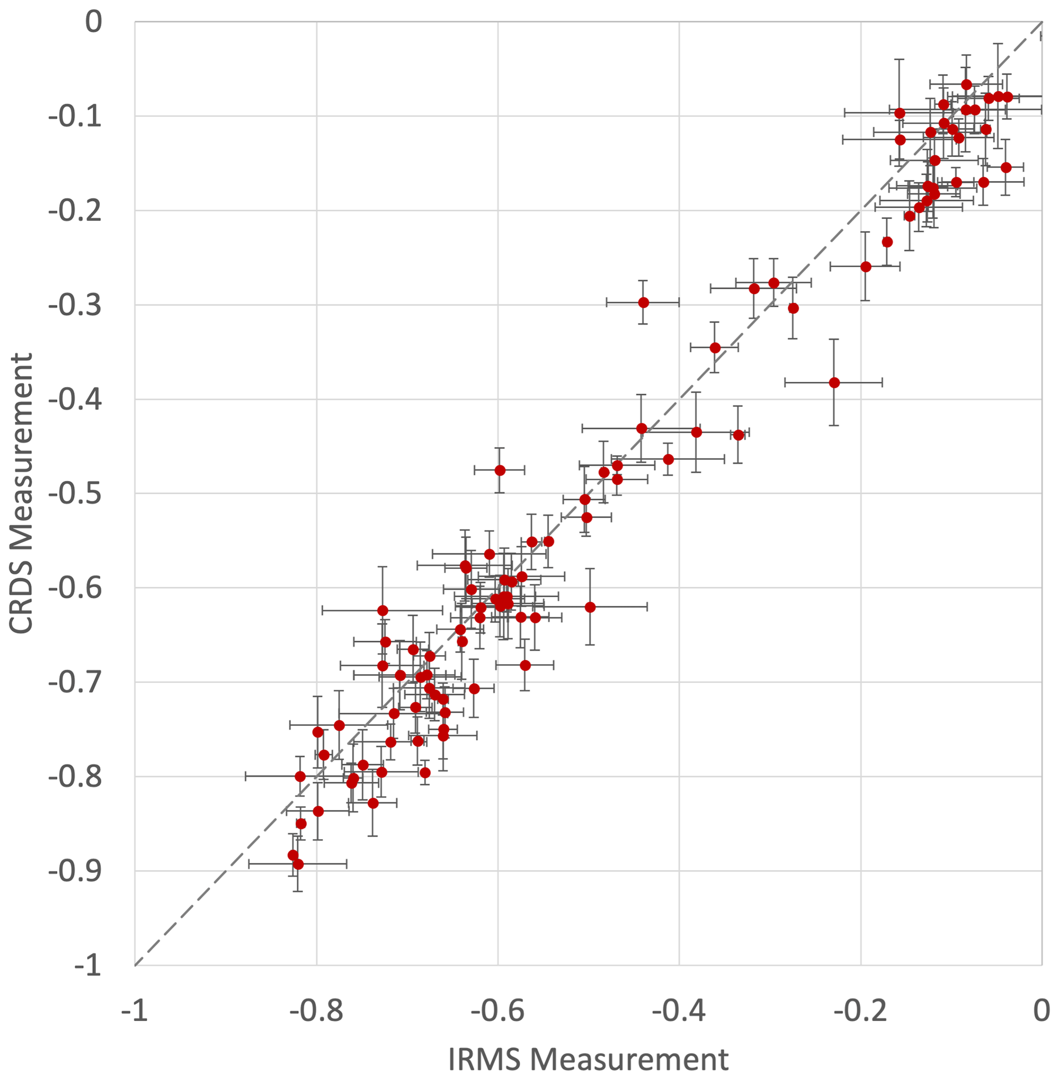
Figure A11 The 101 seawater δ¹⁸O samples collected in 2019 and 2020 analyzed with both CRDS and IRMS. Each point represents the value obtained by measuring the same sample on the IRMS (x axis, ‰ δ¹⁸O) and the CRDS (y axis, ‰ δ¹⁸O). Error bars represent the corresponding standard deviation of the IRMS and CRDS measurements. The dashed gray line is a 1:1 slope.

A8 CRDS methods

A total of 570 of the isotope samples for this study (all samples from 2019 and 2020 as well as portions from 2007 and 2009) were run on a Picarro L2140-i CRDS system, rather than a traditional IRMS. Using this system, we were able to achieve an average precision of <0.02 ‰ for multiple-replicate analyses.

Samples were collected in 10 or 30 mL glass serum vials (Fisher Scientific part no. 06-406D/06-406F) and sealed with rubber stoppers (Fisher Scientific part no. 06-406-11B) and aluminum seals (Fisher Scientific part no. 06-406-15).

Sample vials should be filled to just below the “neck” (narrowest part). Minimizing the headspace of the vial is important for minimizing evaporation; however, it is important to leave some headspace to allow for expansion/contraction of the sample (if collecting samples larger than 30 mL, slightly more headspace should be left, with 250 mL vials being filled to about halfway up the “shoulder” before the neck). When sealing serum vials with rubber stoppers and aluminum seals, it is important that the tops of the aluminum seals are crimped tightly but remain flat after crimping/capping. An upward “buckling” of the aluminum seal indicates over-crimping and will produce an inferior seal.

Internal laboratory (Stanford Impact Labs) data show that samples can be preserved in this manner for multiple years without significant degradation, while bottles with threaded caps and PARAFILM reliably prevent sample evaporation up to the level of instrument analytical precision for no more than 1 year.

The instrument setup used was as follows:

• 10 µL syringe (Trajan part no. 002982);

• a single standard or unknown run consists of seven injections (measurements) per sample;

• sample injection volume of 2.2 µL;

• 3×5 µL rinses with fresh water from inkwell (IW) between each sample;

• 3×2.2 µL rinses with sample before first measurement of new sample or standard vial;

• rinse only between sample vials or one rinse for every seven standard or unknown injections.

Several protocols were also followed with regards to sample and instrument handling. These protocols are as follows:

• The ILS was prepared to have a δ¹⁸O value in the middle of the range expected from the unknowns (i.e., $\sim -\mathrm{0.3}\mathrm{‰}$) to minimize memory issues between samples. The IW was also filled with water of approximately this composition.

• A fresh 2 mL vial of ILS was used each day and discarded at the end of the sequence.

• Samples were pipetted from sealed 10 or 30 mL serum vials into 2 mL vials (Fisher Scientific part no. 03-391-15) for analysis on the day that they were to be analyzed. The 2 mL vials used for analysis were found to only reliably preserve sample δ¹⁸O for <1 week.

• After each sequence, the syringe was cleaned with deionized (DI) water and then rinsed thoroughly with water from the inkwell, to minimize memory and contamination issues due to residual water left in the syringe. Treated in this way, syringes can be expected to last for 1500 to 2500 injections.

• A fresh vaporizer septa (Trajan part no. 0418240) was used every day.

• ILS values were analyzed no less than every fifth unknown, and no fewer than three ILS values were measured per run.

• All data were corrected based on the slope of the ILS measurements over the course of the sequence.

• Each run began with no fewer than 10 injections from the IW, to allow the instrument to reach baseline.

• The syringe was cleaned thoroughly with DI water each day and manually rinsed with IW water prior to sequence.

• ILS was measured (seven injections) no less than once every five unknowns (seven injections each).

• ILS values were measured at least three times during each sequence – at the beginning, end, and midpoint. At least three standards were measured during each sequence.

A typical 24h sequence ran 16 unknowns. The sequence was set up as follows:

• 15 injections from the IW;

• ILS (7 injections);

• 4 unknowns (4×7 injections);

• ILS (7 injections);

• 4 unknowns (4×7 injections);

• ILS (7 injections);

• 4 unknowns (4×7 injections);

• ILS (7 injections);

• 4 unknowns (4×7 injections);

• ILS (7 injections).

Overall, this sequence consists of 162 injections, 112 of which contained salt, for a vaporizer load of ∼8.6 mg of salt per day. The instrument vaporizer was cleaned at least every 200 mg worth of salt injected. At 35 PSU (practical salinity units) and 2.2 µL injections, this is 2597 salty injections, or 371 samples at 7 injections each (∼ every 23 analytical days).

Finally, analytical data quality control was conducted in the following way:

• The first injection of each sample was discarded, to minimize instrument memory issues.

• If the standard deviation of the remaining six injections was >0.04 ‰, up to one outlier could be removed. Any samples where the standard deviation of measured values was still >0.04 ‰ were rerun the following day from the same vial, using the same septa.

• If a rerun was possible the following day, the vial septa was replaced with a new one.

• Data from each hydrocast were inspected as a group. Any samples that appeared inconsistent with the rest of the hydrocast (e.g., with regards to salinity or neighboring δ¹⁸O values) were rerun. If the rerun occurred within 1 week of the initial run, the same vial was used; otherwise, a fresh aliquot of sample was drawn from the resealed serum vial.