In situ estimation of ice crystal properties at the South Pole using LED calibration data from the IceCube Neutrino Observatory

The IceCube Neutrino Observatory instruments about 1 km³ of deep, glacial ice at the geographic South Pole. It uses 5160 photomultipliers to detect Cherenkov light emitted by charged relativistic particles. An unexpected light propagation effect observed by the experiment is an anisotropic attenuation, which is aligned with the local flow direction of the ice. We examine birefringent light propagation through the polycrystalline ice microstructure as a possible explanation for this effect. The predictions of a first-principles model developed for this purpose, in particular curved light trajectories resulting from asymmetric diffusion, provide a qualitatively good match to the main features of the data. This in turn allows us to deduce ice crystal properties. Since the wavelength of the detected light is short compared to the crystal size, these crystal properties include not only the crystal orientation fabric, but also the average crystal size and shape, as a function of depth. By adding small empirical corrections to this first-principles model, a quantitatively accurate description of the optical properties of the IceCube glacial ice is obtained. In this paper, we present the experimental signature of ice optical anisotropy observed in IceCube light-emitting diode (LED) calibration data, the theory and parameterization of the birefringence effect, the fitting procedures of these parameterizations to experimental data, and the inferred crystal properties.

1 Introduction

The 2021 IPCC report (Intergovernmental Panel on Climate Change, 2021) highlights the need to understand the dynamics of ice sheets in order to predict their contribution to sea level rise in a changing climate. Ice flows under its own weight, either through basal sliding or through plastic deformation, which is mediated by the deformations of individual grains as well as interactions between grains (e.g., Cuffey, 2010). The viscosity of an individual ice crystal strongly depends on the direction of the applied strain, and it will most readily deform as shear is applied orthogonal to the c axis (crystal symmetry axis, normal to the hexagonal basal planes), leading to slip of the individual basal planes (e.g., McConnel, 1891; Hobbs, 2010; Petrenko and Whitworth, 2002). In polycrystalline ice subjected to strain, the crystals may undergo lattice rotation or recrystallization, both of which result in non-isotropic c-axis distributions and a bulk anisotropic viscosity (e.g., Faria et al., 2014b).

In this work we only consider scenarios in which the c axes are distributed isotropically (uniform fabric), are aligned in a single direction (single-pole fabric), or lie in a plane (girdle fabric). The latter is of primary importance for the studied ice.

The crystal orientation fabric is experimentally most commonly observed through the use of polarized-light microscopy on thin sections of ice core samples (e.g., Alley, 1988; Wilson et al., 2003; Langway, 1958; Wilen et al., 2003).

The average crystal size and elongation can also be quantified directly through microscopy (e.g., Fitzpatrick et al., 2014).

While ice core analysis uniquely delivers ground-truth information, it is limited by its small sampling volume and often unable to resolve the absolute direction of fabric orientation as the core orientation is not preserved in the drilling process (e.g., Westhoff et al., 2021). Volumetric quantities such as grain volumes and shapes are generally not directly accessible through the commonly employed techniques. Grain sizes and elongations evaluated through the microscopy of thin slices cut from ice cores in turn often depend on the sample plane.

Ice fabric can be imaged not only in ice cores. It also leads to a directionality in the propagation of sound and electromagnetic radiation. The mechanical anisotropy of ice results in a fabric-dependent speed of sound, as has, for example, been measured using a sonic logger in boreholes (Kluskiewicz et al., 2017). Ice crystals also are a birefringent material such that any incoming electromagnetic radiation is separated into an ordinary and extraordinary ray of perpendicular polarizations with respect to the c axis and which propagate with different refractive indices. Today this is primarily employed by polarimetric radar systems to infer fabric properties (e.g., Fujita et al., 2006; Matsuoka et al., 2003; Jordan et al., 2019; Young et al., 2021) through periodic power anomalies detected as a result of the direction and polarization-dependent delay in the propagation of radio waves.

Recently, as part of ice calibration measurements for the IceCube Neutrino Observatory (Aartsen et al., 2017), Chirkin (2013d) described the observation of an “ice optical anisotropy”. At receivers 125 m away from isotropic 400 nm emitters, about twice as much light is observed for emitter–receiver pairs oriented along the glacial flow axis versus orthogonal to the flow axis (see Fig. 4). The effect was originally modeled as a direction-dependent modification to impurity-induced Mie scattering quantities, either through a modification of the scattering function as proposed by Chirkin (2013d) or through the introduction of a direction-dependent absorption as introduced by Rongen (2019). As also shown by Rongen (2019), both parameterizations lack a thorough theoretical justification and resulted in an incomplete description of the IceCube data (see Fig. 6).

First attempts to attribute the observed effect not to Mie scattering but to the ice-intrinsic birefringence have been made by Chirkin and Rongen (2020). Here the optical anisotropy results from the cumulative diffusion that a beam of light experiences as it is refracted or reflected on many grain boundaries in a birefringent polycrystal with a preferential c-axis distribution. The wavelength of ∼400 nm employed in the IceCube calibration studies is significantly smaller than the average grain size, which is expected to be on the millimeter scale. Thus, the spacing of grain boundaries and the distribution of encountered grain boundary orientations, both of which are a function of the average grain shape, must be accounted for in addition to the fabric.

In this scenario the diffusion is found to be strongest when photons initially propagate along the ice flow axis and smallest when initially propagating orthogonal to the flow axis. In addition photons are, on average, deflected towards the flow axis. The deflection per unit distance increases for stronger girdle fabrics, a larger average crystal elongation, or a smaller average crystal size. For crystal configurations and/or realizations where the deflection outweighs the additional diffusion along the flow axis compared to the diffusion along the orthogonal direction, the photon flux along the flow axis will increase with distance compared to the photon flux along the orthogonal axis. This interplay between diffusion and deflection leaves a unique imprint in the spatial and temporal light signatures recorded by IceCube. Due to computational limitations, a grain-resolving anisotropic optical model has been parameterized by Abbasi et al. (2021) using diffusion functions. These functions in turn have been applied as an extension to the existing homogeneous ice optical simulation. These simulations, assuming different ice crystal realizations, have then been compared to LED flasher data, which partially constrain the crystal fabric, size, and elongation.

Work on this model has so far been performed and proceedings published (Chirkin, 2013d; Chirkin and Rongen, 2020; Abbasi et al., 2021) in the context of detector calibration for the measurements performed by IceCube. With this paper we will summarize the full extent of past and ongoing modeling of the ice optical anisotropy to a geophysical audience for the first time. The described measurements may be unique to IceCube and thus not easily adopted as a tool in glaciology. Nevertheless we believe that they yield an interesting complementary view on ice physical properties and through comparison to ice core data, in particular from SPC14 (Casey et al., 2014) drilled ∼1 km from the IceCube array, will be informative for the modeling of ice dynamics.

This paper has the following structure: Sect. 2 introduces the IceCube Neutrino Observatory (Sects. 2.1 and 2.2) and how it employs ice as a detection medium (Sect. 2.3). Section 3 describes the properties of the LED calibration data used in this study (Sect. 3.1), explains the photon propagation software used to generate simulated data (Sect. 3.2), and details the likelihood analysis comparing simulated to experimental data in order to infer ice properties (Sect. 3.3). The state of the isotropic, layered model used to describe the ice optical properties prior to the discovery of the ice optical anisotropy is briefly reviewed in Sect. 3.4. The experimental signature of the ice optical anisotropy (Sect. 4.1) and early modeling attempts (Sect. 4.3) are summarized in Sect. 4. The newly developed model to account for the ice optical anisotropy based on the ice-intrinsic birefringence is described starting with Sect. 5. Section 5.2 explains the electromagnetic theory governing the birefringence in polycrystals, while Sect. 5.3 introduces a software package to simulate the resulting diffusion patterns. Section 5.4 compares the experimental signatures and conceptual understanding of the underlying optics to birefringence observations in radar sounding, a field most readers are probably more familiar with. Section 6 explains how the diffusion patterns are applied in the IceCube photon propagation simulation (Sects. 6.1 and 6.2) and how crystal properties have been inferred (Sect. 6.3). The resulting ice optical model is described in Sect. 7. Section 8 discusses shortcomings of the model as well as future measurements in upcoming IceCube extensions and through drill-hole logging.

2 The IceCube Neutrino Observatory

2.1 Scientific context: neutrino astronomy

The IceCube Neutrino Observatory operates within the context of astroparticle physics and multi-messenger astronomy. While astronomy is most commonly associated with the observation of the universe in visible light, today the entire electromagnetic spectrum ranging from radio waves to hard X-rays and ultrahigh-energy gamma rays is exploited, with each spectral range giving a complementary insight. Infrared radiation, for example, is only weakly attenuated by interstellar dust (e.g., Li and Draine, 2001), allowing for the imaging of objects otherwise obscured by dust clouds.

In addition to photons, the quanta of light, other stable messenger particles are also observed. Most prominently cosmic rays, primarily protons, have now been found at energies exceeding 5×10¹⁹ eV, the equivalent of roughly 8 J per particle (Aab et al., 2020). While these ultrahigh-energy cosmic rays offer the promise to probe the highest-energy processes in the universe, they are deflected by magnetic fields along their journey from source to detection (e.g., Aartsen et al., 2015). Thus their arrival directions at Earth cannot be easily traced to their origins, making the identification of the sources of high-energy cosmic rays one of the biggest challenges in astroparticle physics.

Associated with the production of high-energy protons, one expects the production of high-energy neutrinos, or astrophysical neutrinos (e.g., Margolis et al., 1978). These are electrically neutral, elementary particles belonging to the family of leptons (as counterparts to electrons, muons, and taus). As they are electrically neutral, they are not deflected in magnetic fields and thus point back to their point of origin. Additionally they only interact through the weak force and as a result can traverse vast astronomical distances without their flux being significantly attenuated. While these properties ensure that neutrinos carry unbiased information about the highest-energy regions of the universe, these same properties also make them exceptionally hard to detect, requiring cubic-kilometer-scale detectors to intercept a few dozen astrophysical neutrinos per year (e.g., Markov, 1960). Detectors of this scale can only be built into natural media such as ocean water or glacial ice, which need to be characterized in situ as presented here.

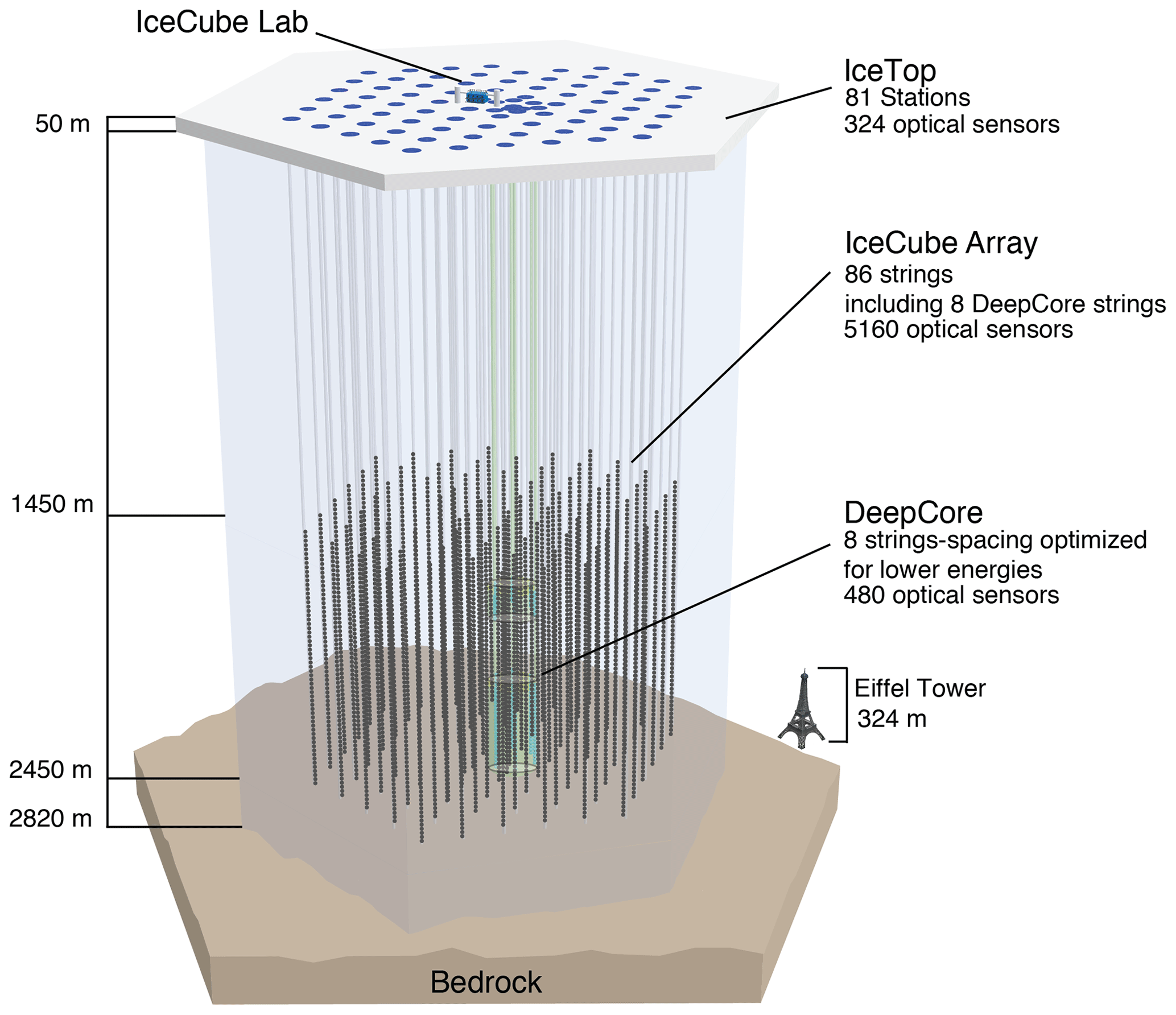
Figure 1 Overview of the IceCube detector. The 86 cables of the deep in-ice array, called strings, are indicated as gray lines, with black dots for the 60 DOMs per string. The lateral spacing of the strings is ∼125 m with a vertical spacing between DOMs of 17 m. A central part of the array, called DeepCore, is more densely instrumented. The detector is capped by a surface detector, aimed at cosmic ray physics, called IceTop. Figure credit: IceCube.

2.2 The detector

The IceCube Neutrino Observatory (Aartsen et al., 2017) has, among other science goals, been built to explore the cosmos using high-energy astrophysical neutrinos. Located about 1 km from the geographic South Pole, it is logistically supported by the Amundsen–Scott South Pole Station. IceCube features a surface detector, called IceTop, as well as the deep in-ice array of interest here, which consists of 5160 optical sensors instrumenting a 1 km³ volume of ice at depths of 1450 m to 2450 m. The instrumentation layout is shown in Fig. 1. Each sensor, called a digital optical module (DOM) (Stokstad, 2005; Abbasi et al., 2010, 2009), is equipped with a 10 in. photomultiplier tube sensitive to light between approximately 300–600 nm and all required readout electronics to be able to time-stamp the arrival time of individual photons to within 2 ns. It addition each DOM features 12 LEDs which can emit light pulses of known intensity and duration into the ice and which are used to calibrate the optical properties of the instrumented ice, as detailed in this paper. Construction took 6 years, with 86 holes of 60 cm diameter being drilled using hot-water drilling (Benson et al., 2014). Cables called “strings” were instrumented with 60 DOMs each and deployed in the boreholes.

The top 1450 m was left without instrumentation because of the strongly scattering ice that exists in this region. The depth where most bubbles have converted to air hydrates was determined to be roughly 1350 m by the predecessor experiment AMANDA (Ackermann et al., 2006).

Upon a neutrino interaction in the ice, charged particles with relativistic velocities are created, which emit blue light along their path through a process called Cherenkov radiation (Cherenkov, 1937). A small fraction of this light, after propagating through the ice, reaches some of the sensors and is detected. Reconstruction of the particle properties, namely energy and direction, relies on a precise understanding of the optical properties of the instrumented ice. Generally the particle energy is proportional to the amount of detected light, while the arrival direction is inferred from the geometric deposition of the light as well as its timing information (Aartsen et al., 2013d).

Since its completion in 2010, the IceCube detector has been in continuous operation with an up-time exceeding 99 %. On average around 2000 particle events are detected and reconstructed per second, with the vast majority of these being particle showers induced by cosmic rays striking Earth's atmosphere and only a vanishing fraction (approximately hundreds per year) being astrophysical neutrinos. Using IceCube data, a wide range of results have been obtained. Those include, among others, the discovery of a high-energy astrophysical neutrino flux (Aartsen et al., 2014) and first associations of high-energy neutrinos with astrophysical objects (Aartsen et al., 2018a), competitive measurements of neutrino oscillation parameters (Aartsen et al., 2018b), and world-leading limits on possible dark-matter properties (Albert et al., 2020).

2.3 Glacial ice as an optical medium

IceCube detects individual photons that are produced through Cherenkov radiation or as emitted by the calibration LEDs. On their way from their source to a potential detection at a DOM these photons are subject to absorption and scattering in the ice, shaping both the intensity pattern in the detector and the arrival time distributions on every module.

Absorption is characterized by a wavelength-dependent λ absorption length λ_a(λ), the propagated distance at which the survival probability of a photon drops to $\mathrm{1}/e$. In contrast, scattering does not reduce the photon count but results in discrete direction changes at an average distance of λ_b(λ), the geometric scattering length. Scattering is further described by the scattering function, a probability density distribution describing the probability of deflection angles in each scattering process. Neglecting its functional form, the scattering function is described through the average deflection angle or asymmetry parameter g=〈cos θ〉. The effective scattering length λ_eff, denoting the distance at which an initially directional beam becomes diffuse independent of the scattering function, is given as (Aartsen et al., 2013c)

$$\begin{array}{}\text{(1)}& {\mathit{\lambda }}_{\mathrm{eff}}\left(\mathit{\lambda }\right)={\mathit{\lambda }}_b\left(\mathit{\lambda }\right)/\left[\mathrm{1}-g\left(\mathit{\lambda }\right)\right].\end{array}$$

As pure ice itself is only very weakly absorbing (Warren and Brandt, 2008) (and as we will see later also effectively weakly scattering), the light propagation is dominated by Mie scattering on impurities. In this scenario absorption and scattering strengths are commonly denoted by coefficients ($a=\mathrm{1}/{\mathit{\lambda }}_{\mathrm{a}}$ and $b_e=\mathrm{1}/{\mathit{\lambda }}_{\mathrm{eff}}$), which are proportional to the impurity concentration (Ackermann et al., 2006). The primary impurity constituents contributing to absorption and scattering were identified by He and Price (1998) to be mineral dust, marine salt, and acid droplets as well as soot. These constituents range from nanometer to micrometer in size, with their combined size distribution resulting in a very strong forward scattering with g≈0.95 at the relevant wavelengths around 400 nm (He and Price, 1998). The impurities have been deposited with the snow precipitation over the past 100 kyr, which was compressed into the ice that is present today at the relevant depths. The impurity composition and concentration, and thus also the optical properties, accordingly trace the global climatological conditions such as dust and aerosols in the atmosphere in the past. This stratigraphy was traced at millimeter resolution using a laser dust logger deployed down seven IceCube drill holes as described by Aartsen et al. (2013a).

While not contributing to absorption, air hydrates also contribute to scattering. Their number density is large, and their large size (Uchida et al., 2011), compared to the typical wavelengths considered, results in isotropic scattering. Yet due to the small difference in refractive index (Uchida et al., 1995) compared to ice they contribute at most a few percent to the overall scattering coefficient (He and Price, 1998). Thus, scattering on air hydrates was previously not modeled explicitly and its impact was effectively incorporated into the overall scattering coefficients. Diffusion through scattering on grain boundaries was also already quantitatively estimated by He and Price (1998) to contribute about as much as air hydrates to the overall scattering coefficient. At the time the average deflection process described in this work was not known and thus its large importance not realized. The quantitative contribution of diffusion in the polycrystal to the overall scattering coefficient as derived in this work is given in Sect. 7.

Describing the depth dependence

The detailed stratigraphy associated with the yearly layering cannot be constrained through IceCube data, nor is it needed in order to accurately describe the photon propagation over large distances exceeding tens of meters. Instead, average properties in 10 m depth increments, here called “ice layers”, are being considered. The absolute depths of these layers, such as shown in Fig. 3, are referenced to a location in the center of the surface area of the detector. At any other location in the detector the same layers are found at slightly different depths following the layer undulations as will be described in Sect. 3.4.1. Each layer is described by its dust-induced absorption and scattering coefficients at a wavelength of 400 nm. These are scaled to other wavelengths as described by Aartsen et al. (2013c).

While all parameters are in principle depth-dependent, e.g., the asymmetry factor g due to changes in the impurity composition, some are deemed constant enough to be described by a single global value or functional parameterization. These are the coefficients describing the wavelength dependence and the parameterization of the scattering function, achieved through a mixture of the Henyey–Greenstein (Henyey and Greenstein, 1941) and simplified Liu (Liu, 1994) approximations of Mie scattering, as well as its asymmetry parameters g. Thus six global parameters (three for the wavelength dependencies, one ice intrinsic absorption in the infrared, two for the scattering function – g and the mixing ratio) and about 100 layers within the instrumented volume, with individual dust-induced absorption and scattering coefficients each, are required to describe the layered ice properties.

3 Deriving ice optical properties from LED calibration data

3.1 LED calibration data

As will be described in Sect. 3.4 the absorption and effective scattering lengths encountered at IceCube depths range up to 400 and 100 m, respectively. The limited volume of the ice cores thus does not allow for a direct measurement of optical properties, even though they are able to provide information on the impurity constituents and their size distributions. To enable in situ calibration of the ice optical properties, each of the 5160 DOMs deployed in ice is equipped with 12 light-emitting diodes (LEDs) that are positioned on a “flasher” board and can emit light one at a time or in simultaneous combinations. The LEDs are placed in pairs at 60^∘ increments in azimuth, with one LED at a 48^∘ elevation angle and the other pointing horizontally into the ice. Most of the LEDs emit light centered at the 405 nm wavelength in a cone of about 9.7^∘ width (root mean square – rms). The duration and intensity of the light flashes can be configured and range between 6 and 70 ns (full width at half maximum – FWHM) and up to 1.2×10¹⁰ photons per flash.

For this study data with all available LEDs flashing individually and at the highest possible intensity have been used. Upon an LED flash the arrival times of photons received in all other DOMs are recorded. An example light curve, histogramming the measured arrival times, for one emitter–receiver pair is shown in Fig. 2.

3.2 Photon propagation simulation

From the recorded LED data, ice properties are inferred by comparing the data to an expectation given different hypothesized optical properties and ice crystal orientations. For a point-like emitter in the far field (d≫λ_eff) and given a weak absorption coefficient compared to the scattering coefficient, the arrival time distribution u(t), which is the density function belonging to the light curves at a distance d from an isotropic source, is described by a Green's function (Ackermann et al., 2006) as

$$\begin{array}{}\text{(2)}& u(d,t)={\displaystyle \frac{\mathrm{1}}{(\mathrm{4}\mathit{\pi }\cdot Dt{)}^{\mathrm{3}/\mathrm{2}}}}\cdot \exp \left(-{\displaystyle \frac{d^{\mathrm{2}}}{\mathrm{4}Dt}}\right)\cdot \exp \left(-{\displaystyle \frac{t{c}_{\mathrm{ice}}}{{\mathit{\lambda }}_{\mathrm{a}}}}\right),\end{array}$$

where $D=c_{\mathrm{ice}}{\mathit{\lambda }}_{\mathrm{eff}}/\mathrm{3}$ is the diffusion constant. As evident from this equation, the time of the rising edge is generally sensitive to the scattering coefficient, while the slope of the tail is determined by the absorption coefficient. While this behavior is generally also observed outside the far field, the Green's function is inaccurate in the semi-diffuse regime given by the clean, layered ice and at the sensor spacings used in IceCube. Thus, the photon propagation needs to be fully modeled in simulation. This is achieved through the use of photon propagation software, namely the photon propagation code (PPC) (Chirkin, 2013a).

PPC aims to be a full first-principles simulation, tracking each photon individually and as accurately as possible. For every created photon the total lifetime, or absorption weight in multiples of absorption lengths, is sampled from an exponential distribution with unity scale. Next the distance to the next scattering process is determined in the same fashion and the photon is moved through a depth-layered ice model along its current propagation direction towards the next scattering center. For each layer traversed, the length multiplied by the local absorption and scattering coefficient is subtracted from the current absorption and scattering weight. When the scattering weight reaches zero, the scattering site has been reached and the photon is deflected according to the modeled scattering function. The scattering transport process is repeated until the photon is either absorbed, as the absorption weight reaches an epsilon cut-off value, or the photon is incident on a DOM and stored for later processing.

PPC has been in active development and use since 2009. As photons propagate independently of each other, their simulation is an ideal use case for parallelization using Graphics Processing Units (GPUs). Using a single GPU, the full paths of ∼10⁸ photons can be simulated per second, corresponding to simulating one full LED flash in 100 s. Computational resources are still the limiting factor in these studies, in particular when it comes to evaluating systematic uncertainties through repeated analysis under slightly perturbed assumptions. For this study simulations amounting to roughly 400 000 GPU hours have been performed on the IceCube computing cluster.

3.3 Likelihood analysis

The photon propagation described in the previous section enables reproducing (LED) events in simulation, given a set of model parameters including a realization of the ice properties. Most ice calibration studies perform an optimization of the ice assumptions by minimizing the discrepancies between simulated and measured LED events. In practice, the best estimators for the ice properties are obtained through a log-likelihood minimization, where a single likelihood value is computed for every pair of emitter and receiver DOMs. For this purpose, the experimental and simulated events are averaged over the number of repetitions in this LED configuration (usually around 200 in data and 10 in simulation). The light curve of each receiving DOM is then binned in time using a Bayesian blocking (Scargle, 1998) algorithm, where each bin is multiples of 25 ns long and balances maximizing photon statistics per bin with accurately describing the rate of change in photon counts at the rising and trailing edges.

Example flasher light curve

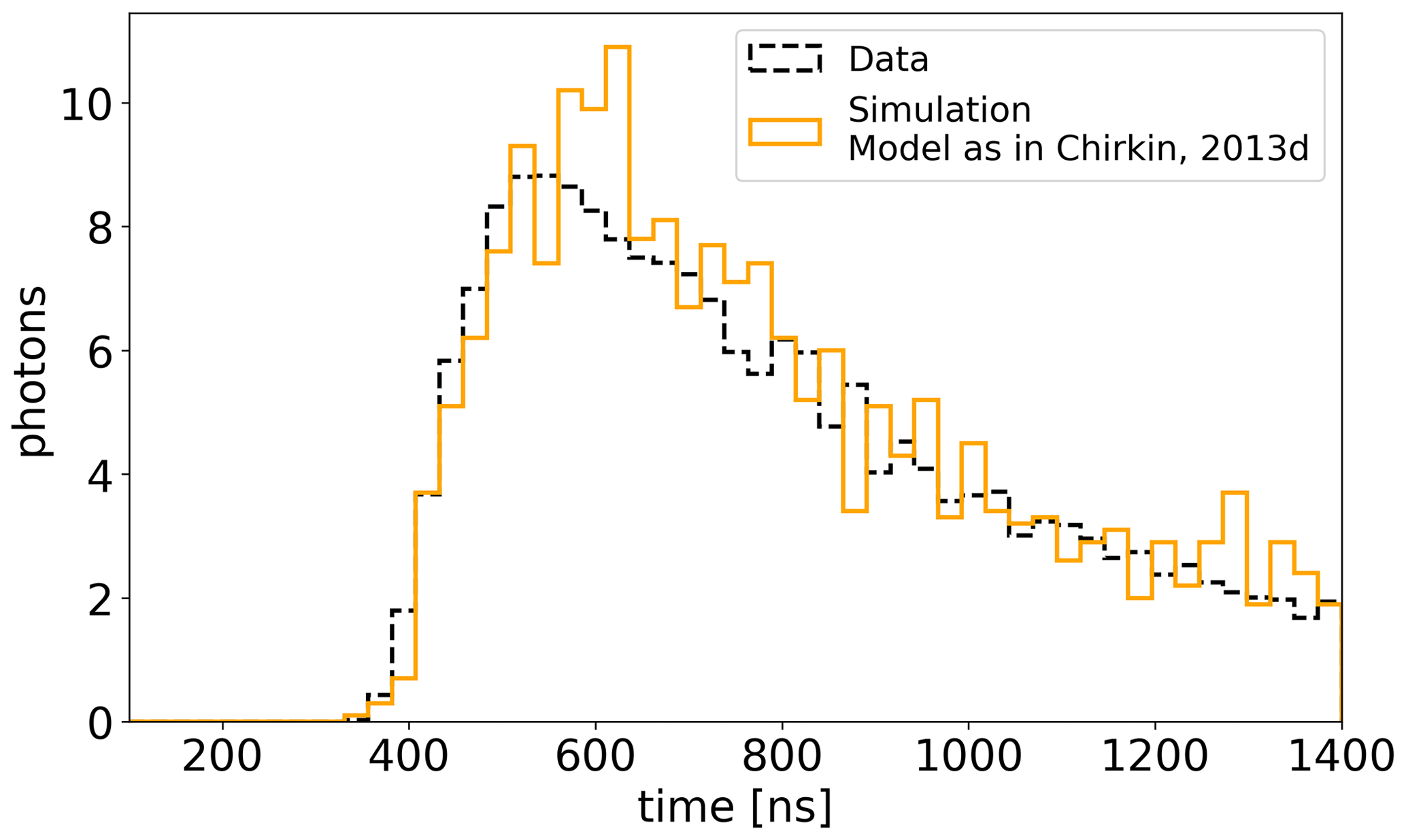
Figure 2 Example flasher light curve in 25 ns binning. DOM 50 on string 1 emits light which is detected by DOM 55 on string 8 about 150 m away. The data are averaged over 240 repetitions. The simulation is averaged over 10 repetitions.

The per-event average expectation in each bin is a function of the sampled ice properties and nuisance parameters, such as a per-LED light yield, a timing offset of the light emission with regard to the LED trigger, and the absolute LED orientations. The likelihood function used for comparing this expectation to data is given by

$$\begin{array}{}\text{(3)}& -\ln \mathcal{L}=\sum _i\left[s_i\ln {\displaystyle \frac{s_i/n_{\mathrm{s}}}{{\mathit{\mu }}_{\mathrm{s}}^i}}+d_i\ln {\displaystyle \frac{d_i/n_{\mathrm{d}}}{{\mathit{\mu }}_{\mathrm{d}}^i}}+{\displaystyle \frac{\mathrm{1}}{\mathrm{2}{\mathit{\sigma }}^{\mathrm{2}}}}{\left(\ln {\displaystyle \frac{{\mathit{\mu }}_{\mathrm{d}}^i}{{\mathit{\mu }}_{\mathrm{s}}^i}}\right)}^{\mathrm{2}}\right],\end{array}$$

where i denotes a receiver DOM and time bin of its light curve, s_i and d_i the photon count in simulation and data for this bin, respectively, n_s and n_d the simulation repetitions and number of data events, σ the model error, and μ_s and μ_d the simulation and data expectation values; −ln ℒ is abbreviated as LLH in the following.

The model error takes into account potential discrepancies in reproducing data with a simulation that may be incomplete or may use nonideal parameterizations. Using the model error, it is assumed that a difference between the expectation values of simulations and data can exist even at the best-fit point, ${\mathit{\mu }}_{\mathrm{s}}\ne {\mathit{\mu }}_{\mathrm{d}}\ne (s_i+d_i)/(n_{\mathrm{s}}+n_{\mathrm{d}})$. This is modeled through the penalty term in the likelihood (Chirkin, 2013b). This extension also requires an optimization of the now in principle independent expectation values within the likelihood calculation and is performed as described by Chirkin (2013b).

This likelihood (Chirkin, 2013b) improves on a common Poisson likelihood by taking into account the uncertainty of the expectation caused by the small statistics of the simulated data compared to the experimental data. Therefore, the expectation is optimized including the knowledge of the limited statistics of both the simulated and experimental data. In the limit of infinite statistics of simulated data this likelihood converges to a saturated Poisson likelihood.

The parameters of the ice model are generally obtained through likelihood scans, where each scan point is one realization of the ice model parameters tested against flasher data. The timing offset and LED intensity nuisance parameters are optimized for each realization analytically and through a number of low statistics iterations.

The likelihood method described above does not, in general, fulfill Wilks' theorem (Wilks, 1938), which would, under certain conditions, allow one to approximate the distribution of the likelihood ratio between the best-fit and null hypotheses with a chi-squared distribution. As such, the log-likelihood contour of a one-dimensional likelihood scan enclosing the minimum by ΔLLH of 1 does not represent a 1σ statistical uncertainty. Instead, the spread in LLH values equivalent to the 1σ uncertainty is obtained by re-simulating a realization close to the optimum a number of times and computing the standard deviation of the resulting LLH values.

Fitting the flasher data, the statistical errors in the ice properties, in particular the layered absorption and scattering coefficients, are entirely due to the limited simulation statistics but generally remain below 1 %. Thus the statistical error is subdominant compared to systematic biases introduced through incomplete modeling. This bias is hard to quantify, in particular due to the enormous computational cost. Taking into account the limited knowledge of the relative detection efficiencies of the DOMs, the discrepancy between fitted values using only horizontal or only tilted LEDs and different realizations of the modeled scattering function, the systematic uncertainty on the scale of absorption and scattering coefficients is estimated to be around 5 %.

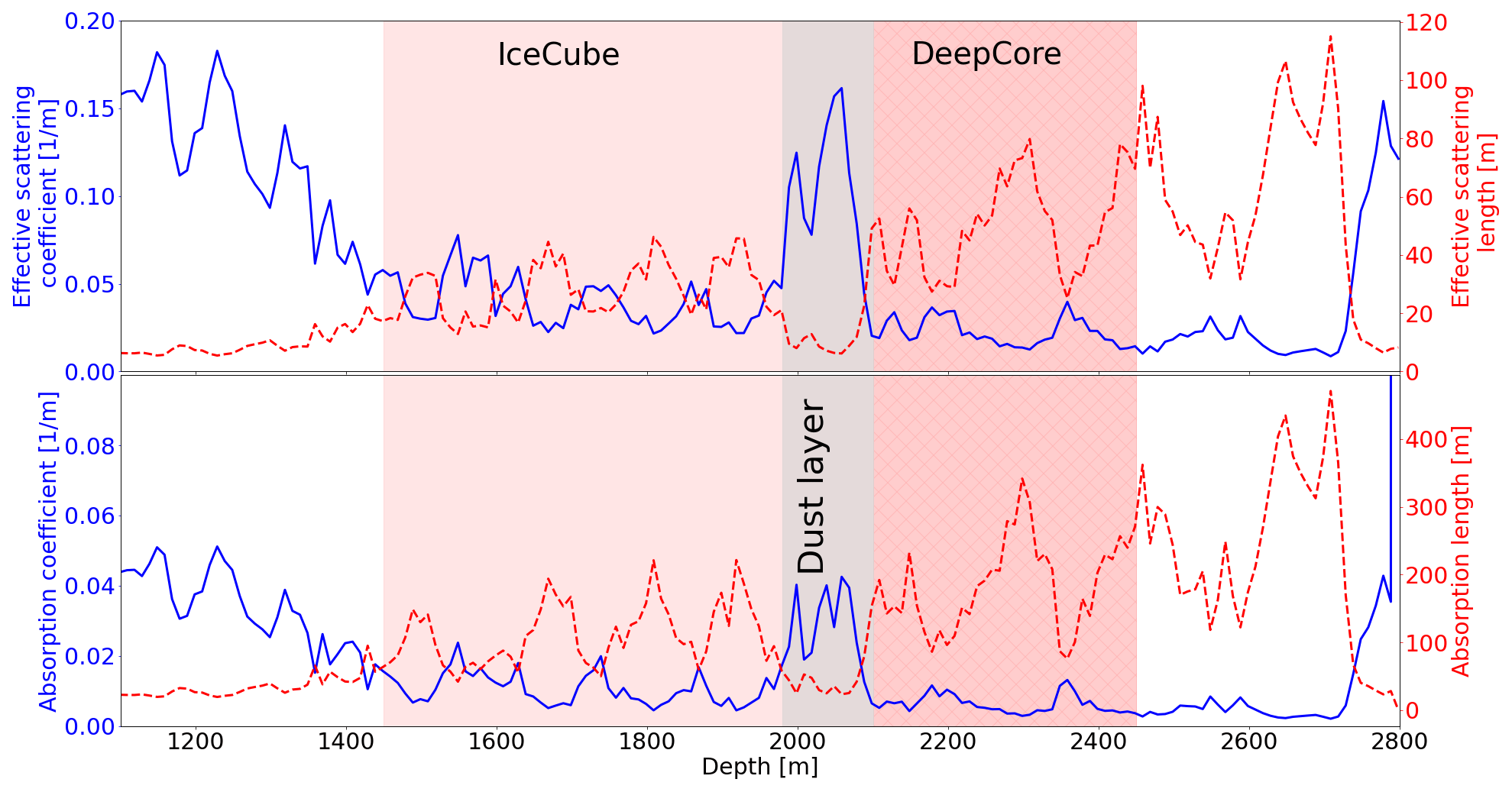
Figure 3 Stratigraphy of fitted absorption and scattering strength. Properties above the detector (<1450 m) are taken from AMANDA measurements (Ackermann et al., 2006) or are extrapolated from dust logger data. Properties below (>2450 m) are extrapolated using the stratigraphy as obtained from the EDML ice core (Bay et al., 2010) and ice age vs. depth curve from Price et al. (2000).

3.4 The South Pole Ice Model (SPICE)

Employing the experimental and analysis methods described above, absolute absorption and scattering coefficients and their wavelength scaling have been measured for all instrumented depths as described in detail by Ackermann et al. (2006) and Aartsen et al. (2013c). The resulting model, called the South Pole Ice Model (SPICE), continues to be updated and refined as new aspects of the instrumentation such as the properties of the refrozen drill columns (Chirkin et al., 2021) as well as previously unconsidered features in the ice begin to be modeled. The stratigraphy, used as the starting point for this study, is shown in Fig. 3. At the instrumented depths, absorption lengths mostly exceed 100 m, with the most significant exception being a region at around 2000 m, in IceCube commonly referred to as “the dust layer”. This has been associated with a period of continuously elevated dust concentrations during a stadial around 65 000 years ago (Ackermann et al., 2006).

While primarily developed and employed for the simulation of particle interactions, the deduced model parameters are also informative of ice properties in general. Most prominently the lowest measured absorption coefficients now serve as a reference for an upper limit on ice-intrinsic absorption as compiled by Warren and Brandt (2008). The technique of time-resolved photon counting has recently also been adopted by Allgaier et al. (2022) to deduce impurity concentrations in firn.

3.4.1 Layer undulation

One relevant complication is the undulations of layers of equal optical properties within the instrumented volume. As established from ground-penetrating radar sounding (e.g., Fujita et al., 1999) ice isochrons can be traced over thousands of kilometers. While the ice surface is generally flat, deeper layers tend to gradually follow the topography of the underlying bedrock, with additional features such as upwarping and folds in basal ice (e.g., Cooper et al., 2019; Dow et al., 2018; MacGregor et al., 2015).

Available radar data generally do not have the spatial resolution required to map features within the instrumented volume of IceCube. Instead the depth offset of characteristic features as observed in the dust logger data from seven different IceCube holes has been used to interpolate the depth-dependent layer undulations assuming an undisturbed chronological layering as described by Aartsen et al. (2013a). Layers with roughly constant scattering and absorption change in depth by as much as 60 m as one moves across the ∼1 km detector. This gradient is mainly found along the SW direction, orthogonal to the flow direction. At the location of IceCube, the ice flows in the direction grid NW at a rate of about 10 m yr⁻¹ (Lilien et al., 2018), slowly draining into the Weddell Sea after flowing through the Pensacola–Pole Basin (Paxman et al., 2019).

Within the context of the ice model, the depth offset at which a given ice layer is encountered relative to the stratigraphy as defined in the center of the detector is generally referred to as “tilt”. The orientation of the main gradient is termed “tilt direction”. Within the context of this work the tilt model as described by Aartsen et al. (2013c) is employed.

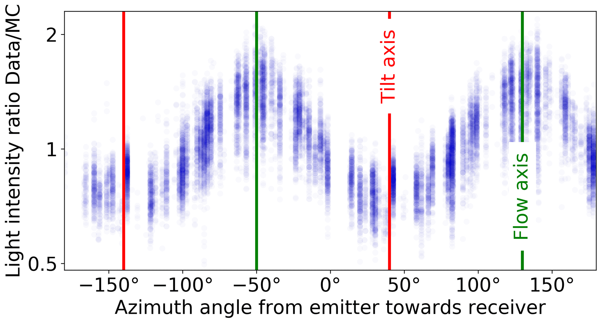
Figure 4 Ice optical anisotropy seen as azimuth-dependent intensity excess in flasher data. Each dot is the observed intensity ratio for one pair of light-emitting and light-detecting DOMs comparing data to a simulation with no anisotropy modeling enabled. The tilt and flow directions are shown for reference.

4 The ice optical anisotropy

4.1 Experimental signature

Given the optical modeling discussed so far, the amount of light received from an isotropic source should not depend on the direction of the receiver with respect to the emitter. However, if we consider many DOMs, each with their 12 calibration LEDs and at a random azimuthal orientations in the refrozen drill holes, as isotropic emitters and we average observations along different directions of emitter–receiver pairs of DOMs, we find a significant directional dependence. About twice as much light is observed along the direction of the ice flow compared to the orthogonal ice tilt direction when measured at distances of ∼125 m, as seen in Fig. 4. This ice optical anisotropy was first discussed in 2013 (Chirkin, 2013d). The experimental arrival time distributions are nearly unchanged compared to a simulation expectation without anisotropy (as will be evident in Fig. 6).

4.2 The anisotropy axis

A determination of the axis of the ice optical anisotropy can be achieved independent of any model assumption by fitting the phase of the sinusoidal intensity modulation as shown in Fig. 4. To obtain spatial resolution, the data are binned in emitting DOMs, either within a tilt-corrected depth range or by string number. Thus the data are dominated by propagation in a given depth range or in the vicinity of a given string. Figure 5 shows the resulting anisotropy axes.

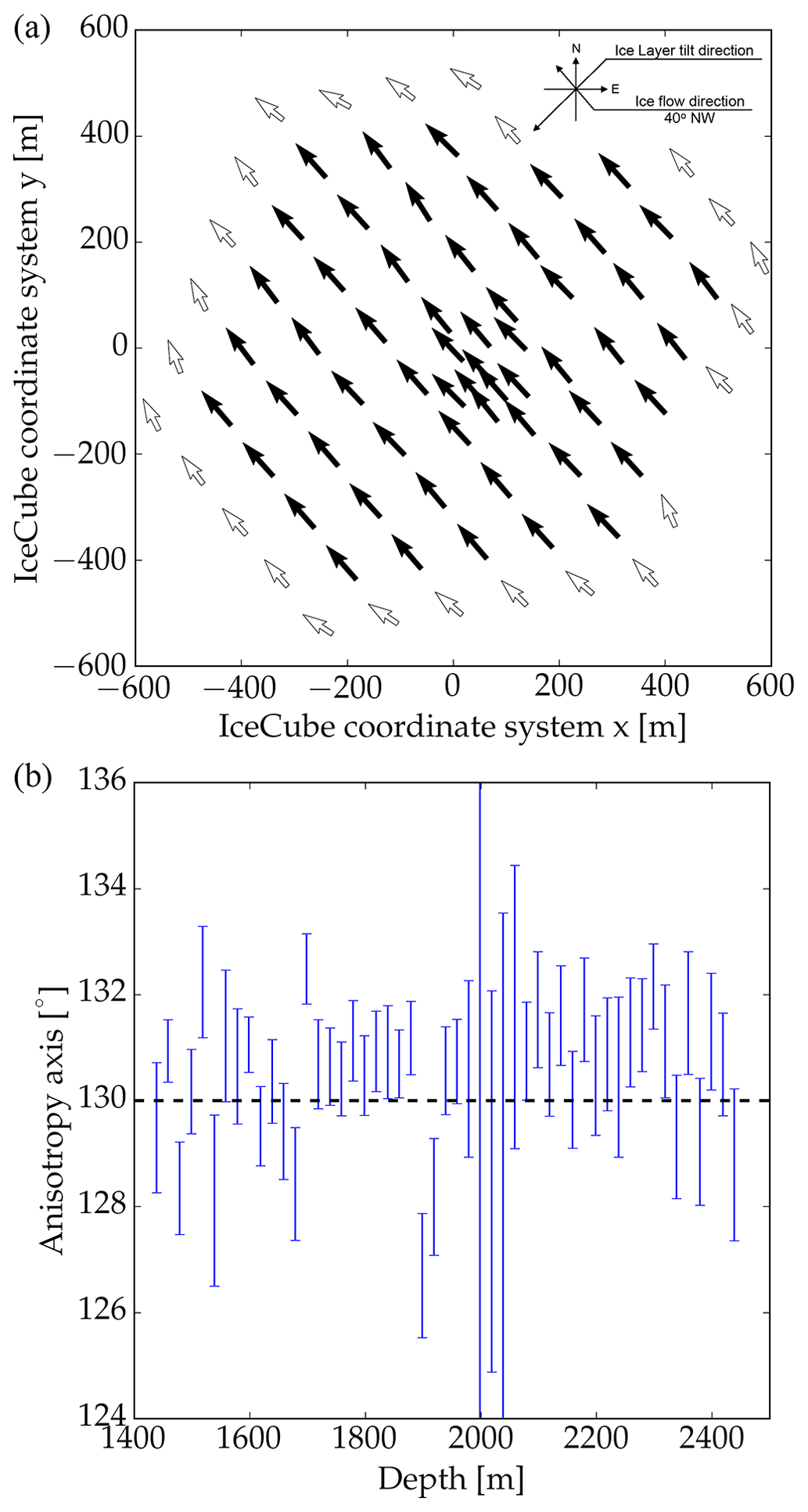
Figure 5 Measured anisotropy axes as a function of lateral position averaging over all depth (a) and as a function of depth averaging over all strings (b). Strings on the perimeter of the detector have been excluded, as the lack of symmetric neighbors leads to potentially biased results. The sensitivity is greatly reduced in the region of strongest scattering around 2000 m. The dashed line indicates the anisotropy angle averaged over all strings.

The anisotropy axis is seen to have constant direction throughout the entire detector and is considered constant for all following investigations. The resolution is around 1^∘ everywhere, except in the strongly scattering and absorbing dust layer. Edge strings are also disregarded as the lack of symmetric neighbors potentially leads to biased results.

The absolute direction is 130^∘ in the IceCube coordinate system (an azimuth of 0^∘ is defined with respect to the positive x axis in Fig. 5 and runs counterclockwise), equivalent to the 40^∘ W meridian in the universal polar stereographic coordinate system, and is in excellent agreement with present-day flow direction as measured using a GPS stake field by Lilien et al. (2018).

As a part of the models described in Sects. 4 and 5 a possible elevation angle to the anisotropy axis has been considered. In both cases a near-constant elevation angle of 5^∘ on average has been fitted. However, this fit is difficult to completely disentangle from effects that may arise as a result of mis-modeling of the layer undulations or the optical properties of the refrozen drill holes (Chirkin et al., 2021). As the resulting improvement in data–simulation agreement was seen to be small, this additional complication is not further considered here. As will be explained later, this elevation angle would directly relate to an elevation angle of the crystal orientation fabric.

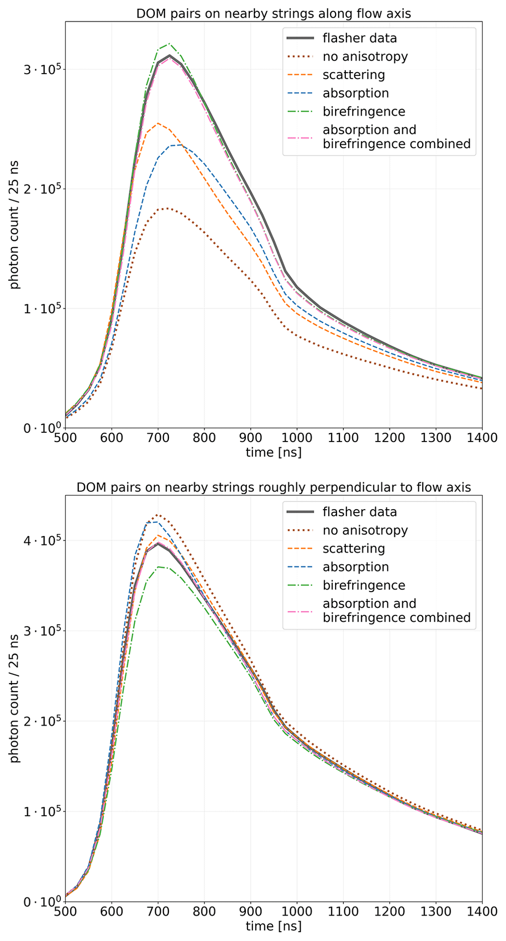
Figure 6 Comparison of fit quality achieved with different models for the ice optical anisotropy. Shown are photon arrival time distributions (summed counts in 25 ns time bins) for all nearest-pair emitters and receivers, roughly aligned along and perpendicular to the ice flow. As more emitter–receiver pairs are included in the perpendicular case compared to the case along the ice flow, the total photon counts are not directly comparable between the two plots and should instead be compared to the curve titled “flasher data” within each plot. While the array geometry is well aligned with the flow axis, the nearest inter-module propagation direction perpendicular to the flow is roughly 30^∘ off. The “absorption” and “scattering” models represent ad hoc, directional modifications to Mie scattering and absorption but are unable to describe timing and intensity simultaneously. “Birefringence” refers to the microstructure-based effect introduced in this paper. A combination of the absorption and birefringence model yields the closest match to data to date.

4.3 Early empirical modeling

Following the paradigm that ice optical properties are driven by Mie scattering on impurities, early attempts tried to model the anisotropy through directional modifications of absorption and scattering. In the original parameterization presented by Chirkin (2013d), it was argued that due to time and space reversal symmetries the absorption length and geometric scattering length cannot be direction-dependent. Therefore the anisotropy was implemented as a modification to the scattering function, the only remaining Mie scattering parameter. This effectively results in a change in the effective scattering coefficient as a function of the propagation direction. Photons propagating along the flow axis experience less scattering than photons propagating along the tilt axis or inclined from the horizontal.

While not derived from first-principles Mie calculations, the parameterization was justified to be a plausible result of elongated impurities becoming preferentially aligned by the flow and thus introducing a direction dependence to the scattering function. While several glaciological studies (Potenza et al., 2016; Simonsen et al., 2018; Gebhart, 1991) explore the shapes of impurities, elongations for different impurities are not well established, nor is there to our knowledge any evidence of elongated impurities becoming oriented with the flow. Alternatively a directionality of Mie scattering may be believed to be the result of inhomogeneous impurity distributions, with some impurity types known to preferentially aggregate on the grain boundaries (Stoll et al., 2021b; Durand et al., 2006). Yet the derivation of Mie scattering properties only depends on the volumetric particle densities and is independent of homogeneity. In the context of studying the ice optical anisotropy, Rongen (2019) explicitly tested this in a number of simulated toy experiments and verified that inhomogeneous impurity distributions cannot lead to large-scale anisotropy.

An evaluation of the data–simulation agreement is shown in Fig. 6. It shows summed photon arrival time distributions for all nearest emitter–receiver pairs, roughly aligned along and perpendicular to the ice flow for a variety of anisotropy models and the employed flasher data. The scattering-based anisotropy model results in more intensity being observed along the flow axis. However, substantial disagreement remains between the model and the observed data. As scattering is reduced in the flow direction light arrives earlier on average. The resulting change in the rising edge position is strongly penalized in the fit and limits the amount of intensity that can be recovered.

To reduce the shift of the rising edge, a directional modification to Mie absorption was considered as an alternative by Rongen (2019). A factor of 11 modulation of the absorption coefficient was required to fit the data, which seems unphysical. As evident from Fig. 6, this model results in a delayed rising edge for propagation along the flow direction as desired and did result in an improved data description compared to the scattering-based model described earlier, but it is also unable to fully match the intensity difference to data.

To conclude, while resulting in partially successful effective descriptions, directional modifications to Mie scattering or absorption cannot reproduce observations nor are such modifications well motivated on first principles.

5 Light diffusion in birefringent polycrystals

5.1 The electromagnetics of uniaxial, birefringent crystals

Departing from the paradigm that optical properties are purely driven by impurities, let us consider the impact of the microstructure of the ice itself on light propagation.

Light diffusion in birefringent, polycrystalline materials was discussed as early as 1955 by Raman and Viswanathan (1955). While the literature agrees that the combined effect of ray splitting on many crystal interfaces will lead to a continuous beam diffusion, the resulting diffusion patterns remained largely unexplored. Price and Bergström (1997) already considered this average overall diffusion in the context of Cherenkov neutrino telescopes but disregarded it as subdominant compared to scattering on impurities.

In a homogeneous, transparent, and non-magnetic medium the relation between the electric field and the displacement field as well as the magnetic fields is given as (Landau and Lifshitz, 1960)

$$\begin{array}{}\text{(4)}& \mathit{B}=\mathit{H},\mathit{D}=\mathit{ϵ}\mathit{E}.\end{array}$$

As the dielectric tensor ϵ is symmetric, one can always find a coordinate system where it is diagonal $\mathit{ϵ}=\text{diag}(n_x^{\mathrm{2}},n_y^{\mathrm{2}},n_z^{\mathrm{2}})$, with n_i being the refractive index along the given axis. Uniaxial crystals, such as ice in glacial environments, have two distinct refractive indices: $n_x=n_y\equiv n_{\mathrm{o}}\ne n_z\equiv n_e$. The axis of the refractive index n_e defines the optical axis and coincides with the c axis.

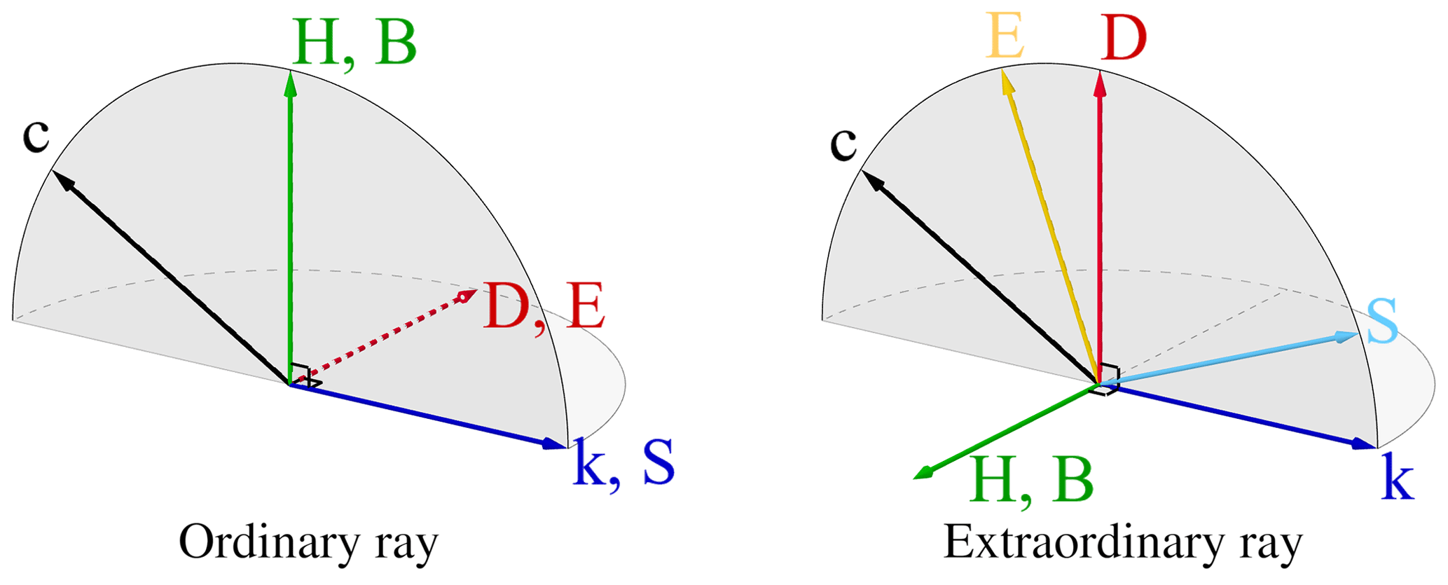
Figure 7 Orientation of all electromagnetic vectors for the ordinary and extraordinary ray with respect to the crystal axis (c axis). See text for a detailed explanation of this figure.

A light ray entering a uniaxial crystal is split into an ordinary wave and an extraordinary wave of orthogonal polarizations. Figure 7 visualizes the orientations of all electromagnetic vectors, the plane spanned by the optical axis c, and the wave vector k is highlighted in gray. The electric field vector E and the displacement vector D for the ordinary wave are always co-linear with each other and perpendicular to both the optical axis of the crystal and the parallel propagation vectors k and S. However, the electric field E for the extraordinary wave is not, in general, perpendicular to the propagation vector k. It lies in the plane formed by the propagation vector and the displacement vector. The electric field vectors of these waves are mutually orthogonal (Zhang and Caulfield, 1996). The energy flow is given by the Poynting vector $\mathit{S}=\frac{c}{\mathrm{4}\mathit{\pi }}\mathit{E}\times \mathit{H}$. For the extraordinary wave, the Poynting vector S is not parallel to k.

While the ordinary ray always propagates with the ordinary refractive index n_o, the refractive index of the extraordinary ray depends on the opening angle θ between the optical axis and the wave vector k (as described in a later section with Eq. 7). The difference to n_o is largest when the optical axis and the wave vector are perpendicular. In this case the extraordinary ray propagates with the refractive index n_e.

Table 1 Refractive indices of ice taken from Petrenko and Whitworth (2002).

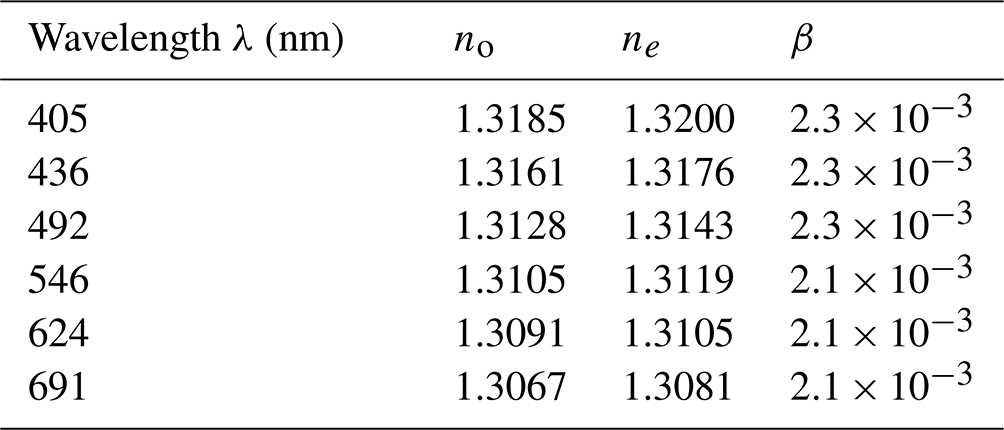
The birefringence strength can be expressed as

$$\begin{array}{}\text{(5)}& \mathit{\beta }={\left({\displaystyle \frac{n_e}{n_{\mathrm{o}}}}\right)}^{\mathrm{2}}-\mathrm{1}.\end{array}$$

For ice β is $\approx \mathrm{2}\times {\mathrm{10}}^{-\mathrm{3}}$ across the entire visible wavelength spectrum. Refractive indices at specific wavelengths can be found in Table 1 (Petrenko and Whitworth, 2002).

5.2 Analytic calculation of a single grain boundary transition

Assuming an arbitrary ray incident on a plane interface, we first calculate the four possible wave vectors, the ordinary and extraordinary refracted rays, and the ordinary and extraordinary reflected rays. Given the wave vectors, the four associated Poynting vectors are calculated from the boundary conditions, yielding the energy flow and as such probable photon directions.

5.2.1 Wave vectors

Figure 8 shows the situation at hand: an incoming wave vector k intersects the interface and is split into four outgoing wave vectors r. The coordinate system can always be chosen such that the surface normal n is along the y axis and that the surface components of k, and as such r, are along the x axis. Here we implicitly assume, as an approximation, that the boundary surface is a perfect plane infinite in its extension and, without a loss of generality, that the incoming and outgoing waves are all plane waves.

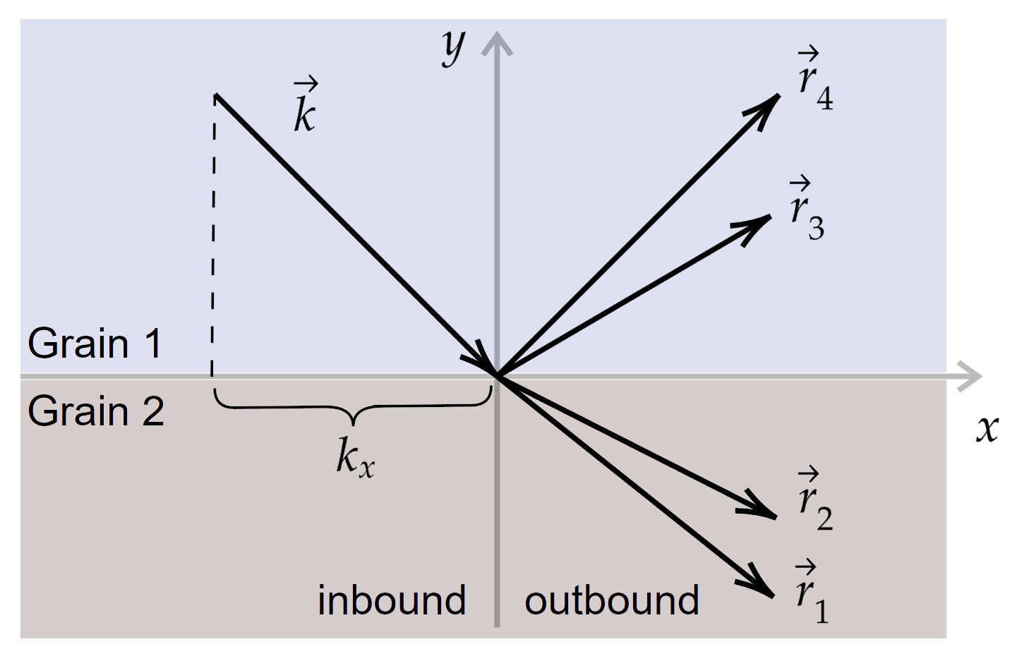
Figure 8 Sketch of wave vectors for the incident, reflected, and refracted rays. The surface component is identical for all rays.

Because of translational symmetry of the interface surface, the surface components of all wave vectors are identical (Landau and Lifshitz, 1960): k_x=r_x. As the wave number is given by $k=\frac{\mathrm{2}\mathit{\pi }}{\mathit{\lambda }}$, we can define a vector n such that $\mathit{k}=\mathit{\omega }\mathit{n}/c$, whose magnitude n is the direction-dependent refractive index $n=\sqrt{\mathit{ϵ}\left(\mathit{\theta }\right)}$. As such the magnitude of the wave vector is proportional to the refractive index and we shall simplify $\left|\mathit{k}\right|=n$ in the following.

Outgoing ordinary rays

Given the magnitude n_o and surface component k_x of the wave vector the y component is

$$\begin{array}{}\text{(6)}& r_y=\pm \sqrt{n_{\mathrm{o}}^{\mathrm{2}}-k_x^{\mathrm{2}}}.\end{array}$$

The outgoing ordinary ray of an inbound ordinary ray is not deflected, as it does not see a change in refractive index. In the case of no birefringence, one obtains Snell's law for refraction and the usual law for reflection ($r_y=-k_y$).

Outgoing extraordinary ray

Determining r_y for the extraordinary rays follows the same logic, only with a refractive index which depends on the opening angle θ between the outgoing wave vector $\mathit{r}=(r_x,r_y)$ and the optical axis $\mathit{a}=(a_x,a_y,a_z)$:

$$\begin{array}{}\text{(7)}& {\displaystyle \frac{\mathrm{1}}{n^{\mathrm{2}}}}={\displaystyle \frac{\mathrm{1}}{n_e^{\mathrm{2}}}}+\left({\displaystyle \frac{\mathrm{1}}{n_{\mathrm{0}}^{\mathrm{2}}}}-{\displaystyle \frac{\mathrm{1}}{n_e^{\mathrm{2}}}}\right)\cdot {\cos }^{\mathrm{2}}\mathit{\theta }.\end{array}$$

The optical axis is given by the optical axis of medium 1 for the reflected ray and of medium 2 for the refracted ray. Rewriting cos (θ) as scalar product between the wave vector and the optical axis gives

$$\begin{array}{}\text{(8)}& {\displaystyle \frac{\mathrm{1}}{n_e^{\mathrm{2}}}}+\left({\displaystyle \frac{\mathrm{1}}{n_{\mathrm{o}}^{\mathrm{2}}}}-{\displaystyle \frac{\mathrm{1}}{n_e^{\mathrm{2}}}}\right)\cdot {\displaystyle \frac{(a_x{r}_x+a_y{r}_y{)}^{\mathrm{2}}}{n^{\mathrm{2}}}}-{\displaystyle \frac{\mathrm{1}}{n^{\mathrm{2}}}}=\mathrm{0}.\end{array}$$

Here $n^{\mathrm{2}}={\mathit{r}}^{\mathrm{2}}=r_x^{\mathrm{2}}+r_y^{\mathrm{2}}$. The solution is

$$\begin{array}{}\text{(9)}& r_y={\displaystyle \frac{-\mathit{\beta }{a}_x{a}_y{r}_x\pm \sqrt{D}}{\mathrm{1}+\mathit{\beta }{a}_y^{\mathrm{2}}}},\end{array}$$

with

$$\begin{array}{}\text{(10)}& {\displaystyle }D& {\displaystyle }=(\mathit{\beta }{a}_x{a}_y{r}_x{)}^{\mathrm{2}}-(\mathrm{1}+\mathit{\beta }{a}_y^{\mathrm{2}}\left)\right(r_x^{\mathrm{2}}\cdot (\mathrm{1}+\mathit{\beta }{a}_x^{\mathrm{2}})-n_e^{\mathrm{2}})\text{(11)}& {\displaystyle }& {\displaystyle }=n_e^{\mathrm{2}}\cdot (\mathrm{1}+\mathit{\beta }{a}_y^{\mathrm{2}})-r_x^{\mathrm{2}}\cdot (\mathrm{1}+\mathit{\beta }\cdot (a_x^{\mathrm{2}}+a_y^{\mathrm{2}}\left)\right).\end{array}$$

Of the two solutions the direction appropriate for the reflected or refracted ray is chosen and the other discarded. In the case of no birefringence (β=0) we again obtain the solution for the ordinary ray.

5.2.2 Poynting vectors

Once the wave vector directions are determined, the boundary continuity conditions can be written for normal components of D and B and for tangential components of E and H. If n is a normal vector perpendicular to the interface surface, we have

$$\begin{array}{}\text{(12)}& {\displaystyle }& {\displaystyle }\mathit{n}\cdot {\mathit{D}}_{\mathbf{1}}=\mathit{n}\cdot {\mathit{D}}_{\mathbf{2}},\mathit{n}\cdot {\mathit{B}}_{\mathbf{1}}=\mathit{n}\cdot {\mathit{B}}_{\mathbf{2}},\text{(13)}& {\displaystyle }& {\displaystyle }\mathit{n}\times {\mathit{E}}_{\mathbf{1}}=\mathit{n}\times {\mathit{E}}_{\mathbf{2}},\mathit{n}\times {\mathit{H}}_{\mathbf{1}}=\mathit{n}\times {\mathit{H}}_{\mathbf{2}}.\end{array}$$

Here the subscript 1 indicates the total sum of fields for incident and reflected waves, and the subscript 2 indicates the fields of the refracted waves propagating away from the boundary surface in the second medium. Since B=H two of the equations above simply imply that B₁=B₂ and H₁=H₂. Together with the boundary conditions for D and E, this is a system of six linear equations. These equations are sufficient to determine the amplitudes of four outgoing waves: two reflected (ordinary and extraordinary) and two refracted (also ordinary and extraordinary). Since we only have four unknowns, two of these equations are necessarily co-linear with the rest if the wave vectors were determined correctly.

From the solution to the linear equation system the Poynting vectors and as such the photon directions of the (up to) four outgoing rays are calculated. The relative intensity of these rays, as usually denoted in Fresnel coefficients, is derived from the Poynting theorem, which for our case (no moving charges, no temporal change in total energy) is given as

$$\begin{array}{}\text{(14)}& \underset{\partial V}{∯}\mathit{S}\cdot \mathrm{d}\mathit{A}=\mathrm{0},\end{array}$$

where ∂V is the boundary of a volume V surrounding the interface. The choice of volume is arbitrary. A simple choice is a box around the interface. In the limit of an infinitely thin but wide box, it is evident that the sum of Poynting vector components normal to the interface plane is conserved.

Evanescent waves, i.e., waves with a complex wave vector, which decay away from the boundary surface and arise when the discriminant in the wave vector equation (Eq. 10) is negative, will necessarily yield vanishing contributions to such a sum. As the photon interacts with a boundary there is a brief flow of energy along the surface boundary within evanescent solutions (if any), but no energy flows away from the boundary within such solutions. The evanescent waves need to be considered when solving the boundary conditions as given in Eq. (13).

After deriving the solution presented here, we learned of the paper by Zhang and Caulfield (1996) and found that our approach is similar to the one they described.

5.3 Simulating diffusion patterns

Based on the calculations above, a photon propagation simulation for birefringent polycrystals was implemented in C++. At each grain transition, the outgoing photon is then chosen randomly, with probabilities proportional to the (up to) four normal components of the non-evanescent Poynting vectors to account for the relative intensities.

The resulting diffusion patterns, defined as the distribution of photon directions after crossing a given number of grains, depend on two factors related to the polycrystal configuration.

The assumed probability density distribution of c-axis orientations, which is the crystal orientation fabric, determines the refractive indices a photon will encounter. As measured c-axis distributions offer limited statistics and are restricted to the encountered fabric states, it is necessary here to statistically sample generic c-axis distributions. Appendix A briefly summarizes the different kinds of fabric and describes the approach developed to sample an arbitrary number of c axes based on Woodcock parameters $\log (S_{\mathrm{1}}/S_{\mathrm{2}})$ and $\log (S_{\mathrm{2}}/S_{\mathrm{3}})$, the usually published statistical moments associated with the fabric orientation tensor. Woodcock parameters for the ice at the South Pole are available from the South Pole Ice Core SPC14 (Casey et al., 2014), drilled by the SPICEcore project in 2014–2016 at a location ∼1 km from the IceCube array using the Intermediate Depth Drill designed and deployed by the U.S. Ice Drilling Program (IDP) (Johnson et al., 2014)).

It reached a final depth of 1751 m (Winski et al., 2019), which corresponds to a depth of ∼1820 m in the IceCube ice model (see Fig. 3), accounting for the layer undulation between the two reference points. The c-axis distributions have been measured by Voigt (2017) at all depths and show an exceptionally clean girdle fabric at the overlapping depth as summarized in Fig. A1.

As evident from Snell's law, in addition to the change in refractive index, the slope of the interface surface also dictates the refraction angle at a grain boundary transition. Thus the distribution of grain boundary plane orientations, resulting from a given grain shape, needs to be modeled in addition to the crystal orientation fabric. Appendix B shows that the surface orientation density of an ensemble of ice crystals, simulated as a polyhedral tessellation of a volume, can be approximated using a triaxial ellipsoid that represents the average shape. For a generalized ellipsoid the diffusion patterns are thus not only a function of the opening angle between the initial photon direction and the flow (as expected from the crystal orientation fabric), but also depend on the absolute zenith and azimuth orientation of the propagation direction with respect to the flow. Employing an alternative parameterization, developed prior to the one introduced in Sect. 6.1, it was determined early on that fully triaxial ellipsoids offer no advantage to describing the flasher data compared to prolate spheroids, where the major axis is aligned with the flow and the horizontal and vertical minor axes are identical. These spheroids, described by the size of the major axis and an elongation, are what we restrict ourselves to here. Grain size and shape distributions have not yet been fully published by the SPICEcore collaboration but are expected from preliminary material shown at conferences (Alley et al., 2021) as well as other cores (e.g., Weikusat et al., 2017; Lipenkov et al., 1989; Stoll et al., 2021a; Faria et al., 2014a) to be on the millimeter scale with elongations of at most a factor of 2. Both fabric and grain shape are not directly taken from ice core data but are determined from the flasher data (see Sect. 6.3).

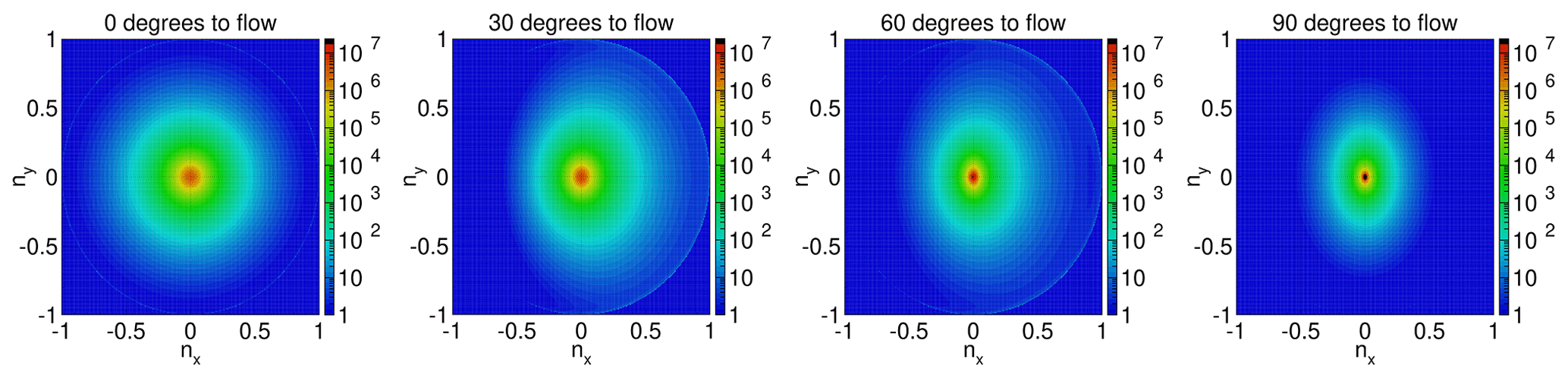
Figure 9 Example diffusion patterns after photon propagation through 1000 crystals (roughly equivalent to 1 m) with a perfect girdle distribution of c-axis orientations. The initial directions of the emitted photon point perpendicularly out of the picture, with an opening angle to the flow as indicated. The figures histogram the final direction vectors of 10⁸ photons each. The change in diffusion (width of the distributions) as well as the subtle effect of photon scattering towards the ice flow (towards the right) can be seen.

Simulated diffusion patterns after crossing 1000 grain boundaries for four initial propagation directions relative to the flow axis and assuming on average spherical grains as well as a perfect girdle fabric are shown in Fig. 9. The overall diffusion is largest when propagating along the flow direction and becomes continuously smaller towards the tilt direction. For intermediate angles the distribution is slightly asymmetric, resulting in a mean deflection towards the ice flow axis. The diffusion being largest along the flow axis results in a reduction of intensity in this direction, which is contrary to observations. The deflection, however, slowly diverts intensity from the tilt direction and overpopulates the flow (see Fig. 10) direction. Thus a good fit to the data should be obtainable by finding the right combination of crystal orientation fabric, shape, and crystal size as it changes the number of crystals per distance (see Sect. 6.1).

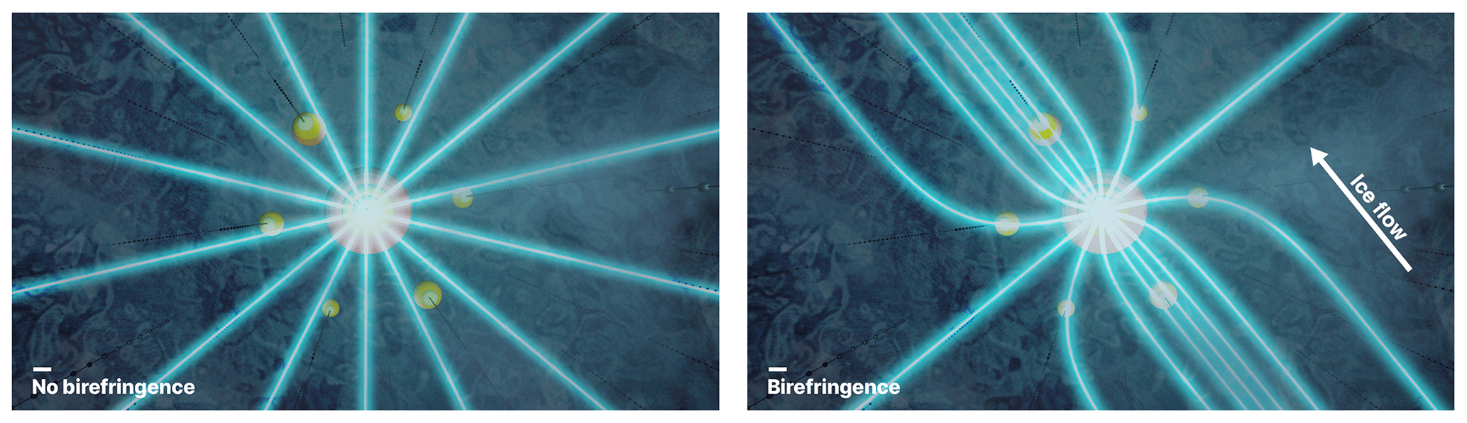
Figure 10 Artist illustration visualizing the deflection concept. Without birefringence light streams out radially from an isotropic light source. With birefringence rays get slowly deflected towards the flow axis. The effects of scattering and diffusion are not shown. The hexagonal pattern of the IceCube array around the light source is shown.

To validate our calculations and implementation, a polycrystal was realized in Zemax, a commercial optics simulation program, using a polycrystal tessellation simulated using Neper: Polycrystal Generation and Meshing (Quey et al., 2011) and exporting each interlocking monocrystal as a CAD object. The same quantitative behavior as described above is reproduced. This approach, however, does not allow for a flexible configuration and is slow to simulate reasonable photon statistics.

5.4 Comparison to fabric-induced anisotropies in radar measurements

Before incorporating the diffusion patterns into the overall IceCube simulation and fitting new ice parameters, we will discuss some conceptual differences of the birefringence-induced optical anisotropy in comparison to birefringence effects in radar measurements, which many readers may be more familiar with.

When probing the ice with radio waves the employed wavelength is orders of magnitude larger than the crystal size. Thus the waves do not interact with individual grains, and propagation is only influenced by the bulk dielectric tensor, weighting the per-crystal dielectric tensor with their relative occurrence. Since the birefringence strength $\mathit{\beta }=(n_e/n_{\mathrm{o}}{)}^{\mathrm{2}}-\mathrm{1}$ is an order of magnitude larger in radio (β∼1 %) compared to optical waves (β∼0.2 %), the available observables are primarily direction-dependent timing delays (either of the entire pulse or measured as a phase difference) and – for polarimetric systems – changes in the received polarization with respect to the emitted polarization.

Given the timing precision of IceCube and given the low birefringence strength in the optical regime, the effect of birefringence on timing will not be relevant here. Even assuming the unrealistic case in which one ray propagates purely with the ordinary and another with the extraordinary refractive index, the propagation delay over 250 m would only amount to ∼1 ns, which is undetectable with IceCube. Polarization is also not an available observable using IceCube data. Since each crystal effectively acts as a polarization analyzer and a large number of these are randomly sequenced, the diffusion patterns also do not depend on the initial polarization.

Instead, since the wavelength is small compared to the crystal size, light rays experience the individual grains as distinct objects and slowly diffuse through the continued refractions and reflections at the grain boundaries. Given a mean elongation or equivalently a preferential c-axis distribution in addition to the diffusion, rays get on average slowly deflected towards the elongation axis. To our knowledge this is a newly discovered optical effect not described in the literature before.

6 The birefringence ice model

6.1 Parameterizing diffusion patterns

While the simulation described above in principle scales to arbitrary crystal counts, it is computationally unfeasible to explicitly simulate every single grain boundary with every simulated photon traveling dozens to hundreds of meters. For this reason, an analytic parameterization was developed, which allows describing the cumulative effect at large scales.

Diffusion patterns have been simulated for a wide range of spheroid elongations (1–3) and fabric parameters (spanning the plane of Woodcock parameters between 0.1 and 4 in both dimensions). As evident from the example in Fig. 9, these diffusion patterns have a strong central core with a broad large-angle tail. The tail is dominated by single large-angle reflections and as such scales linearly with the number of crystals traversed. We found that the precise simulation of the tail is unimportant, in particular as shape uncertainties of the Mie scattering function far outweigh the errors introduced by a simple parameterization. Therefore the distribution is modeled as a 2D Gaussian on a sphere, lending itself to usual scaling (with distance) relationships for mean displacement and width. The distributions are very slightly skewed towards the flow axis and are slightly better described by a skewed Gaussian. A number of more complicated functions were also fit with good success in precisely describing the underlying distribution. Figure 9 in fact uses a function with 10 parameters to illustrate all features of the distribution without statistical fluctuations. These were, however, abandoned, as no simple distance scaling could be established.

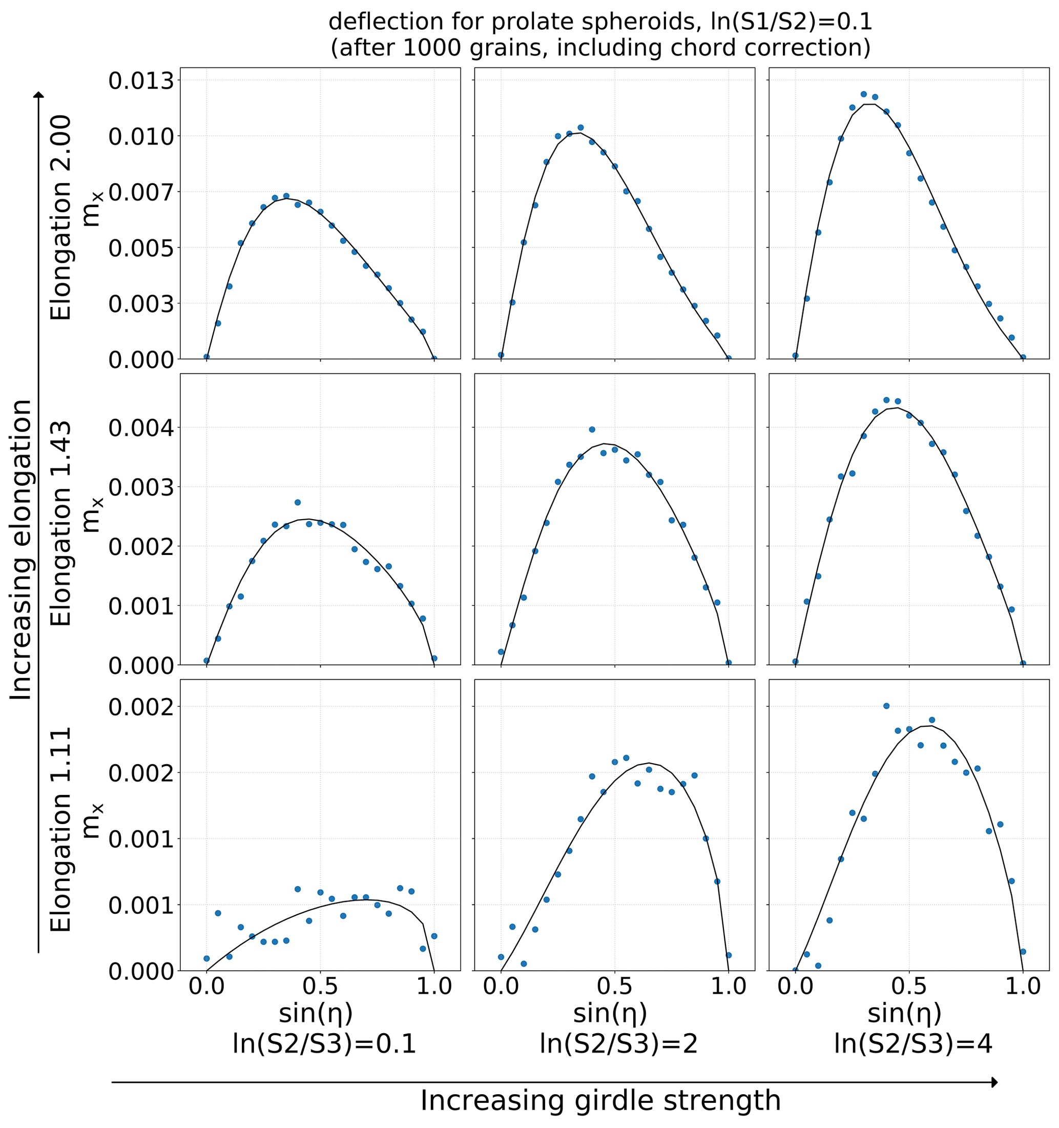
The three parameters of the diffusion pattern modeled with the 2D Gaussian on a sphere are the two widths (in the directions towards the flow, σ_x, and perpendicular to it, σ_y) and a single mean deflection towards the flow, m_x. The mean deflection in the perpendicular direction was zero for all cases that we chose to include in the final model (i.e., single-axis ellipsoids for particle shape and selected crystal fabric configurations). Because we mainly simulate small deflections (ignoring the long tails), we simulated the 2D Gaussian in Cartesian coordinates and then projected that to the sphere with an inverse stereographic projection. The three quantities were fitted to the following functions of angle η of the initial photon direction with respect to the ice flow for simulations with a fixed number of 1000 crystal crossings.

$$\begin{array}{}\text{(15)}& {\displaystyle }{m}_x& {\displaystyle }=\mathit{\alpha }\cdot \arctan (\mathit{\delta }\cdot \sin \mathit{\eta }\cos \mathit{\eta })\cdot \exp (-\mathit{\beta }\sin \mathit{\eta }+\mathit{\gamma }\cos \mathit{\eta })\text{(16)}& {\displaystyle }{\mathit{\sigma }}_x& {\displaystyle }=A_x\cdot \exp (-B_x\cdot [\arctan \left(D_x\sin \mathit{\eta }\right){]}^{C_x})\text{(17)}& {\displaystyle }{\mathit{\sigma }}_y& {\displaystyle }=A_y\cdot \exp (-B_y\cdot [\arctan \left(D_y\sin \mathit{\eta }\right){]}^{C_y})\end{array}$$

These functions were found to describe all considered crystal realizations with only 12 free parameters (A_x..D_x, A_y..D_y and α..δ). Figure 11 shows the mean deflection for nine crystal configurations. Note that increasing elongation has a stronger effect compared to a strengthening fabric, i.e., increasing the value of the Woodcock parameter $\ln (S_{\mathrm{2}}/S_{\mathrm{3}})$.

Figure 11 Deflection m_x as described in the text as a function of opening angle to the flow for a number of crystal configurations. The black curves were fitted through the blue simulated points using the functional form introduced in Eq. (17). Note the different ordinate scales per row.

6.2 Applying diffusion patterns in photon propagation

During photon propagation simulation, directions are only updated upon scattering. To minimize the additional computational burden, the new birefringence anisotropy is discretized and also evaluated only at the scattering sites. This requires scaling the diffusion, deflection, and displacement derived from simulation through 1000 grains to the number of traversed grains between two scattering sites. This introduces a new model parameter, the average grain size, and also requires taking into account the different average crystal chord lengths as a function of propagation direction (as described in Rongen, 2019), further increasing the importance of elongation over fabric.

The grain size distribution, which is the size distribution of ice mono-crystals, defines the distance between interface crossings. As would be expected from a diffusion process and was confirmed in simulation, the deflection scales linearly and the diffusion scales with the square root of the number of traversed grains n (${\mathit{\sigma }}_{x,y}\propto \sqrt{n}$ and m_x∝n). The overall ice diffusion strength, including both Mie scattering and the birefringence-induced diffusion, has previously been measured to great accuracy. To decouple the fitting of anisotropy properties from this overall ice, the effective scattering Mie coefficient was reduced by the amount resulting from the birefringence-induced light diffusion assuming on average isotropic photon directions.

Updating not only a photon's direction with deflection due to birefringence, but also the photon coordinates (as it shifts transversely with respect to straight-path expectation) at the next Mie scattering site, improves the agreement with data in the final fit. Due to the simple physics of cumulative photon deflections, the effect can be simulated at a small additional computational cost and with no additional parameters. Assuming without loss of generality that all birefringence deflections happen at constant distance interval Δl and that these can be sampled from the same distribution (which depends on the initial photon direction), as the individual and even final calculated deflections are very small, we can express the new photon direction n and coordinates r after N deflections as

$$\begin{array}{}\text{(18)}& {\displaystyle }\mathit{n}={\mathit{n}}_{\mathrm{0}}+\sum _{i=\mathrm{1}}^N\mathrm{\Delta }{\mathit{n}}_i,\text{(19)}& {\displaystyle }\mathit{r}=\sum _{i=\mathrm{1}}^N{\mathit{n}}_i\cdot \mathrm{\Delta }l=\mathrm{\Delta }l\cdot N\cdot {\mathit{n}}_{\mathbf{0}}\cdot +\mathrm{\Delta }l\cdot \sum _{i=\mathrm{1}}^N\sum _{j=\mathrm{1}}^i\mathrm{\Delta }{\mathit{n}}_j.\end{array}$$

The second term in each of the two expressions above describes a cumulative direction change δn and relative coordinate update δr, respectively (we note that the total distance traveled is $L=\mathrm{\Delta }l\cdot N$). We can now calculate that in the limit of large N we get

$$\begin{array}{}\text{(20)}& {\displaystyle }\langle \mathit{\delta }\mathit{r}\rangle =\langle \mathit{\delta }\mathit{n}\rangle {\displaystyle \frac{L}{\mathrm{2}}},\text{(21)}& {\displaystyle }\langle \mathrm{\Delta }(\mathit{\delta }\mathit{r}-\mathit{\delta }\mathit{n}{\displaystyle \frac{L}{\mathrm{2}}}{)}^{\mathrm{2}}\rangle =\langle \mathrm{\Delta }(\mathit{\delta }\mathit{n}{)}^{\mathrm{2}}\rangle \cdot {\displaystyle \frac{L^{\mathrm{2}}}{\mathrm{12}}},\text{(22)}& {\displaystyle }\langle \mathrm{\Delta }(\mathit{\delta }\mathit{r}-\mathit{\delta }\mathit{n}{\displaystyle \frac{L}{\mathrm{2}}})\cdot \mathrm{\Delta }\left(\mathit{\delta }\mathit{n}\right)\rangle =\mathrm{0}.\end{array}$$

Δ in the equations above is the variation (difference) from the mean of the quantity immediately following in brackets. These equations indicate that the coordinate update δr can be sampled from a distribution with a mean given by the first equation (which could be approximated by propagating the photon half the distance with initial direction vector and the other half with the final direction vector) and variance given by the second equation. Because there is no correlation between the residual in the variance and the deflection vector, as shown by the third equation, the variance can be sampled using the already tabulated birefringence parameters independently from sampling the variance of the deflection vector.

6.3 Fitting to flasher data

Besides the anisotropy direction already discussed in Sect. 4.2, the model described above requires four parameters to specify a birefringence anisotropy realization: crystal size and elongation and the two Woodcock parameters $\ln S_{\mathrm{1}}/S_{\mathrm{2}}$ and $\ln S_{\mathrm{2}}/S_{\mathrm{3}}$. Additionally allowing for a correction to the previously established total absorption and scattering coefficients adds two more parameters. As minimizing all six parameters for all 100 depth layers in the ice model is not computationally feasible, we need to simplify the model by identifying some parameters which are either depth-independent or have a small effect on the data–simulation agreement.

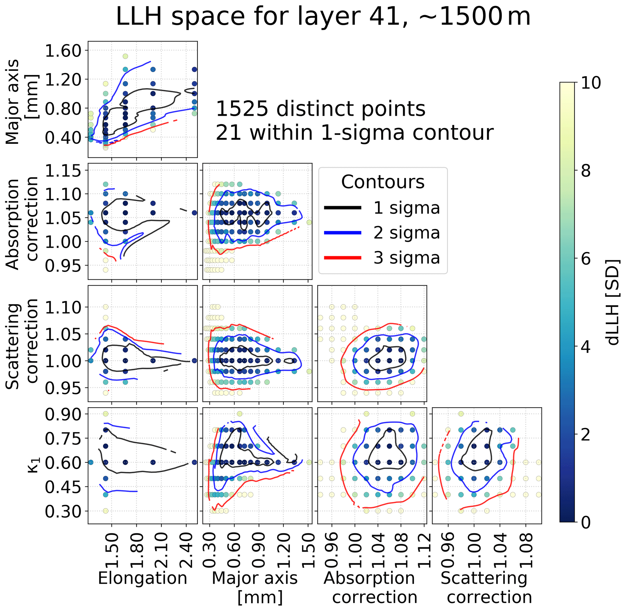
Figure 12 Log-likelihood (LLH) space, where each point quantifies the agreement of a simulation with a set of assumed parameter values against data, for one ice layer and a subset of parameters. Each panel shows a marginalized 2D space, each point being a simulated ice realization, color-coded by its LLH distance from the best fit. In this example, the absorption anisotropy (κ₁) is a free parameter (corresponding to the final model). This example is particularly detailed and is used to understand the behavior of the pre-fits. In particular, note the strong degeneracy in crystal elongation and size (parameterized as the scale of the major axis). Near-spherical crystals yield similar results to larger, more elongated realizations. The final fit for size, scattering, and absorption correction as performed for all layers generally contains around 100 tested realizations per layer.

This is done through pre-fits, which either vary all parameters for a single exemplary layer or fit the depth dependence of a single parameter while keeping all other parameters fixed. The required pre-fits, as well as the final depth evaluation, were performed following the method described in Aartsen et al. (2013c) and summarized in Sect. 3.3. This primarily entails minimizing the summed LLH comparing the single-LED data set (where all 12 LEDs were flashed one at a time on all in-ice DOMs) with the full photon propagation simulation of these events taking into account precisely known DOM orientations as measured in Chirkin et al. (2021). Fits for individual layers were carried out by only including LEDs situated within the considered (tilt-corrected) ice layer in the LLH summation. This method offers a reduced depth resolution compared to Aartsen et al. (2013c) but reduces computation time while making use of the full data. An example LLH space at a depth of ∼1500 m is shown in Fig. 12. During the pre-fits the following behavior was noted: given a girdle fabric ($\ln (S_{\mathrm{1}}/S_{\mathrm{2}})\ll \ln (S_{\mathrm{2}}/S_{\mathrm{3}})$), the actual fabric strength has a small effect and cannot be distinguished by the data. Accordingly the fabric has been fixed to values as measured in the deepest sections of the South Pole Ice Core SPC14 (Voigt, 2017) ($\ln (S_{\mathrm{1}}/S_{\mathrm{2}})=\mathrm{0.1}$ and $\ln (S_{\mathrm{2}}/S_{\mathrm{3}})=\mathrm{4}$). The fit is largely degenerate in crystal elongation and size, with small, near-spherical crystals yielding similar results to larger, more elongated realizations. Thus, the elongation was fixed to 1.4, which is a good fit at all layers and is a reasonable value given the largest value measured in the deepest parts of SPC14 (∼1.24) and the observed trend of increasing elongations up to that depth (Alley et al., 2021).

Fitting the remaining parameters (absorption and scattering corrections and crystal size) for all layers yields a significant improvement as seen, for example, in the average light curves in Fig. 6 (birefringence-only line). The best fit still features clearly visible discrepancies, such as an elevated intensity in the peak region in the case of propagation along the flow direction and too little intensity in the peak region in the case of propagation perpendicular to the flow direction. Problematically, the crystal sizes required to obtain this result are on the order of 0.1 mm and as such far smaller than expected from the overlapping SPC14 depths (Alley et al., 2021).

After thoroughly checking both the assumptions and implementation of the birefringence model, it was decided to reintroduce scattering as well as absorption anisotropy, both following the formalism of Chirkin (2013d), into the fit. As would be expected from the timing behavior, the fit does not make use of the scattering anisotropy, but surprisingly the absorption anisotropy is mixed into the birefringence model with a significant nonzero contribution. The fitted strength of the absorption anisotropy is nearly depth-independent with a directional modulation of the absorption coefficients by a factor of 2.45. This means a departure from a first-principles model but was adopted for its improvement in data–simulation agreement. After including the absorption anisotropy, absorption and scattering corrections and the crystal size were again fitted for all layers.

7 Resulting ice model

Figure 13 depicts the best-fit stratigraphy of grain sizes. The overall grain size of ∼1mm and the increase in size at larger depths, where ice crystals are generally larger, are as generally expected and measured in glaciology (e.g., Laurent et al., 2004; Alley et al., 2021). In addition an anticorrelation between crystal size and impurity concentrations, as mapped by optical properties, can be observed. This follows the expectation that impurity-related processes such as impurity drag hinder grain growth (e.g., Durand et al., 2006). As noted previously, the fit is largely degenerate in elongation and size. As a result the overall size scale is somewhat unconstrained. Repeating the fit under the assumption of an elongation of 1.7 instead of 1.4, for example, results in 26 % larger circle-equivalent diameters on average.

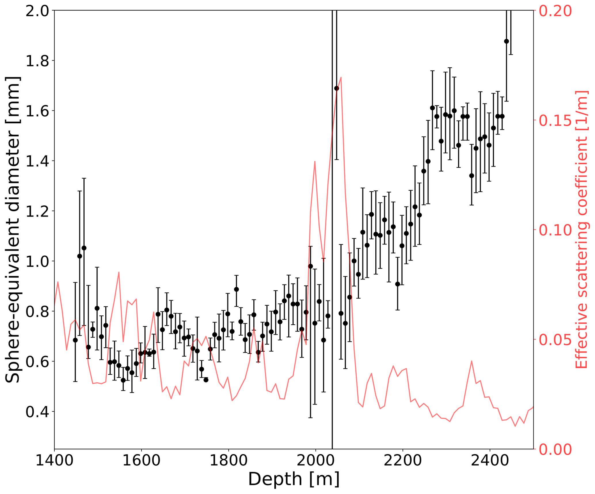
Figure 13 Best-fit crystal sizes as deduced in this analysis. The sphere-equivalent diameter denotes the diameter of a sphere with volume equivalent to the fitted spheroid describing the average crystal size and elongation at each depth. Error bars denote the statistical uncertainty only.

Averaged over all instrumented depths, light diffusion in the birefringent ice polycrystal amounts to an effective scattering coefficient of $\mathrm{2.47}\times {\mathrm{10}}^{-\mathrm{2}}$ m⁻¹, accounting for ∼8.5 % of the total scattering present in the ice on average. The comparatively strong isotropizing effect of Mie scattering also explains why the intensity on the tilt axis is never fully depleted.

As shown in Fig. 6, the new model significantly improves in matching the flasher data light curves in terms of both timing and total intensity with regards to older models and overall achieves excellent data–simulation agreement. While these light curves only represent some of the full data, the average relative deviation of each model from the data in the plots as shown is 8.5 %, 3.3 %, and 2.4 % for the scattering-function-based model, the birefringence-only model, and after including the ad hoc absorption anisotropy, respectively.

Widespread application in physics analyses requires large-scale simulations and is still in preparation. Nevertheless, first tests employing the ice model in direct-fit reconstructions (Chirkin, 2013c) of high-energy events (Aartsen et al., 2013b) indicate that the improved data–simulation agreement seen in flasher data also translates to more accurate descriptions of neutrino events.

8 Outlook

The model presented here is the first time that the ice microstructure has been included in the modeling of ice optical properties at macroscopic scales. Due to the need to include absorption anisotropy in order to arrive at reasonable grain sizes, for which no first-principles explanation is known, there appear to be remaining additional physical effects not fully accounted for by the first-principles model. At this point it remains unclear whether the anisotropic Mie absorption is real or if it is an artifact from incomplete modeling of birefringence effects. It is currently assumed, for example, that the deduced ice crystal properties follow the same layer undulations as the other ice optical properties and are not simply a function of absolute depth. This assumption may be reevaluated in future works.

Inclusion of ice-intrinsic attenuation in the electromagnetic calculations in Sect. 5 may already change the overall diffusion patterns. In addition, birefringent materials also exhibit di-attenuation where the imaginary index of refraction is polarization- and direction-dependent (Grechushnikov and Konstantinova, 1988). The overall imaginary refractive index of ice is largely unknown (with upper limits derived from IceCube/AMANDA measurements as mentioned earlier; Ackermann et al., 2006) and di-attenuation of ice in the optical has, to our knowledge, not been studied at all. A first step in exploring these options will be to include per crystal (di-)attenuation in the electromagnetic modeling, with the complex refractive indices as free parameters and fitting required values given different assumptions on the crystal orientation fabric. Yet, since the ice-intrinsic absorption accounts for at most 10 % of the overall absorption and the fitted absorption anisotropy is stronger than that, di-attenuation is unlikely to fully explain the observed effect.

The only other known and currently neglected birefringence effect is photoelasticity. Photoelasticity describes the change in refractive index due to applied stresses and is a property of all dielectric media, including ice. Ice is anecdotally known (e.g., Hobbs, 2010) to exhibit strong photoelasticity compared to its intrinsic birefringence strength. Yet, the stress optical parameters have so far only been measured by Ravi-Chandar et al. (1994) for light of an unspecified wavelength at an unspecified temperature and only for light propagating along the c axis. Ravi-Chandar et al. (1994) arrived at a material fringe value of ∼67 kN m⁻¹. Taking this measurement at face value, unrealistically large internal stress of roughly 200 MPa would be required to match the unstressed difference in refractive index.

To investigate the potential relevance of photoelasticity for light diffusion in deep glacial ice, the first step will be to repeat the Ravi-Chandar et al. (1994) measurement and extend it to light propagating orthogonal to the c axis. If photoelasticity adds a significant contribution, it would allow the presented measurement to also probe the stress state of the sampled ice in addition to the already studied microstructure.

8.1 IceCube Upgrade

The IceCube Upgrade (Ishihara, 2021), planned for deployment in 2025/2026, marks the first extension of the IceCube detector. Over 700 additional modules, including a number of stand-alone calibration devices (Henningsen et al., 2020; Rongen and Chirkin, 2021), will be deployed on seven additional strings. Of particular interest for the anisotropy are 11 so-called pencil beam devices. They allow a laser-like beam to be directed in arbitrary directions, enabling sweeps over receiver directions. The birefringence-induced deflection yields a unique signature, where the emission direction of maximum received intensity is offset from the geometric direction to the receiver. Measuring sweeping profiles for several emitter–receiver pairs at different orientations will allow us to disentangle absorption and birefringence contributions to the anisotropy with high precision.

8.2 Borehole logging

The described measurement is particularly tailored to the IceCube experiment. Nevertheless, the optical anisotropy effect may still prove to be a useful tool for glaciology. As described by Rongen et al. (2020), most likely fabric-induced azimuthal anisotropy was also observed in the back-scattered intensity recorded by an optical dust logger deployed down the SPC14 drill hole.

To date, the measurement has only been described qualitatively. An accurate simulation of the back-scattering scenario would need to include a good model for the large-angle tail of the Mie scattering function, which is currently poorly constrained from IceCube data. Given a better understanding of back-scattering processes, for example derived using the pencil beam described above, optical logging of drill holes could become a complementary tool for fabric, crystal size, and elongation studies and find wider application in glaciology.

9 Conclusions

Measurements of ice optical properties in the context of the calibration of the IceCube Neutrino Observatory and its predecessor AMANDA offer unique insights into the properties of glacial ice. In the past, modeling and measurements focused on the impact of airborne impurities as deposited with the original snow accumulation on absorption and scattering and their stratigraphy. This, in particular, yielded the most stringent upper limit as compiled by Warren and Brandt (2008) on the absorption coefficient of pure ice, as measured in the deepest parts of the detector.

Here we have described the observation of an ice optical anisotropy, a direction-dependent intensity modulation aligned with the local ice flow axis. The effect has been identified to largely result from diffusion within the polycrystalline ice microstructure, resulting in a previously unknown optical effect: a slow but continuous deflection towards the normal vector of the girdle plane of the crystal orientation fabric. Combining prior knowledge about the crystal orientation fabric and average grain elongation as obtained from SPC14, the depth-dependent average crystal size has been fitted to IceCube LED calibration data. The resulting depth evolution conforms to the expectation of larger crystals at greater depth and an inverse correlation with impurity concentrations.

The first-principles birefringence explanation was not able to fully describe the experimental data. This has been improved upon by including ad hoc Mie absorption anisotropy, for which no first-principles explanation is known. The origin of this remaining discrepancy will hopefully be resolved using upcoming instrumentation in the IceCube Upgrade, modeling of ice-intrinsic di-attenuation, and future lab measurements regarding the photoelasticity of ice.

Overall the large variety of measurements performed in close vicinity to the Amundsen–Scott South Pole Station (optical data from IceCube and its upcoming detector upgrade, the SPC14 ice core, ground-penetrating radar data from PolarGap, Forsberg et al., 2015; GPS stake field fields, Lilien et al., 2018) make the geographic South Pole a unique laboratory for comparative measurements. Yet to date, the overlap in sampled depth between SPC14 and IceCube is unfortunately too small to allow for quantitative comparison. This may be resolved by future drilling projects such as a potential deployment of the Rapid Access Ice Drill (RAID) (Goodge et al., 2021).

Appendix A: Sampling c-axis distributions from the eigenvalues of ice fabric orientation tensors

Table A1 Conceptual overview of different constituents considered as part of the ice optical modeling. For details on the behavior of different impurities see Ackermann et al. (2006) and He and Price (1998). The polycrystalline microstructure leading to asymmetric diffusion is newly considered in this work.

One can describe the crystal orientation fabric of N c axes, measured in an ice sample, by N unit vectors n_i, with components n_ix,n_iy, and n_iz. Note that n_i is equivalent to −n_i as the vector can be chosen to point along either direction of the axis. By convention n_i is chosen to point upward. This ensemble of vectors can be represented via the following matrix (Scheidegger, 1965).

$$\begin{array}{}\text{(A1)}& a=\left[\begin{array}{ccc}\sum n_{ix}^{\mathrm{2}}& \sum n_{ix}\cdot n_{iy}& \sum n_{ix}\cdot n_{iz}\\ \sum n_{iy}\cdot n_{ix}& \sum n_{iy}^{\mathrm{2}}& \sum n_{iy}\cdot n_{iz}\\ \sum n_{iz}\cdot n_{ix}& \sum n_{iz}\cdot n_{iy}& \sum n_{iz}^{\mathrm{2}}\end{array}\right]\end{array}$$

The normalized form $A=a/N$ is called the second-order orientation tensor. It was introduced in glaciology through Gödert and Hutter (1998). A has three eigenvectors and three corresponding eigenvalues S₁, S₂, and S₃, with $S_{\mathrm{1}}+S_{\mathrm{2}}+S_{\mathrm{3}}=\mathrm{1}$.

The axes of the coordinate system in which the c axes are evaluated can be chosen such that the x axis points along the mean c-axis direction $\sum {\mathit{n}}_i/N$, that the z axis points along the pole to the best-fit girdle to the distribution (see Woodcock, 1977), and that the y axis is orthogonal to the other two. In this case the coordinate axes are the eigenvectors, $S_j={\sum }_i{n}_{ij}^{\mathrm{2}}$, and the eigenvalues follow a strict ordering such that $S_{\mathrm{1}}\ge S_{\mathrm{2}}\ge S_{\mathrm{3}}$.

A perfectly uniform girdle or single-pole fabric features the following relations between the eigenvalues.

• uniform: $S_{\mathrm{1}}\approx S_{\mathrm{2}}\approx S_{\mathrm{3}}\approx \mathrm{1}/\mathrm{3}$

• single pole: $S_{\mathrm{1}}\approx \mathrm{1};S_{\mathrm{2}}\approx S_{\mathrm{3}}\approx \mathrm{0}$

• girdle: $S_{\mathrm{1}}\approx S_{\mathrm{2}}\approx \mathrm{0.5};S_{\mathrm{3}}\approx \mathrm{0}$

Woodcock (1977) realized that many commonly encountered fabric states can be visualized in a 2D plot, as only two of the three eigenvalues are independent. He suggested the representation where the abscissa is given as $\ln (S_{\mathrm{2}}/S_{\mathrm{3}})$ and the ordinate is given as $\ln (S_{\mathrm{1}}/S_{\mathrm{2}})$. In this representation uniform c-axis distributions are found at the origin of the plot. The distance from the origin $C=\ln (S_{\mathrm{1}}/S_{\mathrm{3}})$ is called the strength parameter. Girdle fabrics are found to the lower right, while single-pole fabrics reside to the upper left. The type of fabric can also be quantified by the so-called Woodcock shape parameter $K=\ln (S_{\mathrm{1}}/S_{\mathrm{2}})/\ln (S_{\mathrm{2}}/S_{\mathrm{3}})$. Large K values denote a single-pole fabric. K values smaller than 1 denote a girdle fabric. Figure A1 presents the fabric versus depth evolution as measured at the geographic South Pole in this representation.

Figure A1 Fabric versus depth trajectory as measured in the SPC14 ice core. Individual c-axis distributions at example depths are shown superimposed in the Schmidt equal-area projection. The ice features a prominent girdle fabric at the overlapping depths instrumented by IceCube starting at ∼1450 m. Adapted from Voigt (2017).

Neither the orientation tensor nor its eigenvalues retain the full information on the ensemble of underlying c axes. Thus, an assumption on the functional form of the fabric has to be made when trying to sample a distribution. Here we focus on describing random, girdle, and single-pole distributions, as well as combinations of these, as those are the types most commonly encountered in ice fabric measurements, with SPC14 in particular featuring a very strong girdle fabric.

The book Statistical analysis of spherical data by Fisher et al. (1987) gives a good overview of commonly used probability density functions (PDFs) for directional data. Of the presented PDFs the Watson (1965) distribution seems most applicable for our case due to the following.

1. It can represent both unimodal and single-pole as well as rotational symmetric girdle data.

2. An (approximate) parameter estimation exists based on eigenvalues alone.

In its standardized form the PDF, evaluated on a spherical coordinate system with the polar angle θ and the azimuth angle ϕ, has only one free parameter κ and is given as

$$\begin{array}{}\text{(A2)}& f(\mathit{\theta },\mathit{\varphi })=C_{\mathrm{w}}\exp (\mathit{\kappa }\cdot {\cos }^{\mathrm{2}}\mathit{\theta })\sin \mathit{\theta },\end{array}$$

with the normalization constant

$$\begin{array}{}\text{(A3)}& C_{\mathrm{w}}=\mathrm{1}/\left(\mathrm{4}\mathit{\pi }\underset{\mathrm{0}}{\overset{\mathrm{1}}{\int }}\exp \right(k\cdot u^{\mathrm{2}}\left)\mathrm{d}u\right).\end{array}$$

In the following, the Python package available at https://github.com/duncandc/watson_distribution (last access: 20 December 2023) is used to sample from the Watson distribution. Alternatively, the sampling approach described in Fisher et al. (1987) may be used.

At κ=0 the direction distribution is perfectly uniform. For positive κ the distribution is bimodal in vector space, which is equivalent to a single-pole distribution in axis space, and has the highest probability at the poles. For negative κ values the distribution is girdle with the directions equally distributed around the Equator.

Best and Fisher (1986) showed that for a purely single-pole distribution the κ parameter can be estimated from the eigenvalues as

$$\begin{array}{}\text{(A4)}& \mathit{\kappa }=\left\{\begin{array}{ll}\mathrm{3.75}\cdot (\mathrm{3}\cdot S_{\mathrm{1}}-\mathrm{1}),& \frac{\mathrm{1}}{\mathrm{3}}\le S_{\mathrm{1}}\le \mathrm{0.34}\\ -\mathrm{5.95}+\mathrm{14.9}{S}_{\mathrm{1}}+\frac{\mathrm{1.48}}{\mathrm{1}-S_{\mathrm{1}}}-\frac{\mathrm{11.05}}{S_{\mathrm{1}}^{\mathrm{2}}},& \mathrm{0.34}<S_{\mathrm{1}}\le \mathrm{0.64}\\ -\mathrm{7.96}+\mathrm{21.5}\cdot S_{\mathrm{1}}+\frac{\mathrm{1}}{\mathrm{1}-S_{\mathrm{1}}}-\mathrm{13.25}\cdot S_{\mathrm{1}}^{\mathrm{2}},& S_{\mathrm{1}}>\mathrm{0.64},\end{array}\right.\end{array}$$

while for a purely girdle fabric the κ parameter can be estimated as

$$\begin{array}{}\text{(A5)}& \mathit{\kappa }=\left\{\begin{array}{ll}\frac{\mathrm{1}}{\mathrm{2}\cdot S_{\mathrm{3}}},& \mathrm{0}\le S_{\mathrm{3}}\le \mathrm{0.06}\\ \mathrm{0.961}-\mathrm{7.08}\cdot S_{\mathrm{3}}+\frac{\mathrm{0.466}}{S_{\mathrm{3}}},& \mathrm{0.06}<S_{\mathrm{3}}\le \mathrm{0.32}\\ \mathrm{3.75}\cdot (\mathrm{1}-\mathrm{3}\cdot S_{\mathrm{3}}),& \mathrm{0.32}<S_{\mathrm{3}}\le \frac{\mathrm{1}}{\mathrm{3}}.\end{array}\right.\end{array}$$

For ice fabrics, the plane of girdle c axes shall intersect the poles, where the c axes of a single-pole distribution are also found. As such the directions sampled from girdle Watson distributions are rotated by 90^∘. Due to the underlying rotational symmetry the eigenvalues of the resulting Watson distributions follow a strict relation.

$$\begin{array}{}\text{(A6)}& \begin{array}{rlrl}{S}_{\mathrm{1}}& =S_{\mathrm{2}}& \text{ \& }& S_{\mathrm{3}}=\mathrm{1}-\mathrm{2}\cdot S_{\mathrm{1}}\text{ for a girdle Watson}\\ S_{\mathrm{2}}& =S_{\mathrm{3}}& \text{ \& }& S_{\mathrm{1}}=\mathrm{1}-\mathrm{2}\cdot S_{\mathrm{2}}\text{ for a unimodal Watson}\end{array}\end{array}$$

Obviously no single Watson distribution can describe an arbitrary set of eigenvalues with $S_{\mathrm{1}}\ne S_{\mathrm{2}}\ne S_{\mathrm{3}}$. This is achieved by combining directions sampled from a girdle and a unimodal Watson distribution.

Figure A2 Example c-axis distributions in Schmidt equal-area projection generated using the described method.

Given a sample of c axes from a girdle Watson distribution with eigenvalues S_ig and a sample of c axes from a unimodal Watson distribution with eigenvalues S_iu, as well as a relative fractional contribution of the girdle sample f_g to the total sample, the eigenvalues of the combined sample S_i are given by $S_i=f_g\cdot S_{ig}+(\mathrm{1}-f_g)\cdot S_{iu}$ The combination of f_g, S_1g, and S_2u which yields the desired eigenvalues S₁, S₂, and S₃ is found by solving the equation system S_i, which has been simplified using the relations in Eq. (A6):

$$\begin{array}{}\text{(A7)}& \begin{array}{rl}{S}_{\mathrm{1}}& =f_g\cdot S_{\mathrm{1}g}+(\mathrm{1}-f_g)\cdot (\mathrm{1}-\mathrm{2}\cdot S_{\mathrm{2}u}),\\ S_{\mathrm{2}}& =f_g\cdot S_{\mathrm{1}g}+(\mathrm{1}-f_g)\cdot S_{\mathrm{2}u},\\ S_{\mathrm{3}}& =f_g\cdot (\mathrm{1}-\mathrm{2}\cdot S_{\mathrm{1}g})+(\mathrm{1}-f_g)\cdot S_{\mathrm{2}u}.\end{array}\end{array}$$

The third equation is not independent since $S_{\mathrm{1}}+S_{\mathrm{2}}+S_{\mathrm{3}}=\mathrm{1}$. Thus further information is needed to be able to constrain the variables. To fulfill the assumption that S_u is unimodal and single-pole and S_g is girdle one can further constrain $\mathrm{1}/\mathrm{3}<S_{\mathrm{1}g}<\mathrm{0.5}$ and $\mathrm{0}<S_{\mathrm{2}u}<\mathrm{1}/\mathrm{3}$. For cases in which the system is still underconstrained one can, for example, further demand that $S_{\mathrm{2}g}=S_{\mathrm{2}u}=S_{\mathrm{1}g}$ (equivalent to $S_{\mathrm{1}u}+S_{\mathrm{3}g}=\mathrm{1}$) so that both distributions have an equal spread around the girdle plane. The solution is then given as

$$\begin{array}{}\text{(A8)}& \begin{array}{rl}{f}_g& =\mathrm{0.5}\cdot (\mathit{ϵ}-\mathrm{4}{S}_{\mathrm{1}}-\mathrm{2}{S}_{\mathrm{2}}+\mathrm{3}),\\ S_{\mathrm{1}g}& ={\displaystyle \frac{\mathrm{2}{S}_{\mathrm{1}}}{-\mathit{ϵ}+\mathrm{4}{S}_{\mathrm{1}}+\mathrm{2}{S}_{\mathrm{2}}+\mathrm{1}}},\\ S_{\mathrm{2}u}& ={\displaystyle \frac{\mathit{ϵ}-\mathrm{2}{S}_{\mathrm{2}}-\mathrm{1}}{\mathrm{2}\cdot (\mathit{ϵ}-\mathrm{4}{S}_{\mathrm{1}}-\mathrm{2}{S}_{\mathrm{2}}-\mathrm{1})}},\end{array}\end{array}$$

with $\mathit{ϵ}=\sqrt{\mathrm{16}\cdot S_{\mathrm{1}}^{\mathrm{2}}+\mathrm{16}{S}_{\mathrm{1}}\cdot (S_{\mathrm{2}}-\mathrm{1})+(\mathrm{2}{S}_{\mathrm{2}}+\mathrm{1}{)}^{\mathrm{2}}}$. From these one can derive the Watson parameters κ using the approximations as given in Eqs. (A4) and (A5).

To verify and visualize the success of the presented sampling approach, c-axis distributions according to a number of combinations of $\ln (S_{\mathrm{1}}/S_{\mathrm{2}})$ and $\ln (S_{\mathrm{2}}/S_{\mathrm{3}})$ have been generated as shown in Fig. A2. The sampled c-axis distributions yield eigenvalues which are accurate to within the approximation of the parameter estimation for the Watson distributions and sufficient for most applications.

Note that by design the c-axis distributions for intermediate fabric states do not contain a single elliptical distribution but a rotationally symmetric girdle and a circular single pole. This seems suitable for our application to ice fabrics. In very deep glacial ice where the fabric slowly evolves from girdle to single pole, experimental distributions such as published by Weikusat et al. (2017) indeed show the described superposition and not an elliptical distribution usually sketched for these eigenvalues.

Appendix B: Sampling surface orientations from an ellipsoid

As the average grain shape deviates from a sphere, the encountered distribution of face orientations depends on the photon direction. Assuming that the face orientation of a solid, tessellated into elongated polyhedra, to be described by the surface orientation density of an ellipsoid describing the average grain shape, one can sample the distribution as follows.

The surface of an ellipsoid is defined by the equation

$$\begin{array}{}\text{(B1)}& f(x^{\prime },y^{\prime },z^{\prime })={\displaystyle \frac{{x^{\prime }}^{\mathrm{2}}}{a^{\mathrm{2}}}}+{\displaystyle \frac{{y^{\prime }}^{\mathrm{2}}}{b^{\mathrm{2}}}}+{\displaystyle \frac{{z^{\prime }}^{\mathrm{2}}}{c^{\mathrm{2}}}}=\mathrm{1},\end{array}$$

where a, b, and c are the dimensions of the major and minor axes. The normal vector on any point of the surface is given by the gradient

$$\begin{array}{}\text{(B2)}& \mathrm{\nabla }f=[\mathrm{2}\cdot {\displaystyle \frac{x^{\prime }}{a^{\mathrm{2}}}},\mathrm{2}\cdot {\displaystyle \frac{y^{\prime }}{b^{\mathrm{2}}}},\mathrm{2}\cdot {\displaystyle \frac{z^{\prime }}{c^{\mathrm{2}}}}].\end{array}$$

For a given set of azimuth and zenith angles, the coordinates on a unit sphere ($x,y,z$) and on the ellipsoid ($x^{\prime },y^{\prime },z^{\prime }$) are given as

$$\begin{array}{}\text{(B3)}& {\displaystyle }x& {\displaystyle }=\sin \mathit{\theta }\cdot \cos \mathit{\varphi }\text{ and }{x}^{\prime }=a\cdot x,\text{(B4)}& {\displaystyle }y& {\displaystyle }=\sin \mathit{\theta }\cdot \sin \mathit{\varphi }\text{ and }{y}^{\prime }=b\cdot y,\text{(B5)}& {\displaystyle }z& {\displaystyle }=\cos \mathit{\theta }\text{ and }{z}^{\prime }=c\cdot z.\end{array}$$

Substituting the ellipsoid surface position into Eq. (B2) the surface normal at this position is then

$$\begin{array}{}\text{(B6)}& \mathit{n}=\left[{\displaystyle \frac{\mathrm{2}}{a}}\cdot \sin \mathit{\theta }\cdot \cos \mathit{\varphi },{\displaystyle \frac{\mathrm{2}}{b}}\cdot \sin \mathit{\theta }\cdot \sin \mathit{\varphi },{\displaystyle \frac{\mathrm{2}}{c}}\cdot \cos \mathit{\theta }\right].\end{array}$$

One can now sample these gradients with angles chosen to be uniform on a sphere. As the surface density per solid angle of an ellipsoid is different from a sphere, the relative surface density,

$$\begin{array}{}\text{(B7)}& \begin{array}{rl}{\mathit{\mu }}_{(x,y,z)}& =\left|\right|\mathrm{d}{S}^{\prime }\left|\right|/\left|\right|\mathrm{d}S\left|\right|\\ & =\sqrt{(ac\cdot y{)}^{\mathrm{2}}+(ab\cdot z{)}^{\mathrm{2}}+(bc\cdot x{)}^{\mathrm{2}}},\end{array}\end{array}$$

has to be applied as a weighting factor, where the maximum weighting factor is given as

$$\begin{array}{}\text{(B8)}& {\mathit{\mu }}_{\max }=max(ac,ab,bc).\end{array}$$

Instead of weighting, one can also employ a rejection sampling with an acceptance probability of $\mathit{\mu }/{\mathit{\mu }}_{\max }$.

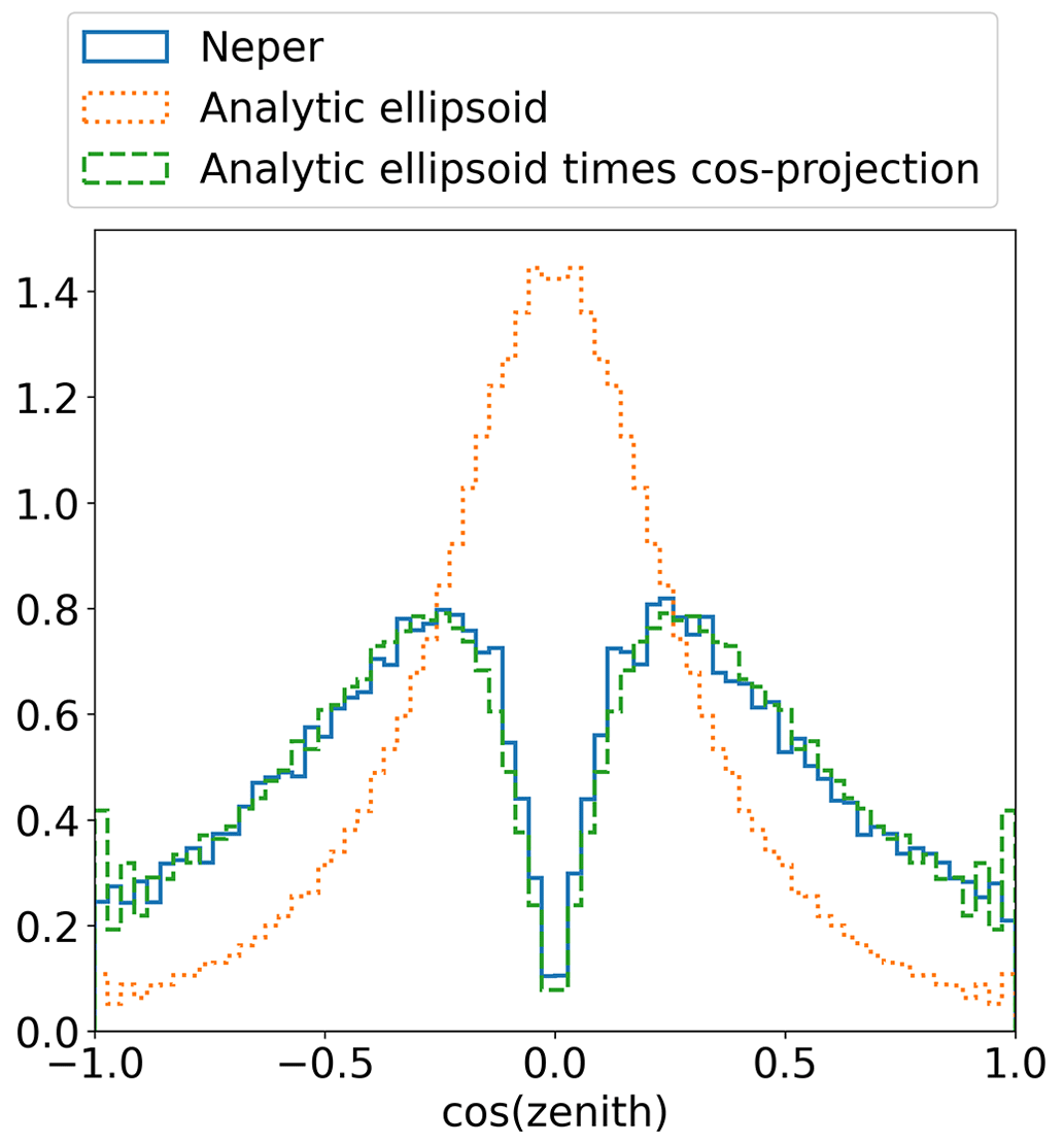
Figure B1 Ellipsoid surface sampling for an ellipsoid with unity minor axes and a major axes of two along the z axis. Green: analytic cos (θ) distribution of face normal vectors. Red: analytic cos (θ) distribution weighted by the encounter probability, given by the scalar product with a photon propagating along z. Blue: encounter probability as found in a Neper crystal tessellation simulation when tracing photons along vertical lines.

In addition to the distribution of face orientations, the distribution of face orientations actually encountered by a photon can be obtained by weighting the distribution of face orientations with the scalar product of the photon's propagation vector and each face normal vector. The probability of encountering a given plane is therefore simply the projected area relative to the incident light.

Figure B1 shows the cos (θ) distribution of (encountered) face normal vectors for a spheroid with elongation 2, which has the major axis aligned with the z axis. The distribution is compared to a crystal-like Voronoi tessellation generated with Neper and assuming the same mean elongation. Lines have been traced through the tessellation, identifying grain boundary encounters and computing their incidence angles. The distributions are found to be indistinguishable, confirming that the ensemble of polyhedra faces follows the average ellipsoid.