the Creative Commons Attribution 4.0 License.
the Creative Commons Attribution 4.0 License.
 | 20 Feb 2024
Bayesian physical–statistical retrieval of snow water equivalent and snow depth from X- and Ku-band synthetic aperture radar – demonstration using airborne SnowSAr in SnowEx'17
Siddharth Singh
Michael Durand
Edward Kim
Ana P. Barros
A physical–statistical framework to estimate snow water equivalent (SWE) and snow depth from synthetic aperture radar (SAR) measurements is presented and applied to four SnowSAR flight-line data sets collected during the SnowEx'2017 field campaign in Grand Mesa, Colorado, USA. The physical (radar) model is used to describe the relationship between snowpack conditions and volume backscatter. The statistical model is a Bayesian inference model that seeks to estimate the joint probability distribution of volume backscatter measurements, snow density and snow depth, and physical model parameters. Prior distributions are derived from multilayer snow hydrology predictions driven by downscaled numerical weather prediction (NWP) forecasts. To reduce the signal-to-noise ratio, SnowSAR measurements at 1 m resolution were upscaled by simple averaging to 30 and 90 m resolution. To reduce the number of physical parameters, the multilayer snowpack is transformed for Bayesian inference into an equivalent one- or two-layer snowpack with the same snow mass and volume backscatter. Successful retrievals meeting NASEM (2018) science requirements are defined by absolute convergence backscatter errors ≤1.2 dB and local SnowSAR incidence angles between 30 and 45∘ for X- and Ku-band VV-pol backscatter measurements and were achieved for 75 % to 87 % of all grassland pixels with SWE up to 0.7 m and snow depth up to 2 m. SWE retrievals compare well with snow pit observations, showing strong skill in deep snow with average absolute SWE residuals of 5 %–7 % (15 %–18 %) for the two-layer (one-layer) retrieval algorithm. Furthermore, the spatial distributions of snow depth retrievals vis-à-vis lidar estimates have Bhattacharya coefficients above 94 % (90 %) for homogeneous grassland pixels at 30 m (90 m resolution), and values up to 76 % in mixed forest and grassland areas, indicating that the retrievals closely capture snowpack spatial variability. Because NWP forecasts are available everywhere, the proposed approach could be applied to SWE and snow depth retrievals from a dedicated global snow mission.
- Article
(7334 KB) - Full-text XML
- BibTeX
- EndNote


The seasonal snowpack plays a critical role in climate and weather variability due to its role in the surface energy budget on account of its high albedo and in the surface water budget as temporary storage of frozen precipitation in the cold season until it melts in the warm season and becomes available as runoff. The water stored in the snowpack is measured by the snow water equivalent (SWE), the depth of liquid water per unit area that would be released if the snowpack were to melt completely. It is the product of the specific gravity of snow with respect to water () and the depth of the snowpack (SD). To map SWE in the cold season is to map snow water resources. To map onset of melt and snow wetness is to map the timing and geography of snow water resources availability. Climate variability and change with increasing air temperature, shifts in atmospheric moisture convergence patterns, and increases in the frequency of extreme events are already causing significant changes in frequency, patterns, and timing of seasonal snow accumulation and melt with severe implications for water and food security in addition to cascading economic and ecosystem impacts (Huang and Swain, 2022; Musselman et al., 2021; Sturm et al., 2010).
The need to capture snowpack heterogeneity and dynamics tied to weather, climate, land cover, and landform variability remains a chief challenge to developing a snow observing system at the spatial and temporal scales required to answer water cycle science questions and for societal decision-making. The potential for systematic snowpack monitoring in remote regions has long been investigated, including the integration of remote sensing measurements and physical models (e.g., (Martinec, 1991; Mote et al., 2003; Bateni et al., 2015; Li et al., 2017; Kim et al., 2019; Cao and Barros, 2023a). Assimilation of radiance or backscatter is most powerful with a time series of observations. Time series observations are available presently from tower measurements, albeit at the point scale of the tower footprint (see summary by Tsang et al., 2022), and do not capture the large joint spatial and temporal variability of snowpacks from local to regional scales depending on weather and climate, landform, land use, and land cover. Frequent spatial observations are required for this purpose. Airborne observations can be used for mapping but typically occur once or twice during a winter season and over limited areas. A dedicated satellite mission is necessary to acquire time series of measurements globally.
Presently, advances in radar technology and retrieval algorithms (Tsang et al., 2022), and especially the demonstrated capabilities of NewSpace satellite missions (Villano et al., 2020), make high spatial resolution of synthetic aperture radar (SAR; tens of meters) Earth observations from space feasible in contrast to the challenges faced in the past (Rott et al., 2012). During the SnowEx'17 field campaign (Kim et al., 2017), a comprehensive data set consisting of airborne dual-frequency SAR (X- and Ku-band synthetic aperture radar) backscatter measurements using the SnowSAR instrument (Macedo et al., 2020), the Airborne Snow Observatory (ASO, Painter et al., 2018), and a plethora of high-quality ground-validation measurements of snowpack properties and ancillary data (Table 1) offers an unprecedented opportunity to investigate the full potential of SAR toward developing the next generation of retrieval algorithms.
Due to the highly nonlinear snow physics and the time-varying stratigraphy of snowpacks, radiance or backscatter measurements depend on the vertical structure of snowpack physical properties such as snow density, snow temperature, and snow grain size in addition to SWE and snow depth. Because the number of observations is smaller than the number of parameters required to solve the inverse problem, retrieval of SWE and snow depth is an underdetermined estimation problem. This challenge can be addressed using a physical–statistical approach for retrieval. Physical–statistical approaches combine physical process models with a Bayesian statistical framework to inform how geophysical states and parameters relate to measurements by obeying fundamental physical constraints (Berliner, 2003; Lowman and Barros, 2014). In this paper, we propose and evaluate a general physical–statistical framework to retrieve SWE from SnowSAR measurements across a heterogeneous landscape during SnowEx'17.
2.1 Forward simulation – from SWE to backscatter
The advantage of SAR technology is the high spatial resolution of its measurements, which is necessary to capture the spatial heterogeneity of snowpack physical processes (e.g., Mendoza et al., 2020; Manickam and Barros, 2020) as demonstrated in forward simulations. Cao and Barros (2020, 2023a; hereafter CB20 and CB23) demonstrated the utility of a multilayer snow hydrology (MSHM) coupled with a radiative transfer model (RTM) forced by high-resolution operational numerical weather prediction (NWP) model forecasts to capture the seasonal hysteresis behavior of the seasonal snowpack at Grand Mesa and Senator Beck in Colorado against Sentinel-1 C-band measurements.
The MSHM is a physically driven snow hydrology model that simulates the evolution of snowpack physical properties including detailed stratigraphy (Kang and Barros, 2012a, b; CB20). During snowfall events, fresh snow is added to the top layer of the snowpack until a threshold accumulation is met and a new layer forms. The RTM used here is MEMLS3&a (Microwave Emission Model of Layered Snowpacks) adapted to include backscattering by Proksch et al. (2015). MEMLS is a physically driven radiative transfer model that takes snowpack characteristics as inputs and simulates its microwave emission for a frequency band with four polarizations – HH, VV, HV, and VH (originally proposed by Wiesmann and Mätzler, 1999). To estimate total scattering, ground backscatter σbkg must be modeled as well, as described below.
Figure 1 illustrates the various backscatter mechanisms contributing to total backscatter (σtotal) in active microwave measurements represented in MEMLS3&a (the RTM): volume backscatter (σvol) from the multiple interactions of the incoming radar signal within the snowpack and the backscatter at the snowpack–air interface (σsurf) and at the snowpack–ground interface including interactions with submerged vegetation and litter (σbkg). In forested areas, additional backscatter mechanisms are associated with the multiple bounce pathways among tree canopies, intercepted snow, tree trunks, and snowpack. Depending on viewing geometry (flight path and incidence angle), σtotal measurements from areas without trees in regions of mixed land cover can include significant contributions from trees along the grassland–forest transitions.
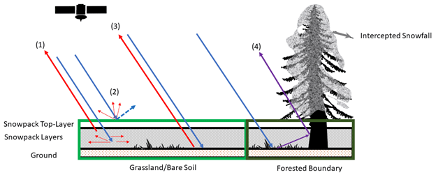
Figure 1Scattering mechanisms for grassland submerged by snow and snowpack over bare soil or rock: (1) volume backscatter σvol, (2) surface backscatter σsurf, (3) background backscatter at the snow–ground interface σbkg, and (4) snowpack–ground–canopy–tree trunk interactions at forested boundaries. Red arrows (1), (2), and (3) are resolved in the retrieval applications demonstrated here.
CB23 used the coupled MSHM-MEMLS in forward mode to predict Sentinel-1 C-band volume backscatter σvol without calibration or nudging of ground observations without bias and within ±2.5 dB at 90 m resolution across terrain slopes in the 10–52∘ range for barren land, alpine grass and shrubs, and in forested areas with snow-free canopy at the beginning of spring in the Senator Beck Basin in Colorado. They estimated σbkg as the average of Sentinel-1 measurements for snow-free conditions. Cao and Barros (2023b) modified MEMLS3&a to include double-bounce effects among snowpack and vegetation (MEMLS-V) and retrieved σbkg from total backscatter σtotal measurements in mixed land cover using simulated annealing. Their estimates are consistent with CB23, suggesting the potential to simplify the inverse problem of estimating snowpack physical properties from total backscatter measurements in mixed land cover and further simplify the physical–statistical retrieval framework proposed here, although further evaluation is necessary.
2.2 Physical–statistical retrieval
For retrieval in a Bayesian framework, the probability of the retrieved geophysical variable x (the inferred posterior distribution) is conditional on the a priori knowledge of the variable x (the prior distribution), indirect measurements D, and a physical model M(η) (e.g., the snow radiative transfer algorithm in this case), with physical parameters η (including x) and statistical error parameters ζ. The joint probability distribution of M, D, η, and ζ can be written as follows:
The first term to the right-hand side of Eq. (1) is the backscatter data model, the second term is the prior of the backscatter, and the third term is the prior of the snowpack physical parameters (including snow depth and snow density, etc.) with statistical error parameters. Assuming that the measurements do not depend on the physical parameters, the model does not depend on the statistical error parameters, and the physical parameters and the statistical parameters are independent, Eq. (1) can be revised to read
Finally, in the context of specific measurements y with known uncertainty described by P(y)
The physical model M and P(y) are invariant, and assuming that we have a good understanding of the statistical errors, then Eq. (3) can be further simplified as follows:
In the context of Bayesian inference the goal is to maximize P(η|y), the posterior probability of physical parameters conditional on measurements informed by the a priori parameter probabilities P(η). This implies maximizing the second term in Eq. (4), the posterior of the backscatter conditional on physical parameters η, minimizing the difference between measurements y with a known error covariance matrix Σy and model predictions M(η). For multiple concurrent measurements, P(y|η) can be described by a multivariate normal distribution,
where N is the number of measurements at a given location and time (e.g., backscatter at different frequencies as in Durand and Liu (2012).
Pan et al. (2023, hereafter P23) adapted a Bayesian retrieval algorithm previously developed to estimate SWE from passive microwave measurements (Pan et al., 2017, hereafter P17) to active microwave, hereafter referred to as Base-AM. The snow radiative transfer algorithm in Base-AM is MEMLS, and the semi-empirical Dobson model is used to estimate the soil dielectric constant as a function of soil moisture and soil texture (Dobson et al., 1985; Hallikainen et al., 1985). A Monte Carlo Markov Chain (MCMC) iterative algorithm (Metropolis et al., 1953) is used to sample from P(η|y) starting from initial values and using the likelihood ratio criteria to achieve convergence. In this work, realistic snowpack predictions from MSHM-MEMLS are used to define the prior distributions of parameters and constrain the Bayesian retrievals: y represents the SnowSAR backscatter measurements, and η represents all model parameters and geophysical variables including SWE, SD, and snow density.
3.1 Study area and ancillary data
The study region is Grand Mesa, Colorado, a plateau that is 2000 m above adjacent low-lying areas and is surrounded by ridges up to 500 m in elevation (as depicted in Fig. 2). Grand Mesa has an alpine climate, experiencing snowfall throughout the year except during the months of July and August. Land cover is heterogeneous with grasslands in the west and a mix of evergreen and deciduous forest to the east. Numerous wetlands are widespread across the Mesa, especially in the transition from grassland to forest. The land cover data were obtained from the National Land Data Assimilation System (NLDAS). The data sets were upscaled to 90 m using nearest-neighbor interpolation to support retrievals at 90 m resolution (see Sect. 4). NLDAS is used to determine land cover type in the snow hydrology model. North American Land Change Monitoring System (NALCMS) is used to upscale the evaluation data. Hourly albedo is derived from NLDAS at 12.5 km resolution. A summary of all the data sets used in this study is available in Table 1.
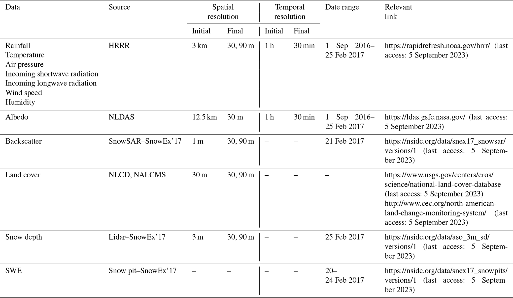
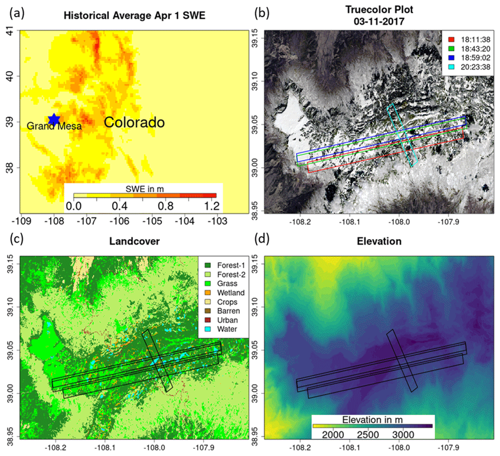
Figure 2Study area in Grand Mesa, Colorado. (a) Location of Grand Mesa in Colorado, with historical 1 April SWE average as base map. (b) Paths of four SnowSAR SnowEx'17 flights on 21 February 2017, with true-color image obtained from Landsat on 11 March 2017 as the base map. (c) Land cover of the study region. Forest-1 indicates needleleaf forests. Forest-2 indicates broadleaf forests. (d) Digital elevation map of the study region.
3.2 Atmospheric forcing
Numerical Weather Prediction (NWP) outputs are used as the atmospheric forcing for the snow hydrology model and to set up boundary conditions. Previously, CB20 and CB23 relied on HRRR (high-resolution rapid refresh) hourly forecasts at 3 km and downscaled it to 90 m in Grand Mesa. Here, the same data set was independently downscaled to 30 m as well. The HRRR data set is produced by National Ocean and Atmospheric Agency (NOAA) by hourly assimilation of observations at 13 km resolution (Benjamin et al., 2016; Table 1). Hourly atmospheric forcing was linearly interpolated to 30 min temporal resolution used in the snow hydrology model.
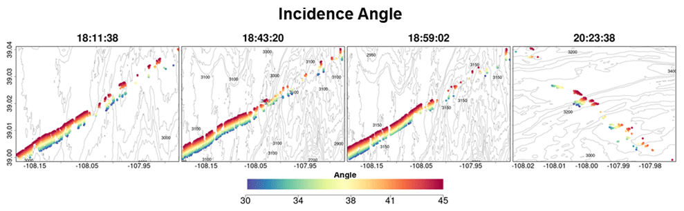
Figure 3Maps of incidence angles along SnowSAR flight paths on 21 February 2017 during SnowEx'17.
3.3 SnowSAR backscatter
During SnowEx'17, airborne microwave backscatter measurements were made in Grand Mesa on 21 February 2017 at 1 m resolution (Table 1). The SnowSAR instrument is a dual-frequency (X and Ku band) radar. A total of six flight lines were completed, two short ones on sloped densely forested terrain and four long lines on the plateau. Here, only the four flight lines on the plateau are used for analysis (Figs. 2 and 3). The flights are between 18:00 and 21:00 GMT (12:00–15:00 MST). SnowSAR data quality control measures included filtering based on aircraft attitude (there were line segments with turbulence), beam incidence angle or antenna pattern, and signal-to-noise ratio of the backscatter coefficients. Processing of the original airborne SAR measurements and quality control indicate that only the co-pol X-band HH- and VV-pol and Ku-band VV-pol measurements are adequate for retrieval. Geolocation was verified against corner reflector targets and geographic features and found to be very robust. The SnowSAR data were upscaled to 30 and 90 m resolution by simple averaging of all SnowSAR measurements within each pixel.
3.4 Validation data
Lidar snow depth. The Airborne Snow Observatory (ASO) lidar measurements of snow depth at 3 m resolution across Grand Mesa are available for SnowEx'17 on 25 February, thus 4 d after the SnowSAR flights (Painter et al., 2018; Table 1). There were no significant snow storms or strong winds in that period, except for about 3 mm of rainfall for less than 1 h on 24 February. These data are used to examine the distribution of retrieved snow depths, that is indicative of the spatial heterogeneity of the snowpack, and the relative absolute differences between lidar measurements and retrieval of snow depth, that are indicative of local retrieval errors. The lidar data were upscaled to 30 and 90 m using simple averaging (e.g., Fig. 4a). There can be large snow depth underestimation errors associated with upscaled lidar retrievals along the edges of forests where the snow depth is underestimated consistent with previous work (e.g., Deems et al., 2013; Jacobs et al., 2021). Given the expect measurement uncertainty on the order of 10–20 cm in Grand Mesa, which is amplified by microtopography, lidar pixels with snow depth shallower than 20 cm are not considered for evaluation.
Snow pit SWE. Multiple snow pits were excavated during the SnowEx'17 field campaign across Grand Mesa (Table 1). Due to the small number of snow pit measurements along the SnowSAR flight lines on 21 February, snow pit measurements on 20–24 February were considered for evaluation assuming that in the absence of snowstorms or other weather events the snowpack does not change significantly during the 4 d period. Differences are expected at local places but the overall spatial trends should be maintained such as the west–east gradient in snow depth. The values of snow pit SWE are estimated using an average of the snow density measurements at different depths applied to the entire snow depth. Only pits in the non-forested areas were selected for evaluation (Fig. 4b).
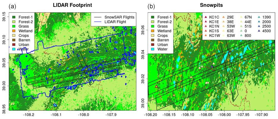
Figure 4(a) Flight footprint of the lidar instrument used to measure the snow depth during SnowEx'17. (b) Location of snow pits used to measure SWE 20–24 February 2017. The legend identifies SnowEx'17 pit IDs.
Simplicity and computational efficiency are desirable attributes for an operational algorithm that produces successful retrievals, here understood as meeting science uncertainty requirements and latency adequate to meet application needs defined by NASEM (2018). The retrieval methodology builds on existing and well-evaluated snow hydrology, radiative transfer, and physical–statistical models (CB20,CB23, P17, P23) previously reviewed in Sect. 2. A list of forcings and coupling variables and parameters among MSHM, MEMLS, and Base-AM is provided in Table 2.
Averaging is necessary to reduce the signal-to-noise ratio (SNR) in SnowSAR measurements at their native resolution (Sect. 3.3). Because the highest spatial resolution of available ancillary data sets is 30 m, the SnowSAR measurements were upscaled to 30 m to eliminate the need for interpolation and/or downscaling that would introduce further uncertainty. Following results by Manickam and Barros (2020), the algorithm was also applied at 90 m resolution consistent with the first scaling break identified in Sentinel-1 SAR backscatter. The implication of linear scaling behavior is that successful retrievals at 90 m resolution can subsequently be statistically downscaled with confidence, which has significant computational advantages. Further upscaling was not conducted because the number of pixels becomes very small given the available coverage of SnowSAR flights.
Table 2Input and output parameters from the three models in the SWE physical–statistical retrieval framework.
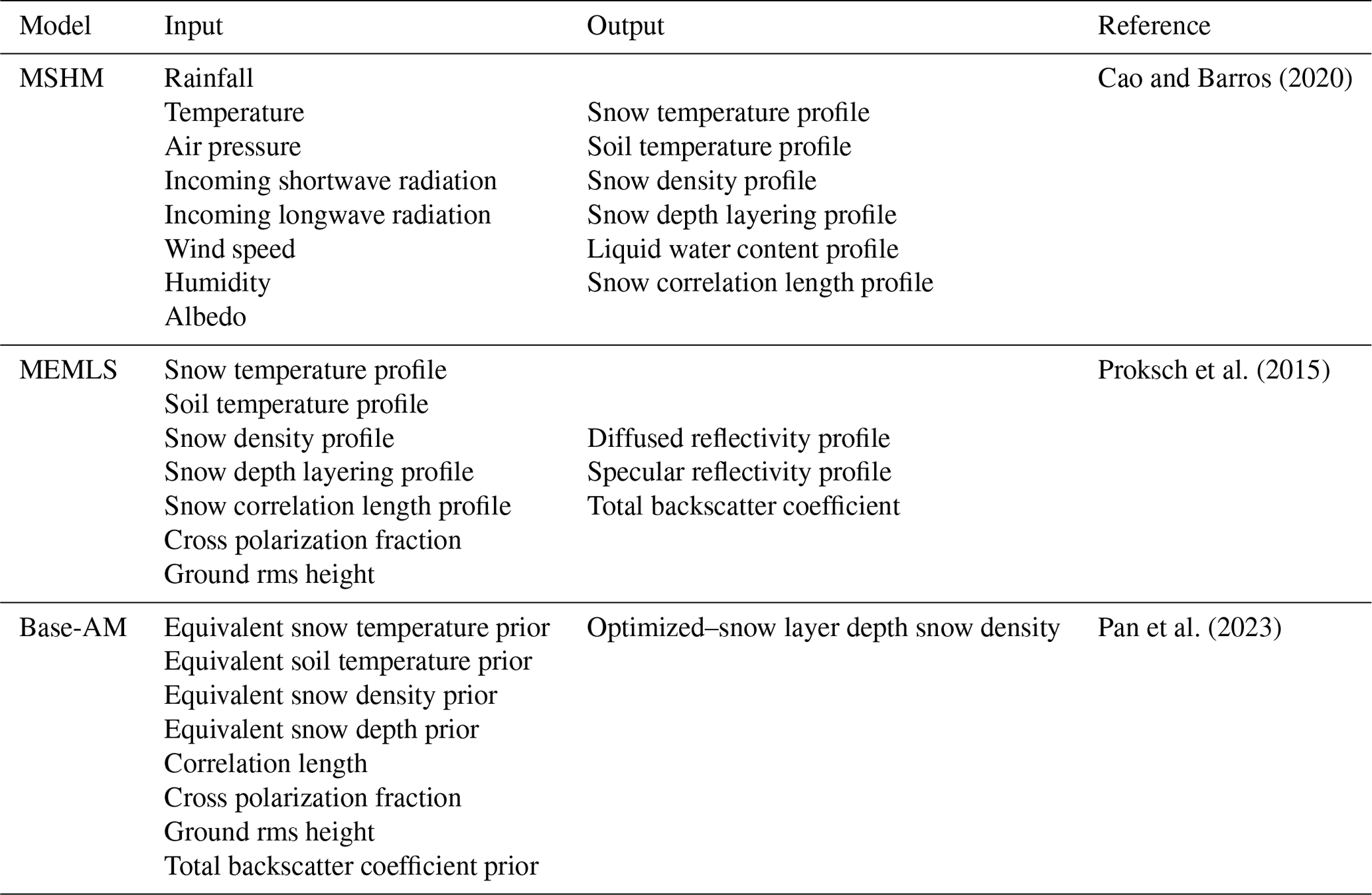
Figure 5 illustrates the retrieval workflow consisting of four main steps. Step 1 entrails snow hydrology simulation using MSHM to produce a layered snowpack and volume backscatter simulation using MEMLS (). Step 2 consists of Bayesian estimation of ground parameter priors that govern background backscatter σbkg using MEMLS assuming a very thin film of snow on the ground (1 mm SD) at the beginning of the accumulation season and estimation of the σbkg by subtraction of from SnowSAR total backscatter measurements . Step 3 is the determination of snowpack priors for Bayesian SWE retrieval using results step 1 and step 2. Step 4 is the Bayesian optimization of simulated to derive posterior distributions of SD and ρsnow for the one- and two-layer (1|2) equivalent snowpack and subsequent calculation of retrieved SWE posterior distributions.
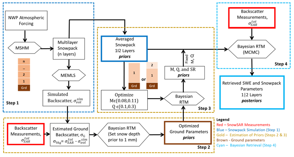
Figure 5Workflow of the SWE physical–statistical retrieval framework. NWP atmospheric forcings drive MSHM to determine priors for the Bayesian radiative transfer model (Base-AM) and synthetic backscatter for ground parameters. SnowSAR backscatter measurements are assimilated to determine the posterior distribution of the snowpack parameters.
4.1 Layered snowpack simulations (step 1)
Following the methodology presented in Sect. 2.1, MSHM was run for a full-year starting from snow-free conditions on 1 September 2016 using downscaled HRRR data as atmospheric forcing (Sect. 3.2) and a time step of 30 min. On the day of the SnowSAR flights, the snowpack physical properties predicted at times corresponding to each of the four flights are used to derive the 1|2 Layer equivalent snowpack properties used in the retrieval. The simulated volume backscatter () was estimated by specifying the cross-polarization fraction parameter Q=0.2 following CB20. This is an empirical coefficient that distributes the diffuse scattering into cross- and like-polarization components in MEMLS (Proksch et al., 2015).
In realistic layered snowpacks, stratigraphy (i.e., vertical heterogeneity) is a dominant feature of the density, temperature, microstructure, and dielectric properties (e.g., emissivity and reflectivity). The vertical structure of snow microstructure in MSHM is described using a parameterization of snow correlation length (lex) consistent with MEMLS formulation. Depending on the number of layers, this poses an undetermined problem as the number of measurements is equal to the number of frequencies and the number of polarizations available (typically two or three). For example, there are only four observations for a dual-frequency measurement with dual polarization. In contrast, the set of independent parameters per layer includes snow density, layer thickness, liquid water content, snow grain size or correlation length, temperature, reflectivity, and transmissivity.
While converting the multilayer snowpack to a single-layer model is the simpler path to address the undetermined inverse problem, fresh snowfall accumulation and snowpack crusting artifacts due to melt–refreeze cycles, as well as hardening by wind action, introduce strong density and grain size differences at the top of the snowpack. To capture this behavior, we implement and evaluate the retrieval algorithm for both one- and two-layer equivalent snowpacks derived from the layered snowpack simulated by MSHM. The equivalent one- or two-layered snowpack parameters for each pixel are obtained by matching SWE, snow depth (SD), and volume backscatter () of the simulated multilayer snowpack.
4.2 Ground and snowpack parameter priors (steps 2 and 3)
A first estimate of the σbkg is obtained by subtracting from SnowSAR X-band HH-pol measurements following Baghdadi et al. (2011), who found better performance among backscattering models for HH-pol against TerraSAR-X measurements. In Base-AM, σbkg depends on the effective soil moisture and soil surface roughness. To optimize these parameters, σbkg is used as an “observed” value. To simulate snow-free conditions, the snow depth is constrained to a maximum value of 1 mm in step 2. The cross-polarization fraction Q initially specified as Q=0.2 is optimized first and separately from other ground parameters in the third step of the retrieval algorithm (Fig. 5). The posterior distributions of the ground parameters in step 2 are used along with the 1|2 layer prior distributions and the SnowSAR measurements to estimate the posterior distributions of snow depth and snow density using the Base-AM framework (Fig. 5) and both X- and Ku-band VV-pol. SWE is subsequently derived from snow depth and snow density.
One-layer snowpack. The total snow depth and the averages of multilayered snowpack parameters are specified as the mean of the prior distribution for retrieval. Table 3 shows the range and standard deviation of the parameters.
Table 3Base-AM model input variance and range for the parameters prepared using MSHM multilayer snowpack parameters. The alphanumerical subscript in two-layer snowpack retrievals denotes layer number: 1 is the bottom layer, 2 is the top layer, avg represents the average of all MSHM multilayer parameter values in the corresponding one or two-layer snowpack. DZ is the MSHM snow depth.
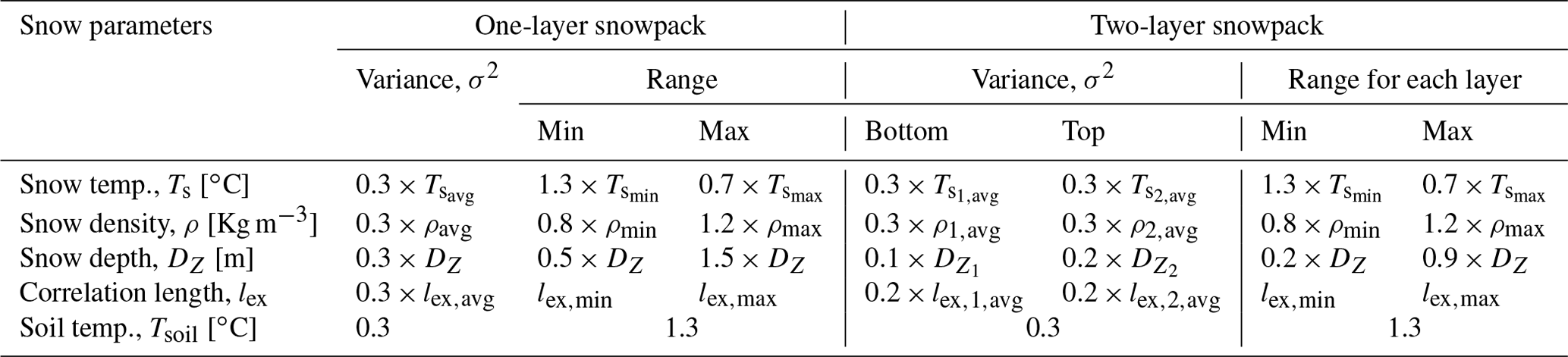
Two-layer snowpack. The average values of the snowpack physical properties for each layer are derived from the multilayer snowpack simulated by MSHM. The key requirement is to determine the depth of each one of the layers that best captures the snowpack vertical structure. Figure 6 shows MSHM simulated snowpack density profiles for each of the four SnowSAR flights. The shape of the profiles reflects the interplay between thermodynamic processes that change snow microstructure and dominate in the upper snowpack and mechanical consolidation processes that are dominant in the middle and lower layers. The snow depth point corresponding to the maximum change in snow density between adjacent layers in the multilayer snowpack is used here to divide the snowpack into two layers. Subsequently, the layer-depth-weighted average density, snow temperature, and correlation length of the MSHM multilayer snowpack is calculated for the corresponding depths of the two-layer equivalent snowpack (Table 3).
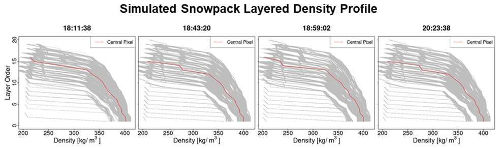
Figure 6Density profiles simulated by MSHM for all grassland pixels at 30 m resolution from the four SnowSAR flight paths. The density profile of the central pixel for each of the flights is marked in red. The snowpack layers are numbered from bottom to top tracking the evolution of simulated snowpack stratigraphy during the accumulation season. Note the significant difference between the top two to three layers and the deeper snowpack supporting the two-layer snowpack conceptual retrieval model.
4.3 Bayesian optimization (Step 4)
Realistic snowpack predictions from MSHM driven by weather forecasts (Step 1) are used to define the prior distributions of snowpack parameters and constrain Base-AM (Steps 2 and 3) to infer the posterior distribution of snowpack parameters given the SnowSAR backscatter measurements (Step 4) as discussed in Sect. 2.2.
The local mean of the posterior distribution for each parameter is hereafter referred to as the retrieval result for each pixel. SD retrievals are evaluated against lidar snow depth including spatial patterns and gradients and overall statistical structure using histograms. SWE retrievals derived from the posterior distributions of snow density and snow depth are evaluated against SWE measurements at snow pits (Sect. 3.4). Original lidar measurements were reprojected and coregistered with the SnowSAR retrievals. A comparative analysis was conducted to examine the dependence of retrievals on incidence angle, and the subgrid-scale variability was quantified in terms of the standard deviation of original lidar measurements within the upscaled pixel. The amplitude error metrics are the mean, standard deviation, and mean absolute relative error (MARE):
where O are observations and R are retrievals. The Bhattacharya coefficient (BC) is used to compare the spatial distributions of snow depth and backscatter. BC measures the similarity between two probability distributions p1 and p2 as follows (Bhattacharya, 1946):
Finally, among the 39 snow pits available for evaluation on 21 February, only 15 pits in open areas (i.e., grasslands) were retained for evaluation, and snow pits without SnowSAR measurements within a radius of 100 m were discarded.
5.1 Successful retrievals
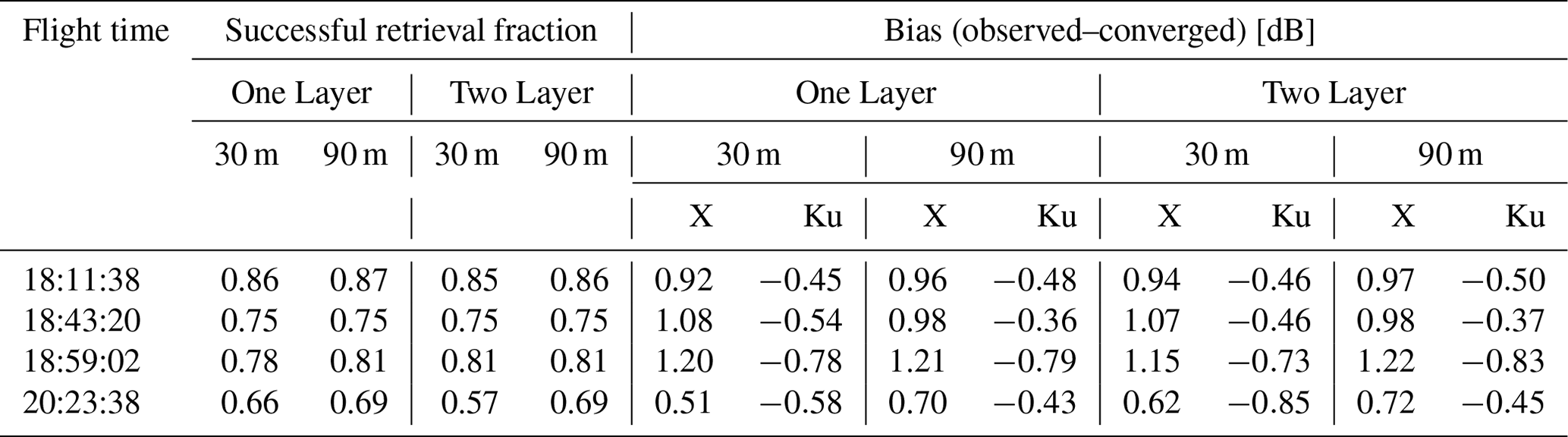
SnowSAR measurements are strongly affected by aircraft operations, viewing geometry that varies systematically along the flight path, resulting in amplitude artifacts amplified by landform and land cover heterogeneity. Even after separating homogeneous grassland pixels, there is contamination from multiple bounce artifacts at grassland–forest transitions and adjacent wetlands that cannot be resolved at 30 or 90 m resolution. Other errors embedded in the retrieval are associated with downscaling of HRRR forcings that produce biased snow priors, snow hydrology model structure, and errors tied to the background backscatter estimation. Combined, these errors compounded can lead to a weak convergence of the Bayesian optimization algorithm, resulting in large backscatter residuals. To account for these errors and meet NASEM (2018) science requirements, SnowSAR pixels for which the relative residual backscatter (RRB) between Base-AM simulated and SnowSAR measurements was greater than 30 % were identified as unsuccessful. In an operational context, these pixels would be flagged and identified as failed or highly uncertain retrievals. The successful retrieval fraction after restricting the range of incidence angles and imposing the RRB <30 % criterion is summarized in Table 4 for the four flights and for both 1|2 layer snowpack retrievals at 30 and 90 m resolution. Except for the later flight path over the predominantly forested areas in the eastern sector of Grand Mesa (Fig. 1), the fraction of successful retrievals by restricting the incidence angle and RRB varies between 75 % and 87 % across the four SnowSAR flights with a maximum absolute bias of 1.2 dB. Only figures with retrieval results at 30 m resolution are shown in the main text; retrieval results at 90 m resolution, as well as other supporting analysis, can be found in Appendix A.
Table 4Spatial bias between SnowSAR backscatter and converged backscatter from Base-AM for successful retrievals for grassland pixels at 30 and 90 m spatial resolution over each flight. Successful retrievals are for pixels with local incidence angles in the 30–45∘ range and relative residual backscatter (RRB) of less than 30 % for each of the four flights.
5.2 Retrieval skill
Figure 7 compares lidar snow depth (Fig. 7a) against colocated SnowSAR retrievals at 30 m for the SnowSAR flight at 18:11:38 GMT (GMT = MST+6). The SnowSAR retrievals for high incidence angles underestimate the lidar snow depth (orange and red points). Lemmetyinen et al. (2022) suggested a nominal incidence angle of 35–45∘ for retrievals, ensuring proper focusing and calibration of SnowSAR swaths. CB23 showed good skill in forward backscatter simulations for incidence angles as low as 30∘. Overall, the retrievals here also show very good performance for incidence angles between 30 and 45∘. Note, however, the large residuals for SnowSAR retrievals with high incidence angles (red and orange points in Fig. 7b) corresponding to lidar pixels with shallow snow depth (below the 1:1 line) and large subgrid-scale variability (orange and red points, Fig. 7c). Analysis for all flights at both 30 and 90 m resolution can be found in Appendix A (please see Figs. A1 and A2, similar to Fig. 7b, and Figs. A3 and A4, similar to Fig. 7c). Figure 7d, e, and f show the land cover, spatial distribution of subgrid standard deviation (SSTD), and absolute residual (retrieved–lidar) snow depth for the same flight. Along the edges of forest, the SSTD in the upscaled pixels is large due to high heterogeneity that cannot be resolved by the lidar fusion algorithm for snow depth retrieval (Painter et al., 2016). The red box identifies an area with complex grassland–forest boundaries (Fig. 7d) and high subgrid-scale variability (Fig. 7e), resulting in poor lidar estimates. The edge of wetlands also has comparatively higher residuals than completely homogeneous grasslands. This corresponds to the lidar pixels with SSTD >0.3 m (yellow, orange and red in Fig. 7c). Therefore, only lidar pixels with SSTD ≤0.3 m are used for assessment of retrievals.
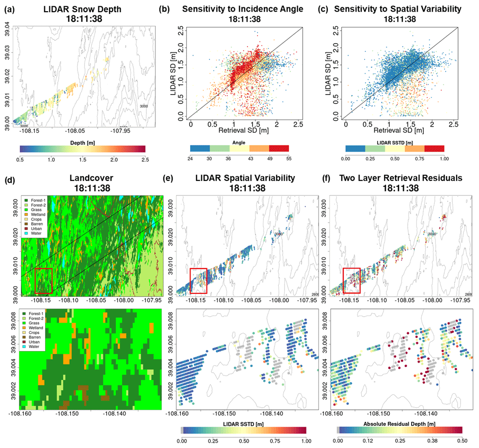
Figure 7(a) Snow depth measurements using airborne lidar on 25 February 17, 4 d after the SnowSAR flights. (b) Comparison between lidar snow depth and the two-layer retrieved snow depth from SnowSAR on 21 February 2017 at 18:11:38 GMT. The pixels are color-coded according to the SnowSAR incidence angle. Panel (c) is the same as (b) with pixels color-coded according to the subgrid-scale variability measured by standard deviation of lidar snow depth within the corresponding 30 m pixel. Pixels on the edge of forests and grasslands have higher subgrid-scale standard deviations (SSTDs). (d) Land cover distribution along the flight path; the bottom panel shows a zoomed-in view of the area in the red box. (e) Spatial distribution of upscaled lidar snow depth SSTD at 30 m; the bottom panel shows a zoomed-in view of the area in the red box. The edges of forests have higher SSTD due to errors in the lidar snow depth retrievals at high resolution. (f) Absolute residual between retrievals and lidar snow depth; the bottom panel shows a zoomed-in view of the area in the red box. Residuals equal to 0.5 m and above are grouped in the same category. The red box in panels (d), (e), and (f) delineates an area with large absolute residuals. Vegetation–snowpack backscatter interactions at the grassland–forest and grassland–wetland margins are not accounted for in the retrievals. Gray points in the central panel correspond to zero-depth lidar estimates due to errors in heterogenous land cover.
Figure 8 shows heatmaps (density maps) to compare successful retrievals against observed X- and Ku-band VV-pol total backscatter at 30 m resolution. There is good agreement between the two values for both the bands, especially in the −15 to −10 dB range, without significant differences between one- and two-layer snowpack retrievals. Note the positive bias in the case of X-band simulations compared to observations, whereas Ku-band simulations have a negative bias as quantified in Table 4. Overall, the retrievals at 90 m resolution show better agreement than those at 30 m resolution due to averaging (Fig. A5).
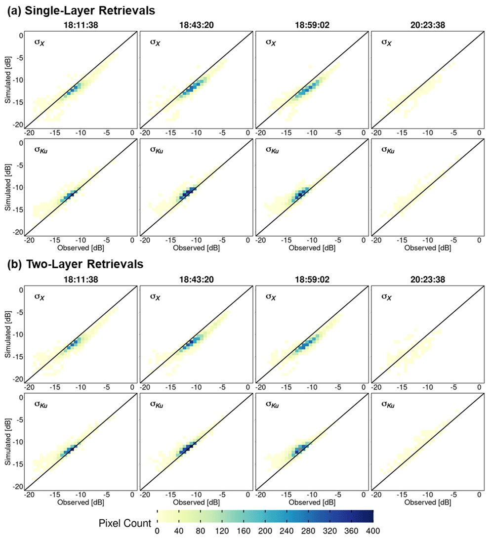
Figure 8Heatmaps of SnowSAR measurements (observed) versus retrievals (simulated) backscatter (σ) at 30 m resolution for X band (σX) and Ku band (σKu): (a) one-layer snowpack and (b) two-layer snowpack. Successful retrievals are for pixels with local incidence angles in the 30–45∘ range and relative residual backscatter (RRB) of less than 30 % for each of the four flights (see Table 4).
Maps of successful SWE retrievals for the four SnowSAR flight paths are shown in Figs. 9 and A6 at 30 and 90 m resolution, respectively. The retrievals capture the west–east gradient in SWE well and show realistic spatial variability across Grand Mesa. The very low SWE and shallower snow depths at the easternmost boundary of the flight lines are underestimates introduced by upscaling of the SnowSAR backscatter values where there are significant changes in topography at the edge of the plateau (see Fig. 2).
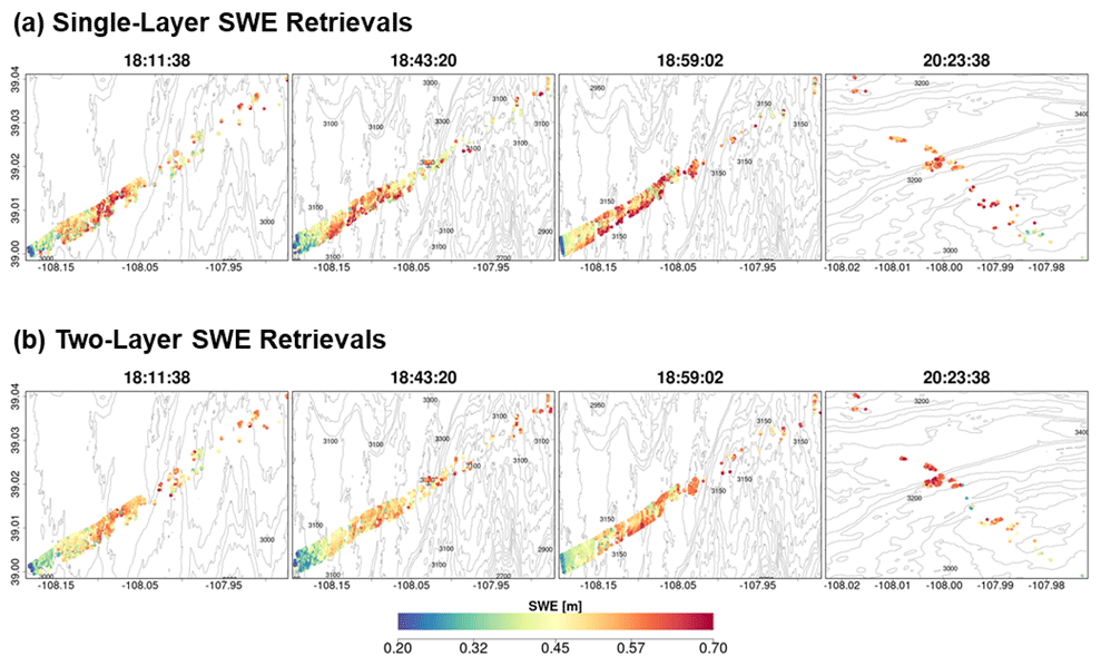
Figure 9Spatial distribution of successful SWE retrievals for one-layer (a) and two-layer (b) snowpacks in grassland pixels at 30 m resolution. Successful retrievals are for pixels with local incidence angles in the 30–45∘ range and relative residual backscatter (RRB) of less than 30 % for each of the four flights (see Table 4).
Heatmaps of total snow depth priors (MSHM-predicted snow depth) against lidar snow depth are shown in Figs. 10 and A7 at 30 and 90 m resolution and can be contrasted with heatmaps of total snow depth posteriors) against lidar snow depth in Figs. 11 and A8 using both one- and two-layer retrievals. Note the narrow range of the prior snow depths concentrated around 1.5 m and the positive bias relative to lidar. The posteriors show much wider range of variability and deeper snow consistent with the lidar data for both one- and two-layer retrievals, albeit with better agreement for the latter with high counts overlaying the 1:1 line at both spatial resolutions. This behavior is further confirmed by examining the snow depth histograms in Figs. A9 and A10. The retrievals capture the range of the lidar snow depths well for all flights, and there is a substantial improvement in the shape of the distributions as revealed by the heatmaps.
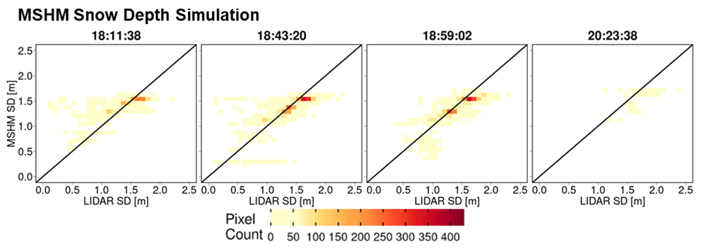
Figure 10Heatmap of lidar and MSHM-predicted snow depth priors at 30 m resolution using overlapping pixels from the MSHM and lidar. Only pixels with an incidence angle between 30 and 45∘ and moderate subgrid-scale variability of lidar snow depth (<0.3).
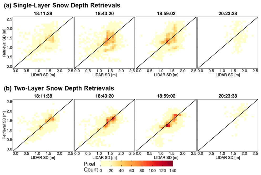
Figure 11Heatmap of lidar versus successful snow depth (SD) retrievals at 30 m resolution using overlapping lidar and retrieval pixels. Successful retrievals are for pixels with local SnowSAR incidence angles in the 30–45∘ range and relative residual backscatter (RRB) of less than 30 % for each of the four flights (see Table 4). Lidar SD in pixels with subgrid-scale variability corresponding to standard deviation of less than 0.3 m for the upscaled 90 m lidar pixel are not included.
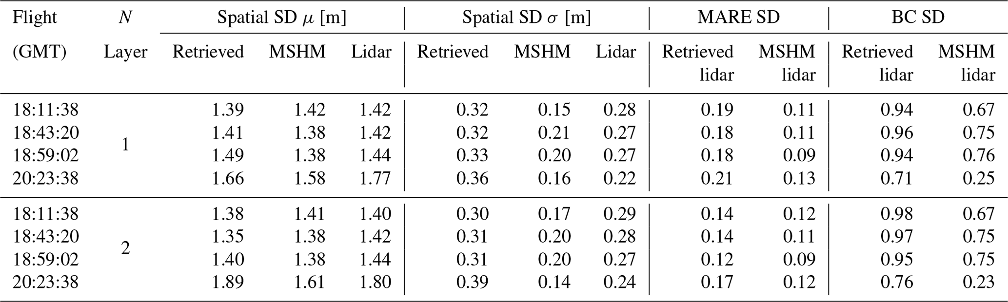
Quantitative assessment metrics are presented in Tables 5 and A1 for the comparison between various snow depth data sets at 30 and 90 m resolutions, respectively. The snow depth MARE is higher for the retrievals compared to the priors (MSHM) due to the fact that MARE is an effective metric capturing distance from the mean. CB20 showed that the MSHM simulated average snow mass accumulation at the Grand Mesa scale is within 10 % of observations at a monthly timescale in February 2017. The BC coefficients The BC coefficients of 0.95 and above at 30 m resolution indicate significant agreement between the shapes of the distributions at 0.95 or above at 30 m resolution using the two-layer retrievals for the west–east flights and 0.76 for the fourth flight at 20:23:38 GMT over the forested area. There is significant improvement relative to MSHM priors in the statistical similarity of the snow depth retrievals vis-à-vis the lidar data for all cases, and more so for the fourth flight over the forest. For snow depth, 30 m resolution and two-layer retrievals outperform the 90 m resolution and one-layer retrievals for all flights. This is explained in part by land cover classification errors that are smaller at 30 m. Figure A11 shows that the number of pixels where retrievals produce large mean absolute residuals is very small, and they are characterized by low confidence in the lidar estimates.
Table 5Summary of statistics and error metrics of the three snow depth (SD) data sets at 30 m resolution: lidar measurements, MSHM predictions, and successful SnowSAR retrievals for grassland pixels and subgrid-scale standard deviation (σ) of less than 0.3 m for the upscaled lidar pixel. MARE is the mean absolute relative error (Eq. 6), and BC is the Bhattacharya coefficient (Eq. 7). Here mean and standard deviation refer to the spatial distribution, unlike the prior mean and standard deviation used in Base-AM (Table 3). Successful retrievals are for pixels with local incidence angles in the 30–45∘ range and relative residual backscatter (RRB) of less than 30 % for each of the four flights (see Table 4).
Tables 6 and A2 summarize the average absolute relative errors between snow pits and SWE retrievals from all flights within 100 m of the snow pits. The results are significantly better for two-layer snowpack retrievals. The mean absolute relative errors at 30 m resolution are 0.22 and 0.13 for one-layer and two-layer snowpacks, respectively. The mean absolute relative errors at 90 m resolution are 0.2 and 0.12 for one-layer and two-layer snowpacks, respectively. There is a variable number of pixels used for the calculation of the error metrics for each snow pit, which in the case of 51S is so small that it suggests the pit is not in the flight path. The large errors for pits 4500, 44E, and 53W are attributed to very heterogeneous land cover including water and forest (4500) and proximity to roads (53W and 44E). After removing these snow pits in the central area marked in Fig. A12, the average absolute relative SWE residuals are 5 %–7 % (15 %–18 %) for the two-layer (one-layer) retrieval algorithm.
Table 6Evaluation of successful SWE retrievals at 30 m resolution against SWE at SnowEx'17 snow pits and retrieved snowpacks at 30 m resolution. All N pixels with centroids within 100 m of each snow pit are in the grasslands (according to the land cover data set at 30 m resolution; see Table 1). SD stands for snow depth. Italicized rows correspond to large local MARE (mean absolute relative error, Eq. 6).
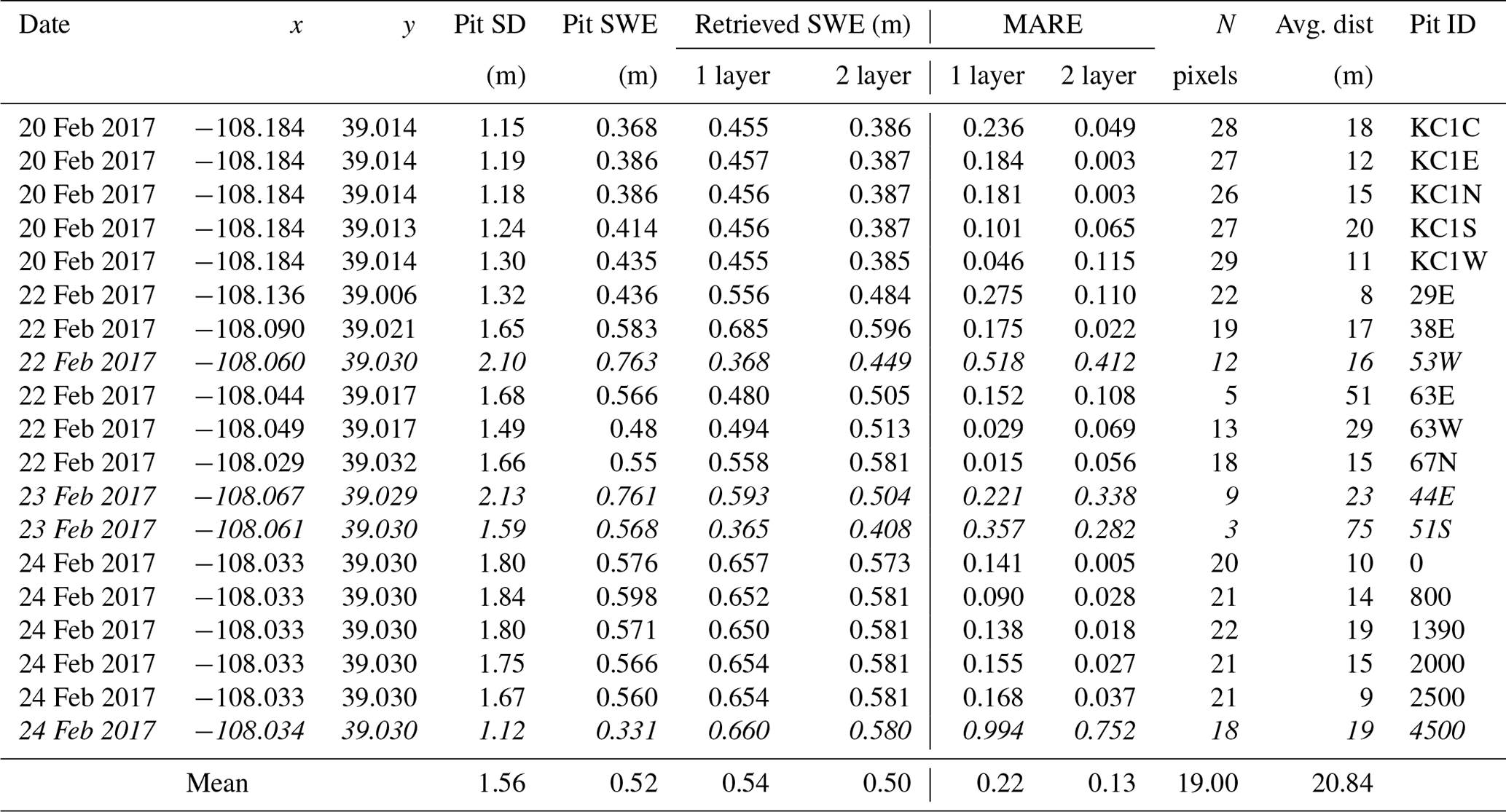
Finally, composite spatial maps of successful SWE retrievals from all flights overlain by the snow pit measurements between 20 and 24 February are shown in Fig. 12. Because of the different viewing geometries, retrievals between incident angles 30–35∘ for the flight path at 18:59:02 GMT in the composite of overlapping flight paths at 18:43:20 and 18:59:02 GMT were removed. Note the consistency between 30 and 90 m resolutions and the overall agreement between SWE at snow pits and SWE retrievals on the flight lines.
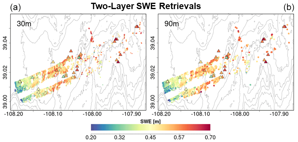
Figure 12Composite spatial distribution of SWE (two-layer retrievals) successfully retrieved at 30 m (a) and 90 m (b) resolution for grassland pixels for the four SnowSAR flights. Snow pits (20–24 February, Fig. 4, Table 6) are marked by triangles colored according to SWE. SnowEx'17 snow pit locations are marked by triangles and colored according to SWE. Successful retrievals are for pixels with local incidence angles in the 30–45∘ range and relative residual backscatter (RRB) of less than 30 % for each of the four flights (see Table 4). As two flights overlap, only retrievals with higher incidence angles are shown in the composite figure. Gray elevation contours are plotted every 100 m.
A Bayesian physical–statistical SWE retrieval framework leveraging prior work (CB20, CB23, P17, P23, Fig. 5) was applied to airborne X- and Ku-band measurements yielding robust results from multiple SnowSAR flights over grassland and mixed grassland and forest in Grand Mesa, Colorado. Prior distributions of snowpack parameters were obtained from a multilayer snow hydrology model with atmospheric forcing derived from operational NWP forecasts and analysis (CB20, CB23). In order to reconcile the number of independent measurements and physical constraints and reduce the number of snowpack parameters, snowpack stratigraphy was mapped into one-layer and two-layer snowpacks and then Bayesian inference using Base-AM was applied (P17, P23). The SnowSAR measurements were averaged to 30 and 90 m resolutions, and retrievals were conducted independently for every measurement pixel along the flight lines. Retrievals for measurements with convergence backscatter relative errors less than 30 % (±1.2 dB) and for incidence angles in the 30–45∘ range were considered successful over grasslands, corresponding to 75 %–87 % of all retrievals depending on the flight.
The retrievals, specifically the local means of the posterior distributions, were evaluated against the spatial distribution of lidar snow depth estimates up to 2 m and against snow pit SWE measurements up to 700 mm and snow depth up to 2.13 m. Since the lidar and snow pit measurements were not concurrent with the SnowSAR flights, the assessment of retrieval skill was conducted over a period of 5 d without snowfall or significant day-to-day weather changes. The two-layer snowpack retrievals perform better overall, capturing the observed spatial gradients of snow depth, with SWE relative errors ≤7 % as compared with 18 % for single-layer SWE retrievals, and snow depth absolute retrieval residuals 10 %–20 % depending on land cover heterogeneity and measurement uncertainty. The statistical structure of retrieved snow depth is similar to that estimated by lidar, which is indicative of the retrievals ability to capture snow patterns and scaling behavior to support scientific process studies. For satellite-based monitoring from space in the context of a future snow mission, time series of measurements would be available that should improve the estimates of the priors based on antecedent information. This is not possible for one-time observations during field experiments such as SnowEx'17, and thus improved results would be expected under realistic satellite-based applications. NWP forecasts are available worldwide, and therefore this retrieval framework can be applied to SAR measurements anywhere.
The radar model used in this study (MEMLS) does incorporate snow–ground–vegetation scattering interactions. Grassland vegetation during the accumulation season is assumed to be submerged and the impact of vegetation is included in the estimation of the background backscatter (σbkg, Fig. 1). Because the land cover data are categorical, in addition to the uncertainty of the data at 30 m resolution, additional uncertainty is tied to the selection of homogeneous grassland pixels at 90 m resolution, which explains some of the unsuccessful retrievals, especially along the grassland–forest, shrub, and wetland boundaries. The potential for estimating σbkg independently for each location as proposed by Cao and Barros (2023b) provides an alternative to simplify the retrieval workflow and target the Bayesian inference to the snow mass and volume backscatter ().
Airborne measurements are characterized by large changes in viewing geometry across the flight line and due to other factors such as variable winds and turbulence depending on weather conditions, thus pointing to improved skill from satellite platforms. Building on previous mission concepts (e.g., Rott et al., 2012) and leveraging substantial theory advances and field campaigns in the last decade, this study demonstrates the utility and effectiveness of X-and Ku-band SAR technology to remotely monitor snow mass at high spatial resolution and with accuracy and uncertainty levels that meet the requirements expressed in the most recent Earth Science and Applications from Space Decadal Survey (NASEM, 2018).
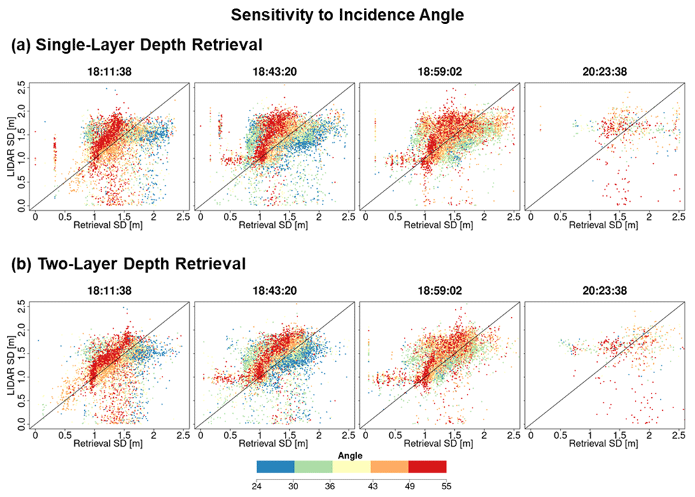
Figure A1The same as Fig. 7b but with pixels color coded according to the local SnowSAR incidence angle for all four flight lines and for one- (a) and two-layer (b) retrievals at 30 m resolution.
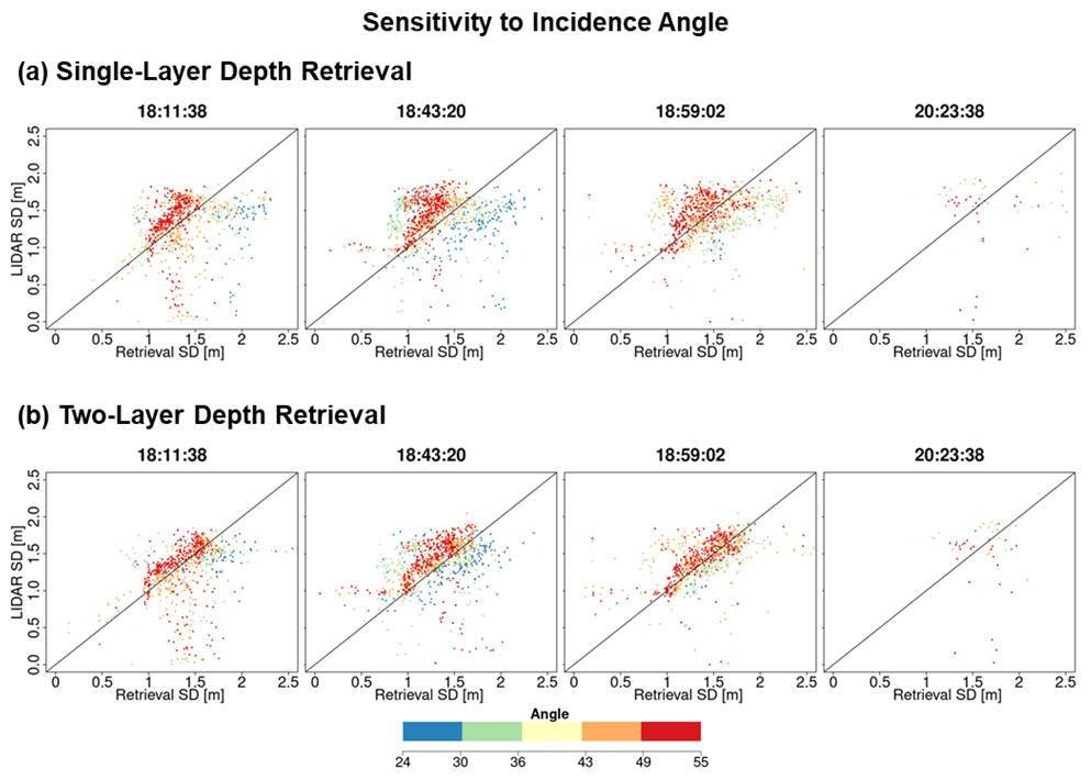
Figure A2The same as Fig. 7b but with pixels color coded according to the local SnowSAR incidence angle for all four flight lines and for one- (a) and two-layer (b) retrievals at 90 m resolution.
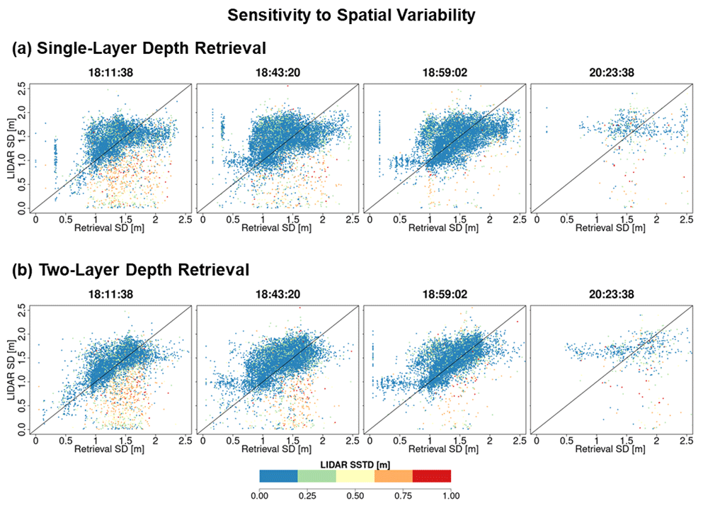
Figure A3Comparison between lidar snow depth (SD) and successful retrievals for one- and two-layer algorithms. The pixels are color coded according to the subgrid-scale variability of the 30 m upscaled lidar pixel.
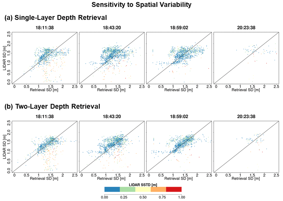
Figure A4Comparison between SnowSAR snow depth and successful retrievals. The pixels are color coded according to the subgrid-scale variability of the 90 m upscaled lidar pixel.
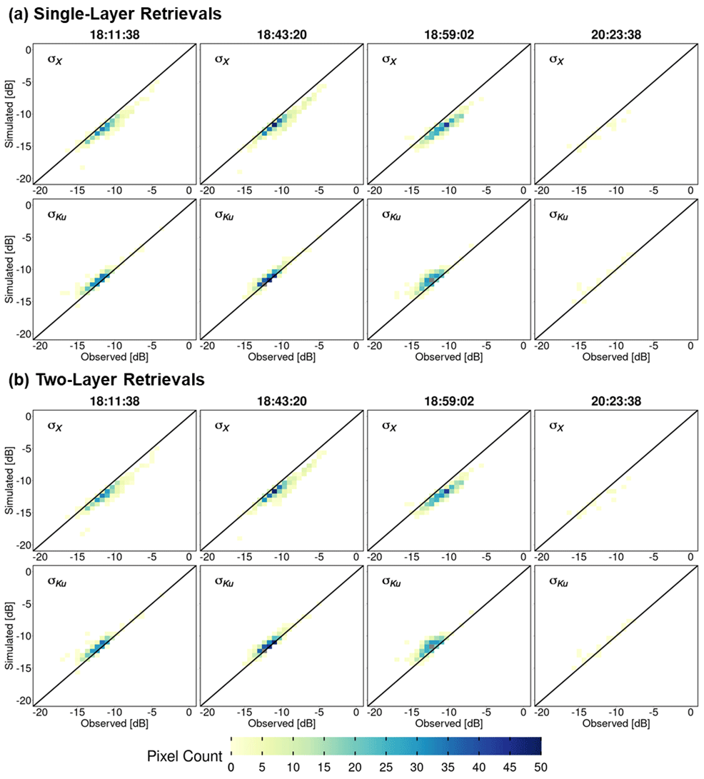
Figure A5Heatmaps of SnowSAR backscatter measurements (observed) versus retrievals (simulated) of backscatter at 90 m resolution: (a) one-layer snowpack and (b) two-layer snowpack for X (σX) and Ku (σKu) bands. Successful retrievals are for pixels with local incidence angles in the 30–45∘ range and relative residual backscatter (RRB) of less than 30 % for each of the four flights (see Table 4).

Figure A6Spatial distribution of successful SWE retrievals for one-layer (a) and two-layer (b) snowpacks in grassland pixels at 90 m resolution. Successful retrievals are for pixels with local incidence angles in the 30–45∘ range and relative residual backscatter (RRB) of less than 30 % for each of the four flights (see Table 4).
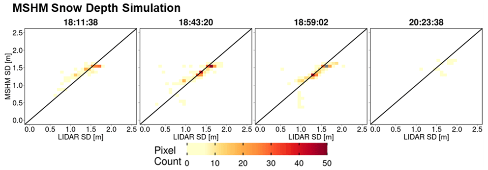
Figure A7Heatmaps of lidar snow depth and snow depth predicted by MSHM at the time of SnowSAR flights for overlapping pixels at 90 m resolution.
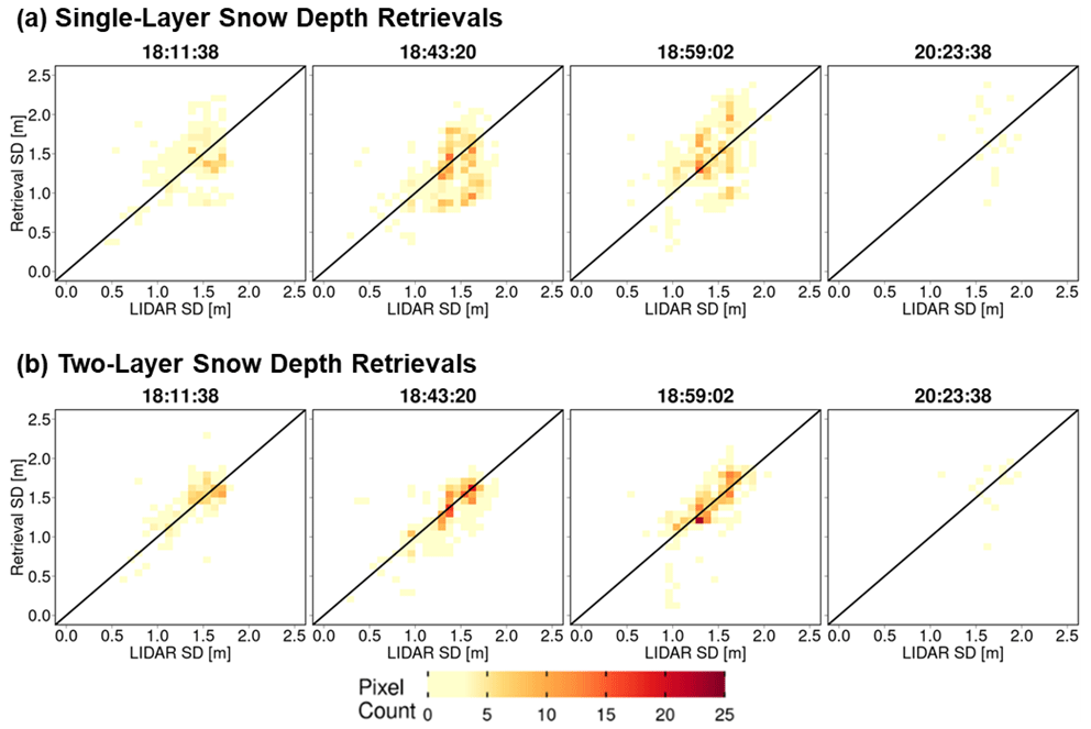
Figure A8Heatmaps of lidar versus successful snow depth (SD) retrievals at 90 m resolution using overlapping lidar and retrieval pixels. Successful retrievals are for pixels with local SnowSAR incidence angles in the 30–45∘ range and relative residual backscatter (RRB) of less than 30 % for each of the four flights (see Table 4). Lidar SD in pixels with subgrid-scale variability corresponding to standard deviation of less than 0.3 m for the upscaled 90 m lidar pixel are not included.
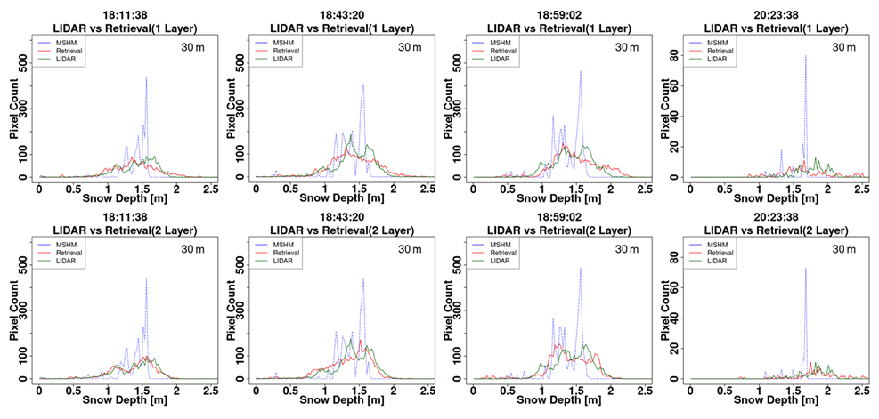
Figure A9Histogram of snow depth (SD) from lidar, MSHM, and successful retrievals at 30 m using one- and two-layer snowpacks. The total number of pixels for each snow depth product is the same. Successful retrievals are for pixels with local incidence angles in the 30–45∘ range and relative residual backscatter (RRB) of less than 30 % for each of the four flights (see Table 4). Lidar SD in pixels with subgrid-scale variability corresponding to standard deviation of less than 0.3 m for the upscaled 90 m lidar pixel are not included.
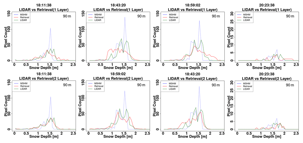
Figure A10Histogram of snow depth (SD) from lidar, MSHM, and successful retrievals at 90 m using one- and two-layer snowpacks. The total number of pixels for each snow depth product is the same. Successful retrievals are for pixels with local incidence angles in the 30–45∘ range and relative residual backscatter (RRB) of less than 30 % for each of the four flights (see Table 4). Lidar SD in pixels with subgrid-scale variability corresponding to standard deviation of less than 0.3 m for the upscaled 90 m lidar pixel are not included.
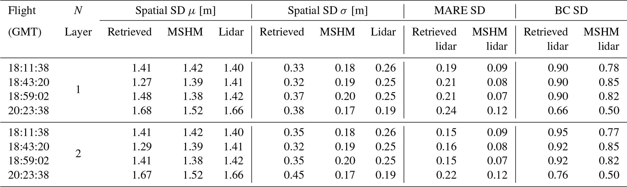
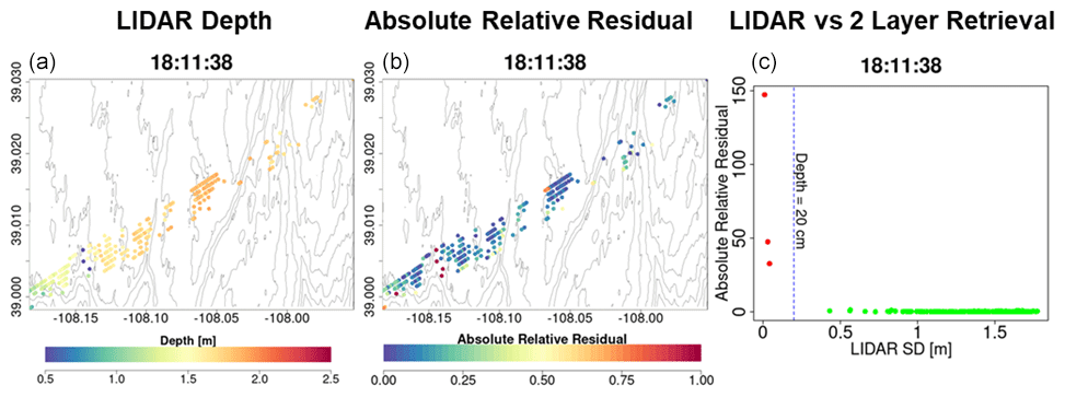
Figure A11Analysis of unsuccessful retrievals for pixels with large mean snow depth residuals at 90 m resolution. (a) Map of lidar snow depth highlighting in deep blue the locations where very shallow snow is attributed to measurement error. (b) Note the spatial agreement between shallow snow depth and very large residuals. (c) There are only a few points at the edges of forests and shallow snow depths that are flagged as not successful. The gray elevation contours are plotted every 50 m.
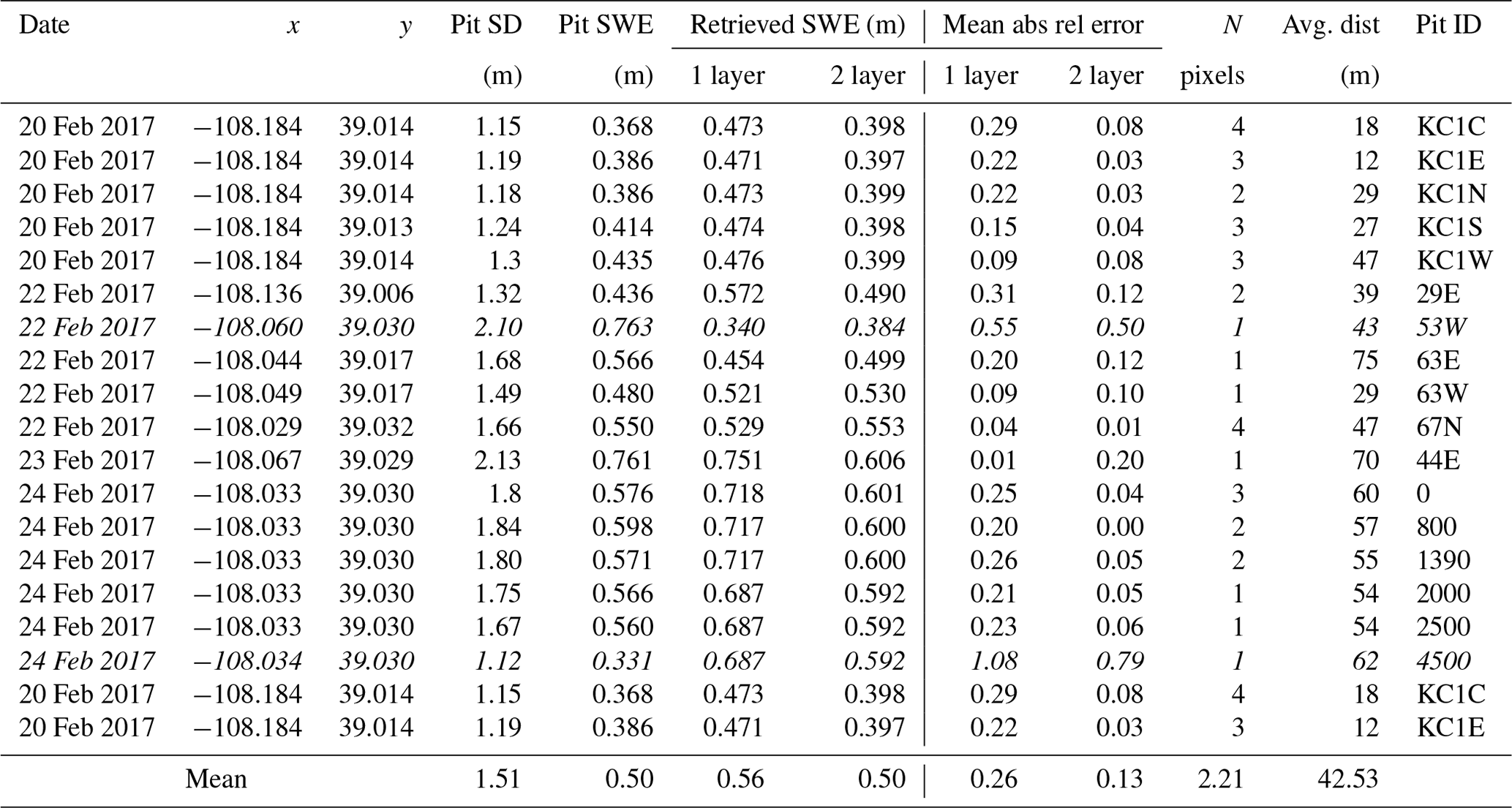
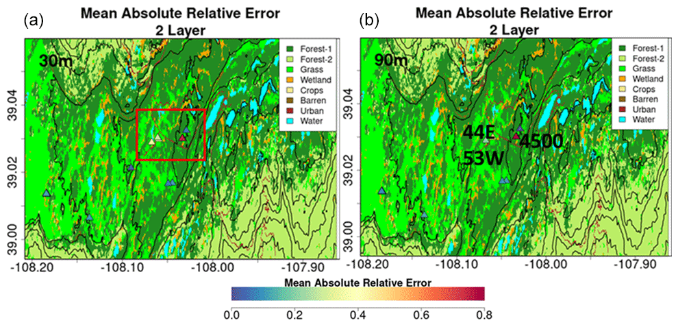
Figure A12Spatial context for snow pits with very large absolute relative errors (MARE) calculated as the mean of the relative difference between SWE retrievals within 100 m of the snow pit and the values at the snow pit. Locations with very large errors (orange to red) are inside the red box marked in the top plot. Snow pit 4500 is a region of complex land cover including evergreen forest, a road, and a pond. Snow pits 53W and 44E are close to each other on the same side of the road in expansive grassland.
Links to access all data sets used in this study are provided in Table 1.
APB and MD conceptualized the study. SS developed and implemented the retrieval framework, including modifications and coupling of the codes, under the guidance of APB. SS completed the retrievals and analyzed the results under the guidance of APB with input from MD. MD provided the original code of the Base-AM model. APB provided the original MSHM code. EK curated the SnowSAR data set. SS and APB wrote the paper and replied to reviewers with comments from MD and EK.
The contact author has declared that none of the authors has any competing interests.
Publisher's note: Copernicus Publications remains neutral with regard to jurisdictional claims made in the text, published maps, institutional affiliations, or any other geographical representation in this paper. While Copernicus Publications makes every effort to include appropriate place names, the final responsibility lies with the authors.
The authors acknowledge NASA's SnowEx field experiment program and the SnowEx community of investigators that made the data sets used in this work possible. The authors also wish to acknowledge prior model development and data analysis by Yueqian Cao, Jimin Pei, and Do-Hyuk Kang. Finally, the authors are grateful to the anonymous reviewers for their helpful comments and suggestions.
This research has been supported by the National Aeronautics and Space Administration (grant no. NNX17AL44G to Ana P. Barros and grant no. 80NSSC17K0200 to Michael Durand) and the National Oceanic and Atmospheric Administration Cooperative Institute for Research to Operations in Hydrology (CIROH) agreement (grant no. NA22NWS4320003 to Ana P. Barros).
This paper was edited by Alexandre Langlois and reviewed by two anonymous referees.
Baghdadi, N., Saba, E., Aubert, M., Zribi, M., and Baup, F.: Evaluation of Radar Backscattering Models IEM, Oh, and Dubois for SAR Data in X-Band Over Bare Soils, IEEE Geosci. Remote Sens. Lett., 8, 1160–1164, https://doi.org/10.1109/LGRS.2011.2158982, 2011.
Bateni, S. M., Margulis, S. A., Podest, E., and McDonald, K. C.: Characterizing Snowpack and the Freeze–Thaw State of Underlying Soil via Assimilation of Multifrequency Passive/Active Microwave Data: A Case Study (NASA CLPX 2003), IEEE T. Geosci. Remote, 53, 173–189, https://doi.org/10.1109/TGRS.2014.2320264, 2015.
Benjamin, S. G., Weygandt, S. S., Brown, J. M., Hu, M., Alexander, C. R., Smirnova, T. G., Olson, J. B., James, E. P., Dowell, D. C., Grell, G. A., Lin, H., Peckham, S. E., Smith, T. L., Moninger, W. R., Kenyon, J. S., and Manikin, G. S.: A North American Hourly Assimilation and Model Forecast Cycle: The Rapid Refresh, Mon. Weather Rev., 144, 1669–1694, https://doi.org/10.1175/MWR-D-15-0242.1, 2016.
Berliner, L. M.: Physical-statistical modeling in geophysics: Physical-Statistical Modeling in Geophysics, J. Geophys. Res.-Atmos., 108, 8776, https://doi.org/10.1029/2002JD002865, 2003.
Bhattacharyya, A.: On a Measure of Divergence between Two Multinomial Populations, Sankhya Ser. A., 7, 401–406, 1946.
Cao, Y. and Barros, A. P.: Weather-Dependent Nonlinear Microwave Behavior of Seasonal High-Elevation Snowpacks, Remote Sens., 12, 3422, https://doi.org/10.3390/rs12203422, 2020.
Cao, Y. and Barros, A. P.: Topographic controls on active microwave behavior of mountain snowpacks, Remote Sens. Environ., 284, 113373, https://doi.org/10.1016/j.rse.2022.113373, 2023a.
Cao, Y. and Barros, A. P.: Indirect Estimation of Vegetation Contribution to Microwave Backscatter Via Triple-Frequency SAR Data, in: IGARSS 2023 – 2023 IEEE International Geoscience and Remote Sensing Symposium, Pasadena, CA, USA, 3114–3117, https://doi.org/10.1109/IGARSS52108.2023.10281754, 2023b.
Deems, J. S., Painter, T. H., and Finnegan, D. C.: Lidar measurement of snow depth: a review, J. Glaciol., 59, 467–479, https://doi.org/10.3189/2013JoG12J154, 2013.
Dobson, M., Ulaby, F., Hallikainen, M., and El-rayes, M.: Microwave Dielectric Behavior of Wet Soil-Part II: Dielectric Mixing Models, IEEE T. Geosci. Remote, GE-23, 35–46, https://doi.org/10.1109/TGRS.1985.289498, 1985.
Durand, M. and Liu, D.: The need for prior information in characterizing snow water equivalent from microwave brightness temperatures, Remote Sens. Environ., 126, 248–257, https://doi.org/10.1016/j.rse.2011.10.015, 2012.
Hallikainen, M., Ulaby, F., Dobson, M., El-rayes, M., and Wu, L.: Microwave Dielectric Behavior of Wet Soil-Part 1: Empirical Models and Experimental Observations, IEEE T. Geosci. Remote, GE-23, 25–34, https://doi.org/10.1109/TGRS.1985.289497, 1985.
Huang, X. and Swain, D. L.: Climate change is increasing the risk of a California megaflood, Sci. Adv., 8, eabq0995, https://doi.org/10.1126/sciadv.abq0995, 2022.
Jacobs, J. M., Hunsaker, A. G., Sullivan, F. B., Palace, M., Burakowski, E. A., Herrick, C., and Cho, E.: Snow depth mapping with unpiloted aerial system lidar observations: a case study in Durham, New Hampshire, United States, The Cryosphere, 15, 1485–1500, https://doi.org/10.5194/tc-15-1485-2021, 2021.
Kang, D. H. and Barros, A. P.: Observing System Simulation of Snow Microwave Emissions Over Data Sparse Regions – Part I: Single Layer Physics, IEEE T. Geosci. Remote, 50, 1785–1805, https://doi.org/10.1109/TGRS.2011.2169073, 2012a.
Kang, D. H. and Barros, A. P.: Observing System Simulation of Snow Microwave Emissions Over Data Sparse Regions – Part II: Multilayer Physics, IEEE T. Geosci. Remote, 50, 1806–1820, https://doi.org/10.1109/TGRS.2011.2169074, 2012b.
Kim, E., Gatebe, C., Hall, D., Newlin, J., Misakonis, A., Elder, K., Marshall, H. P., Hiemstra, C., Brucker, L., De Marco, E., Crawford, C., Kang, D. H., and Entin, J.: NASA's snowex campaign: Observing seasonal snow in a forested environment, in: 2017 IEEE International Geoscience and Remote Sensing Symposium (IGARSS), 2017 IEEE International Geoscience and Remote Sensing Symposium (IGARSS), Fort Worth, TX, 1388–1390, https://doi.org/10.1109/IGARSS.2017.8127222, 2017.
Kim, R. S., Durand, M., Li, D., Baldo, E., Margulis, S. A., Dumont, M., and Morin, S.: Estimating alpine snow depth by combining multifrequency passive radiance observations with ensemble snowpack modeling, Remote Sens. Environ., 226, 1–15, https://doi.org/10.1016/j.rse.2019.03.016, 2019.
Lemmetyinen, J., Cohen, J., Kontu, A., Vehviläinen, J., Hannula, H.-R., Merkouriadi, I., Scheiblauer, S., Rott, H., Nagler, T., Ripper, E., Elder, K., Marshall, H.-P., Fromm, R., Adams, M., Derksen, C., King, J., Meta, A., Coccia, A., Rutter, N., Sandells, M., Macelloni, G., Santi, E., Leduc-Leballeur, M., Essery, R., Menard, C., and Kern, M.: Airborne SnowSAR data at X and Ku bands over boreal forest, alpine and tundra snow cover, Earth Syst. Sci. Data, 14, 3915–3945, https://doi.org/10.5194/essd-14-3915-2022, 2022.
Li, D., Durand, M., and Margulis, S. A.: Estimating snow water equivalent in a Sierra Nevada watershed via spaceborne radiance data assimilation, Water Resour. Res., 53, 647–671, https://doi.org/10.1002/2016WR018878, 2017.
Lowman, L. and Barros, A. P.: Investigating links between climate and orography in the central Andes: Coupling erosion and precipitation using a physical-statistical model, J. Geophys. Res.-Earth Surf., 119, 1322–1353, https://doi.org/10.1002/2013JF002940, 2014.
Macedo, K., Coccia, A., and Meta, A.: SnowEx17 SnowSAR Multi-look Synthetic Aperture Radar Backscatter Amplitude Images, Version 1, Boulder, Colorado USA, NASA National Snow and Ice Data Center Distributed Active Archive Center [data set], https://doi.org/10.5067/TWRTXCYBCBB8 (last access: 5 September 2023), 2020.
Manickam, S. and Barros, A.: Parsing Synthetic Aperture Radar Measurements of Snow in Complex Terrain: Scaling Behaviour and Sensitivity to Snow Wetness and Landcover, Remote Sens., 12, 483, https://doi.org/10.3390/rs12030483, 2020.
Martinec, J.: Areal modelling of snow water equivalent based on remote sensing techniques, in Snow, Hydrology and Forests in High Alpine Areas: Proceedings of the Vienna Symposium, IAHS Publ., 205, 121–129, 1991.
Mendoza, P. A., Musselman, K. N., Revuelto, J., Deems, J. S., López-Moreno, J. I., and McPhee, J.: Interannual and Seasonal Variability of Snow Depth Scaling Behavior in a Subalpine Catchment, Water Resour. Res., 56, e2020WR027343, https://doi.org/10.1029/2020WR027343, 2020.
Metropolis, N., Rosenbluth, A. W., Rosenbluth, M. N., Teller, A., and Teller, E.: Equation of State Calculations by Fast Computing Machines, J. Chem. Phys., 21, 1087–1092, https://doi.org/10.1063/1.1699114, 1953.
Mote, T. L., Grundstein, A. J., Leathers, D. J., and Robinson, D. A.: A comparison of modeled, remotely sensed, and measured snow water equivalent in the northern Great Plains: Comparison of Snow Water Equivalent, Water Resour. Res., 39, SWC41–SWC412, https://doi.org/10.1029/2002WR001782, 2003.
Musselman, K. N., Addor, N., Vano, J. A., and Molotch, N. P.: Winter melt trends portend widespread declines in snow water resources, Nat. Clim. Change, 11, 418–424, https://doi.org/10.1038/s41558-021-01014-9, 2021.
National Academies of Sciences, Engineering, and Medicine (NASEM): Thriving on Our Changing Planet: A Decadal Strategy for Earth Observation from Space, The National Academies Press, Washington, DC, https://doi.org/10.17226/24938, 2018.
Painter, T. H., Berisford, D. F., Boardman, J. W., Bormann, K. J., Deems, J. S., Gehrke, F., Hedrick, A., Joyce, M., Laidlaw, R., Marks, D., Mattmann, C., McGurk, B., Ramirez, P., Richardson, M., Skiles, S. M., Seidel, F. C., and Winstral, A.: The Airborne Snow Observatory: Fusion of scanning lidar, imaging spectrometer, and physically-based modeling for mapping snow water equivalent and snow albedo, Remote Sens. Environ., 184, 139–152, https://doi.org/10.1016/j.rse.2016.06.018, 2016.
Painter, T. H., Berisford, D. F., Boardman, J. W., Bormann, K. J., Deems, J. S., Gehrke, F., Joyce, M., Laidlaw, R., Mattmann, C., McGurk, B., Ramirez, P., Richardson, M., and Skiles, S. M.: ASO L4 Lidar Snow Depth 3m UTM Grid, Version 1, https://doi.org/10.5067/KIE9QNVG7HP0, 2018.
Pan, J., Durand, M. T., Vander Jagt, B. J., and Liu, D.: Application of a Markov Chain Monte Carlo algorithm for snow water equivalent retrieval from passive microwave measurements, Remote Sens. Environ., 192, 150–165, https://doi.org/10.1016/j.rse.2017.02.006, 2017.
Pan, J., Durand, M., Lemmetyinen, J., Liu, D., and Shi, J.: Snow water equivalent retrieved from X- and dual Ku-band scatterometer measurements at Sodankylä using the Markov Chain Monte Carlo method, The Cryosphere Discuss. [preprint], https://doi.org/10.5194/tc-2023-85, in review, 2023.
Proksch, M., Mätzler, C., Wiesmann, A., Lemmetyinen, J., Schwank, M., Löwe, H., and Schneebeli, M.: MEMLS3&a: Microwave Emission Model of Layered Snowpacks adapted to include backscattering, Geosci. Model Dev., 8, 2611–2626, https://doi.org/10.5194/gmd-8-2611-2015, 2015.
Rott, H., Cline, D. W., Duguay, C., Essery, R., Etchevers, P., Hajnsek, I., Kern, M., Macelloni, G., Malnes, E., Pulliainen, J., and Yueh, S. H.: CoReH2O, a dual frequency radar mission for snow and ice observations, in: 2012 IEEE International Geoscience and Remote Sensing Symposium, IGARSS 2012 – 2012 IEEE International Geoscience and Remote Sensing Symposium, Munich, Germany, 5550–5553, https://doi.org/10.1109/IGARSS.2012.6352348, 2012.
Sturm, M., Taras, B., Liston, G. E., Derksen, C., Jonas, T., and Lea, J.: Estimating Snow Water Equivalent Using Snow Depth Data and Climate Classes, J. Hydrometeorol., 11, 1380–1394, https://doi.org/10.1175/2010JHM1202.1, 2010.
Tsang, L., Durand, M., Derksen, C., Barros, A. P., Kang, D.-H., Lievens, H., Marshall, H.-P., Zhu, J., Johnson, J., King, J., Lemmetyinen, J., Sandells, M., Rutter, N., Siqueira, P., Nolin, A., Osmanoglu, B., Vuyovich, C., Kim, E., Taylor, D., Merkouriadi, I., Brucker, L., Navari, M., Dumont, M., Kelly, R., Kim, R. S., Liao, T.-H., Borah, F., and Xu, X.: Review article: Global monitoring of snow water equivalent using high-frequency radar remote sensing, The Cryosphere, 16, 3531–3573, https://doi.org/10.5194/tc-16-3531-2022, 2022.
Villano, M., Ustalli, N., Dell'Amore, L., Jeon, S.-Y., Krieger, G., Moreira, A., Peixoto, M. N., and Krecke, J.: NewSpace SAR: Disruptive Concepts for Cost-Effective Earth Observation Missions, in: 2020 IEEE Radar Conference (RadarConf20), 2020 IEEE Radar Conference (RadarConf20), Florence, Italy, 1–5, https://doi.org/10.1109/RadarConf2043947.2020.9266694, 2020.
Wiesmann, A. and Mätzler, C.: Microwave Emission Model of Layered Snowpacks, Remote Sens. Environ., 70, 307–316, https://doi.org/10.1016/S0034-4257(99)00046-2, 1999.