Evaporative controls on Antarctic precipitation: an ECHAM6 model study using innovative water tracer diagnostics

Improving our understanding of the controls on Antarctic precipitation is critical for gaining insights into past and future polar and global environmental changes. Here we develop innovative water tracing diagnostics in the atmospheric general circulation model ECHAM6. These tracers provide new detailed information on moisture source locations and properties of Antarctic precipitation. In the preindustrial simulation, annual mean Antarctic precipitation originating from the open ocean has a source latitude range of 49–35^∘ S, a source sea surface temperature range of 9.8–16.3 ^∘C, a source 2 m relative humidity range of 75.6 %–83.3 %, and a source 10 m wind velocity (vel10) range of 10.1 to 11.3 m s⁻¹. These results are consistent with estimates from existing literature. Central Antarctic precipitation is sourced from more equatorward (distant) sources via elevated transport pathways compared to coastal Antarctic precipitation. This has been attributed to a moist isentropic framework; i.e. poleward vapour transport tends to follow constant equivalent potential temperature. However, we find notable deviations from this tendency especially in the lower troposphere, likely due to radiative cooling. Heavy precipitation is sourced by longer-range moisture transport: it comes from 2.9^∘ (300 km, averaged over Antarctica) more equatorward (distant) sources compared to the rest of precipitation. Precipitation during negative phases of the Southern Annular Mode (SAM) also comes from more equatorward moisture sources (by 2.4^∘, averaged over Antarctica) compared to precipitation during positive SAM phases, likely due to amplified planetary waves during negative SAM phases. Moreover, source vel10 of annual mean precipitation is on average 2.1 m s⁻¹ higher than annual mean vel10 at moisture source locations from which the precipitation originates. This shows that the evaporation of moisture driving Antarctic precipitation occurs under windier conditions than average. We quantified this dynamic control of Southern Ocean surface wind on moisture availability for Antarctic precipitation. Overall, the innovative water tracing diagnostics enhance our understanding of the controlling factors of Antarctic precipitation.

1 Introduction

Antarctic climate is changing. The years 2022 and 2023 both witnessed new minima in sea ice extent and some of the largest extreme heat and melt events (Purich and Doddridge, 2023; Gorodetskaya et al., 2023). Increased moisture in Antarctic regions can directly drive warming: a range of model simulations show that increased poleward moisture transport in a warmer world is the largest contributor to Antarctic warming (Hahn et al., 2021). Furthermore, the warming ocean around Antarctica is very likely to lead to ice mass loss via sub-shelf melting and calving (DeConto and Pollard, 2016; DeConto et al., 2021). These Southern Ocean changes may impact local evaporation to drive Antarctic precipitation changes and therefore influence the Antarctic surface mass balance (Mottram et al., 2021; Lenaerts et al., 2019). It is possible that under a warmer future increases in Antarctic vapour and precipitation may contribute to changes in surface mass balance and extreme warming episodes (Davison et al., 2023; Medley and Thomas, 2018; Frieler et al., 2015; Winkelmann et al., 2012). Overall, projections of Antarctic contribution to future sea level rise due to these surface mass balance processes remain uncertain (IPCC, 2022).

Antarctic precipitation can manifest in various forms. It frequently falls as near-continuous clear-sky precipitation, so-called diamond dust (Bromwich, 1988). However, there are also relatively short-lived intrusions of maritime air, which can lead to episodes of heavier precipitation (Turner et al., 2019). Indeed, these events may contribute to 30 %–70 % of total precipitation across Antarctica, with likely more than 30 % of precipitation in the interior and up to 70 % in coastal regions (Turner et al., 2019). Whilst the mass balance of Antarctica can be estimated from satellite altimetry, gravimetry, and interferometry measurements (The IMBIE team, 2018), our understanding of thermodynamic and dynamic factors driving Antarctic precipitation remains limited.

Marine air intrusions are efficient at transporting moist and warm air from subtropics to Antarctica (Schlosser et al., 2010; Dittmann et al., 2016). The intrusions generally occur alongside strong meridional flow during planetary wave amplification (Adusumilli et al., 2021; Noone et al., 1999; Massom et al., 2004), sometimes in the form of atmospheric rivers (Gorodetskaya et al., 2014; Wille et al., 2021). Indeed, persistent ridges or dipolar patterns (with high pressure to the east and low to the west) are known to have contributed to heavy-precipitation events across a range of Antarctic sites, including EPICA Dome Concordia (EDC, Schlosser et al., 2016), Dome Fuji (Dittmann et al., 2016), and Dronning Maud Land (Gorodetskaya et al., 2014; Terpstra et al., 2021; Kurita et al., 2016; Noone et al., 1999). The marine air intrusions play a major role in heavy-precipitation events at both coastal locations and the Antarctic interior (Genthon et al., 1998; Gorodetskaya et al., 2014; Stohl and Sodemann, 2010).

Compared to heavy-precipitation events, light-precipitation events such as diamond dust seem to have received less attention. However, depending on the definitions used, light precipitation may contribute significantly to total precipitation over inland Antarctica (Stenni et al., 2016); and similar to heavy precipitation, light precipitation also depends on synoptic conditions (Schlosser et al., 2010). Developing an improved understanding of drivers of light precipitation is thus also important.

Variations in Antarctic precipitation have been linked to the principal modes of atmospheric circulation variability at southern mid-latitudes, particularly SAM and Pacific South American patterns associated with El Niño–Southern Oscillation (Marshall et al., 2017). The variations are associated with changes in zonal and meridional flows of atmospheric moisture around and towards Antarctica. While positive SAM polarity is linked to increased cyclogenesis and poleward storm track migration (Uotila et al., 2013; Fogt and Marshall, 2020), Antarctic regions do not show a uniform relationship between SAM and precipitation (Marshall et al., 2017; Medley and Thomas, 2018). To project Antarctic precipitation changes, it is important to understand how SAM impacts moisture transport paths.

Insights into Antarctic precipitation can be gleaned through its evaporative source regions and properties obtained from modelling studies. One of the widely applied tools for this is backward trajectory models (Sodemann and Stohl, 2009; Gimeno et al., 2010). Of backward trajectory studies, results regarding Antarctic precipitation sources from Sodemann and Stohl (2009) are probably more reliable than other Lagrangian studies with shorter (usually 5 d) backward trajectories (e.g. Gimeno et al., 2010). Based on a meteorological analysis dataset from October 1999 to April 2005, Sodemann and Stohl (2009) diagnosed moisture sources and sinks through changes in specific humidity along transport pathways of air parcels. While only ∼ 90 % of total precipitation can be attributed to specific sources with 20 d backward trajectories, annual moisture source latitudes of precipitation over the Antarctic Plateau were estimated to be 45 to 40^∘ S. Moisture source longitudes were generally located at 20 to 60^∘ to the west of precipitation locations. They also pointed out seasonal variations in moisture source latitudes of Antarctic precipitation, which are related to Antarctic topography, sea ice, baroclinicity, and mid-latitude land–sea distributions.

In addition to the Lagrangian trajectory approach, general circulation models (GCMs) can be equipped with water tracers to identify moisture sources. The water tracers track moisture that is evaporated from prescribed regions until it precipitates (e.g. Koster et al., 1986, 1992; Delaygue et al., 2000; Werner et al., 2001; Singh et al., 2016; Wang et al., 2020). Typically, the globe is divided into multiple source regions, and then the contribution of each region to total precipitation at any location can be quantified. This Eulerian method is complementary to the Lagrangian one and offers an elegant online diagnostic of moisture sources. For example, Koster et al. (1992) divided the globe into multiple regions based on climatological sea surface temperature (SST) bins, and they approximated moisture source SST of precipitation from each prescribed region as the middle value of the bin. Then mass-weighted average moisture source SST of Antarctic July precipitation was estimated to be around 11.6 ^∘C.

Recently, Fiorella et al. (2021) introduced a new approach to using water tracers in GCMs. Their process-oriented water tracers can track moisture properties related to evaporation, transport, and condensation. This approach is more computationally efficient than the previous approach of tagging moisture from individual prescribed regions, and it prevents bias while estimating evaporative source properties (see Sect. 2.2.1 for details). Here, we employ and further develop this approach to quantify moisture source regions, locations, and properties of Antarctic precipitation in preindustrial climate.

The paper is organised as follows: Fig. 2 introduces the materials and methods, and Fig. 3 presents the results; conclusions and perspectives are given in Fig. 4.

2 Materials and methods

2.1 Model and simulation

For this study, we use the ECHAM6 atmospheric GCM, which was developed by the Max Planck Institute for Meteorology (MPI-M) in Hamburg (Stevens et al., 2013). In ECHAM6, the primitive equations are formulated in a mixed finite-difference and spectral discretisation with a semi-implicit time scheme. The dynamical part is represented by truncated series of spherical harmonics in the horizontal and a finite-difference scheme in the vertical. Moisture transport is treated using a mass-conserving flux form semi-Lagrangian algorithm on a Gaussian grid. The vertical coordinate consists of a hybrid sigma-pressure coordinate system, which is terrain-following at lower levels and flattens to surfaces of constant pressure at upper levels. We use a T63L47 resolution, i.e. a resolution equivalent to 1.87^∘ × 1.87^∘ horizontal grid size and 47 vertical levels extending to 0.01 hPa. This resolution captures the overall shape of the Antarctic ice sheet with the caveat that complex coastal topography is not captured well (Fig. B1).

We set up a preindustrial condition simulation using sea surface temperature (SST) and sea ice concentration (SIC) data from the Atmospheric Modelling Intercomparison Project (AMIP, Fig. B2a and b). These are climatological monthly mean data from 1870 to 1899 (Durack et al., 2022). For sea-ice-covered areas, SST is set to −1.8 ^∘C. We run the simulation for 60 years and use the last 50 years in the analysis. Daily ECHAM6 model output is used for the analyses.

The formulation of air–sea moisture fluxes in the model is relevant for moisture source properties. In ECHAM6, oceanic evaporation is estimated based on bulk parameterisation (Hoffmann et al., 1998; Liu et al., 1979; Yu and Weller, 2007):

$$\begin{array}{}\text{(1)}& E=\mathit{\rho }{C}_{\mathrm{e}}\left|V\right|(q_{\mathrm{s}}-q),\end{array}$$

where E represents evaporation, ρ the air density, C_e the turbulent exchange coefficient related to atmospheric stability (Fairall et al., 2003), $\left|V\right|$ the wind speed at the lowest model level, q_s the saturation specific humidity at the surface temperature, and q the specific humidity at the lowest model level.

2.2 Water tracing methods

Previous versions of ECHAM had both water isotopes and standard water tracers incorporated (Hoffmann et al., 1998; Werner et al., 2001). However, the latest version of ECHAM, ECHAM6, has so far only been equipped with water isotope tracers (Cauquoin et al., 2019). Building upon the model code infrastructure of water isotopes, for this work we implemented two types of water tracers: (a) standard water tracers, which are usually applied to track water evaporating from prescribed regions; and (b) scaled-flux water tracers, which follow the concepts of Fiorella et al. (2021) and were referred to as process-oriented tracers in their paper. These two tracer sets are used together here in a new and complementary approach.

For the standard water tracers (hereafter “prescribed-region” tracers), we prescribe seven complementary regions. These are the open ocean south of 50^∘ S; Southern Hemisphere (SH) sea ice; Pacific, Indian, and Atlantic oceans north of 50^∘ S; the Antarctic ice sheet (AIS); and land exclusive of AIS. As sea ice changes at each time step, the prescribed SH sea ice region follows the changes. This is in itself a new form of dynamic prescribed-region water tracing. Where a grid cell contains both open ocean and sea ice, we track these sub-grid-scale fluxes separately.

The implementation of scaled-flux water tracers follows Fiorella et al. (2021), with some modifications for ECHAM6 as described in Appendix A. For example, we only trace moisture evaporated from the open ocean, and we use three water tracers for each source property to ensure the conservation of water masses and limit the propagation of numerical errors. The scaled-flux tracing method can be used to tag any property associated with evaporation. Given recent interests in how the changing Southern Ocean will affect Antarctic precipitation, we focus here on properties which are most closely associated with evaporation. Based on Eq. (1), in ECHAM6 $\left|V\right|$ is approximated as 10 m wind velocity (vel10); q_s depends on SST; and q is approximated as 2 m specific humidity, which is linked to 2 m relative humidity (rh2m) and associated air temperature (Yu and Weller, 2007). So, we chose to trace source longitude, latitude, SST, rh2m, and vel10. Please see Fig. A for a fuller description of how the scaled-flux water tracers are implemented in ECHAM6.

Based on the source latitude and longitude of precipitation and precipitation site location, a source–sink distance can be estimated by calculating the geographical distance from moisture source to precipitation site assuming a spherical earth surface. Note that this geographical distance is smaller than the actual transport distance of the moisture. Nevertheless, this source–sink distance is physically meaningful and is likely very closely associated with the actual modelled moisture transport distance.

2.2.1 Evaluating the scaled-flux water tracing method

To evaluate the performance of the scaled-flux water tracing method, we compare it with results from the prescribed-region water tracing method.

Prescribed-region water tracers can also be used to estimate evaporation source properties (Koster et al., 1992; Delaygue et al., 2000; see Fig. 1). As an example, we divide the global open ocean into multiple regions based on 10^∘ latitude bins. We assume source latitude of precipitation from each region as the middle value of the bin (e.g. 5^∘ for the latitude bin 0–10^∘). Then we estimate mass-weighted mean source latitude of precipitation from all regions (Fig. 1b). The results are close to those from scaled-flux water tracers (Fig. 1a): the maximum absolute difference between the two estimates is less than 2.8^∘, and the mean absolute difference is 0.6^∘ (Fig. 1c). Comparisons of source longitude, SST, rh2m, and vel10 from the two approaches show similar results.

The comparison provides some insights regarding properties of the two water tracing approaches. Firstly, since two different methods provide comparable estimates, we are confident that the tracers correctly reflect moisture sources in ECHAM6. Secondly, the scaled-flux water tracing method is more computationally efficient than the prescribed-region water tracing method. Figure 1a is obtained with three water tracers, whereas Fig. 1b is obtained with 18 water tracers, where each water tracer needs ∼ 10 % additional computational time. Thirdly, the scaled-flux water tracing method is more precise than the prescribed-region water tracing method. The colour strips in Fig. 1c with alternating signs in each 10^∘ bin are bias associated with prescribed-region water tracers. The bias results from the approximation of moisture source latitude from each region as the middle value of the bin. It can be reduced by decreasing bin intervals (not shown), which demands even more water tracers and more computational resources. In the study of Koster et al. (1992), temporal variations of SST might lead to even larger bias. While the prescribed-region water tracers can provide information regarding contributions of each prescribed region and thus the distribution of moisture sources, the scaled-flux water tracing method can only obtain mass-weighted mean moisture source locations and properties. In addition, compared to Lagrangian trajectory diagnostics, the Eulerian water tracing methods cannot infer transport pathways of moisture.

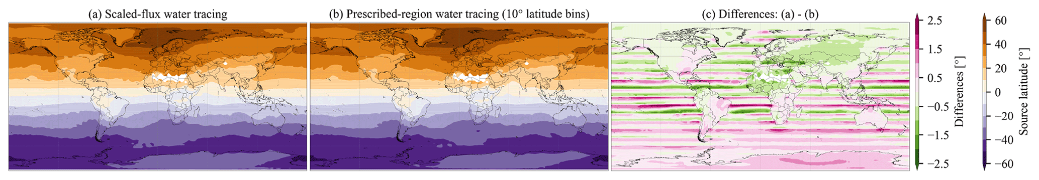
Figure 1 Mass-weighted mean open-ocean evaporative source latitude of annual mean precipitation estimated from (a) the scaled-flux water tracing approach and (b) the prescribed-region water tracing approach using 10^∘ latitude bins. (c) The differences between panel (a) and (b). We utilised only 1-year simulation data here with a 1-year spin-up period to save computational resources. Positive source latitude difference means more northward.

2.3 Defining heavy and light precipitation

To define heavy and light precipitation, we firstly need to define a “precipitation day”. Turner et al. (2019) defined a precipitation day in Antarctica as having more than 0.02 mm d⁻¹ precipitation. However, a threshold of 0.02 mm d⁻¹ excludes low daily precipitation amounts that can contribute to more than 10 % of total precipitation amount over the Antarctic interior in both the ERA5 reanalysis (Hersbach et al., 2020) and the simulation. We therefore use a lower threshold of 0.002 mm d⁻¹. This ensures we account for more than 99.7 % of the total Antarctic precipitation amount. We note that this definition has limited transferability to station observations.

We define light precipitation as that which cumulatively contributes to 10 % of total precipitation, while all other precipitation days have higher precipitation rates. For the definition of heavy precipitation, we follow the Turner et al. (2019) definition and use the top 10 % precipitation days. Note the definition of light precipitation, based on precipitation amount, is different from that of heavy precipitation, based on precipitation rates. This is because a definition of light precipitation as the 10 % lowest precipitation days would contribute to less than 0.3 % of total Antarctic precipitation and less than 1.1 % of total precipitation at individual grid boxes.

2.4 The Southern Annular Mode (SAM) index

We calculate monthly SAM values as the difference in normalised zonal mean sea level pressure at 40 and 65^∘ S (Gong and Wang, 1999). We define SAM+ and SAM− months as months with SAM values deviating more than 1 standard deviation from the mean (calculated from the 50-year period) in the positive and negative directions, respectively.

3 Results

3.1 The simulation of Antarctic precipitation and the SAM

The overall spatial patterns of accumulation are captured in the ECHAM6 model results (Fig. 2a vs. 2b). The simulated accumulation is lower than the Medley and Thomas (2018) reconstruction over the Antarctic Plateau and the Antarctic Peninsula (AP) and is higher than the reconstruction across some coastal areas (Fig. 2c). The relatively coarse (T63) spatial resolution of the simulation might not be adequate to simulate coastal precipitation. Furthermore, the reconstruction of Antarctic accumulation might be affected by limited ice core records and local processes such as melt events in coastal regions (Monaghan et al., 2006). Interannual variability, measured as the percentage of annual standard deviation to the annual mean, is slightly higher in the ECHAM6 simulation (∼ 20 %) than in the Medley and Thomas (2018) dataset (∼ 10 %, Fig. 2a vs. 2b).

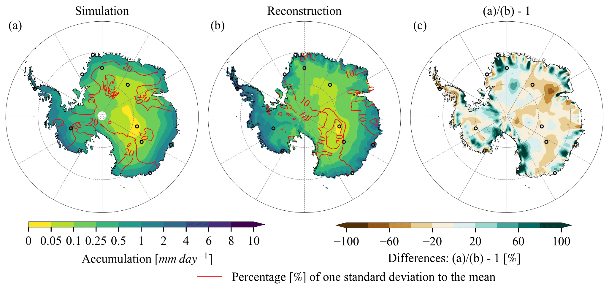
Figure 2 Annual mean accumulation rate over Antarctica in (a) the preindustrial simulation and (b) the reconstruction of Medley and Thomas (2018) for the period 1800–1900. The Medley and Thomas (2018) dataset is based on combining ice core data with spatial patterns of accumulation derived from the MERRA-2 reanalysis (Gelaro et al., 2017). (c) Differences as a percentage of the Medley and Thomas (2018) reconstruction. For the comparison, both datasets are regridded to $\mathrm{1}{}^{\circ }\times \mathrm{1}{}^{\circ }$ grids using a bilinear method. Accumulation in the simulation is defined as differences between precipitation and evaporation, while post-depositional effects are not considered. Black empty circles represent 10 sites whose names are given in Fig. B1b.

The annual cycle of Antarctic precipitation in the simulation is similar to ERA5 (Fig. B3), with precipitation averaged over Antarctica exceeding 15 mm per month from March to August, a peak in May, and a minimum in December–January. Spatial patterns of heavy-precipitation contributions to total precipitation in the simulation are likewise very similar to those in Turner et al. (2019), with high values around major ice shelves (not shown).

We evaluated the modelled SAM index against the SAM index based on station observations between 1971–2000 (Marshall, 2003). Due to the SAM definition, both datasets have similar mean values and standard deviations. We therefore look at monthly zonal mean sea level pressure (MSLP) at 40 and 65^∘ S to check whether the simulation features realistic pressure fields (Fig. B4). Simulation results deviate less than 1 standard deviation from ERA5 for both MSLP at 40 and 65^∘ S (Fig. B4a) and for their differences (Fig. B4b). Root mean squared errors between simulated and assimilated MSLP at 40 and 65^∘ S, as well as their differences, are 1.0, 1.4, and 1.5 hPa, respectively.

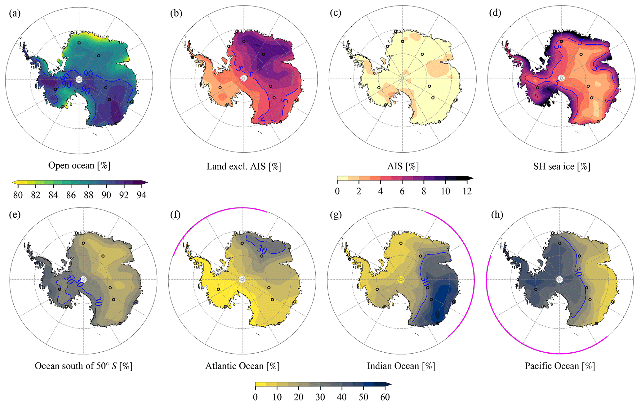
Figure 3 Relative contributions of prescribed regions to annual mean precipitation across Antarctica. The prescribed regions include (a) the open ocean, (b) land exclusive of AIS, (c) AIS, (d) SH sea ice, (e) the open ocean south of 50^∘ S, (f) Atlantic Ocean, (g) Indian Ocean, and (h) Pacific Ocean north of 50^∘ S. Relative contributions from the open ocean (a) are the sum of panels (e)–(h). Magenta lines in panels (f)–(h) represent the Atlantic, Indian, and Pacific Ocean sectors, respectively. Blues lines in each figure are contours of relative contributions. Moisture source region information is derived from the prescribed-region water tracers.

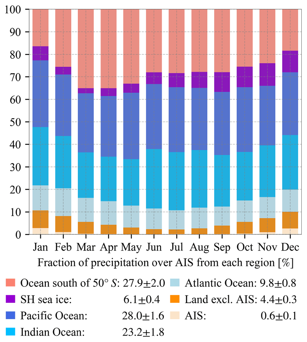
Figure 4 Relative contributions of seven prescribed regions to monthly mean precipitation integrated over Antarctica. The contributions (±1 standard deviation) to annual mean precipitation over Antarctica are given in the legend. Moisture source region information is derived from the prescribed-region water tracers.

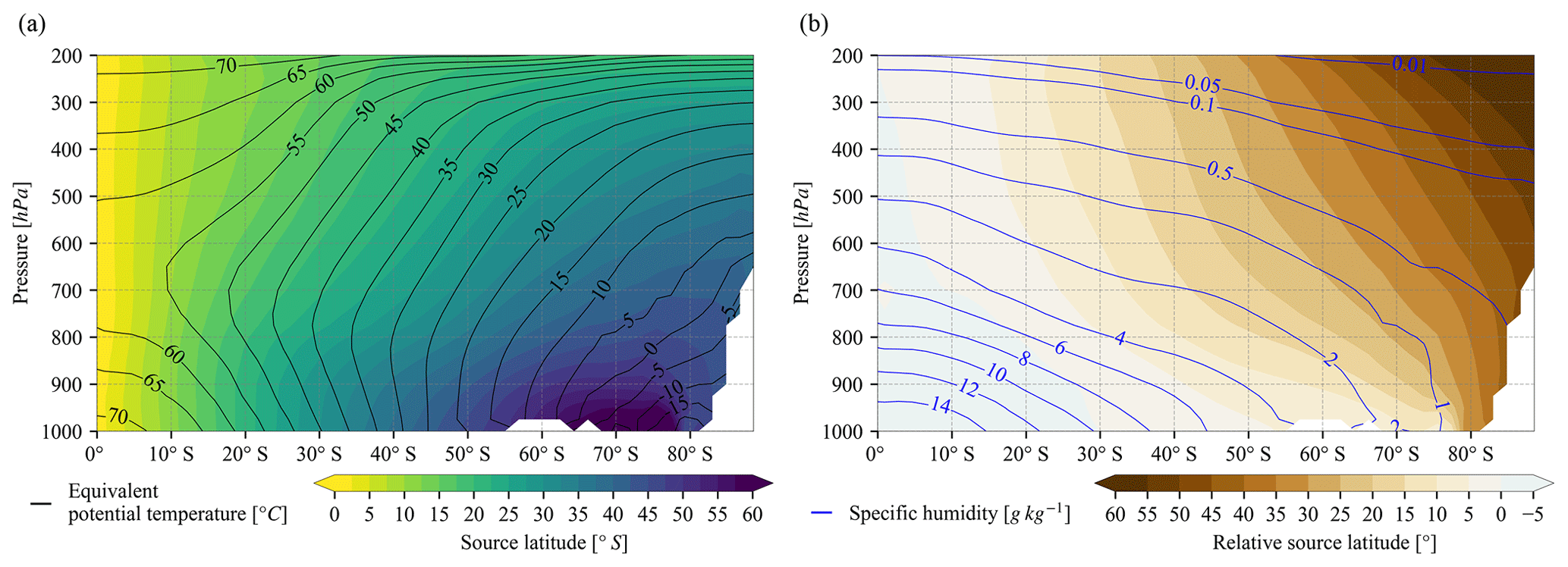
Figure 5 Zonal-averaged mass-weighted mean open-ocean (a) evaporative source latitude and (b) relative source latitude of annual mean atmospheric humidity originating from the open ocean. Black contours in panel (a) show the zonal mean annual mean equivalent potential temperature at an interval of 5 ^∘C. Blue contours in panel (b) show zonal mean annual mean atmospheric specific humidity at values of [0.01, 0.05, 0.1, 0.5, 1, 2, 4, 6, 8, 10, 12, 14] g kg⁻¹. Relative source latitude is defined as differences between source latitude and local latitude. Positive source latitude difference means more equatorward. Moisture source latitude information is derived from the scaled-flux water tracers.

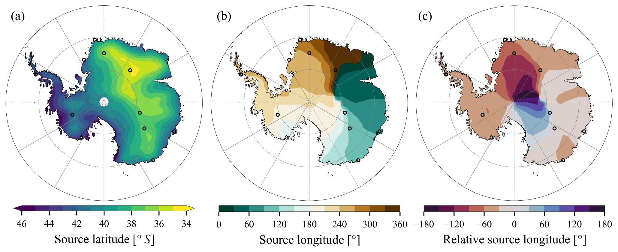
Figure 6 Mass-weighted mean open-ocean (a) evaporative source latitude, (b) evaporative source longitude, and (c) relative source longitude of annual mean precipitation. Relative source longitude is estimated as differences between source longitude and local longitude. Positive source longitude difference means more eastward. Moisture source location information is derived from the scaled-flux water tracers.

3.2 Moisture source regions and locations of Antarctic precipitation

Prescribed-region water tracers are used here to infer moisture source region information. We find that 89 % of modelled annual mean Antarctic precipitation comes from oceanic evaporation (Figs. 3a and 4), which is obtained by summing up contributions from all ocean basins. Less than 1 % of the precipitation is sourced from continental sublimation over Antarctica (Figs. 3c and 4). The continental recycling occurs mainly around major ice shelves in December and January (up to 3 %) with the most intense solar insolation. The magnitude of continental recycling depends on the parameterisation of surface sublimation fluxes (Gerber et al., 2023) and thus requires further investigation, e.g. intermodel comparisons or sensitivity tests of surface schemes. Antarctic precipitation sourced from other land masses is higher (by ∼ 4 %) than that from Antarctica itself (Figs. 3b and 4). Similar to the CESM1 simulation of Wang et al. (2020), in the ECHAM6 simulation most of the non-Antarctica land-sourced precipitation arrives in austral summer (contributing to 8 % of summer precipitation, compared to only 2 % of winter precipitation). Moisture originating from these other land masses has a relatively larger contribution to the East AIS (EAIS) precipitation (5.6 %), compared to the West AIS (WAIS, 2.6 %) and AP (2.7 %). The remaining Antarctic precipitation (6.1 %) is sourced from SH sea ice areas (Figs. 3d and 4). This surface type has notably larger contributions in coastal regions. Precipitation sourced from sea ice reaches its maximum between September and December (∼ 10 %), due to combined influences of a relatively large sea ice area and increased solar insolation.

Regarding precipitation sourced from the open ocean, 28 % of this precipitation comes from the open ocean south of 50^∘ S (Figs. 3e and 4). This region contributes a larger proportion of precipitation over WAIS (35 %) and AP (36 %) compared to EAIS (23 %). Contributions from both the Indian Ocean (23 %) and the Pacific Ocean (28 %) are 2 to 3 times that from the Atlantic Ocean (10 %) north of 50^∘ S (Fig. 4). This is at least partly attributable to the sizes of these ocean basins: between the Equator and 50^∘ S, areas of the Indian and Pacific oceans are 1.4 and 2.3 times that of the Atlantic Ocean, respectively. The three ocean basins contribute relatively more precipitation within their corresponding Antarctic sectors, though with a tendency to an eastward shift (∼ 30–60^∘) due to the predominant eastward transport of water vapour around Antarctica (Fig. 3f–h).

Water vapour has to rise to higher altitudes to reach central Antarctica (Noone and Simmonds, 2002; Stohl and Sodemann, 2010; Wang et al., 2020; Terpstra et al., 2021). As a result, the higher, remote central regions of Antarctica tend to receive moisture sourced from more equatorward regions. Moisture sourced from more poleward regions, e.g. ocean south of 50^∘ S and SH sea ice compared to land exclusive of AIS, is transported at lower altitudes to Antarctica; therefore, its precipitation contributions are larger over WAIS and AP with lower elevations than EAIS (Fig. 3b, d, and e). This pattern has been attributed to a moist isentropic framework (Pauluis et al., 2010; Bailey et al., 2019; Wang et al., 2020), which suggests that poleward moisture transport approximates a moist adiabatic poleward ascent, i.e. following contours of equivalent potential temperature. While it is a useful framework to conceptualise the broad scope of the atmospheric moisture transport, we find notable deviations from this framework in Fig. 5. The moisture transport pathways intersect moist isentropes in the lower troposphere, which might be expected due to radiative cooling effects of water vapour (Manabe and Strickler, 1964).

Elevated transport pathways to central Antarctic regions also impact mass-weighted mean open-ocean evaporative source latitude (source latitude thereafter). Source latitude of annual mean precipitation ranges from 49 to 35^∘ S across Antarctica and averages to 41^∘ S over all of Antarctica (Fig. 6a). These values are close to the estimate from Sodemann and Stohl (2009) of 45 to 40^∘ S across the Antarctic Plateau, though their study was for present-day climate rather than preindustrial climate as in this study. The elevated transport pathways mean that source latitude of EAIS precipitation is more equatorward by ∼ 3^∘ compared to that of WAIS and AP (40^∘ S vs. 43^∘ S). Also, Antarctic precipitation at surface elevations above 2250 m comes from more equatorward regions by 4^∘ compared to precipitation occurring below 2250 m (38^∘ S vs. 42^∘ S).

Regarding seasonality, source latitudes are most equatorward in December–January–February (DJF) and most poleward in March–April–May (MAM) and June–July–August (JJA) (Fig. B5a; an average 3.3^∘ DJF to JJA shift over Antarctica). This cannot be explained through Antarctic sea ice extent, as the minimal sea ice extent during austral summer DJF is favourable for more evaporation from polar oceans. We propose that weaker westerlies in DJF compared to JJA, induced by smaller meridional thermal gradients, may promote equatorward shifted moisture sources (see Sect. 3.5 for details).

Antarctic precipitation generally comes from the west (Fig. 6b–c), except for precipitation in a sector between the South Pole and EDC which appears to originate from the east. This pattern is also observed in the results of Sodemann and Stohl (2009) for DJF precipitation (see their Fig. 2c). We speculate that this might be from the far west, with a rotation of more than 180^∘, probably under impacts of the Amundsen Sea Low. This would need to be investigated through Lagrangian moisture trajectory diagnostics. Source longitude over Antarctica displays the largest inter-annual variability of all source properties (Fig. B5b).

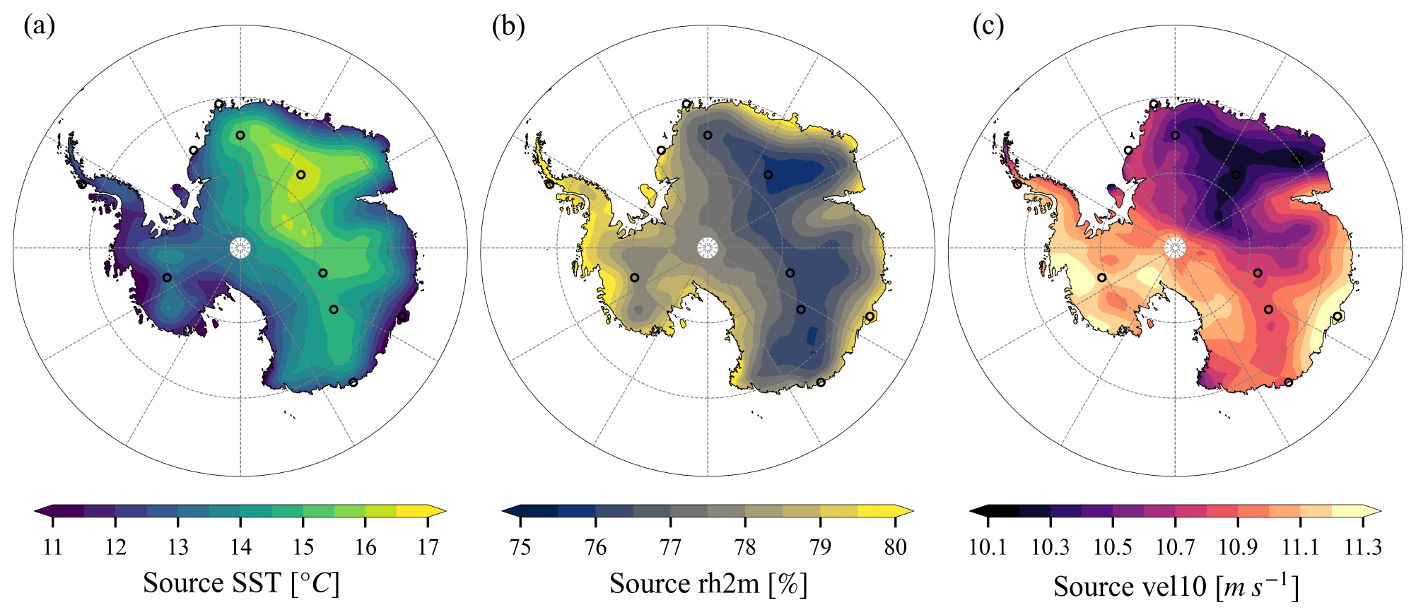
Figure 7 Mass-weighted mean open-ocean evaporative (a) source SST, (b) source rh2m, and (c) source vel10 of annual mean precipitation. Moisture source property information is derived from the scaled-flux water tracers.

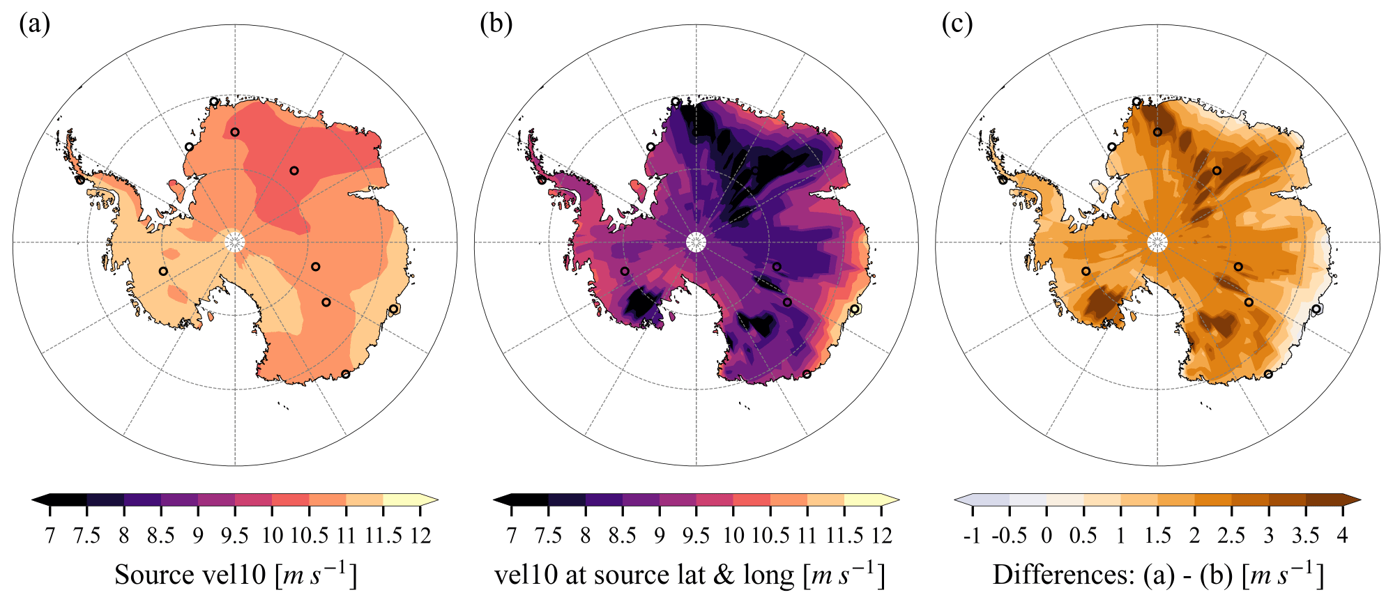
Figure 8 (a) Mass-weighted mean open-ocean evaporative source vel10 of annual mean precipitation. (b) Annual mean vel10 at source locations of annual mean precipitation. (c) Differences between panel (a) and (b). The average difference over Antarctica is ∼ 2.1 m s⁻¹.

3.3 Moisture source properties of Antarctic precipitation

After studying moisture source regions and locations, we now consider other oceanic source properties which control evaporation: vel10, rh2m, and SST.

Source SST of annual mean precipitation varies between 9.8 and 16.3 ^∘C across Antarctica, averaging to 12.8 ^∘C (Fig. 7a). This lies within the range of estimates from the literature: 15–22 ^∘C by Petit et al. (1991), 9–14 ^∘C by Koster et al. (1992), and 10–12 ^∘C by Delaygue et al. (2000). Analogous to source latitude, EAIS precipitation originates from ∼ 1 ^∘C warmer oceans compared to WAIS and AP (13.3 vs. 12.1 and 12.4 ^∘C), and Antarctic regions at altitudes higher than 2250 m receive precipitation from 2 ^∘C warmer oceans compared to lower regions (14.5 vs. 12.5 ^∘C). Source rh2m of annual mean precipitation ranges from 75.6 % to 83.3 % across Antarctica and averages to 78.3 % (Fig. 7b). Again, EAIS derives its precipitation from oceans with lower rh2m than WAIS and AP by 1 % and 1.5 %, respectively (77.9 % vs. 78.9 % and 79.4 %), and Antarctic regions above 2250 m elevations obtain precipitation from oceans with lower rh2m by 1.7 % compared to lower regions (76.9 % vs. 78.6 %). Interestingly, source vel10 of annual mean precipitation has a very narrow range over Antarctica of just 10.1 to 11.3 m s⁻¹, with 11 m s⁻¹ on average (Fig. 7c). Source vel10 of EAIS precipitation (10.8 m s⁻¹) is only marginally lower than that of WAIS (11.2 m s⁻¹) and AP (10.9 m s⁻¹), and the difference is also small for regions above and below 2250 m (10.7 vs. 11 m s⁻¹). Further studies are merited to investigate the relationship between this narrow band of source vel10 of annual mean precipitation over Antarctica and extratropical cyclones propagating along the Southern Ocean storm tracks (Aemisegger and Papritz, 2018; Sinclair and Dacre, 2019).

Moisture source locations and properties can be affected by different factors. As evaporation occurs preferentially during higher wind speeds at an oceanic grid cell (Eq. 1), moisture source vel10, which is weighted by evaporation fluxes, is larger than mean vel10 at this grid cell. Indeed, differences between moisture source vel10 and climatological vel10 at moisture source locations of annual mean precipitation are generally positive, with an Antarctic average value of 2.1 m s⁻¹ (Fig. 8). There are seasonal variations in the impact of source vel10: Antarctic mean differences are +2.9 m s⁻¹ in DJF, +1.6 m s⁻¹ in MAM, +1.3 m s⁻¹ in JJA, and +2.2 m s⁻¹ in September–October–November (SON). The consistent 1–3 m s⁻¹ offset in all seasons suggests that Southern Ocean surface wind exerts a dynamic control on moisture availability for Antarctic precipitation. Annual cycles of source latitude and properties are controlled by meridional thermal gradients, sea ice variations, and seasonal climate variations at mid-latitudes. For example, precipitation is from more southern oceans in MAM because of less sea ice than in JJA (Fig. B5a3 vs. a4), precipitation is from warmer oceans in MAM due to higher SST at mid-latitudes than in JJA (Fig. B5d3 vs. d4), and precipitation is from less windy regions in DJF due to weaker meridional thermal gradients and weaker westerlies than in JJA (Fig. B5f2 vs. f4).

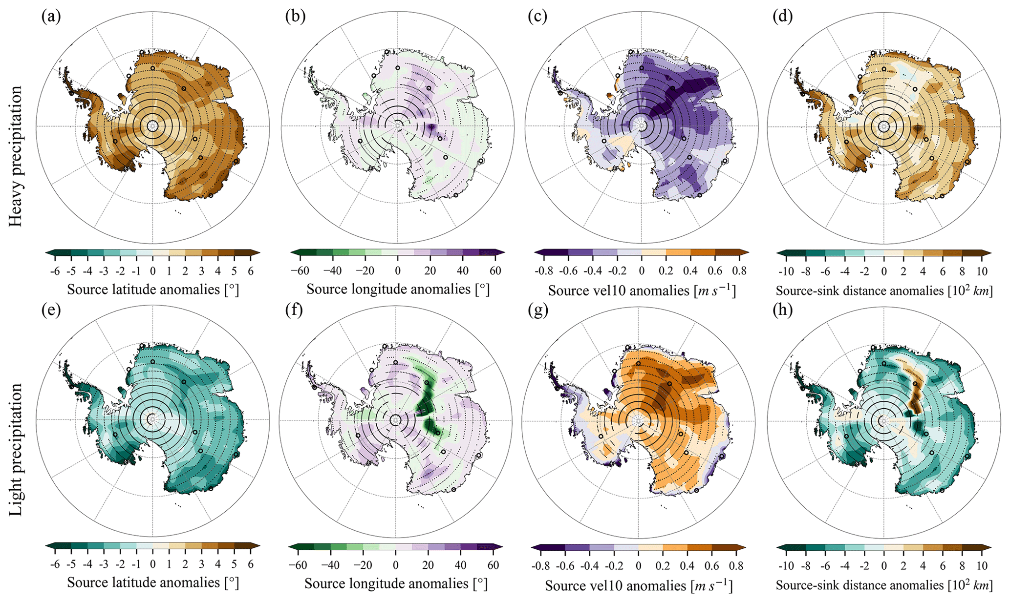
Figure 9 Moisture source anomalies of (a–d) heavy precipitation and (e–h) light precipitation. Heavy-precipitation and light-precipitation source anomalies are relative to non-heavy-precipitation and non-light-precipitation days, respectively. Source properties include mass-weighted mean open-ocean evaporative (a, e) source latitude, (b, f) source longitude, (c, g) source vel10, and (d, h) source–sink distance. Stippling points represent significant differences at the 5 % significance level based on statistical tests: for all variables except source longitude, Student's t test with the Benjamini–Hochberg procedure controlling false discovery rates (Benjamini and Hochberg, 1995) is adopted; for source longitude, the Watson–Williams F test for circular statistics (Watson and Williams, 1956) is employed. Positive source latitude difference means more equatorward, and positive source longitude difference means more eastward.

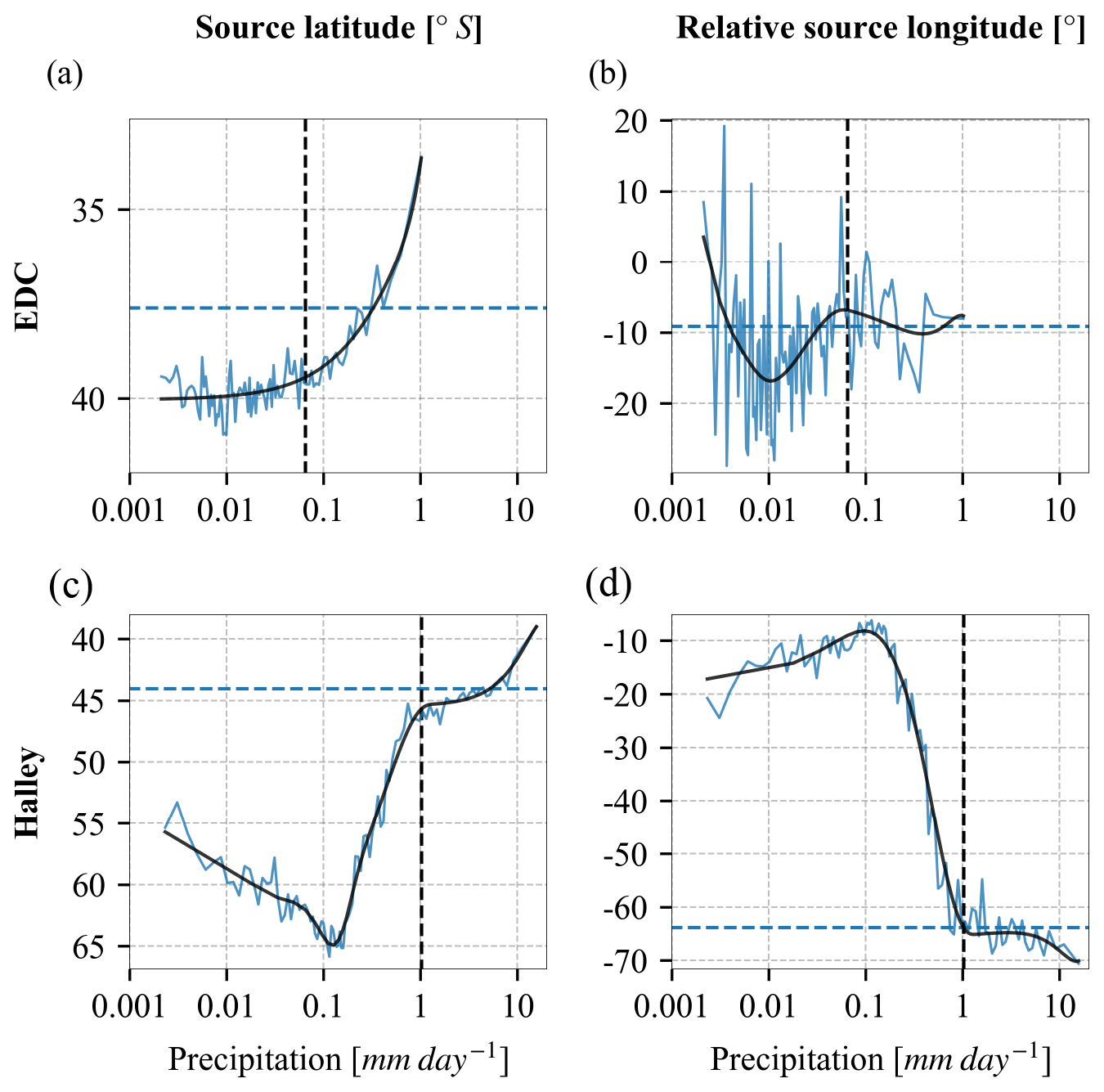
Figure 10 Variations of precipitation source properties with precipitation rates at (a–b) EDC and (c–d) Halley. Source properties include mass-weighted mean open-ocean evaporative (a, c) source latitude and (b, d) relative source longitude. Precipitation rates are calculated for each percentile of daily precipitation rates. Horizontal dashed blue lines show annual mean source properties, and vertical dashed black lines show annual mean precipitation rates. Solid black lines show spline fits to solid blue lines.

3.4 Moisture source anomalies of heavy and light precipitation

We now examine moisture source anomalies of heavy and light precipitation at two Antarctic sites and across Antarctica. We choose EDC and Halley as inland and coastal sites, respectively (Fig. B1b). After applying a precipitation threshold (see Fig. 2.3), daily precipitation rates at each site are divided into 100 percentiles. For each percentile, the precipitation rate and its contribution to the total precipitation amount can be estimated. The higher percentiles, with larger precipitation rates, contribute a larger proportion of the total site precipitation. As a result, sources of a few top percentiles exert a strong control on the mass-weighted average source properties of total precipitation.

Heavy precipitation over Antarctica depends mainly on intrusions of moist and warm maritime air masses. As underlying SST decreases during poleward moisture transport, surface evaporation might be suppressed (Thurnherr and Aemisegger, 2022). Consequently, heavy precipitation would derive its moisture from more remote regions compared to the rest of precipitation (Terpstra et al., 2021). This finding, based on a case study, is supported by our water tracing results on a climatological scale. Source–sink distance anomalies of heavy precipitation relative to the rest of precipitation are ∼ 300 km over Antarctica (Fig. 9d). By sub-regions, the source–sink distance anomalies are 290 km over EAIS, 330 km over WAIS, and 670 km over AP. Source latitude anomalies of heavy precipitation are 2.9^∘ over Antarctica, 2.9^∘ over EAIS, 3.1^∘ over WAIS, and 4.9^∘ over AP (Fig. 9a). These results quantify the degree to which heavy precipitation is related to more distant (300 km) and equatorward (2.9^∘) sources.

Similar features can be observed at the EDC and the Halley sites. At EDC, source latitude moves equatorward with increasing precipitation rates (from 40^∘ S for light precipitation to 36^∘ S for heavy precipitation), though relative source longitude indicates large fluctuations (Fig. 10). In contrast, Halley experiences two distinct precipitation regimes. For daily precipitation below ∼ 0.1 mm d⁻¹, moisture is derived from more poleward oceans (60^∘ S) and undergoes less eastward transport (by 15^∘) compared to the rest of precipitation, which indicates local sources. Above ∼ 1 mm d⁻¹, precipitation originates from more equatorward oceans (45^∘ S) and undergoes more eastward transport (by 65^∘) compared to the rest of precipitation, which represents remote sources. See also the histograms of source properties for a different type of depiction of this behaviour (Fig. B6).

Heavy precipitation also shows notable source longitude anomalies (Fig. 9b). In particular, the degree of eastward moisture advection decreases towards the Antarctic interior, reaching a ∼ 15^∘ anomaly at Dome F. This is reflective of more direct atmospheric meridional flows during heavy-precipitation events. In coastal regions, negative source longitude anomalies generally indicate more remote moisture sources and thus larger zonal moisture transport by westerlies.

Furthermore, source vel10 of heavy precipitation is typically smaller than that of the rest of precipitation (Fig. 9c; −0.32 m s⁻¹ over Antarctica, −0.36 m s⁻¹ over EAIS, −0.12 m s⁻¹ over WAIS, and −0.21 m s⁻¹ over AP). This is likely due to heavy precipitation deriving its moisture from more equatorward oceans where vel10 is generally smaller (Fig. B2) rather than less windy conditions favouring heavy precipitation.

Source property anomalies of light precipitation generally show opposite patterns to heavy precipitation: light precipitation derives moisture from more poleward regions (−2.4^∘ over Antarctica, Fig. 9e), source longitude shows diverse regional patterns (Fig. 9f), light precipitation originates from more windy oceans over large parts of Antarctica (the differences average to 0.22 m s⁻¹ over Antarctica, Fig. 9g), and light precipitation relies more on short-range moisture transport (the differences average to −290 km over Antarctica, Fig. 9h).

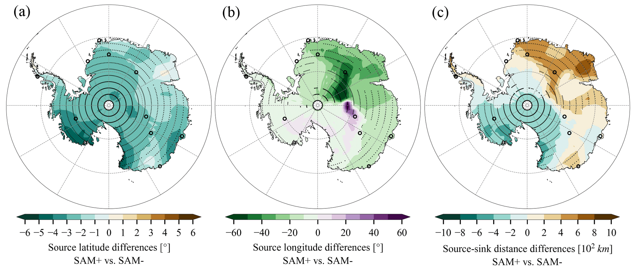
Figure 11 Differences in mass-weighted mean open-ocean evaporative (a) source latitude, (b) source longitude, and (c) source–sink distance of precipitation between SAM+ and SAM− months. Monthly mean source latitude, relative source longitude, and source–sink distance are deducted from monthly values before analysis. Stippling points represent significant differences at the 5 % significance level based on statistical tests: for source latitude and source–sink distance, Student's t test with the Benjamini–Hochberg procedure controlling false discovery rates (Benjamini and Hochberg, 1995) is adopted; for source longitude, the Watson–Williams F test for circular statistics (Watson and Williams, 1956) is employed. Positive source latitude difference means more equatorward, and positive source longitude difference means more eastward.

3.5 Impacts of SAM on moisture sources

SAM is primarily characterised by zonal winds and is thus linked to the likelihood of meridional (versus more zonal) atmospheric moisture transport (Aemisegger and Papritz, 2018). During positive SAM phases, stronger westerlies may be associated with more local storms and evaporation, whereas negative SAM favours poleward intrusions of maritime air masses from more distant sources, due to amplified Rossby waves (Stenni et al., 2010; Schlosser et al., 2016). We thus explore impacts of SAM states on Antarctic precipitation sources.

We find that negative SAM polarity is linked with more equatorward sourced moisture over most of Antarctica (Fig. 11a). The difference in source latitude between SAM+ and SAM− months is ∼ −2.4^∘ over Antarctica (−2.2^∘ over EAIS, −3.1^∘ over WAIS, and −1.2^∘ over AP). Effects of SAM polarity are also observed in source latitude of zonal mean atmospheric humidity (not shown). Above Antarctica, atmospheric humidity comes from more equatorward regions during SAM− months compared to SAM+ months, by up to 6^∘.

Impacts of SAM on source longitude vary considerably across Antarctica (−91 to 67^∘, Fig. 11b). Over large parts of Antarctica, SAM+ is linked with more eastward moisture transport by westerlies (source longitude differences: −17^∘, area-weighted over negative anomaly regions). In a few regions, e.g. near Vostok, SAM+ is connected to positive source longitude anomalies (8^∘, area-weighted over positive anomaly regions).

Correspondingly, differences in source–sink distance between SAM+ and SAM− months exhibit a dipole pattern (Fig. 11c, −600 to 800 km). Over WAIS and southern EAIS, source latitude anomalies dominate, and thus SAM+ is connected to a shorter source–sink distance (−230 km, area-weighted over negative anomalies). Over northern EAIS, source longitude anomalies dominate, and thus SAM+ is linked with a longer source–sink distance (280 km, area-weighted over positive anomalies). Whilst SAM impacts meridional moisture fluxes, the picture is not homogenous across Antarctica (Schlosser et al., 2010, 2016).

We note that SAM− months are associated with more equatorward moisture sources compared to SAM+ months, and heavy precipitation derives its moisture from more northern oceans compared to the rest of precipitation. So, we investigated whether SAM exerts control over the frequency or intensity of heavy precipitation. In the preindustrial simulation, there is no significant correlation between SAM and the intensity of heavy precipitation across Antarctica, but SAM is significantly correlated with the frequency of heavy precipitation over parts of Antarctica (not shown). Correlation patterns between SAM and heavy-precipitation frequency are similar to those between SAM and monthly precipitation, which means SAM can influence Antarctic precipitation amount through its controls on heavy-precipitation frequency.

4 Conclusions and perspectives

Antarctic precipitation plays a crucial role in determining global sea level. However, our understanding of its thermodynamic and dynamic drivers is limited. Here we tackle some of the limits of our understanding through the development and application of prescribed-region and scaled-flux water tracing diagnostics in the atmospheric GCM ECHAM6. These developments yield a powerful tool from which we can infer evaporative source regions, locations, and properties of Antarctic precipitation in a climate modelling framework.

In the preindustrial ECHAM6 simulation, the contribution to Antarctic precipitation from the open ocean is determined to be 89 %, and it is 6 % from sea ice. The open ocean south of 50^∘ S contributes 28 %, the Atlantic Ocean north of 50^∘ S contributes 10 %, the Pacific Ocean north of 50^∘ S contributes 28 %, and the Indian Ocean north of 50^∘ S contributes 23 %. Remaining contributions come from AIS (0.6 %) and other continents (4.4 %). While annual cycles of these contributions are driven by variations in meridional thermal gradients and sea ice extent, spatial patterns of the contributions are additionally influenced by the topography. Moisture from more equatorward regions is transported at higher altitudes to more central Antarctic regions, and Antarctic regions at higher elevations receive a larger proportion of precipitation from more equatorward regions compared to lower-elevation areas (Stohl and Sodemann, 2010; Bailey et al., 2019). The mass-weighted mean open-ocean evaporative source latitude of total precipitation averages to ∼ 41^∘ S over Antarctica. Precipitation at elevations above 2250 m originates from more equatorward (4^∘) oceans compared to that at elevations below 2250 m (38^∘ S vs. 42^∘ S), and EAIS precipitation is from more northern oceans by 3^∘ compared to WAIS and AP (40^∘ S vs. 43^∘ S). These results are consistent with estimates based on Lagrangian trajectories (Sodemann and Stohl, 2009), which suggest a source latitude range of 45 to 40^∘ S for precipitation over the Antarctic Plateau.

Our simulated source SST of annual mean precipitation ranges from 9.8 to 16.3 ^∘C across Antarctica, which is within the range of existing literature estimates (Petit et al., 1991; Koster et al., 1992; Delaygue et al., 2000). Source rh2m ranges from 75.6 % to 83.3 %, and source vel10 varies between 10.1 and 11.3 m s⁻¹, for precipitation across Antarctica. Source properties of Antarctic precipitation are highly related to source latitude, partly because meridional gradients of SST, rh2m, and vel10 are larger than zonal gradients at mid-latitudes. Where these properties tend to decouple from each other, this can indicate storm or seasonal controls on Antarctic precipitation sources.

Of the source properties we examine, vel10 appears to play a particularly important role in controlling Antarctic precipitation. The narrow range of annual mean source vel10 (10.1–11.3 m s⁻¹) is noteworthy, and it is consistently higher than annual mean vel10 at precipitation source locations (by an Antarctic average value of 2.1 m s⁻¹). This is likely due to higher source wind speeds driving more evaporation and thus moisture availability. Since the wind field is linked to extratropical cyclone activities, further investigation is necessary to clarify these connections.

Heavy precipitation obtains its moisture from more equatorward sources, with an Antarctic average shift in source latitude of 2.9^∘ further north and 300 km farther away compared to the rest of precipitation. This is consistent with the case-study-based finding of Terpstra et al. (2021).

As speculated by Stenni et al. (2010) and Buizert et al. (2018), negative SAM polarity is connected to more equatorward moisture provenance compared to positive SAM phases by an average of 2.4^∘ over Antarctica. These findings might explain why SAM influences heavy-precipitation frequency and thus precipitation amount.

We have identified several directions for future research. We note that the results presented here are based solely on a single model simulation. To explore the model dependence of the results, we are developing similar water tracing diagnostics in another atmospheric GCM, the UK Met Office Unified Model (Brown et al., 2012). As the coarse spatial resolution of the ECHAM6 T63 simulation might be insufficient to resolve coastal atmospheric flows and marine air intrusions, high-resolution simulations will be conducted in our future studies. While this study focuses on preindustrial conditions, moisture source changes in historical periods, palaeoclimate, and future scenarios could also be investigated. Finally, we note that the scaled-flux water tracing approach is applicable not only to Antarctic problems, but also to a range of questions associated with water cycle changes in the rapidly changing environment.

Appendix A: Implementation of scaled-flux tracers in ECHAM6 and comparison with prescribed-region tracers

Here we introduce the scaled-flux water tracing approach. The basic idea of this method follows (Fiorella et al., 2021; see their Sect. 2.1), but the implementation is designed to ensure that the tracing water budget is closed.

In the scaled-flux water tracing approach, three water tracers (wt1, wt2, wt3) are required for each evaporative source condition (e.g. source latitude). The combination of wt1 and wt2 tracks the amount of water sourced from the open ocean, while wt3 follows water evaporated from both land and sea ice. All the water in the model is therefore tracked by the sum of these three tracers.

Upward evaporative fluxes of tracer water are scaled based on evaporation conditions. For any infinitesimal evaporative flux i from the open ocean, $E_i^{\mathrm{ocn}}$, the corresponding tracer evaporative flux of wt1 is calculated as

$$\begin{array}{}\text{(A1)}& \begin{array}{rl}{E}_i^{\mathrm{wt}}(\mathrm{wt}\mathrm{1},t_i,{\mathit{\lambda }}_i,{\mathit{\varphi }}_i)& =E_i^{\mathrm{ocn}}(t_i,{\mathit{\lambda }}_i,{\mathit{\varphi }}_i)\\ & \times \mathrm{SF}(\mathrm{wt}\mathrm{1},t_i,{\mathit{\lambda }}_i,{\mathit{\varphi }}_i),\end{array}\end{array}$$

where t denotes time, λ longitude, and ϕ latitude. The scaling factor $\mathrm{SF}(\mathrm{wt},t,\mathit{\lambda },\mathit{\varphi })$ is defined for wt1 as

$$\begin{array}{}\text{(A2)}& {\displaystyle }\begin{array}{rl}& \mathrm{SF}(\mathrm{wt}\mathrm{1},t,\mathit{\lambda },\mathit{\varphi })=\\ & \left\{\begin{array}{ll}\frac{X(t,\mathit{\lambda },\mathit{\varphi })-X_{\mathrm{lower}}}{X_{\mathrm{upper}}-X_{\mathrm{lower}}}& \text{over the open ocean,}\\ \mathrm{0}& \text{over land and sea ice,}\end{array}\right.\end{array}\end{array}$$

where X is the source property of interest. X_lower and X_upper are two constants set to a lower and upper limit of X to ensure SF remains in the range of (0, 1). As arithmetic operations cannot be applied to circular data directly, tracers for source longitude are scaled based on the sine and cosine of longitude. Thereafter, source longitude is estimated according to trigonometrical functions. Values of X_lower and X_upper are defined as [−90^∘, 90^∘] for latitude, [−1, 1] for sine and cosine of longitude, [−5 ^∘C, 45 ^∘C] for SST, [0, 160 %] for rh2m, and [0, 28 m s⁻¹] for vel10.

The second water tracer (wt2) is defined such that the sum of wt1 and wt2 tracks the total open-ocean evaporation. Therefore, the evaporative flux for wt2 is given by Eq. (A1) but with the scaling factor $\mathrm{SF}(\mathrm{wt}\mathrm{2},t,\mathit{\lambda },\mathit{\varphi })$ set as

$${\displaystyle }\begin{array}{rl}& \mathrm{SF}(\mathrm{wt}\mathrm{2},t,\mathit{\lambda },\mathit{\varphi })=\\ & \left\{\begin{array}{ll}\mathrm{1}-\mathrm{SF}(\mathrm{wt}\mathrm{1},t,\mathit{\lambda },\mathit{\varphi })& \text{over the open ocean,}\\ \mathrm{0}& \text{over land and sea ice,}\end{array}\right.\end{array}$$

which gives $E_i^{\mathrm{wt}}(\mathrm{wt}\mathrm{1},t_i,{\mathit{\lambda }}_i,{\mathit{\varphi }}_i)+E_i^{\mathrm{wt}}(\mathrm{wt}\mathrm{2},t_i,{\mathit{\lambda }}_i,{\mathit{\varphi }}_i)=E_i^{\mathrm{ocn}}(t_i,{\mathit{\lambda }}_i,{\mathit{\varphi }}_i)$. Note that downward condensation fluxes of tracer water at the surface are proportional to normal water fluxes as in the prescribed-region water tracing approach.

For the atmospheric specific humidity $q_i^{\mathrm{ocn}}(t,p,\mathit{\lambda },\mathit{\varphi })$ formed from the evaporation flux $E_i^{\mathrm{ocn}}(t_i,{\mathit{\lambda }}_i,{\mathit{\varphi }}_i)$, we have the corresponding water tracer quantity,

$$\begin{array}{}\text{(A3)}& \begin{array}{rl}{q}_i^{\mathrm{wt}}(\mathrm{wt}\mathrm{1},t,p,\mathit{\lambda },\mathit{\varphi })& =q_i^{\mathrm{ocn}}(t,p,\mathit{\lambda },\mathit{\varphi })\\ & \times \mathrm{SF}(\mathrm{wt}\mathrm{1},t_i,{\mathit{\lambda }}_i,{\mathit{\varphi }}_i),\end{array}\end{array}$$

where p is the pressure level. By summing up all vapour contributions in a grid box, we obtain

$$\begin{array}{}\text{(A4)}& \begin{array}{rl}\sum _i{q}_i^{\mathrm{wt}}(\mathrm{wt}\mathrm{1},t,p,\mathit{\lambda },\mathit{\varphi })& =\sum _i\left(q_i^{\mathrm{ocn}}(t,p,\mathit{\lambda },\mathit{\varphi })\right.\\ & \left.\times \mathrm{SF}(\mathrm{wt}\mathrm{1},t_i,{\mathit{\lambda }}_i,{\mathit{\varphi }}_i)\right),\end{array}\end{array}$$

where ${\sum }_i{q}_i^{\mathrm{wt}}(\mathrm{wt}\mathrm{1},t,p,\mathit{\lambda },\mathit{\varphi })$ is the atmospheric water tracked by wt1.

By substituting $\mathrm{SF}(\mathrm{wt}\mathrm{1},t_i,{\mathit{\lambda }}_i,{\mathit{\varphi }}_i)$ from Eq. (A2) into Eq. (A4) and rearranging, we can obtain the following expression for the mass-weighted mean open-ocean evaporative source property of the atmospheric water,

$$\begin{array}{}\text{(A5)}& \begin{array}{rl}& {\displaystyle \frac{{\sum }_i\left(q_i^{\mathrm{ocn}}(t,p,\mathit{\lambda },\mathit{\varphi })\times X(t_i,{\mathit{\lambda }}_i,{\mathit{\varphi }}_i)\right)}{{\sum }_i{q}_i^{\mathrm{ocn}}(t,p,\mathit{\lambda },\mathit{\varphi })}}=\\ & {\displaystyle \frac{{\sum }_i{q}_i^{\mathrm{wt}}(wt\mathrm{1},t,p,\mathit{\lambda },\mathit{\varphi })}{{\sum }_i{q}_i^{\mathrm{ocn}}(t,p,\mathit{\lambda },\mathit{\varphi })}}\\ & \times (X_{\mathrm{upper}}-X_{\mathrm{lower}})+X_{\mathrm{lower}}.\end{array}\end{array}$$

In the above equation, ${\sum }_i{q}_i^{\mathrm{ocn}}(t,p,\mathit{\lambda },\mathit{\varphi })$ is the atmospheric water sourced from the open ocean and can be replaced with the sum of wt1 and wt2, which gives

$$\begin{array}{}\text{(A6)}& \begin{array}{rl}& {\displaystyle \frac{{\sum }_i\left(q_i^{\mathrm{ocn}}(t,p,\mathit{\lambda },\mathit{\varphi })\times X(t_i,{\mathit{\lambda }}_i,{\mathit{\varphi }}_i)\right)}{{\sum }_i{q}_i^{\mathrm{ocn}}(t,p,\mathit{\lambda },\mathit{\varphi })}}=\\ & {\displaystyle \frac{{\sum }_i{q}_i^{\mathrm{wt}}(\mathrm{wt}\mathrm{1},t,p,\mathit{\lambda },\mathit{\varphi })}{{\sum }_i{q}_i^{\mathrm{wt}}(\mathrm{wt}\mathrm{1},t,p,\mathit{\lambda },\mathit{\varphi })+{\sum }_i{q}_i^{\mathrm{wt}}(\mathrm{wt}\mathrm{2},t,p,\mathit{\lambda },\mathit{\varphi })}}\\ & \times (X_{\mathrm{upper}}-X_{\mathrm{lower}})+X_{\mathrm{lower}}.\end{array}\end{array}$$

As passive water tracers always follow normal water proportionally after evaporation, evaporative source properties of precipitation can be obtained in the same way.

The third water tracer (wt3) is used to track the water evaporated from land and sea ice; hence, $\mathrm{SF}(\mathrm{wt}\mathrm{3},t,\mathit{\lambda },\mathit{\varphi })=\mathrm{0}$ over the open ocean, and $\mathrm{SF}(\mathrm{wt}\mathrm{3},t,\mathit{\lambda },\mathit{\varphi })=\mathrm{1}$ over land and sea ice. Therefore, the combination of the three tracers tracks all the water in the model. This allows a correction to be applied at each grid point and time step to ensure that the sum of the three water tracers does not deviate from normal water in the model. Small deviations occur for numerical reasons related to partitioning normal water into multiple water tracers, and they can accumulate and propagate. We applied corrections to atmospheric tracer water to ensure their sum equals normal water. Importantly, the proportion of each water tracer does not change after corrections. These corrections are applied to both water tracing methods. The magnitude of corrections is at an acceptable level (less than 2 ‰).

The atmospheric tracer water content is initialised as a product of atmospheric normal water content and the scaling factor $\mathrm{SF}(\mathrm{wt},\mathrm{0},\mathit{\lambda },\mathit{\varphi })$.

Appendix B: Additional figures

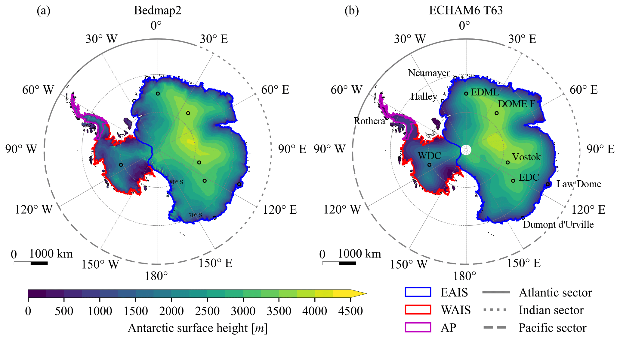
Figure B1 Antarctic surface height (a) in the observation-based Bedmap2 product (Fretwell et al., 2013) and (b) in the model simulation with T63 resolution. Definitions of EAIS, WAIS, and AP are based on the work of Eric Rignot and Jeremie Mouginot (http://imbie.org/, last access: 20 February 2023). Oceanic sectors are specified as follows: Atlantic sector (70^∘ W to 20^∘ E), Indian sector (20 to 140^∘ E), and Pacific sector (140^∘ E to 70^∘ W). Locations of five inland and five coastal sites are indicated with black empty circles. EDC stands for EPICA Dome Concordia, EDML for EPICA Dronning Maud Land, Dome F for Dome Fuji, and WDC for the WAIS Divide ice core.

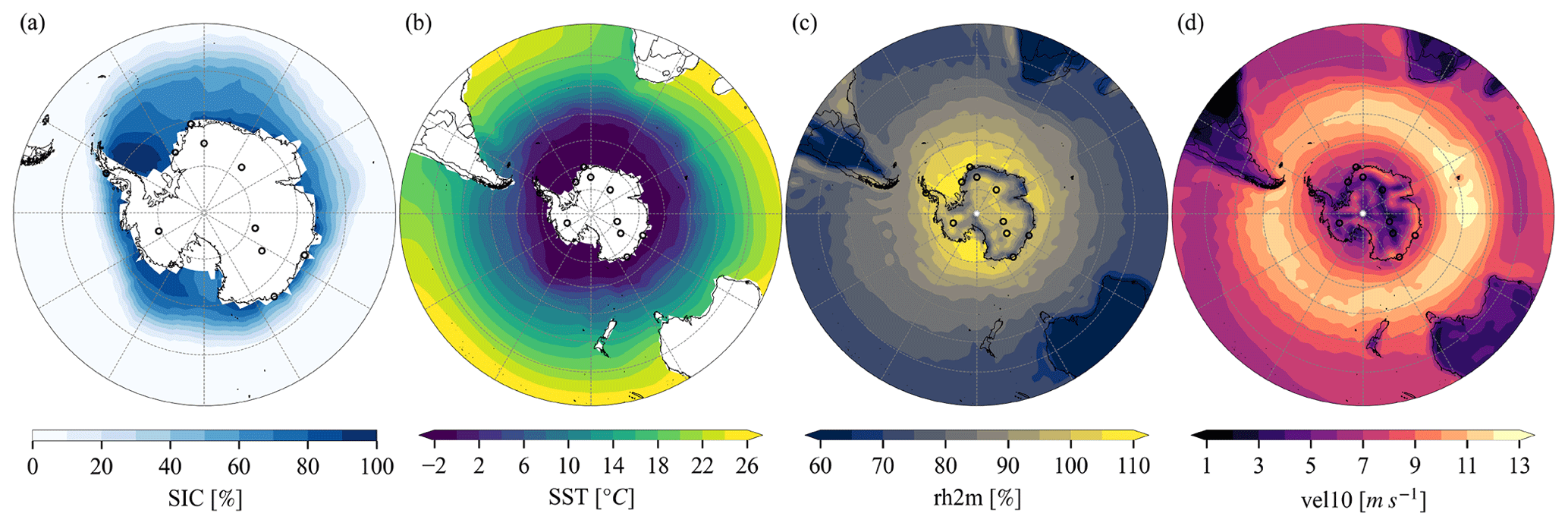
Figure B2 Annual mean (a) sea ice concentration (SIC), (b) sea surface temperature (SST), (c) 2 m relative humidity (rh2m), and (d) 10 m wind velocity (vel10) in the simulation.

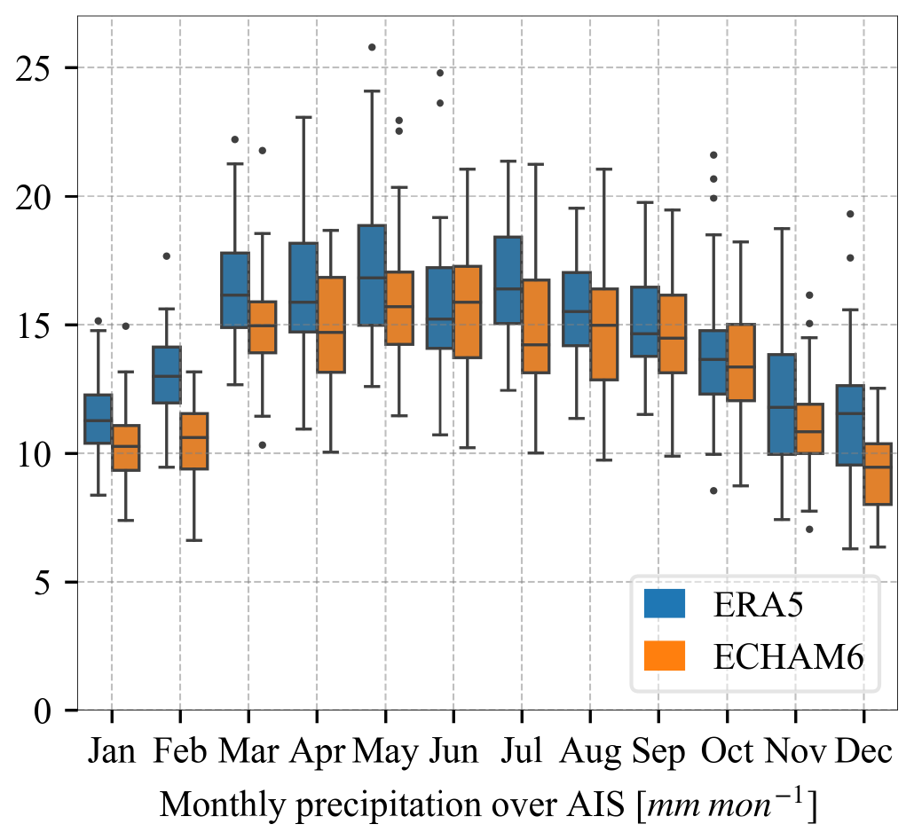
Figure B3 Monthly mean precipitation over Antarctica in ERA5 (1979–2021) and the ECHAM6 preindustrial simulation. Note that the two datasets are from slightly different climate periods.

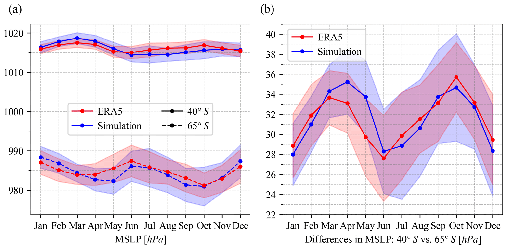
Figure B4 (a) Monthly mean zonal mean sea level pressure (MSLP) at 40 and 65^∘ S in ERA5 (1979–2021) and the simulation. (b) Differences in monthly mean zonal mean sea level pressure between 40 and 65^∘ S in two datasets. The colour shadings show 1 standard deviation.

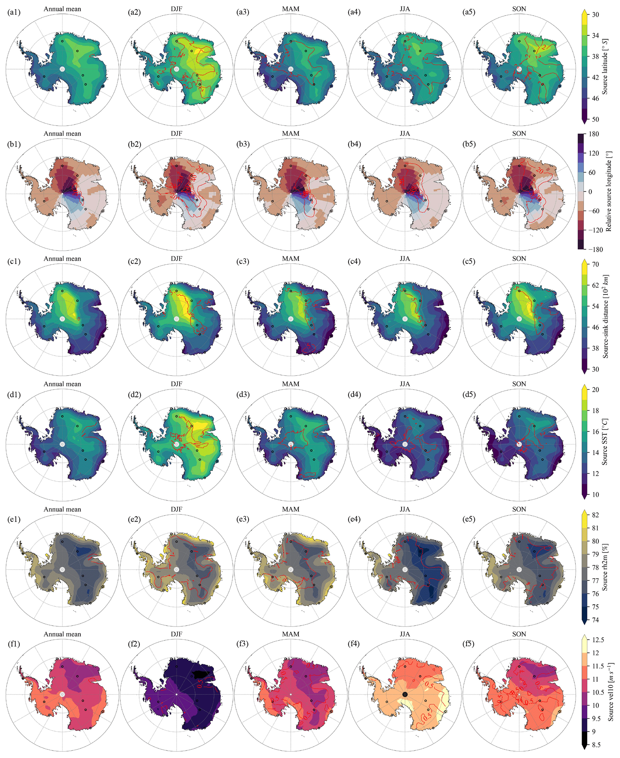
Figure B5 Mass-weighted mean open-ocean evaporative (a) source latitude, (b) relative source longitude, (c) source–sink distance, (d) source SST, (e) source rh2m, and (f) source vel10 of the annual mean (the first column) and seasonal mean (the second to fifth columns) precipitation. Red lines show contours of 1 standard deviation. DJF refers to December–January–February, MAM to March–April–May, JJA to June–July–August, and SON to September–October–November.

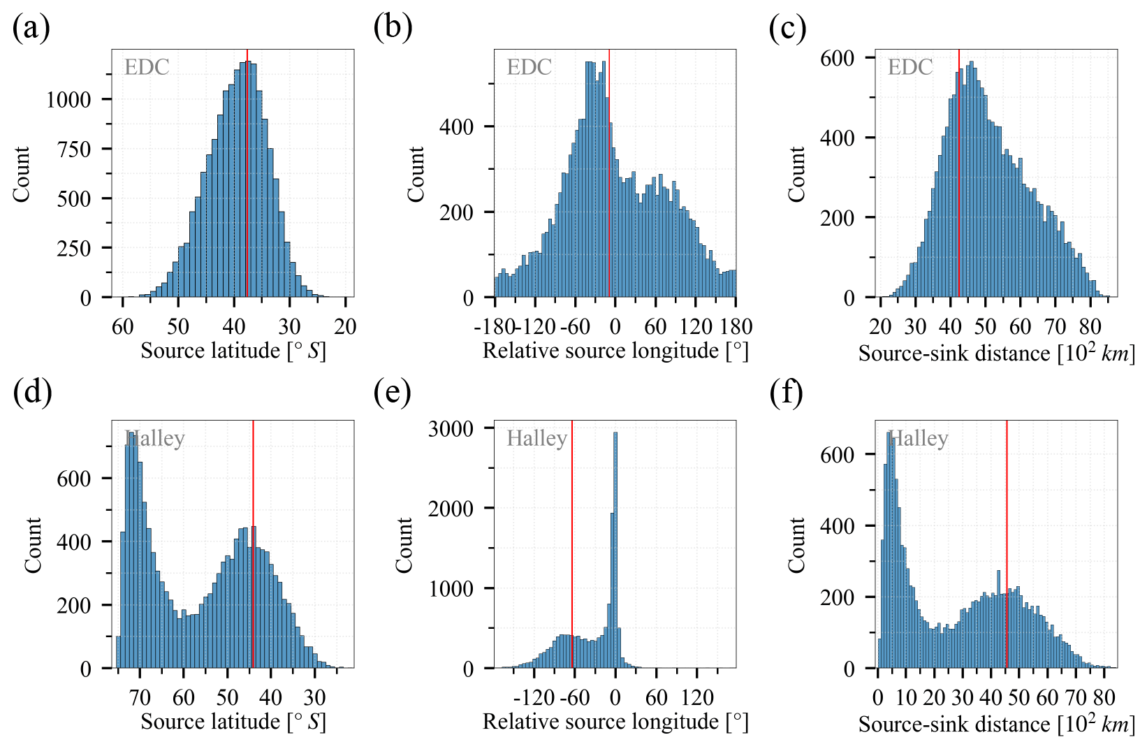
Figure B6 Histograms of source properties of daily precipitation at (a–c) EDC and (d–f) Halley. Source properties include mass-weighted mean open-ocean evaporative (a, d) source latitude, (b, e) relative source longitude, and (c, f) source–sink distance. Vertical red lines represent source properties of annual mean precipitation.