the Creative Commons Attribution 4.0 License.
the Creative Commons Attribution 4.0 License.
Land surface temperature trends derived from Landsat imagery in the Swiss Alps
Deniz Tobias Gök
Dirk Scherler
Hendrik Wulf
The warming of high mountain regions caused by climate change is leading to glacier retreat, decreasing snow cover, and thawing permafrost, all of which have far-reaching effects on ecosystems and societies. Landsat Collection 2 provides multi-decadal land surface temperature (LST) data, principally suited for large-scale monitoring at high spatial resolution. In this study, we assess the potential to extract LST trends using Landsat 5, 7, and 8 time series. We conduct a comprehensive comparison of both LST and LST trends with data from 119 ground stations of the Intercantonal Measurement and Information System (IMIS) network, located at high elevations in the Swiss Alps. The direct comparison of Landsat and IMIS LST yields robust satellite data with a mean accuracy and precision of 0.26 and 4.68 K, respectively. For LST trends derived from a 22.6-year record length, as imposed by the IMIS data, we obtain a mean accuracy and precision of −0.02 and 0.13 K yr−1, respectively. However, we find that Landsat LST trends are biased due to unstable diurnal acquisition times, especially for Landsat 5 and 7. Consequently, LST trend maps derived from 38.5-year Landsat data exhibit systematic variations with topographic slope and aspect that we attribute to changes in direct shortwave radiation between different acquisition times. We discuss the origin of the magnitude and spatial variation of the LST trend bias in comparison with modeled changes in direct shortwave radiation and propose a simple approach to estimate the LST trend bias. After correcting for the LST trend bias, the remaining LST trend values average between 0.07 and 0.10 K yr−1. Furthermore, the comparison of Landsat- and IMIS-derived LST trends suggests the existence of a clear-sky bias, with an average value of 0.027 K yr−1. Despite these challenges, we conclude that Landsat LST data offer valuable high-resolution records of spatial and temporal LST variations in mountainous terrain. In particular, changes in the mountain cryosphere, such as glacier retreat, glacier debris cover evolution, and changes in snow cover, are preserved in the LST trends and potentially contribute to improved prediction of permafrost temperatures with large spatial coverage. Our study highlights the significance of understanding and addressing biases in LST trends for reliable monitoring in such challenging terrains.
- Article
(7933 KB) - Full-text XML
-
Supplement
(24289 KB) - BibTeX
- EndNote
The Earth's surface temperature at the land–atmosphere interface is a key parameter of the surface energy budget and influences a range of biological, chemical, and physical processes within the critical zone (e.g., Brantley et al., 2007). It reflects both climate change and land surface processes and is defined as an essential climate variable by the World Meteorological Organization (Bojinski et al., 2014). Increasing surface temperature is expected to have a severe adverse impact on ecosystems, human health, and infrastructure (IPCC, 2023). With time, surface warming propagates to greater depths, resulting in additional changes. High mountain regions that host glaciers, snow cover, and permafrost are particularly sensitive to increasing temperatures. Where mean annual ground temperatures rise to above 0 °C, permafrost thaws, thereby destabilizing steep hillslopes (Gruber and Haeberli, 2007; Huggel, 2009; Allen et al., 2009). Indeed, increased rockfall activity and several recent significant slope failures in the European Alps (Gruber et al., 2004; Harris et al., 2009; Walter et al., 2020) have been linked to permafrost thaw. Such catastrophic events pose serious hazards to both people and infrastructure in numerous mountain ranges on Earth. Monitoring Earth's surface temperature and its spatiotemporal variation therefore significantly contributes to the improved prediction of the impacts of global warming. However, ground-based instrumental monitoring of surface temperature is laborious and difficult to implement over large regions and in remote mountainous areas with steep hillslopes. Therefore, the spatial coverage of station-based surface temperature data is limited, especially when it comes to long-term records.
Satellite platforms equipped with thermal infrared sensors allow the land surface temperature (LST) to be measured at a range of spatial and temporal resolutions and have long been used in a variety of research fields (Li et al., 2013; Hulley et al., 2019; Reiners et al., 2023; Li et al., 2023). Temporal LST analysis for climate change studies or environmental monitoring requires multi-decadal time series data, which often involves the challenge of maintaining the temporal coherence of thermal data (Kuenzer and Dech, 2013). Many LST studies rely on data from the Moderate Resolution Imaging Spectroradiometer (MODIS) sensor on board the Terra and Aqua satellites (Reiners et al., 2023). MODIS LST records are temporally consistent (Hulley and Hook, 2011), and LST trends have recently been derived globally (Sobrino et al., 2020). However, the relatively coarse spatial resolution of the thermal bands (1000 m) restricts the applicability of MODIS LST in high mountainous regions, where the steep terrain results in large spatial gradients in surface temperatures. In addition to altitudinal gradients in temperature, due to the decreasing air temperature, temperature variations also exist in response to variable exposure to the sun.
As the robustness of trends increases with longer time series, LST records from the Advanced Very High Resolution Radiometer (AVHRR) with 1000 m spatial resolution and the Landsat program (60–120 m spatial resolution) are particularly useful for this purpose (Prata, 1994; Gutman and Masek, 2012). Both suffer, although in a different manner, from orbital drift effects, causing the acquisition time to vary over time (Julien and Sobrino, 2022; Zhang and Roy, 2016). Orbital drift corrections for AVHRR LST time series are continuously being developed (e.g., Gutman et al., 1999; Jin and Treadon, 2003; Dech et al., 2021; Julien and Sobrino, 2022), as the daily temporal resolution allows for unique insights into the long-term dynamics of LST. Landsat, with its lower temporal but higher spatial resolution, has so far been underutilized in time series analysis (Fu and Weng, 2015). The recently released Landsat Collection 2, with improved radiometric calibration and geolocation information (Crawford et al., 2023), provides consistently generated LST data (Malakar, 2018). Landsat-derived LST time series therefore present a unique opportunity to explore the dynamics of high mountain landscapes in response to climate change and human land cover modifications.
For instance, recently published LST trends of glacier surfaces in High Mountain Asia show enhanced surface warming trends due to supraglacial debris cover and its expansion (Ren et al., 2024). Spatial patterns in LST trends are also expected in areas of seasonal snow cover. At altitudes near the 0 °C isotherm in particular, small changes in air temperature can have a significant impact on snow cover (Pepin and Lundquist, 2008). Observations show that in the European Alps snow cover declines in extent, duration, and depth (Matiu et al., 2021) with vegetation, expanding into higher elevations and thus changing the surface albedo (Rumpf et al., 2022). Furthermore, because mountain permafrost temperatures vary in response to changes in air temperature and snow cover (Smith et al., 2022), spatial patterns in LST and LST trends have the potential to inform expected spatial variations in permafrost temperature, depth, and extent. Despite sufficiently long records and the high spatial resolution of Landsat observations, deriving LST trends is complicated as acquisition times have changed by up to 1 h (Roy et al., 2020) due to orbit changes over the last few decades (Zhang and Roy, 2016).
Here, we explore the opportunities of monitoring LST trends in steep mountainous regions using Landsat Collection 2. We first assess the reliability of Landsat-derived LST and LST trends by comparison with ground observations from the Intercantonal Measurement and Information System (IMIS) network, which provides comparable radiometric surface temperatures at high-elevation sites across the Swiss Alps (Fig. 1). We then calculate spatially distributed LST trends and identify a spatially variable bias that we associate with orbital drift of the satellites. We analyze the magnitude of and spatial variation in this bias and present a simple approach to correct for it. Additionally, we address issues related to the clear-sky bias and explore opportunities and limitations of studying cryosphere changes using the corrected Landsat LST trends.
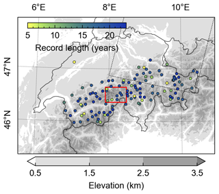
Figure 1Intercantonal Measurement and Information System (IMIS) network of automated weather stations distributed across the Swiss Alps. The presented 115 stations provide radiometric surface temperatures at 30 min intervals with time spans greater than 5 years, indicated by the inset color. The red rectangle identifies the upper Rhône Valley shown in Fig. 7. The dashed black rectangle indicates the Landsat footprint at path 194 and row 27, referred to in Fig. 2.
2.1 Landsat-derived LST
Landsat Collection 2 (C2) Level-2 science products provide multi-decadal observational remote sensing data that are geometrically and radiometrically consistent and have harmonized quality assessment bands (Dwyer et al., 2018). We used Google Earth Engine (GEE) to analyze LST data (Malakar et al., 2018) from the Landsat 5 Thematic Mapper (TM), Landsat 7 Enhanced Thematic Mapper Plus (ETM+), and Landsat 8 Thermal Infrared Sensor (TIRS) (hereafter LT05, LE07, and LC08) covering a time span from 1984 to 2022. The native spatial resolutions of LT05 (120 m), LE07 (60 m), and LC08 (100 m) were resampled in Collection 2 to 30 m, which is the spatial resolution that we used. Throughout the study, we use degrees Celsius (°C) for absolute temperatures and kelvin (K) for temperature differences and rates.
The Landsat C2 LST calculation is based on a single-channel algorithm (Malakar et al., 2018) that relies on only one thermal infrared band and that has been widely used to retrieve LST from Landsat data (Jiménez-Muñoz and Sobrino, 2003; Cook et al., 2014). The conversion of at-sensor radiometric temperature to LST requires an atmospheric correction and knowledge of the surface emissivity. The atmospheric correction in the Landsat C2 LST calculation is based on the total column water vapor derived from National Centers for Environmental Prediction (NCEP) atmospheric reanalysis data (Kalnay et al., 1996). Mean emissivity estimates over the time period 2000–2008 are based on the Advanced Spaceborne Thermal Emission and Reflection Radiometer Global Emissivity Dataset (ASTER GED) (Hulley et al., 2015) and temporally adjusted using Landsat-derived normalized difference vegetation index (NDVI) and normalized difference snow index (NDSI). Inspection of the ASTER GED reveals several artifacts, which appear to align with artifacts in the Landsat LST data. To avoid erroneous LST data and mask out clouds in the Landsat images, we applied several filters and masks that we describe in more detail in Sect. 2.3.
The scene acquisition time of Landsat for the Swiss Alps lies mostly between 09:30 and 10:30 UTC. Figure 2 shows the acquisition times from the different Landsat sensors during the study period. While LC08 has a relatively stable acquisition time, LE07 shows slightly continuous drift before 2018 and strong drift after 2018 due to depleted onboard fuel resources (Qiu et al., 2021). LT05 on the other hand shows both sporadic and continuous orbit changes that lead to significant variations in acquisition time (Zhang and Roy, 2016). Although orbit variations are often due to sporadic orbit keeping maneuvers, a gradual increase in overpass times is evident too (Roy et al., 2020). When fitting a linear model to all satellites together (but excluding LE07 data after 2018 due to strong orbital decay), the acquisition time increased from approximately 09:29 UTC in 1984 to 10:16 UTC in 2022 (Fig. 2, dotted line). We expect that LST trends derived from the 38.5-year time series are likely biased by the progressively delayed acquisition times, probably towards more positive values, due to gradual warming of the land surface in the morning. Because different acquisition times also lead to geometric changes in the sun–target–sensor configuration, this bias may additionally vary with the slope and aspect of the topography. We describe our approach to analyzing this issue in Sect. 2.4.
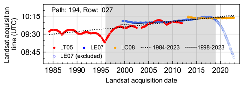
Figure 2Acquisition times (UTC) of Landsat LT05 (red), LE07 (blue), and LC08 (orange) at path 194 and row 027. LE07's noticeable orbital drift after 2018 (empty blue circles) causes a significant shift in revisit timing and has been excluded from the analysis. Linear regression lines (dotted and dashed) depict acquisition time trends, with and without abrupt LT05 orbit changes prior to 2000. The gray-shaded area indicates the time period for which IMIS station data exist, although with variable record lengths.
2.2 IMIS-derived LST
We evaluated the Landsat-derived LST data by comparing them with in situ surface temperature measurements from automated weather stations of the IMIS network. The IMIS network was set up by the Swiss Federal Institute for Snow and Avalanche Research (SLF) and consists of 186 stations distributed across the Swiss Alps. We used a subset of 119 stations (Table S1) that provide radiometric surface temperature records in 30 min intervals. The IMIS stations measure radiometric surface temperature with an infrared sensor measuring in a wavelength range of 7 to 20 µm (David Liechti, personal communication, 2023). The record length per station varies, with the longest record covering a period from 1996 to 2019 (Fig. 1). The IMIS stations are located between 1258 and 2953 m elevation above sea level and are usually installed on flat to gently sloping ground. As the stations are primarily used for snow monitoring, the reported surface temperature is calibrated using an emissivity of 0.98 (for snow), which may thus introduce a bias towards colder temperatures during snow-free conditions. Because the transition between snow-covered and snow-free conditions cannot be unambiguously determined based on the IMIS data alone and because of unknown actual emissivity values of the ground surface, we refrained from efforts to correct this bias. For a surface temperature of 15 °C, a change in emissivity of 0.01 would result in a temperature change of 0.73 K (Kuenzer and Dech, 2013). This bias decreases for lower LST values. Despite potential measurement deviations under snow-free conditions, the IMIS stations measure radiometric surface temperatures and are thus well suited for comparison with Landsat-derived LST. Additionally, the high temporal resolution of the IMIS data allows us to compare LST clear-sky and cloudy-sky conditions using the Landsat overpass times. We expect the large difference in spatial resolution to introduce additional uncertainty as Landsat most likely provides a mixed-pixel signal of potentially spatially varying LSTs compared to the IMIS data.
2.3 LST processing and trend estimation
For the studied period and the chosen Landsat sensors, we obtained for each 30 m pixel in the co-registered image collection several hundred LST observations scattered across different times of a year. We used a harmonic model including a linear trend (Eq. 1) to perform an ordinary least squares regression (Shumway and Stoffer, 2013; Fu and Weng, 2015) on the LST time series data in order to estimate (1) the mean annual LST (MALST), (2) the annual LST amplitude, (3) the long-term LST trend, and (4) the phase shift:
where β0 is the mean annual LST (K), β1 is the slope (K yr−1) of the linear trend, t is the time in years, A is the amplitude (K), ω is the frequency (equal to one for one cycle per year), and φ is the phase. The harmonic term can be decomposed into a sine and cosine term, and Eq. (1) is thus linearized to
where β2 and β3 are the newly introduced coefficients that are equal to Acos(φ) and Asin(φ), respectively. GEE allows for ordinary least squares regression of Eq. (2) and thus the determination of the four coefficients β0 to β3. We acknowledge that LST time series may contain abrupt changes due to land cover change, for example, which may not be well captured by a linear model (Zhu and Woodcock, 2012). Different approaches have been proposed to detect such changes and simultaneously obtain trend values (see the recent review by Li et al., 2022). However, the change detection approaches currently available in GEE are more limited (Kennedy et al., 2010; Zhu and Woodcock, 2012), and, as shown later, the segmentation of the time series affects our ability to account for LST trend bias due to orbital drift.
Prior to fitting Eq. (2) to the Landsat LST data, we implemented filters to mask (1) duplicate LST observations with the same date that result from along-track overlapping Landsat scenes and (2) cloud-contaminated pixels. The along-track duplicates were removed by creating image pairs of each Landsat scene and its temporal neighbor in the same path and masking the overlapping region of the adjacent scene. The pairs of subsequent Landsat scenes were identified by a difference in acquisition time of less than 100 s, which is small enough to select only the scene following directly after. Cloud masking was done using the Landsat C2 pixel quality assessment (QA) band cloud flag with at least medium confidence (Dwyer et al., 2018; Zhu and Woodcock, 2012). Although the cloud flag of the QA band provides good accuracy (Foga et al., 2017), bright surfaces, such as snow and ice in high mountain settings, can still be challenging. Predominantly in LT05 data, we find extremely low LST values, which are likely clouds that were not captured by the cloud detection algorithm. To overcome this issue, we applied an additional filter that masks outliers by applying a threshold to the residuals between the modeled and observed LST. We first calculated the β coefficients on the cloud-filtered data, including potential outliers missed by the QA cloud flag, and then uploaded them to GEE. In a second step, we predicted for each Landsat acquisition time the corresponding LST using the uploaded β coefficients (Eq. 2) and applied a threshold of ±30 K to the residuals to mask extreme LST values (due to undetected clouds or wildfires, for example) that might otherwise bias the LST trend (cf. Weng and Fu, 2014). The procedure was applied to the complete Landsat time series data. Figure 3 shows an exemplary LST time series from each sensor, the harmonic model with a linear trend, the residuals, and the filtered outliers at the location of IMIS station AMD2. Identical figures from all IMIS locations can be found in the Supplement File S2.
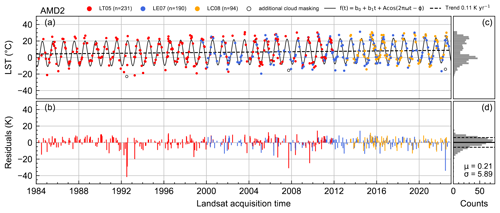
Figure 3Time series of Landsat LT05- (red), LE07- (blue), and LC08-derived (orange) land surface temperature (LST) (a) at location 47.17° N, 9.15° E (IMIS station AMD2). The harmonic model (solid sinusoidal line) was derived by least squared regression including a linear trend component (dashed line). Outliers (empty circles) were detected by applying a threshold of ±30 K to the (b) residuals and were removed from further analysis. Panels (c) and (d) show the distribution of the LST and residuals, respectively.
To assess the reliability of the Landsat-derived LSTs and LST trends, we compared them with LST data derived from the IMIS network. We first extracted the Landsat LST time series at the locations of the IMIS stations. As IMIS records are only available in 30 min intervals, we linearly interpolated LSTs at the Landsat acquisition times to obtain comparable LST time series of equal length. Based on Eq. (2), we derived the mean annual LST, the LST amplitude, the phase of the harmonic oscillation, and LST trends for both datasets. We further assessed the sensitivity of LST trends to the LT05, LE07, and LC08 sensors by comparing data from each sensor with the corresponding IMIS LST data, where the observation periods overlap. Because the temporal overlap of the individual Landsat sensors and the IMIS data varies, this comparison also results in different record lengths.
We used Student's t test to draw a statistical inference for the regression slope and evaluate the significance of LST trends (Muro et al., 2018). Pixels with non-significant trends (p values < 0.05) were flagged. Note that the comparison of LST trends between Landsat and IMIS data, as well as the spatial analysis of LST trends in relation to the LST trend bias, is based on all trend data and does not require statistical significance of trend values.
2.4 LST trend bias analysis
We expect the LST trend to be biased due to the variations in acquisition time caused by orbital change of the satellites (Fig. 2). Within the 47 min time difference in image acquisition between the beginning and the end of the 38.5-year Landsat observation period, the sun's position, and thus also the solar zenith angle, changes notably, modifying the amount of incoming shortwave radiation received by the surface. In mountainous terrain with variably steep and exposed topography, we expect this effect to be spatially non-uniform. Based on the fitted linear model of the acquisition time, we analyzed changes in the incoming direct solar radiation (ΔSin) for the Swiss Alps using the “insol” functional library (Corripio, 2003). We studied the relationship of LST trends and ΔSin with topography by aggregating mean values for 2° slope and 10° aspect sections derived from the 10 m resolution Copernicus digital elevation model (Copernicus DEM, 2022). Prior to averaging LST trends, we excluded glaciers and recently deglaciated areas using a mask based on glacier outlines from the Randolph Glacier Inventory v6 (RGI Consortium, 2017), which we expanded by 10 pixels in the 30 m resolution LST trend images. Additionally, we excluded all regions below 1700 m elevation, which are likely influenced by anthropogenic land cover changes (Rumpf et al., 2022).
2.5 Validation metrics
The LST data used in this study, obtained from the Landsat C2 archive, are based on three different sensors (LT05, LE07, and LC08) and auxiliary datasets such as the ASTER GED and NCEP reanalysis data. Since both of these datasets have their limitations, it is important to validate LST data to ensure their accuracy and reliability. We compared the Landsat-derived LST measurements with in situ LST measurements from the IMIS stations at the Landsat acquisition time. We followed the Land Surface Temperature Product Validation Best Practice Protocol (Guillevic et al., 2017) by using metrics of accuracy, precision, and uncertainty to report LST validation results. The accuracy (μ), as a measure of the systematic error, is given by the arithmetic mean of the difference between the satellite-derived LST and the in-situ-measured reference LST (ΔLSTref). The precision (σ) describes the spread of the LST around the expected value (ΔLSTref) and can be approximated by the standard deviation. The uncertainty is given by the root mean square error (RMSE) and describes the dispersion of the LST values. Because the accuracy and precision of LST data can be strongly affected by outliers, we also report the median of the ΔLSTref for the accuracy and the median absolute deviation of the residuals for the precision as additional validation metrics (Guillevic et al., 2017). We apply these validation metrics to both the LST data and the LST trends. We emphasize that in our study the term validation may be slightly misleading as it suggests that the ground-based IMIS measurements provide the correct LST values. However, we note that even the IMIS data are most likely biased during snow-free conditions (see Sect. 2.2) and subject to measurement uncertainties. In addition, the different footprints of the ground-based (∼ 10 cm) and spaceborne (∼ 10–100 m) measurements allow for deviations due to spatial heterogeneity in LST. We come back to this issue in the Discussion section. Nevertheless, we argue that the comparison of these datasets is a valuable effort and that consistency between both temperature measurements provides confidence.
3.1 LST comparison
For the comparison of Landsat-derived LST with ground-based LST from the IMIS network, we interpolated IMIS LSTs at the Landsat acquisition time. In total 44 981 Landsat observations are available for comparison with IMIS observations. The LST data from all three Landsat sensors are scattered around the 1:1 line in comparison with the IMIS data (Fig. 4a–d). At around 0 °C IMIS LST, the spread in Landsat-derived LST is considerably larger than that of the observations at the IMIS stations. It furthermore appears that LSTs derived from each Landsat sensor tend to be slightly warmer for LSTs above 0 °C compared to those below 0 °C. Mean- and median-based metrics of accuracy (μ), precision (σ), and uncertainty (RMSE) between Landsat and IMIS LST for each sensor and the entire time series are shown in Fig. 4 and Table 1. The accuracy (μ) ranges from +0.05 K (LC08) to +0.36 K (LE07) and indicates a slight positive bias. The precision (σ) ranges from 4.04 (LE07) to 6.06 K (LT05). Considering data from all three sensors together (Fig. 4d), the accuracy is +0.26 K, the precision is 4.69 K, and the uncertainty is 4.7 K (Table 1). Considering median values, the precision improves but the accuracy deteriorates.
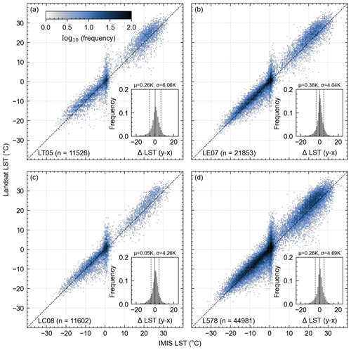
Figure 4Comparison of Landsat-derived land surface temperature (LST) with IMIS LST for (a) the Thematic Mapper (LT05); (b) the Enhanced Thematic Mapper Plus (LE07); (c) the Thermal Infrared Sensor (LC08); and (d) LT05, LE07, and LC08 together (L578). The colors denote the number of data points by decadal logarithm. The inset figures show histograms of LST residuals, with ΔLST being Landsat LST–IMIS LST.
3.2 LST trend comparison
We also compared Landsat-derived LST trends with trends derived from IMIS LST data interpolated at Landsat observation times for each sensor and the complete time series (Fig. 5, Table 2). We excluded stations with record lengths of less than 5 years. Short time series result from different temporal overlaps between the IMIS records and Landsat sensors, in particular LT05 and LC08 (Fig. 5a, c). These show large scatter around the 1:1 line compared to trends derived from longer time series, resulting in relatively large uncertainties (Table 2). Therefore, amongst the different sensors, LE07 provides the most reliable results (Fig. 5b), with better accuracy and precision (Table 2), due to the large temporal overlap with the IMIS data. Consequently, our comparison of trends derived from all sensors with IMIS-derived LST trends (Fig. 5d) is primarily dominated by LE07. Considering data from all three sensors together, the accuracy is −0.02 K yr−1, and the precision is 0.13 K yr−1, improving considerably when referring to median values.
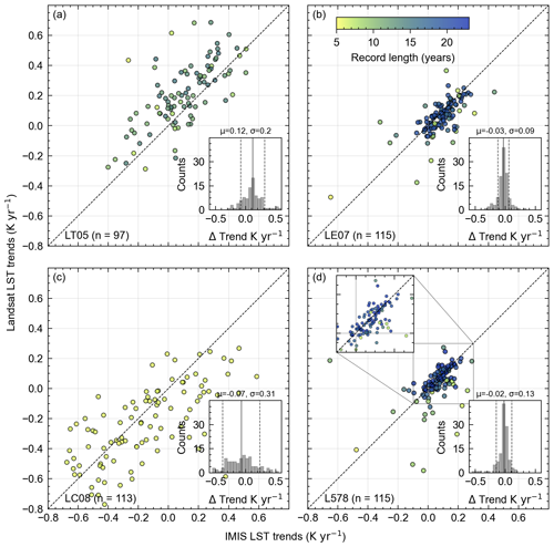
Figure 5Comparison of Landsat-derived land surface temperature (LST) trends with IMIS LST trends for the (a) Thematic Mapper (LT05); (b) Enhanced Thematic Mapper Plus (LE07); (c) Thermal Infrared Sensor (LC08); and (d) LT05, LE07, and LC08 together (L578). Stations with a record length (marker color) of less than 5 years have been omitted. Trend residuals (Landsat LST trends and IMIS LST trends) together with the accuracy (μ) and precision (σ) values are shown in the inset histograms. Note the strong impact of record length on the comparison of LST trends.
3.3 Spatiotemporal variations in LST
We applied Eq. (2) to the Landsat LST time series (LT05, LE07, and LC08) across Switzerland using GEE. The model results are presented as maps of the mean annual land surface temperature (MALST), the LST amplitude, the phase of the harmonic oscillation, and the LST trend in Fig. 6, with a focus on the upper Rhône Valley shown in Fig. 7. The presented MALST values are for the year 2000 and range from −25 to +25 °C. We consistently observe the highest MALST values at low elevations and the lowest at high elevations, where snow- and ice-covered areas range from 0 to −20 °C. As seen in the detailed map in Fig. 7a, MALST values show reasonable spatial variations with terrain aspect, and no significant processing artifacts are present. East-facing slopes consistently display higher MALST compared to west-facing ones, which aligns with expectations due to the late morning overpass of the Landsat satellites (Fig. 7a). Data gaps, which are most evident in southern Germany in Fig. 6, are due to data gaps in the ASTER GED data and are consistent across all variables. LST amplitude values range between 3 and 25 K (Fig. 6b), with the lowest values where snow or ice cover is present year-round. High-amplitude values are found in regions with seasonal snow cover that also heat up during the summer (Fig. 7b). The phase of the harmonic oscillation (Fig. 7c) shows spatial variations in seasonal shifts, which we report as the day of the year with the highest (peak) temperature in the annual LST cycle. The phase values display an altitudinal gradient (Fig. 6c) with a slight aspect dependence (Fig. 7c).
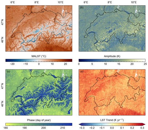
Figure 6Landsat land surface temperature (LST) time-series-derived (a) mean annual LST (MALST), (b) LST amplitude, (c) phase of the harmonic oscillation, and (d) LST trend across Switzerland and adjacent areas.
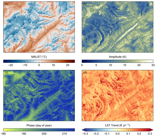
Figure 7Landsat land surface temperature (LST) time-series-derived (a) mean annual LST (MALST), (b) LST amplitude, (c) phase of the harmonic oscillation, and (d) LST trend across the upper Rhône Valley.
Averaged across the entire study area, the mean LST trend is 0.14 K yr−1 with a 5th and 95th percentile of 0.08 and 0.21 K yr−1, respectively (Fig. 6d). Areas with a high population density often appear to exhibit trend values exceeding 0.2 K yr−1. Notably, the highest trend values are observed in areas where retreating glaciers expose sediment or bedrock (Fig. 7d). Compared to the MALST, the LST amplitude, and the phase of the harmonic oscillation, the LST trend values display more artifacts. Subtle but systematic across-track jumps in LST trends are visible in the northeast of the map in Fig. 6d. These artifacts align with the Landsat orbit and variations in the number of observations due to overlapping scenes from adjacent orbital tracks (Fig. S3.1; see Supplement). Similarly, the post-2003 Landsat LE07 scan line corrector failure induces across-track stripes in the number of LST observations that also appear in some parts of the LST trend maps (only faintly visible on some glacier surfaces in Fig. 7d). These patterns in LST trend values are consistent with the sensitivity to record length we observed in our comparison of Landsat- and IMIS-derived LST trends (Sect. 3.2). We further discuss this point in Sect. 4.1. Finally, LST trends in the detailed map display an aspect dependency, with generally lower values on east-facing slopes and higher values on west-facing slopes (Fig. 7d). Regions with flat topography (as in the foreland), wide valleys, or lakes show more continuous trend values. We suspect that this effect is related to the shift towards later acquisition times and thus to variations in the solar zenith angle over the 38.5-year Landsat record. In the following section we examine this trend bias in more detail using IMIS station data.
3.4 LST trend bias
We point out in Sect. 2.1 that Landsat acquisition times have changed between 1984 and 2022. Approximating this change by a linear model for the acquisition time yields a time difference of 47 min over a period of 38.5 years (from 09:29 UTC in 1984 to 10:16 UTC in 2022; Fig. 2). To estimate how much of an LST difference we can expect to result purely from this 47 min delay in image acquisition, we exploit the high-temporal-resolution IMIS data by calculating for every day and every IMIS station the LST difference between 10:16 and 09:29 UTC. The daily LST differences (ΔLST) show a bimodal distribution (Fig. 8), which we separated using bimodal Gaussian regression. During melting periods, snow surfaces remain locked at the melting point, and ΔLST values are essentially zero (blue curve). The remaining ΔLST values are normally distributed (red curve) with a mean ΔLST of 1.72 K and a standard deviation of 0.93 K. The mean ΔLST of the full distribution is 1.55 K, which, over a 38.5-year period, suggests an average LST trend bias of 0.04 K yr−1. However, the IMIS stations are located on flat to gently sloping terrain, and the LST trend bias varies with topography.
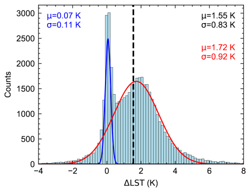
Figure 8Bimodal distribution of IMIS-derived land surface temperature differences (ΔLST) in daily LST interpolated at 09:29 and 10:16 UTC. The mean (μ) ΔLST of the full distribution is 1.55 K, and the standard deviation (σ) is 0.83 K, which, over a 38.5-year period, suggests an average LST trend bias of 0.04 K yr−1 over flat and gently sloping terrain where IMIS stations are typically located.
The influence of topographic slope and aspect on the LST trends is shown by aggregated mean values for 2° slope and 10° aspect bins in Fig. 9c. For slope angles above ∼ 10°, LST trends are generally lower on east-facing slopes, whereas they are higher on west-facing slopes. Mean LST trend values for slope angles above 75° are noisy due to very few samples (pixels) and were excluded from analysis. We compared this pattern with modeled differences in incoming solar radiation between 09:29 and 10:16 UTC (ΔSin) for the first of all months of the year using terrain parameters from the DEM of our study area. In Fig. 9d we show the pattern for July, which turned out to resemble the LST trend pattern the most, although differences in ΔSin patterns between May and September are generally small.
Overall, we find large similarities in the general pattern of how mean LST trends and ΔSin vary with slope and aspect (Fig. 9c, d; note that the color bar in d diverges, while the other one is continuous). Specifically, the cross sections shown for slope angles of 30 and 50° (Fig. 9e, f) highlight the similar sinusoidal variation in LST trend and ΔSin with aspect. As expected, LST trend and ΔSin variations with aspect are low for slope angles < 10°. However, while the average ΔSin value for any given slope and across all aspects is relatively similar, this is not the case for LST trends. Here, we observe higher trend values for small slope angles when averaged across all aspects compared to higher slope angles.
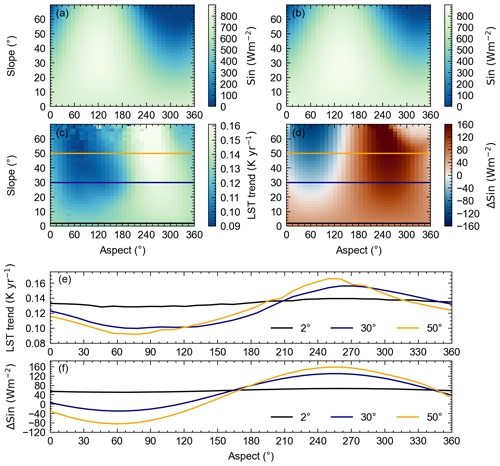
Figure 9Incoming shortwave radiation at 09:29 UTC (a) and 10:16 UTC (b), land surface temperature (LST) trend (c), and shortwave radiation difference between both times (ΔSin) (d) across Switzerland, excluding glaciers and all regions below 1700 m. Values are averaged for 2° slopes and 15° aspect bins. Cross sections of 30 and 50° slope angles show a similar sinusoidal pattern between the mean LST trend (e) and mean ΔSin (f), indicating LST trends biased by orbital drift.
4.1 Uncertainties related to LST and LST trends
Our comparison of Landsat-derived and in-situ-measured IMIS LSTs has shown good agreement with a mean accuracy of 0.26 K for the combined Landsat sensors (Fig. 4, Table 1). We observed no significant deviations in accuracy for the individual sensors, but the number of data points varies due to different temporal overlap of IMIS records and Landsat sensors. The slight positive bias of Landsat-derived LSTs greater than 0 °C compared to those measured from the IMIS stations is likely due to inaccurate IMIS LST data during snow-free conditions. The radiometric temperature measurements at the IMIS stations are based on a constant emissivity value of 0.98 for snow, resulting in biased temperatures in snow-free conditions. This explanation is consistent with greater accuracy at negative IMIS-derived LSTs, which are often associated with snow cover. The relatively large precision value of 4.69 K is likely in part due to the scatter around 0 °C, which is not necessarily a faulty or inaccurate measurement but rather caused by mixed-pixel effects due to the large resolution differences between IMIS and Landsat. During snowmelt periods, the IMIS sensor records ∼ 0 °C LST as long as snow persists under the sensor. Simultaneously, however, the larger footprint (60–120 m) of the Landsat measurement may record a mixed signal in the wider area around the IMIS station, potentially ranging from snow-free patches in sun-exposed areas to non-melting snow cover in shadows, for example. By excluding data points where IMIS LST is between −3.5 and +3.5 °C, which are 30% of all data points, the precision and uncertainty for L578 reduce to 4.37 and 4.38, respectively. Despite the relatively large uncertainty and a slight warm temperature bias, we find that the comparison of almost 4.5 × 10⁴ LST measurements shows good agreement. We note, however, that the IMIS network's spatial distribution does not fully represent the topographic complexity encountered in high mountains, as the stations are mostly installed on flat to gently sloping surfaces below 3000 m elevation.
The robustness of LST trends varies among Landsat sensors due to different temporal overlaps with the IMIS station data (Fig. 2). Using LST data from all three sensors, the temporal overlap with IMIS LST data covers a record length of 22.6 years. Trends with such large temporal overlap are aligned well around the 1:1 line with a mean accuracy of −0.02 K yr−1, while record lengths <15 years show significantly more variability. However, long record comparison is dominated by LE07, which has the most overlap in the observation period (Fig. 2). Although we are unable to evaluate LST trends from LT05 and LC08 based on long time series, our comparison together with the previous comparison of Landsat- and IMIS-derived LSTs for the different sensors provides confidence that LST trends derived from different Landsat sensors, spanning 38.5 years in total, are robust.
Besides the record length, the total number of LST observations also plays an important role in deriving robust LST trends. Although the Landsat archive covers 4 decades of LST observations, its temporal resolution of a 16 d revisit interval is rather low. In addition, cloud cover renders many scenes unusable, highlighting the need for reliable cloud masking. This raises two problems, especially for mountainous terrain. First, frequent cloud cover leads to inevitable data gaps, and, second, cloud detection algorithms are prone to failure over bright surfaces like snow and ice, which are common at high elevations. Our filter procedure, which is based on an initial LST model and thresholding the model–observation residuals in a second step, provides a way to detect unreasonably high or low LST values by taking the existing seasonal trend into account. We found that this filter more often removes unreasonably low LSTs, which are likely misclassified clouds, rather than high LSTs, potentially linked to wildfires. Yet, it is also possible that the Landsat cloud flag might have classified bright surfaces as clouds, resulting in the possible removal of valid LST observations. A robust and reliable cloud detection algorithm is currently the only practical way to minimize such problems.
The number of observations in the LST time series varies not only due to clouds, but also due to other systematic factors. Substantial spatial differences in LST counts arise from partial overlapping of adjacent Landsat paths (Fig. S3.1), which tends to increase towards the poles. In our study area, these overlaps yield approximately twice as many observations for a third of the area. Furthermore, the Landsat 7 scan line corrector failure further reduces data availability at smaller spatial scales. MALST, amplitude, and phase derived from LST time series seem to be generally unaffected by the variable number of observations as no large-scale patterns following the mentioned limitations can be observed (Fig. 6a, b, c). However, the LST trend is more sensitive to the number of observations, and subtle artifacts that align with the flight path of the satellite can be identified in some regions (Fig. 6d). In some regions faint stripes can be seen that correspond to the Landsat 7 scan line failure and thus reduced data availability. We assessed the robustness of LST trend calculations with respect to the number of observations through a systematic Monte Carlo simulation. By iteratively reducing the time series size (n=100) and performing repeated trend analyses (1000 repetitions), we quantified the impact of data reduction on trend stability. Each value of the 1000 repetitions was compared to the LST trend of the full time series (difference) and summarized as the mean and standard deviation. We chose the Landsat LST time series at the IMIS location of OFE2, comprising 1009 observations with an LST trend of 0.11 K yr−1, as an illustrative test site. The analysis revealed that although the mean LST trend value remains stable across sample sizes, the standard deviation, which represents the precision, varies more strongly. For common sample sizes of around 750 LST observations over the 38.5-year period, the 1σ value is 0.01.
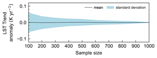
Figure 10Sensitivity analysis of land surface temperature (LST) trend stability. The LST trend anomaly shows the difference in the LST trend derived from the full time series and repeated LST trend calculations (1000 repetitions) with iteratively reduced sample sizes (n=100). Results are given as the mean and standard deviation.
4.2 Clear-sky bias
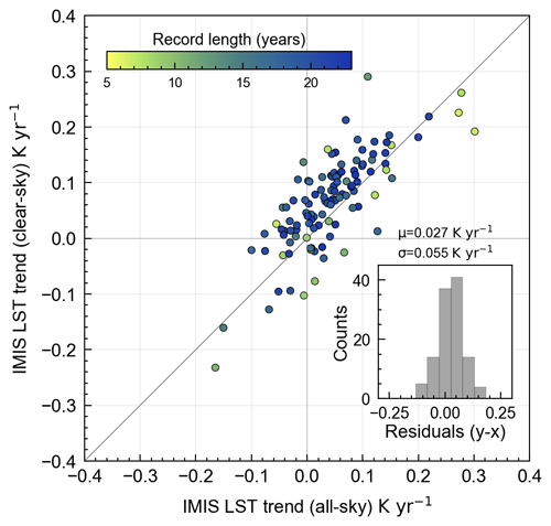
LST measurements based on thermal infrared remote sensing are biased towards clear-sky conditions (Ermida et al., 2019). The effect of such a bias on LST trends has not yet received much attention (Yang et al., 2024). A recent study has indicated no discernible impact of clear-sky bias on LST trends (Good et al., 2022) by comparing satellite-derived LST with 2 m air temperatures under clear-sky and all-sky conditions. Furthermore, Zhao et al. (2021) compared mean annual LST trends with trends in the frequency of clear-sky days and found no clear correlation for daytime LST but emphasized the challenges arising from changing surface conditions in the analysis. The Landsat data provide us with the timing of cloud cover and thus allow us to estimate the impact of cloud cover on LST trends at the IMIS locations. We compared IMIS LST trends derived during Landsat overpass days on clear-sky days with IMIS LST trends derived during all Landsat overpass times, including in clear-sky and cloudy-sky conditions. We found that on average LST trends during clear-sky conditions are 0.027 K yr−1 warmer than during all-weather conditions (Fig. 11). We note however that the spread in the data is relatively large, and we are reluctant to generalize this finding. Nevertheless, this exercise suggests that for our study area, an additional uncertainty of ∼ 0.03 K yr−1 is added for comparison between clear-sky and all-weather conditions.
4.3 LST trend bias due to changing acquisition times
Our analysis of changes in IMIS LST at 09:29 and 10:16 UTC (Fig. 8) and the spatial patterns of Landsat-derived LST trends with slope and aspect (Fig. 9) suggests the existence of an LST trend bias due to changing acquisition times. A linear fit of the acquisition times of all three sensors together does obviously not cover all the individual variations in orbit positions. However, the close similarity of the slope and aspect dependency in LST trends and ΔSin suggests that this approach appears to recover the first-order bias reasonably well. The dominant process that influences diurnal variations in LST during clear-sky conditions is the incoming solar radiation (Ghausi et al., 2023). Surfaces that are exposed to direct solar radiation receive particularly high amounts of energy and are thus prone to heating up quickly during the morning hours, especially during the summer months. The additional radiation flux received during the 47 min time window peaks for surfaces that are oriented orthogonal to the sun position, at an aspect value of approximately 130°, whereas the LST trend and ΔSin peak at approximately 255° (Fig. 9). Instead, our results suggest that the spatial pattern in the LST trend is more strongly controlled by the relative changes in direct solar radiation (ΔSin) during the 47 min time window rather than the total amount of energy received, with positive and negative peaks at approximately westerly- and easterly-exposed surfaces, respectively. As a result, the greatest temperature changes occur where surfaces have an orientation that results in a switch between sun exposure and shadow during the 47 min time window. Observed differences in the slope–aspect dependence of ΔSin and LST trends (Fig. 9a, b) are probably related to actual LST trends that are unrelated to slope and aspect.

Figure 12Mean LST trends (a), modeled LST trend bias (b), and corrected mean LST trends (c) for 2° slope and 10° aspect angles.
Possibly the simplest way to deal with the LST trend bias due to changing acquisition times would be to choose an observation time period in which the orbital drift was minimal, such as 1998–2018, or by neglecting Landsat 5 data altogether and Landsat 7 after 2018 (Fig. 2). We tested this shorter time period (Figs. S3.2, S3.3) and obtained LST trend values that were considerably noisier and more strongly affected by artifacts, seemingly related to the number of observations (see Sect. 4.1). We attribute this lower signal-to-noise ratio to the shorter observation time period, which also happened to be a limiting factor in our comparison with IMIS-derived trend values (Fig. 5). Previous studies concerned with the removal of the influence of orbital satellite drift on LST data – mostly for NOAA-AVHRR – have employed different techniques (e.g., Julien and Sobrino, 2012) that are, however, difficult to implement for Landsat due to substantially fewer observations and more heterogeneous terrain. In addition, correcting each observation to a consistent time before fitting Eq. (2) is prone to unquantified errors and spurious trends (Julien and Sobrino, 2012) and difficult to implement in GEE. We thus tested another possible approach, which is to estimate the LST trend bias after the fitting, based on the strong observed terrain influence (Fig. 9). This approach is probably less accurate as it neglects potential influences of different ground surface materials, but it is easier to implement.
To do so, we first smoothed the map of mean ΔSin for slope and aspect using local linear regression and normalized the values by the standard score. We then scaled the normalized model to approximate the observed LST trend pattern as a function of slope and aspect by least squares regression. Finally, we used the mean amount of surface warming (0.04 K yr−1) within the 47 min time window for flat and gently sloping terrain from the IMIS stations (Fig. 8) to align the model data for slope angles less than 10° (Fig. 12).
The modeled LST trend bias ranges between approximately 0 and 0.07 K yr−1, depending on slope and aspect. After removing the estimated bias, the remaining LST trends (Fig. 12c) still show some residual pattern that follows the topography, with about 0.02 K yr−1 lower trend values centered on a ∼ 160° aspect and ∼ 35° slope. The slope–aspect position of this residual LST trend feature is similar to the position of the highest Sin values in Fig. 9a and b. If there was an additional influence of the additional Sin, received during the 47 min time period, we would expect LST trend values to be higher on surfaces approximately orthogonal to the sun vector, not lower, as suggested by the observations. Therefore, it presently remains unclear whether the residual LST trend feature is due to the LST trend bias and an inadequate correction or possibly related to other processes. Applying the LST trend bias correction to the LST trends derived from GEE (Fig. 13) results in overall lower trend values and less spatial differences in LST trends with respect to aspect. Further spatial variations that are still present after the bias correction appear to be related to differences and changes in land cover types and warrant further detailed inspection. LST trends related to changes in the mountain cryosphere are discussed in Sect. 4.4, but a detailed analysis of land cover changes is beyond the scope of this study.
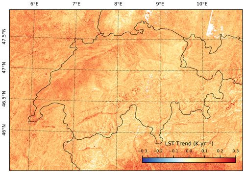
Figure 13Corrected land surface temperature (LST) trends of the Swiss Alps. Significance was estimated using a t test, and only significant (p<0.05) LST trends are shown in the map.

Figure 14Changes in the Unteraar Glacier, Switzerland, evidenced by late summer Landsat scenes from (a) 1984 and (b) 2022 and by (c) land surface temperature (LST) trends. The satellite images show false color composites using the shortwave infrared 1, near infrared, and red bands as red, green, and blue channels. The blue line in all panels indicates the outline of the Unteraar Glacier based on the Randolph Glacier Inventory (RGI Consortium, 2017).
4.4 Prospects for studying changes in the cryosphere
Based on the corrected LST trend map (Fig. 13), the spatially averaged (±1σ) Landsat-derived clear-sky LST trend for all of Switzerland and for the time period 1984–2022 is 0.1 ± 0.05 K yr−1. Insignificant (p>0.05) LST trends, determined by a t test, were masked out and not considered. Most LST trend values range from 0.07 to 0.09 K yr−1, with higher trends in populated valley bottoms like the Rhône Valley and lower trends over vegetated hillslopes at higher elevations (Fig. 7). A detailed analysis of LST trend variations with respect to different land cover types and properties as well as their change is beyond the scope of this study. However, we here briefly present examples of how changes in the mountain cryosphere map into spatial patterns of LST trends at high spatial resolution. For instance, the rapid changes in mountain glaciers correlate well with patterns observed in the LST trends. Figure 14 shows the Unteraar Glacier as an example, where the highest LST trends by far occur along the glacier margin due to ice retreat and exposure of bedrock. Additionally, high LST trends are associated with the expansion of supraglacial debris, which is well shown on the southern branch of the Unteraar Glacier, and the disappearance of clean ice in the lower few kilometers of the glacier. In contrast, LST trends are lower in magnitude and spatially more homogenous in the accumulation zone, which experiences minimal changes in surface type.
How changes in snow cover influence LST trends would require a detailed analysis with respect to snow extent, duration, depth, and seasonality, which is beyond the scope of this study. However, in order to assess the first-order sensitivity of LST trends to potential changes in snow cover, we spatially averaged LST trends for 100 m elevation bins and 1 °C MALST bins across the study area (Fig. 1), excluding glaciers and glacier retreat zones (see Sect. 2.4). Based on a previous global-scale study of air temperatures, we expect the highest positive temperature trends at altitudes where the MALST is between −10 and +5 °C due to reduced snow cover and increased absorption of solar radiation (Pepin and Lundquist, 2008). Observed mean LST trends at elevations where MALST is between −10 and 0 °C are among the highest trend values, consistent with an influence of snow cover on LST trends (Fig. 15). In fact, LST trend magnitudes display a systematic pattern with MALST and elevation that merits more detailed examination. We note that MALST differences of up to ∼ 20 K at a similar elevation are easily explained by different aspects, that is, exposure to the sun (see Fig. 7a), which may coincide with different long-term trends in snow cover duration. Although dominantly negative mean annual snow depth trends, derived from the IMIS stations by linear regression of annual mean snow depths, further support the effect of snow decline on LST trends, we did not find a clear correlation between LST trends and mean annual snow depth trends (Fig. 14b). In addition, we do observe mostly positive trends in the number of snow-free days per year (Fig. 15c), and these trends appear to increase in elevation. It is reasonable to assume that LST trends are higher where changes in snow cover are associated with more snow-free days and that LST trends are likely smaller where snow depth declines, but the surface nevertheless remains mostly snow covered, similar to that in glacier accumulation zones. However, a clear correlation between trends in the number of snow-free days and LST is not obvious, which could be related to the rather short record length of the IMIS stations and significant year-to-year variability in snow depth and cover.
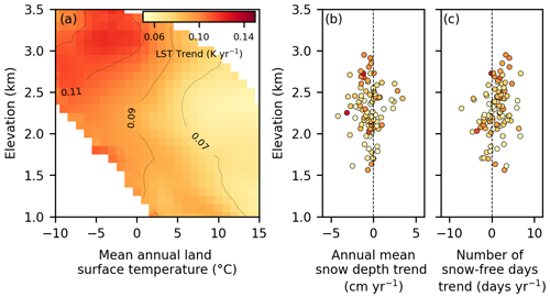
Figure 15Relationship between (a) mean land surface temperature (LST) trends for 100 m elevation bins and 1 °C mean annual land surface temperature (MALST) bins, (b) annual mean snow depth trends, and (c) trends in the number of annual snow-free days at the IMIS stations with a record length of more than 10 years.
Our study has shown that Landsat-derived land surface temperature (LST) data since 1984 offer opportunities to study the spatial variability of LST in complex topography at high spatial resolution. Our comparison with ground observations from the IMIS network provides confidence in the remote-sensing-derived LST data and LST trends, despite challenges due to differences in spatial resolution. The analysis of Landsat C2 LST time series, using harmonic regression including a linear component, exploits the periodic nature of the intra-annual LST variation and yields maps of the mean annual LST (MALST), the annual amplitude, the timing of the harmonic oscillation (phase), and the long-term LST trend. We observe meaningful spatial patterns with elevation, slope, and aspect that allow for the identification of the influence of surface orientation or type (e.g., glacier surfaces) on annual LST variations. However, all LST time series components (i.e., MALST, amplitude, phase, trend) presented in this study are based on LST at around ∼ 10:00 UTC, i.e., ∼ 11:00 local time, and must thus be interpreted accordingly. In principle, the Landsat archive provides a sufficiently long time series to obtain LST trends, as shown from our comparison with IMIS LST data. LST trend values obtained from Landsat and the IMIS network converge for record lengths >15 years, whereas shorter records exhibit considerably more noise. However, our analysis of the slope–aspect dependence of LST trends strongly suggests that trend values are biased due to the long-term orbit changes that cause spurious LST trends. As orbit variations are not uniform with time and the sensor, a temporal coherence correction is challenging. Assuming a long-term linear change in acquisition time, we have shown that the change in incident solar radiation can explain, at least in large part, the spatial slope–aspect patterns of “apparent” Landsat-derived LST trends. By modeling and removing the LST trend bias due to changing acquisition time, we obtain a spatially averaged (±1σ) Landsat-derived clear-sky LST trend for the time period 1984–2022 of 0.1 ± 0.05 K yr−1. The corrected LST trends respond to changes in the mountain cryosphere, such as glacier retreat, debris cover evolution, and snow decline, and can potentially contribute to an improved prediction of permafrost temperatures, as surface temperatures propagate into greater depths. Further analysis is needed to disentangle the effect of land cover and land cover changes on the observed LST trends.
GeoTIFF files of the mean annual land surface temperature, amplitude, land surface temperature trend, RMSE, and phase of the harmonic oscillation, together with the Google Earth Engine Python code, are available from the repository at https://doi.org/10.5880/GFZ.3.3.2023.005 (Gök et al., 2024).
The supplement related to this article is available online at: https://doi.org/10.5194/tc-18-5259-2024-supplement.
DTG: conceptualization, methodology, writing (original draft and review and editing). DS: conceptualization, methodology, writing (review and editing), supervision. HW: methodology, writing (review and editing).
The contact author has declared that none of the authors has any competing interests.
Publisher’s note: Copernicus Publications remains neutral with regard to jurisdictional claims made in the text, published maps, institutional affiliations, or any other geographical representation in this paper. While Copernicus Publications makes every effort to include appropriate place names, the final responsibility lies with the authors.
We are grateful to Noel Gorelick for advice regarding Google Earth Engine. During the preparation of this work, the authors checked spelling and grammar using DeepL and ChatGPT to improve readability. After using these tools, the authors reviewed and edited the content and take full responsibility for the content of the publication.
This research has been supported by the European Research Council under the EU H2020 program (grant no. 759639).
The article processing charges for this open-access publication were covered by the Helmholtz Centre Potsdam – GFZ German Research Centre for Geosciences.
This paper was edited by Franziska Koch and reviewed by two anonymous referees.
Allen, S., Gruber, S., and Owens, I. F.: Exploring steep bedrock permafrost and its relationship with recent slope failures in the Southern Alps of New Zealand, Permafrost Periglac., 20, 345–356, https://doi.org/10.1002/ppp.658, 2009.
Bojinski, S., Verstraete, M. M., Peterson, T. C., Richter, C., Simmons, A. J., and Zemp, M.: The concept of essential climate variables in support of climate research, applications, and policy, B. Am. Meteorol. Soc., 95, 1431–1443, https://doi.org/10.1175/bams-d-13-00047.1, 2014.
Brantley, S. L., Goldhaber, M. B., and Ragnarsdottir, K.: Crossing disciplines and scales to understand the critical zone, Elements, 3, 307–314, https://doi.org/10.2113/gselements.3.5.307, 2007.
Cook, M., Schott, J. R., Mandel, J., and Raqueño, N. G.: Development of an Operational Calibration Methodology for the Landsat Thermal Data Archive and Initial Testing of the Atmospheric Compensation Component of a Land Surface Temperature (LST) Product from the Archive, Remote Sensing, 6, 11244–11266, https://doi.org/10.3390/rs61111244, 2014.
Copernicus DEM: COP-DEM_EEA-10-INSP, Copernicus DEM [data set], https://doi.org/10.5270/esa-c5d3d65, 2022.
Corripio, J. G.: Vectorial algebra algorithms for calculating terrain parameters from DEMs and solar radiation modelling in mountainous terrain, Int. J. Geogr. Inf. Sci., 17, 1–23, https://doi.org/10.1080/713811744, 2003.
Crawford, C. J., Roy, D. P., Arab, S., Barnes, C., Vermote, É., Hulley, G., Gerace, A., Choate, M. J., Engebretson, C., Micijevic, E., Schmidt, G. L., Anderson, C., Anderson, M. C., Bouchard, M., Cook, B. D., Dittmeier, R., Howard, D. M., Jenkerson, C. B., Kim, M., Kleynhans, T., Maiersperger, T., Mueller, C., Neigh, C. S. R., Owen, L. R., Page, B. P., Pahlevan, N., Rengarajan, R., Roger, J. C., Sayler, K. L., Scaramuzza, P., Skakun, S., Yan, L., Zhang, H. K., Zhu, Z., and Zahn, S.: The 50-year Landsat collection 2 archive, Science of Remote Sensing, 8, 100103, https://doi.org/10.1016/j.srs.2023.100103, 2023.
Dech, S., Holzwarth, S., Asam, S., Andresen, T., Bachmann, M., Boettcher, M., Dietz, A. J., Eisfelder, C., Frey, C., Gesell, G., Geßner, U., Hirner, A., Hofmann, M., Kirches, G., Klein, D., Klein, I., Kraus, T., Krause, D., Plank, S., Popp, T., Reinermann, S., Reiners, P., Roessler, S., Ruppert, T., Scherbachenko, A., Vignesh, R., Wolfmueller, M., Zwenzner, H., and Kuenzer, C.: Potential and Challenges of Harmonizing 40 years of AVHRR Data: The TIMELINE Experience, Remote Sensing, 13, 3618, https://doi.org/10.3390/rs13183618, 2021.
Dwyer, J. L., Roy, D. P., Sauer, B., Jenkerson, C. B., Zhang, H. K., and Lymburner, L.: Analysis Ready Data: Enabling analysis of the Landsat Archive, Remote Sensing, 10, 1363, https://doi.org/10.3390/rs10091363, 2018.
Ermida, S. L., Trigo, I. F., DaCamara, C. C., Jiménez, C., and Prigent, C.: Quantifying the Clear-Sky bias of satellite land surface temperature using Microwave-Based estimates, J. Geophys. Res.-Atmos., 124, 844–857, https://doi.org/10.1029/2018jd029354, 2019.
Foga, S., Scaramuzza, P., Guo, S., Zhu, Z., Dilley, R. D., Beckmann, T., Schmidt, G. L., Dwyer, J. L., Hughes, M. J., and Laue, B.: Cloud detection algorithm comparison and validation for operational Landsat data products, Remote Sens. Environ., 194, 379–390, https://doi.org/10.1016/j.rse.2017.03.026, 2017.
Fu, P. and Weng, Q.: Temporal dynamics of land surface temperature from Landsat TIR Time Series images, IEEE Geosci. Remote S., 12, 2175–2179, https://doi.org/10.1109/lgrs.2015.2455019, 2015.
Ghausi, S. A., Tian, Y., Zehe, E., and Kleidon, A.: Radiative controls by clouds and thermodynamics shape surface temperatures and turbulent fluxes over land, P. Natl. Acad. Sci. USA, 120, e2220400120, https://doi.org/10.1073/pnas.2220400120, 2023.
Gök, D. T., Scherler, D., and Wulf, H.: Landsat-derived spatiotemporal variations of land surface temperature, GFZ Data Services [data set], https://doi.org/10.5880/GFZ.3.3.2023.005, 2024.
Good, E., Aldred, F., Jimenez, C., Veal, K. L., and Jiménez, C.: An Analysis of the Stability and Trends in the LST_ cci Land Surface Temperature Datasets Over Europe, Earth and Space Science, 9, e2022EA002317, https://doi.org/10.1029/2022ea002317, 2022.
Gruber, S. and Haeberli, W.: Permafrost in steep bedrock slopes and its temperature-related destabilization following climate change, J. Geophys. Res., 112, F02S18, https://doi.org/10.1029/2006jf000547, 2007.
Gruber, S., Hoelzle, M., and Haeberli, W.: Permafrost thaw and destabilization of Alpine rock walls in the hot summer of 2003, Geophys. Res. Lett., 31, L13504, https://doi.org/10.1029/2004gl020051, 2004.
Guillevic, P., Göttsche, F.-M., Nickeson, J., Hulley, G., Ghent, D., Yu, Y., Trigo, I. F., Hook, S. J., Sobrino, J. A., Remedios, J. J., Román, M. O., and Camacho, F.: Land Surface Temperature Product Validation Best Practice Protocol Version 1.0, Land Product Validation Subgroup (WGCV/CEOS), NASA [data set], https://doi.org/10.5067/doc/ceoswgcv/lpv/lst.001, 2017.
Gutman, G. E.: On the use of long-term global data of land reflectances and vegetation indices derived from the advanced very high resolution radiometer, J. Geophys. Res., 104, 6241–6255, https://doi.org/10.1029/1998jd200106, 1999.
Gutman, G. E. and Masek, J.: Long-term time series of the Earth's land-surface observations from space, Int. J. Remote Sens., 33, 4700–4719, https://doi.org/10.1080/01431161.2011.638341, 2012.
Harris, C., Arenson, L. U., Christiansen, H. H., Etzelmüller, B., Frauenfelder, R., Gruber, S., Haeberli, W., Hauck, C., Hölzle, M., Humlum, O., Isaksen, K., Kääb, A., Kern-Lütschg, M. A., Lehning, M., Matsuoka, N., Murton, J. B., Noetzli, J., Phillips, M., Ross, N., Seppälä, M., Springman, S. M., and Mühll, D. V.: Permafrost and climate in Europe: Monitoring and modelling thermal, geomorphological and geotechnical responses, Earth-Sci. Rev., 92, 117–171, https://doi.org/10.1016/j.earscirev.2008.12.002, 2009.
Huggel, C.: Recent extreme slope failures in glacial environments: effects of thermal perturbation, Quaternary Sci. Rev., 28, 1119–1130, https://doi.org/10.1016/j.quascirev.2008.06.007, 2009.
Hulley, G. and Hook, S. J.: Generating consistent land surface temperature and emissivity products between ASTER and MODIS data for earth science research, IEEE T. Geosci. Remote, 49, 1304–1315, https://doi.org/10.1109/tgrs.2010.2063034, 2011.
Hulley, G., Hook, S. J., Abbott, E. A., Malakar, N. K., Islam, T., and Abrams, M. J.: The ASTER Global Emissivity Dataset (ASTER GED): Mapping Earth's emissivity at 100 meter spatial scale, Geophys. Res. Lett., 42, 7966–7976, https://doi.org/10.1002/2015gl065564, 2015.
Hulley, G., Ghent, D., Göttsche, F.-M., Guillevic, P., Mildrexler, D. J., and Coll, C.: Land surface temperature, in: Elsevier eBooks, 57–127, https://doi.org/10.1016/b978-0-12-814458-9.00003-4, 2019.
IPCC: Climate Change 2023: Synthesis Report: Contribution of Working Groups I, II and III to the Sixth Assessment Report of the Intergovernmental Panel on Climate Change, edited by: Core Writing Team, Lee, H., and Romero, J., IPCC, Geneva, Switzerland, https://doi.org/10.59327/IPCC/AR6-9789291691647, 2023
Jiménez-Muñoz, J. C. and Sobrino, J. A.: A generalized single-channel method for retrieving land surface temperature from remote sensing data, J. Geophys. Res., 108, 4688, https://doi.org/10.1029/2003jd003480, 2003.
Jin, M. and Treadon, R.: Correcting the orbit drift effect on AVHRR land surface skin temperature measurements, Int. J. Remote Sens., 24, 4543–4558, https://doi.org/10.1080/0143116031000095943, 2003.
Julien, Y. and Sobrino, J. A.: Correcting AVHRR Long Term Data Record V3 estimated LST from orbital drift effects, Remote Sens. Environ., 123, 207–219, https://doi.org/10.1016/j.rse.2012.03.016, 2012.
Julien, Y. and Sobrino, J. A.: Toward a reliable correction of NOAA AVHRR orbital drift, Frontiers in Remote Sensing, 3, 851933, https://doi.org/10.3389/frsen.2022.851933, 2022.
Kalnay, E., Kanamitsu, M., Kistler, R., Collins, W. G., Deaven, D. G., Gandin, L. S., Iredell, M., Saha, S., White, G. H., Woollen, J. S., Zhu, Y., Chelliah, M., Ebisuzaki, W., Higgins, W., Janowiak, J. E., Mo, K. C., Ropelewski, C. F., Wang, J., Leetmaa, A., Reynolds, R. W., Jenne, R. L., and Joseph, D.: The NCEP/NCAR 40-Year Reanalysis Project, B. Am. Meteorol. Soc., 77, 437–471, https://doi.org/10.1175/1520-0477(1996)077<0437:TNYRP>2.0.CO;2, 1996.
Kennedy, R. E., Yang, Z., and Cohen, W. B.: Detecting trends in forest disturbance and recovery using yearly Landsat time series: 1. LandTrendr – Temporal segmentation algorithms, Remote Sens. Environ., 114, 2897–2910, https://doi.org/10.1016/j.rse.2010.07.008, 2010.
Kuenzer, C. and Dech, S.: Thermal Infrared Remote Sensing: Sensors, Methods, Applications, Springer Science & Business Media, https://doi.org/10.1007/978-94-007-6639-6, 2013.
Li, J., Li, Z.-L., Wu, H., and You, N.: Trend, seasonality, and abrupt change detection method for land surface temperature time-series analysis: Evaluation and improvement, Remote Sens. Environ., 280, 113222, https://doi.org/10.1016/j.rse.2022.113222, 2022.
Li, Z., Wu, H., Duan, S., Zhao, W., Ren, H., Li, X., Leng, P., Tang, R., Ye, X., Zhu, J., Sun, Y., Si, M., Liu, M., Li, J., Zhang, X., Shang, G., Tang, B., Yan, G., and Zhou, C.: Satellite Remote sensing of global land surface temperature: definition, methods, products, and applications, Rev. Geophys., 61, e2022RG000777, https://doi.org/10.1029/2022rg000777, 2023.
Li, Z.-L., Tang, B., Wu, H., Ren, H., Yan, G., Wan, Z., Trigo, I. F., and Sobrino, J. A.: Satellite-derived land surface temperature: Current status and perspectives, Remote Sens. Environ., 131, 14–37, https://doi.org/10.1016/j.rse.2012.12.008, 2013.
Malakar, N. K., Hulley, G., Hook, S. J., Laraby, K. G., Cook, M., and Schott, J. R.: An Operational Land Surface Temperature Product for Landsat Thermal Data: Methodology and Validation, IEEE T. Geosci. Remote, 56, 5717–5735, https://doi.org/10.1109/tgrs.2018.2824828, 2018.
Matiu, M., Crespi, A., Bertoldi, G., Carmagnola, C. M., Marty, C., Morin, S., Schöner, W., Cat Berro, D., Chiogna, G., De Gregorio, L., Kotlarski, S., Majone, B., Resch, G., Terzago, S., Valt, M., Beozzo, W., Cianfarra, P., Gouttevin, I., Marcolini, G., Notarnicola, C., Petitta, M., Scherrer, S. C., Strasser, U., Winkler, M., Zebisch, M., Cicogna, A., Cremonini, R., Debernardi, A., Faletto, M., Gaddo, M., Giovannini, L., Mercalli, L., Soubeyroux, J.-M., Sušnik, A., Trenti, A., Urbani, S., and Weilguni, V.: Observed snow depth trends in the European Alps: 1971 to 2019, The Cryosphere, 15, 1343–1382, https://doi.org/10.5194/tc-15-1343-2021, 2021.
Muro, J., Strauch, A., Heinemann, S., Steinbach, S., Thonfeld, F., Waske, B., and Diekkrüger, B.: Land surface temperature trends as indicator of land use changes in wetlands, Int. J. Appl. Earth Obs., 70, 62–71, https://doi.org/10.1016/j.jag.2018.02.002, 2018.
Pepin, N. and Lundquist, J. D.: Temperature trends at high elevations: Patterns across the globe, Geophys. Res. Lett., 35, L14701, https://doi.org/10.1029/2008gl034026, 2008.
Prata, A. J.: Land surface temperatures derived from the advanced very high resolution radiometer and the along-track scanning radiometer: 2. Experimental results and validation of AVHRR algorithms, J. Geophys. Res., 99, 13025–13058, https://doi.org/10.1029/94jd00409, 1994.
Qiu, S., Zhu, Z., Shang, R., and Crawford, C. J.: Can Landsat 7 preserve its science capability with a drifting orbit?, Science of Remote Sensing, 4, 100026, https://doi.org/10.1016/j.srs.2021.100026, 2021.
Reiners, P., Sobrino, J. A., and Kuenzer, C.: Satellite-Derived Land Surface Temperature Dynamics In the Context of Global Change – A Review, Remote Sensing, 15, 1857, https://doi.org/10.3390/rs15071857, 2023.
Ren, S., Yao, T., Yang, W., Miles, E., Zhao, H., Zhu, M., and Li, S.: Changes in glacier surface temperature across the Third Pole from 2000 to 2021, Remote Sens. Environ., 305, 114076, https://doi.org/10.1016/j.rse.2024.114076, 2024.
RGI Consortium: Randolph Glacier Inventory: A dataset of global glacier outlines (Version 6), National Snow and Ice Data Center [data set], https://doi.org/10.7265/4m1f-gd79, 2017.
Roy, D. P., Li, Z., Zhang, H. K., and Huang, H.-C.: A conterminous United States analysis of the impact of Landsat 5 orbit drift on the temporal consistency of Landsat 5 Thematic Mapper data, Remote Sens. Environ., 240, 111701, https://doi.org/10.1016/j.rse.2020.111701, 2020.
Rumpf, S. B., Gravey, M., Broennimann, O., Luoto, M., Cianfrani, C., Mariéthoz, G., and Guisan, A.: From white to green: Snow cover loss and increased vegetation productivity in the European Alps, Science, 376, 1119–1122, https://doi.org/10.1126/science.abn6697, 2022.
Shumway, R. H. and Stoffer, D. S.: Time Series Analysis and its applications: With R Examples, third edition, 3rd edn., Int. Stat. Rev., 81, 323–325, https://doi.org/10.1111/insr.12020_15, 2013.
Smith, S. L., O'Neill, H. B., Isaksen, K., Noetzli, J., and Romanovsky, V. E.: The changing thermal state of permafrost, Nature Reviews Earth & Environment, 3, 10–23, https://doi.org/10.1038/s43017-021-00240-1, 2022.
Sobrino, J. A., Julien, Y., and García-Monteiro, S.: Surface Temperature of the Planet Earth from Satellite Data, Remote Sensing, 12, 218, https://doi.org/10.3390/rs12020218, 2020.
Walter, F., Amann, F., Kos, A., Kenner, R., Phillips, M., De Preux, A., Huss, M., Tognacca, C., Clinton, J., Diehl, T., and Bonanomi, Y.: Direct observations of a three million cubic meter rock-slope collapse with almost immediate initiation of ensuing debris flows, Geomorphology, 351, 106933, https://doi.org/10.1016/j.geomorph.2019.106933, 2020.
Weng, Q. and Fu, P.: Modeling annual parameters of clear-sky land surface temperature variations and evaluating the impact of cloud cover using time series of Landsat TIR data, Remote Sens. Environ., 140, 267–278, https://doi.org/10.1016/j.rse.2013.09.002, 2014.
Yang, Y., Zhao, W., Yang, Y., Xu, M., Mukhtar, H., Tauqir, G., and Tarolli, P.: An annual temperature cycle feature constrained method for generating MODIS daytime All-Weather land surface temperature, IEEE T. Geosci. Remote, 62, 4405014, https://doi.org/10.1109/tgrs.2024.3377670, 2024.
Zhang, H. K. and Roy, D. P.: Landsat 5 Thematic Mapper reflectance and NDVI 27-year time series inconsistencies due to satellite orbit change, Remote Sens. Environ., 186, 217–233, https://doi.org/10.1016/j.rse.2016.08.022, 2016.
Zhao, W., Yang, M., Chang, R., Zhan, Q., and Li, Z.-L.: Surface warming trend analysis based on MODIS/Terra Land surface temperature product at Gongga Mountain in the southeastern Tibetan Plateau, J. Geophys. Res.-Atmos., 126, https://doi.org/10.1029/2020jd034205, 2021.
Zhu, Z. and Woodcock, C. E.: Object-based cloud and cloud shadow detection in Landsat imagery, Remote Sens. Environ., 118, 83–94, https://doi.org/10.1016/j.rse.2011.10.028, 2012.


