A simple snow temperature index model exposes discrepancies between reanalysis snow water equivalent products

Current global reanalyses show marked discrepancies in snow mass and snow cover extent for the Northern Hemisphere. Here, benchmark snow datasets are produced by driving a simple offline snow model, the Brown Temperature Index Model (B-TIM), with temperature and precipitation from three reanalyses. The B-TIM offline snow performs comparably to or better than online (coupled land–atmosphere) reanalysis snow when evaluated against in situ snow measurements. Sources of discrepancy in snow climatologies, which are difficult to isolate when comparing online reanalysis snow products amongst themselves, are partially elucidated by separately bias-adjusting temperature and precipitation in the B-TIM. Interannual variability in snow mass and snow spatial patterns is far more self-consistent amongst offline B-TIM snow products than amongst online reanalysis snow products, and the self-consistent products are more similar to in situ observations, as evaluated in a validation study. Specific artifacts related to temporal inhomogeneity in snow data assimilation are revealed in the analysis. The B-TIM, released here as an open-source, self-contained Python package, provides a simple benchmarking tool for future updates to more sophisticated online and offline snow datasets.

1 Introduction

Terrestrial snow is a highly variable component of the cryosphere that responds to and feeds back on anthropogenic global warming via snow albedo (e.g., Betts et al., 2014; Thackeray et al., 2018). At its maximum, snow covers up to 50 % of the Northern Hemisphere land surface (Robinson and Frei, 2000), and it controls a wide range of hydrological, ecological, and socio-economic systems (Bokhorst et al., 2016). Snow variability and trends have been monitored over several decades (Doesken and Judson, 1997; Mudryk et al., 2020; Robinson, 1989) with regular reporting, such as in the annual National Oceanic and Atmospheric Administration (NOAA) Arctic Report Card. Despite this attention to snow, there are marked discrepancies in historical snow estimates from available products, leading to gaps in our understanding of snow across a range of spatial scales, from point to watershed to hemispheric (Magnusson et al., 2015; Mudryk et al., 2015). Many factors lead to these discrepancies, making it a challenge to identify a single authoritative dataset for historical snow water equivalent or related variables. Furthermore, the simplest snow models can perform comparably to the most complex snow models in relation to the available in situ observations (Boone and Etchevers, 2001; Essery et al., 2013; Magnusson et al., 2015; Menard et al., 2021). For this reason, “offline” datasets generated with temperature index models (TIMs), snow models forced only by air temperature and precipitation that do not represent coupling of snow to the land–atmosphere system, are still maintained (e.g., Hock, 2003; Ohmura, 2001; Sturm, 2015; Walter et al., 2005). Recent studies have advocated for the use of multi-product ensembles spanning a range of complexities (including offline snow models, land surface data assimilation systems, and coupled atmosphere–land reanalysis systems) and a range of snow schemes from single-layer to multilayer snow modules embedded inside comprehensive land surface models. These ensembles can then be used to characterize snow climatology and trends (e.g., Mudryk et al., 2024), evaluate new snow datasets, or quantify uncertainties (Essery, 2015; Kim et al., 2021; Mudryk et al., 2015). Methods to evaluate the quality of potential ensemble members are actively being explored.

In this study, we use an offline TIM to investigate the discrepancies in snow water equivalent (SWE) and snow cover extent (SCE) in online reanalysis snow products. We use an updated version of the Brown et al. (2003) TIM, hereafter called the B-TIM (Brown Temperature Index Model), whose broad applicability and extensive legacy at Environment and Climate Change Canada (ECCC) motivate its use. The model was initially developed to provide a first-guess field for a gridded snow analysis using forcing from the European Centre for Medium-range Weather Forecasts (ECMWF) Reanalysis 15 (ERA-15). The snow analysis was used to evaluate global climate model output from AMIP II. Later, using forcing from numerical weather forecasts to run the B-TIM, the model was incorporated into the Canadian Meteorological Centre's (CMC's) daily snow depth analysis (Brown and Brasnett, 2010). This dataset continues to be used as a validation product for other studies (Kim et al., 2021; Zhang et al., 2014). Until recently, the standalone version of the B-TIM that is internally available at ECCC was coded in Fortran 77 and forced with temperature and precipitation forcing from ERA-Interim (Dee et al., 2011). The ERA-Interim version participated in several ensemble studies (e.g., Brown et al., 2010; Brown and Robinson, 2011; Mortimer et al., 2020) and provided hemispheric snow mass estimates for the NOAA Arctic Report Card (2017 edition to 2020 edition; e.g., Mudryk et al., 2020) but has been superseded by a version forced with ERA5. In addition to updated forcing, following ECCC's push to provide transparent and reproducible open-source climate assessment tools based on FAIR (findable, accessible, interoperable, and reusable) principles (Environment and Climate Change Canada, 2021), we are motivated to release the B-TIM as an open-source code following updated coding standards.

Discrepancies in snow from “online” coupled reanalyses arise from many sources, including inconsistencies in terms of snow data assimilation schemes, underlying snow and land–surface component model differences, atmospheric model differences, differences in processes governing the coupled surface energy balance, and interactions between all these factors. To highlight one example which we will discuss in more detail below, while the assimilation of snow data may improve instantaneous estimates of snow depth, there is evidence that significant time series discontinuities may result as contributions to the data stream change (as in ERA5; Mortimer et al., 2020). Like any offline TIM, the B-TIM does not assimilate snow data, does not capture surface energetics, and features no coupling between snow and the land–atmosphere state. The B-TIM offline snow products, provided they are suitably validated, can thus isolate the role of meteorological driving from issues related to data assimilation, model bias, and errors arising from coupling, all of which can be sources of discrepancy for more sophisticated snow datasets. In this work, we use a fixed version of the B-TIM without further calibration or tuning. Therefore, one parameter set for the model is used, and the results may still contain model bias. Quantifying this bias for the B-TIM can be done through the analysis of parameter and error sensitivity (Essery, 2015; Raleigh et al., 2015). However, our aim is to investigate reanalysis snow biases; each offline snow product will have the same model bias, whereas the coupled reanalysis snow does not. Comparing offline snow products therefore narrows down the sources of discrepancy without requiring a re-run of the complex snow modelling and data assimilation process.

We document an updated B-TIM algorithm (Sect. 2), which we release here as an open-source, self-contained Python repository. We then use the B-TIM to generate offline SWE and snow cover extent using temperature and precipitation forcing from the global reanalyses ERA5, JRA-55, and MERRA-2 for 1980–2020. Through validation with in situ data, we compare the realism of the offline B-TIM and online coupled reanalyses (Sect. 3). This study has as its focus hemispheric snow. Even at these large scales and excluding complexities tied to mountain snow modelling, there are discrepancies that should be characterized. For exploration into regional performance, two other studies have been prepared for publication: Mudryk et al. (2024) and Mortimer et al. (2024). These include all the datasets discussed here. Mudryk et al. (2024) evaluate a suite of 23 gridded SWE products, ranking them by performance and inter-dataset consistency. Mortimer et al. (2024) present an expanded reference SWE dataset that combines in situ and airborne SWE measurement and assess snow dataset performance against that record. The same in situ data are used for this study. Our main scientific work here, which is described in Sect. 3, will be to use the B-TIM to characterize and explain discrepancies amongst online reanalysis snow products' climatological characteristics and interannual variabilities. This analysis will include the use of bias-adjusted temperature and precipitation forcing in the B-TIM to elucidate sources of discrepancy. We discuss results and conclusions in Sect. 4.

2 Data and methods

2.1 The B-TIM snow model

The calculations described in this section, which can also be seen in the schematic in Fig. 1, comprise version 1.0.0 of the B-TIM (https://doi.org/10.5281/zenodo.10044950; Elias Chereque et al., 2024). This is the first updated description in this model's 2 decades of usage in many publications and applications. Relative to Brown et al. (2003), we provide updated documentation and changes to some constants, as reflected in the code and its parameters. Physical constants and parameter values can be found in Table S1 in the Supplement. At a given time step, we denote the initial snow depth and density by D_i and ρ_i. SWE_i is the initial time step's snow water equivalent, calculated as SWE_i= ρ_iD_i (with units of kg m⁻²). All densities have standard units (kg m⁻³), and snow depths have units of metres.

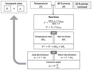
Figure 1 Conceptual overview of the Brown Temperature Index Model (B-TIM). At every time step and location, temperature and precipitation values are used to compute either the density and depth of any new snow or the temperature of any rainfall. The snowpack state (snow depth and density) is affected by rain melt, melting due to air temperature, and one of two densification processes which cause both depth and density variables to evolve.

2.1.1 Initialization, meteorological driving, and time stepping

Each simulated snow year is initialized from snow-free conditions on 1 August and runs until the following 31 July; 2 m temperature and total precipitation (frozen and solid) are the only inputs to the model. The specific variables we used from each reanalysis are listed in Table S2. A fixed 20 % precipitation reduction is implemented at each model time step as a general loss parameter – this captures canopy interception, sublimation, and blowing snow for frozen precipitation. The variable P represents the reduced precipitation in metres of water for a given time step and location. The model time step is 1 h, but less frequent driving data can be handled. If needed, the model linearly interpolates temperature to hourly steps and divides accumulated precipitation by the duration of the driving-data time step in hours.

2.1.2 Determining precipitation phase

At each model time step, the precipitation phase is classified as snow or rain using a 0 °C threshold. Previous B-TIM applications allowed mixed precipitation between 0 and 2 °C following a linear relationship for the liquid fraction. For large-scale studies, there is little advantage to including mixed precipitation according to the linear relationship as opposed to a fixed threshold as both are coarse simplifications (Jennings and Molotch, 2019). The absence of mixed precipitation has a minimal impact on the aggregated variables, though it causes local differences in regions with ephemeral snow.

2.1.3 Updating snow depth and density

Following Hedstrom and Pomeroy (1998), frozen precipitation during a time step is assigned a “new-snow” density:

$$\begin{array}{}\text{(1)}& {\mathit{\rho }}_{\mathrm{new}}=A+{\mathrm{Be}}^{T/C}T<\mathrm{0}\mathrm{°}\mathrm{C},\end{array}$$

where T is the air temperature (values of the constants are listed in Table S1).

Intermediate values for snow depth and density are assigned to the model's single snow layer.

$$\begin{array}{}\text{(2a)}& {\displaystyle }{D}^{\ast }=D_{\mathrm{i}}+P\left({\displaystyle \frac{{\mathit{\rho }}_{\mathrm{w}}}{{\mathit{\rho }}_{\mathrm{new}}}}\right)\text{(2b)}& {\displaystyle }{\mathit{\rho }}^{\ast }={\displaystyle \frac{\left(D_{\mathrm{i}}{\mathit{\rho }}_{\mathrm{i}}+P{\mathit{\rho }}_{\mathrm{w}}\right)}{D^{\ast }}}\end{array}$$

Three densification or melting steps are then applied to evolve ρ^∗ and D^∗.

1. Snowmelt is computed at each model time step using a melt factor, γ (mm w.e. K⁻¹ h⁻¹), which is based on the intermediate snow layer density, ρ^∗. The relationship used to calculate γ is based on Kuusisto (1984):

   $$\begin{array}{}\text{(3)}& \mathit{\gamma }=M_{\mathrm{1}}{\mathit{\rho }}^{\ast }-M_{\mathrm{2}}.\end{array}$$

   Lower and upper bounds of $\mathrm{4.1}\times {\mathrm{10}}^{-\mathrm{3}}$ and 0.23, respectively, are enforced on γ. Hourly melt, represented as the change in snow depth ΔD_m, follows a standard temperature index approach:

   $$\begin{array}{}\text{(4)}& \mathrm{\Delta }{D}_{\mathrm{m}}=\left\{\begin{array}{l}-\frac{\left(T-T_{\mathrm{melt}}\right)}{{\mathit{\rho }}^{\ast }}\mathit{\gamma },T>T_{\mathrm{melt}}\\ \mathrm{0},T\le T_{\mathrm{melt}},\end{array}\right.\end{array}$$

   where $T_{\mathrm{melt}}=-\mathrm{1}$ °C is the threshold air temperature used for snowmelt.

   The leading coefficient in Eq. (3), M₁, has been halved relative to Brown et al. (2003) to reduce the rate of snowmelt during the ablation season. This has been implemented for the CMC snow product.

2. Snowmelt caused by rainfall on the snowpack is computed using

   $$\begin{array}{}\text{(5)}& \mathrm{\Delta }{D}_{\mathrm{r}}=-{\displaystyle \frac{R{\mathit{\rho }}_{\mathrm{w}}{C}_{\mathrm{w}}(T_{\mathrm{w}}-T_{\mathrm{freeze}})}{L_{\mathrm{f}}{\mathit{\rho }}^{\ast }}}.\end{array}$$

   C_w is the heat capacity of water (J kg⁻¹ K⁻¹), R is the total rainfall (m), T_w is the rainfall temperature (°C), ρ_w is the density of liquid water, and L_f is the latent heat of fusion for ice (J kg⁻¹). Rain temperature is taken to be equal to air temperature, as in Brown et al. (2003), and the snowpack is assumed to be isothermal and 0 °C, implying instant melting of the snowpack when it is warmed.

3. A second intermediate snow depth is computed based on these first two steps.

   $$\begin{array}{}\text{(6)}& D^{\ast \ast }=D^{\ast }+\mathrm{\Delta }{D}_{\mathrm{m}}+\mathrm{\Delta }{D}_{\mathrm{r}}\end{array}$$

   Depending on air temperature, one of two possible densification processes is implemented. Both processes initially affect density (Eqs. 7 and 9), and then snow depth is adjusted to conserve total water.

   Cold. When temperatures are below T_melt, cold-snow ageing is implemented as follows:

   $$\begin{array}{}\text{(7)}& \begin{array}{rl}\mathrm{\Delta }{\mathit{\rho }}_{\mathrm{c}}& ={\mathrm{C}}_{\mathrm{1}}\left({\mathrm{SWE}}^{\ast }\right)\exp \left[{\mathrm{C}}_{\mathrm{3}}\left(T_{\mathrm{melt}}-T_{\mathrm{snow}}\right)\right]\\ & \exp \left[-{\mathrm{C}}_{\mathrm{2}}{\mathit{\rho }}^{\ast }\right],T<T_{\mathrm{melt}}.\end{array}\end{array}$$

   SWE^∗ is the snow water equivalent (kg m⁻², calculated as the product ${\mathit{\rho }}^{\ast }{D}^{\ast \ast })$. C₁ and C₂ are empirically derived constants. This formulation was proposed in Anderson (1976), and the parameters used in the B-TIM are in the accepted range. T_snow is the snow temperature, taken to be equal to air temperature in this step. Snowpack density is allowed to vary between 200 and 550 kg m⁻³. The densification process does not vary seasonally.

   Warm. When temperatures are above −1 °C, the snowpack undergoes a warm settling process, which increases the density more rapidly. A maximum density is first defined with dependence on the intermediate snow depth:

   $$\begin{array}{}\text{(8)}& {\mathit{\rho }}_{\max }=W_{\max }-{\displaystyle \frac{W_{\mathrm{1}}}{D^{\ast \ast }}}\left(\mathrm{1}-\exp \left[-{\displaystyle \frac{D^{\ast \ast }}{W_{\mathrm{2}}}}\right]\right).\end{array}$$

   This is then adjusted by the intermediate density:

   $$\begin{array}{}\text{(9)}& \mathrm{\Delta }{\mathit{\rho }}_{\mathrm{w}}=\left({\mathit{\rho }}_{\max }-{\mathit{\rho }}^{\ast }\right)\left(\mathrm{1}-e^{-a\mathrm{\Delta }t}\right),T\ge -\mathrm{1}\mathrm{°}\mathrm{C}.\end{array}$$

   The value of a is such that in, one model time step (Δt=3600 s), the density difference is adjusted by 1 % of $\left({\mathit{\rho }}_{\max }-{\mathit{\rho }}^{\ast }\right)$, which constitutes a change in density of a few percent for typical values of ρ^∗.

   The final density is calculated as ${\mathit{\rho }}_{\mathrm{f}}={\mathit{\rho }}^{\ast }+\mathrm{\Delta }{\mathit{\rho }}_{\mathrm{w}},T\ge -\mathrm{1}$ °C, else ${\mathit{\rho }}_{\mathrm{f}}={\mathit{\rho }}^{\ast }+\mathrm{\Delta }{\mathit{\rho }}_{\mathrm{c}}$, and the final depth is calculated after the densification process in the following manner to conserve water:

   $$\begin{array}{}\text{(10)}& D_{\mathrm{f}}=D^{\ast \ast }\left({\displaystyle \frac{{\mathit{\rho }}^{\ast }}{{\mathit{\rho }}_{\mathrm{f}}}}\right).\end{array}$$

The final snow depth and density values are carried to the next model time step, and new meteorological forcing is read in. The values of the prognostic variables are recorded at daily frequency and saved in monthly files. Annual total SWE and maximum SWE are tracked over the model year, and the values are saved at the end of the run.

2.2 Reanalysis products

In this work, we use three current-generation reanalyses which produce snow variables for 40 years or more for the Northern Hemisphere. We use the ECMWF Reanalysis version 5 (ERA5) (Dutra et al., 2012; Hersbach et al., 2020), the second-generation Modern-Era Retrospective analysis for Research and Applications from the National Aeronautics and Space Administration (MERRA-2) (Gelaro et al., 2017; Reichle et al., 2017), and the Japanese Meteorological Agency's 55-year Reanalysis (JRA-55) (Kobayashi et al., 2015). These products differ from one another with respect to data assimilation schemes, as well as in terms of their component atmospheric and land models. All three global reanalyses assimilate conventional atmospheric measurements, but ERA5 and JRA-55 additionally assimilate snow depth observations and satellite-derived snow extent information.

The different techniques used to constrain ERA5 and JRA-55 SWE using snow cover observations are described below in more detail. Additional comparisons of the reanalyses are documented in Sect. S1 of the Supplement.

Beginning in 2004, ERA5 assimilates the Interactive Multisensor Snow and Ice Mapping System (IMS) snow cover product wherever the model first guess indicates snow-free conditions (de Rosnay et al., 2015). In the IMS snow cover product, grid cells are either snow-covered or snow-free. Snow-free observations are treated as observations of 0 cm snow depth, while observations of full snow cover are treated as 5 cm of snow depth. These observations, together with the in situ snow depth measurements, enter the 2D Optimal Interpolation (2D-OI) scheme to update the snow depth. The inclusion of IMS snow cover in the data stream reduces the overall snow amounts and is associated with a discontinuity in ERA5 snow (Mortimer et al., 2020). We highlight this effect through comparison with ERA5Snow, a data product produced by an offline run of the ECMWF land model. ERA5Snow is produced with the same land surface data assimilation as ERA5, except for the IMS satellite snow product (de Rosnay, private access to data). It is distinct from the offline ERA5-Land product produced by ECMWF.

JRA-55 constrains snow using passive microwave observations from 1987 to the present, and climatological snow cover fills any gaps back to 1980. Though the microwave data processing methods are not fully documented in the peer-reviewed literature, Kobayashi et al. (2015) say the estimates of snow cover extent come from comparing brightness temperature at different frequencies (37 and 19 GHz at both horizontal and vertical polarization) to regionally and seasonally varying thresholds. All the snow is removed from grid cells where the land surface analysis indicates the presence of snow and the satellite observations do not. Snow is added to grid cells where the land surface analysis does not indicate snow but the satellite observations do. Unlike the fixed relationship between snow cover and snow depth used in ERA5, when the algorithm adds snow in JRA-55, it is a variable snow depth that would reduce land surface temperatures to freezing if it were to melt. Wherever the satellite and land surface analyses agree (both report snow-covered conditions or both report no-snow conditions), no adjustment is made.

2.3 Temperature and precipitation biases

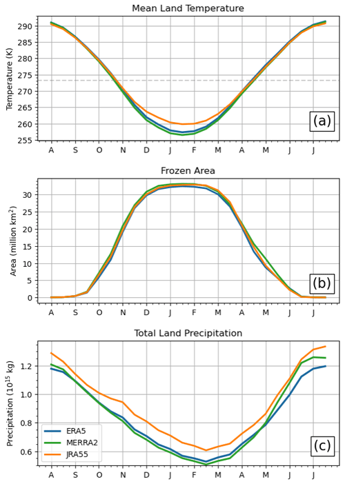
Biases in temperature and precipitation directly impact both online and offline snow products, and our aim is to separately characterize their effects. Briefly comparing temperature and precipitation fields from the three reanalysis products, MERRA-2 exhibits the lowest hemispheric mean land temperatures for most of the year, and JRA-55 exhibits the highest (Fig. 2a). In the winter months, the JRA-55 mean temperature exceeds that of ERA5 by 2.15 K and that of MERRA-2 by nearly 3 K, with the largest temperature difference occurring in January. In addition to being the coldest on average, MERRA-2 has the largest land area capable of sustaining snow, diagnosed as regions with T<0 °C (Fig. 2b). This frozen land area exceeds that of ERA5 by 1 ×10⁶ km² or more during the shoulder seasons of autumn and spring.

With respect to total precipitation, JRA-55 is about 10 % wetter than the other two products across all months (Fig. 2c). MERRA-2 and ERA5 agree more closely, with differences of just 1 % in autumn and spring. ERA5 is 4 % wetter in the winter, and MERRA-2 is about 6 % wetter in the summer months. We investigate the roles of these forcing biases in SWE biases by implementing a simple climatological bias correction (method is described in Sect. S2).

Figure 2 Climatologies of mean temperature, frozen area, and total precipitation over Northern Hemisphere land areas, excluding mountains, computed twice monthly using 14 d windows centred on the 1st and 15th of each month.

2.4 Topography, land mask, and regional definitions

Mountain regions are excluded from our analysis using a mask derived from the Global Earth Topography and Sea Surface Elevation at 30 arcsec resolution digital elevation model (GETASSE30 DEM). Locations in the DEM with local slopes greater than 2° are defined as mountainous. After coarsening the slope mask (to 0.25° × 0.25°, the ERA5 resolution), grid cells that are more than 95 % mountainous are recorded in a binary mountain mask file which is coarsened as needed using a nearest-neighbour algorithm (for the MERRA-2 or JRA-55 grids).

To define land grid cells, we use the land–sea masks associated with each reanalysis. The land fraction is used to scale grid cell land area when computing total snow mass, which depends on SWE and land area. When possible, computations are done on a dataset's native grid, and conservative regridding is applied to the SWE data, conserving total snow mass, before calculating grid-dependent metrics.

2.5 In situ validation of SWE datasets

We evaluate the SWE values from (offline) the B-TIM and (online) reanalysis by comparing them to a combined historical snow course and airborne gamma-derived SWE dataset. These data are independent from snow data assimilated in JRA-55 and ERA5. Snow course observations involve manual measurements of snow depth and density along a predefined transect, with measurements being averaged to obtain a single SWE value for each transect on a specific date (WMO, 2018). The measurement frequency for snow courses varies by jurisdiction, ranging from monthly measurements in Alaska, the western continental US, and most of Finland to measurements every 5 d during the spring snowmelt period in Russia. The Russian network has the highest sampling frequency and is well-distributed across the landscape, while dense networks with lower sampling frequencies are found in Finland, the northeastern US, and parts of southern Canada. Airborne-gamma SWE estimates are calculated by differencing snow-free and snow-covered measurements after accounting for background soil moisture. Flights are 15–20 km long with a 300 m wide footprint. Data are available for the United States and southern parts of some Canadian provinces. There is broad consistency between snow courses and airborne gamma observations (Mortimer et al., 2024), and so we are confident in using both types of information together to evaluate the two types of products.

Using the method in Mortimer et al. (2024), reference SWE data are matched in space and time with the gridded product data. Data are then spatially aggregated and summarized using bias, unbiased root mean squared error (uRMSE), and correlation. We compare data pairs for November through March for all years between 1980 and 2020, aiming to include as many measurements as possible before the snowmelt period. The validation is performed on non-mountainous points with non-zero SWE values below 500 mm that are simultaneously available for the reference data and all the estimates. The latter condition excludes some snow courses in coastal areas due to differing land, ice, and/or water masks and is consistent with our snow mass calculations. In this study, there is no spatial aggregation by land type.

3 Results

We compare snow from global reanalyses (ERA5, ERA5Snow, MERRA-2, and JRA-55) to snow from the offline B-TIM runs. The offline snow products are named BrE5, BrM2, and BrJ55, reflecting the use of distinct reanalysis meteorology for each version but the same B-TIM snow model to produce snow. Two of the reanalysis datasets, ERA5 and ERA5Snow, share the same temperature and precipitation inputs (“meteorology”). Therefore, there is only one BrE5 dataset produced. Standardizing through using a single model means that differences between the offline B-TIM runs primarily reflect differences in the forcing data.

3.1 The B-TIM compares well to in situ observations

Comparing modelled snow to in situ observations is one way to assess the realism and performance of each product. In general, we find a much broader spread in modelled SWE for high reference SWE values, showing overall decreasing model skill with increasing snow depth (Fig. 3a–f). Each scatterplot contains over 200 000 data points. In some products (JRA-55 and MERRA-2), there is a cluster of points where the modelled snow is shallow, but the reference SWE indicates deep snow. The B-TIM products have greater absolute bias than their respective reanalysis products, but they are of comparable magnitude. When mountain points are included, the B-TIM products have lower absolute bias than the reanalyses (not shown). Low bias does not necessarily mean good performance as individual positive and negative differences can cancel each other out. Of the reanalyses, ERA5 and ERA5Snow have the lowest uRMSE and highest correlation compared to the reference values, and so they outperform JRA-55 and MERRA-2 overall. The RMSE (calculated as the bias and uRMSE added in quadrature) of each offline snow product is less than that of its reanalysis counterpart. By these measures, all three B-TIM products have comparable skill to ERA5 and ERA5Snow. Finally, unlike their reanalysis counterparts, BrJ55 and BrM2 do not display the cluster of false low snow values.

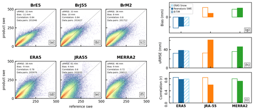
Figure 3 SWE product validation against snow course and gamma SWE measurements. Panels (a)–(f) consist of scatterplots showing all valid data pairs (snow course, product) from November to March over 1980–2018. The scatterplots are coloured as heat maps to display the concentration of data points, which is highest where the colour is red. Summary statistics, including the bias, unbiased root mean squared error (uRMSE), and correlation, are included in the legend and are summarized in (g)–(i).

These validation results show two things. First, the offline products capture realistic snow patterns when compared to ground measurements, even in the context of snow from more complex coupled reanalyses. Second, we see that snow data assimilation does not guarantee skilful snow modelling by these measures. In particular, ERA5 or ERA5Snow and JRA-55 are both produced with snow cover data assimilation (see Sect. 2.2), but while the former two are the best-performing products, the latter performs poorly (with high uRMSE and low correlation) and struggles with both false low snow values and large overestimations relative to ground truth. MERRA-2 does not assimilate snow data but also performs moderately according to the comparison metrics. Additionally, model complexity does not guarantee skilful snow modelling. The offline products generated with the B-TIM, with neither snow data assimilation nor coupled interactions between snow and the land–atmosphere system, perform comparably to each other and to the relatively more complex ERA5 and ERA5Snow, despite differences in the forcing data.

3.2 Using the B-TIM to assess discrepancies between reanalysis snow products

3.2.1 Discrepancies in reanalysis snow climatologies are caused by forcing-data biases

Marked differences appear in the magnitude of total snow mass and snow-covered area for the products considered here. Among the online (the B-TIM) datasets, JRA-55 (BrJ55) has the highest peak snow mass, exceeding the maximum value of MERRA-2 (BrM2) by about 0.15 × 10¹⁵ kg (0.17 × 10¹⁵ kg) and the maximum value of ERA5 (BrE5) by 0.73 × 10¹⁵ kg (0.77 × 10¹⁵ kg), as seen in Fig. 4. The relative rankings of these products and the biases in the peak snow mass are closely reproduced by the offline model; since the offline model can reproduce the biases, we explore the possibility that they are directly caused by the forcing biases discussed in Sect. 2.3, which can equally affect both types of products. We test if these inter-product biases can be manipulated – in particular, minimized – by bias-correcting the meteorological fields used to drive the B-TIM. If biases in mean meteorological conditions are the primary source of snow bias, a correction toward more similar climatological conditions should yield more similar offline modelled snow. We implement a basic multiplicative correction for each month using climatological temperature and precipitation conditions (see the Supplement). Then, for each possible pair (e.g., ERA5 targeting MERRA-2 climatology), three experiments are run: one with adjusted temperature, one with adjusted precipitation, and one with both variables adjusted. This yields 18 datasets in addition to the three unadjusted B-TIM datasets, the three reanalysis datasets, and ERA5Snow.

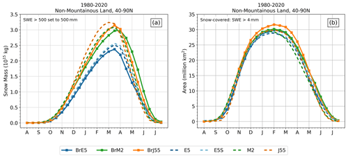
Figure 4 (a) Snow mass climatology over Northern Hemisphere land, with grid cells exceeding 500 mm capped at 500 mm. (b) Snow-covered area climatology, calculated using areas of grid cells with more than 4 mm SWE.

Comparing the bias-adjusted versions of BrE5 and BrM2 (Fig. 5) indicates that temperature biases are the main driver for the differences between ERA5 and MERRA-2 snow mass and snow cover shown in Fig. 4; in the experiments where the ERA5 and MERRA-2 temperature climatologies are bias-adjusted, the resulting snow fields are also much more similar. Precipitation biases play a smaller role, and correcting the precipitation modestly decreases the snow mass biases over the whole season. Snow-covered area is not very sensitive to the precipitation correction, though the best agreement in both cases comes from rescaling both variables. However, mean biases in forcing variables do not explain all the difference in SWE. For the pairs involving JRA-55 (Figs. S1 and S2), the precipitation correction improves the agreement between a dataset and a chosen target but not at the level observed for the ERA5–MERRA-2 pair; the temperature scaling sometimes degrades the agreement. However, JRA-55 is several degrees warmer and about 10 % wetter than the other two reanalyses on average over the region of interest (Fig. 2), constituting more substantial differences than those that exist between ERA5 and MERRA-2.

To summarize, the B-TIM products (BrE5, BrM2, BrJ55) retain the relative biases present in the reanalyses. Motivated by this, we have explored the potential use of bias correction on the meteorological forcing to elucidate the drivers of these snow biases or to correct them to the first order. This approach isolates a subset of drivers and gives insight into the dominant sources of snow biases but requires more refinement to explain biases (see discussion in Sect. 4) more fully.

3.2.2 The B-TIM versions of SWE fields show consistency in seasonal cycle and interannual variability

Aside from JRA-55, which has delayed snow accumulation but an early peak SWE, all the other datasets agree that the snow mass maximum occurs within a 2-week period centred on 15 March. For snow-covered area, all datasets except MERRA-2 peak during the 14 d period centred on 1 February; the MERRA-2 maximum occurs 2 weeks earlier. Thus, unlike the reanalyses, the B-TIM products provide more consistent descriptions of key snowpack climatology metrics.

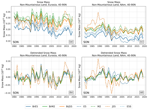
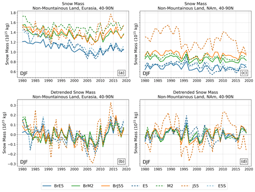
Figure 6 shows the September–October–November (SON) mean snow mass time series, calculated over land regions from 40–90° N (excluding mountains), with the same 500 mm maximum imposed as before to exclude high SWE values over isolated grid cells. Figure 7 shows the December–January–February (DJF) time series of mean snow mass. In these figures, dashed lines are used for reanalysis snow, and the solid lines show offline snow. Even without detrending and removing the mean, it is clear that the solid lines are highly consistent with each other (for both continents and both seasons; panels a and c), while there is much more disagreement between reanalysis products. This highlights the role that factors other than forcing biases play in introducing inter-product differences. We quantify the consistency in the offline–offline and reanalysis–reanalysis pairs by calculating correlation coefficients after removing the least-squares linear fit (Fig. 8). Detrending by other methods yields similar results (e.g., using the Theil–Sen estimator, which is robust with respect to outliers and shifts to the start and end of the time series, not shown). Across all regions and all seasons, the B-TIM products are strongly correlated with one another (r>0.85), whereas the reanalysis r values are lower in general and greatly depend on the pair.

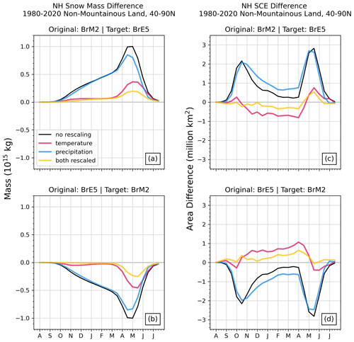
Figure 5 (a, b) NH snow mass and (c, d) snow cover extent differences for MERRA-2 and ERA5 calculated as original minus target. Each panel shows the difference between the original and target snow mass climatologies (black), and the coloured lines represent the datasets generated by adjusting temperature (pink), precipitation (blue), or both (yellow) to the target dataset's climatology.

Figure 6 Time series of total snow mass for SON by continent. Lower row has linear trends removed.

The reanalysis JRA-55 snow mass is unique, characterized by large decadal variations. Positive anomalies are most common from 1980 to 1994 and from 2010 to 2020, while negative anomalies occur from 1995 to 2009 (Fig. 7d). These inconsistencies are not as extreme over Eurasia as JRA-55 captures positive and negative anomalies that are mostly in agreement with the remaining datasets, but its variations have the greatest magnitude (e.g., 1991, 2014). The disagreement is substantial in terms of snow mass amount. Over North America, especially before 1995, the reanalysis JRA-55 dataset has as much as 50 % more snow mass than the other reanalyses. This behaviour is not present in BrJ55. Additional comparison with in situ data indicates that the version of JRA-55 that has less interannual variability (BrJ55, solid orange) also has a significantly lower RMSE and higher correlation with the in situ data than the native JRA-55 (dashed orange; Fig. S3).

We now return to consider the two versions of the ERA5 reanalysis: ERA5 and ERA5Snow (dashed, blue in two shades, Figs. 6 and 7). The two time series diverge due to a change in the snow cover extent data assimilation in 2004. The mean difference in DJF snow mass over North America between these two products is 5 times greater after 2004 compared to before 2004 (9×10¹³ and 1.8×10¹³ kg, respectively) and 3 times greater after 2004 for Eurasia (7.7×10¹³ kg compared with 2.4×10¹³ kg). This step change is problematic for trend and correlation assessments, and so we use ERA5Snow in Fig. 9 below. As an offline product, BrE5 does not display the step change in 2004.

Figure 7 Time series of total snow mass for DJF by continent. Lower row has linear trends removed.

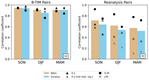
Figure 8 (a) Correlation coefficients for the B-TIM dataset pairs. Individual values are shown with black points, and the mean is represented by the height of the bar to summarize the group. Similar information is shown in (b) for the reanalysis dataset pairs.

These two examples show that the B-TIM snow datasets can generate reasonably performing benchmark datasets which are useful to contrast against native snow data. The comparison between reanalysis and the offline product forced with the same meteorology can highlight spurious variability, as in the case of JRA-55, or can point to temporal inhomogeneities, as with ERA5.

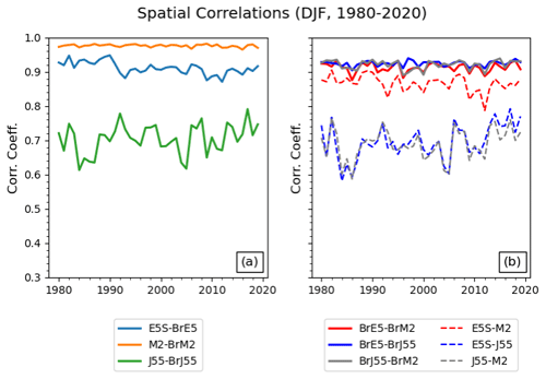
The consistency found for the offline products extends to spatial patterns. The time series of the DJF spatial pattern correlation between dataset pairs is shown in Fig. 9, with SON values shown in Fig. S4. For both seasons, offline–offline pairs are the most consistent with each other (with the highest r values) despite different meteorological forcings. There is also evidence of spatial disagreement between some of the reanalysis products. Notably, JRA-55 is very different from all the other datasets. This can be seen with the ERA5Snow–JRA-55 and MERRA-2–JRA-55 pairs (different model, different forcing), which have the weakest spatial correlations, or with the BrJ55–JRA-55 pair (different model, same forcing), which has a much lower correlation compared to the other same-forcing pairs. We remind the reader that ERA5Snow is used instead of ERA5 as the reanalysis snow product with the aim of removing the discontinuity around 2004; the meteorology is the same in both products so ERA5Snow can be compared to BrE5. The pattern correlations appear to be stable across the 40-year period for all pairs, although those involving JRA-55 have larger year-to-year variability. Additionally, reanalysis and offline versions of JRA-55 snow have low spatial correlation across all seasons and both continents compared to the ERA5 and MERRA-2 (Fig. S5). Broadly, reanalysis and offline patterns are less similar over Eurasia for a given season, and the correlation decreases over the snow year.

Figure 9 Spatial correlations for DJF calculated between pairs of datasets with the same meteorology (a) and between pairs of similar type (b) (either offline–offline or reanalysis–reanalysis).

4 Discussion and conclusions

We can summarize our key points as follows:

• An updated and more complete description of the B-TIM offline snow model has been provided for the first time since 2003, accompanied by an open-source code release of the model implemented in Python.

• The offline B-TIM snow generated using meteorological forcing from three reanalysis products has been validated against an independent set of in situ snow observations (Sect. 2.5). The offline products perform generally as well as (online coupled) reanalysis snow. Based on this result, datasets generated with the B-TIM are treated as reasonably performing benchmark estimates of historical snow and are used to investigate discrepancies in reanalysis SWE.

• Compared to online reanalysis snow, the offline B-TIM snow yields far more consistent interannual variability for both aggregate and spatially resolved snow metrics. This suggests the potential utility of the B-TIM as an offline tool for simplified snow modelling in seasonal to decadal prediction systems and climate downscaling for impact analysis.

• Climatological characteristics of the offline B-TIM snow are generally more consistent with one another for various measures than reanalysis snow despite differences in the meteorological forcing data. Using the B-TIM with bias-adjusted forcing, climatological SWE differences between ERA5 and MERRA-2 are found to primarily come from temperature biases (MERRA-2 is colder, resulting in more SWE throughout the snow season). Attribution of discrepancies in terms of JRA-55 with the other two reanalyses is not as straightforward, as we discuss next.

Offline modelling has allowed us to understand some of the components contributing to the spread in SWE estimates across these three reanalyses. In general, nonlinearities inherent to snow modelling mean that it is unclear how exactly meteorological biases will impact modelled SWE fields for both historical and modelled future snow conditions (Evan and Eisenman, 2021; Räisänen, 2023; Sospedra-Alfonso and Merryfield, 2017). Interpreting the causes of SWE differences is further complicated when comparing products produced using different snow models and different data assimilation schemes. In this sense, the B-TIM can easily generate simplified benchmark datasets (no data assimilation and a single, simple model) alongside more complex products of interest. Here, we have attempted to attribute climatological SWE biases to climatological meteorological biases by adjusting each of the two forcing variables and calculating the effect on the SWE. We have taken advantage of the B-TIM's speed, which has allowed us to perform many cross-tests.

Future work should continue developing the B-TIM through systematic testing of parameter values. For example, the spatial variability and sensitivity of the model to the 20 % precipitation loss have not recently been characterized. This type of work is possible due to the recent increases in the availability and quality of in situ SWE, snow depth, and snow density information (Vionnet et al., 2021) for validation. Forcing biases and parameter changes both strongly influence modelled snow (Cho et al., 2022; Essery, 2015; Günther et al., 2019; Menard et al., 2021), and they should be characterized for the B-TIM. However, offline modelling can broadly be seen as a tool to investigate snow biases in products where additional simulations are not feasible, as is the case for reanalysis.

The simple bias adjustment methodology we use requires more refinement to fully explain the biases. Large differences between a dataset and a chosen target may make the multiplicative scaling less suitable, for example, by changing the input variable distributions significantly. Additionally, other aspects that are not captured in mean conditions can influence SWE in models, such as the nature of the diurnal cycle in temperature and the distribution of precipitation intensity and/or duration (or a combination of the two). Multiplicative rescaling can affect these aspects when adjusting a dataset to a chosen target, with the greatest impact coming from adjusting both driving variables at once. These effects are most relevant at the shoulder seasons and for areas with ephemeral snow.

Using reference in situ data and inter-dataset consistency arguments, we have shown that terrestrial SWE taken directly from the JRA-55 reanalysis is problematic and should not be used for climate analysis. Unlike the BrJ55 product, which performs comparably to the BrE5 and BrM2 products, the reanalysis JRA-55 terrestrial snow product is the least accurate with respect to the in situ validation. Furthermore, the interannual variability of the JRA-55 snow mass anomaly time series (Figs. 5 and 6) and corresponding SWE field patterns (Fig. 7) differ greatly from all the other datasets. The strong performance of BrJ55 suggests that the problem with JRA-55 snow arises from the JRA-55 snow model and data assimilation.

Snow is a critical component of the climate system, influencing a range of environmental and societal processes. Accurate snow modelling is needed for applications that require a long time series (e.g., trend analysis) and the best instantaneous estimates of SWE (e.g., numerical weather prediction). Here, we have demonstrated the value of a simple model like the B-TIM in helping us assess new products against self-consistent benchmarks as they are released. These considerations will continue to be important as we look ahead to the next generation of global reanalyses, including the JMA Reanalysis for Three Quarters of a Century, which is now available (JRA-3Q; Kosaka et al., 2024), and ERA6 (Balsamo et al., 2023).