the Creative Commons Attribution 4.0 License.
the Creative Commons Attribution 4.0 License.
 | 09 Oct 2024
The grain-scale signature of isotopic diffusion in ice
Diffusion limits the survival of climate signals on the water stable isotopes in ice sheets. Diffusive smoothing acts not only on annual signals near the surface, but also on long-timescale signals at depth as they shorten to decimetres or centimetres. Short-circuiting of the slow diffusion in crystal grains by fast diffusion along liquid veins can explain the “excess diffusion” found on some ice-core isotopic records. But experimental evidence is lacking as to whether this mechanism operates as theorised; theories of the short-circuiting also under-explore the role of diffusion along grain boundaries. The non-uniform patterns of isotopic deviation δ across crystal grains induced by short-circuiting offer a testable prediction of these theories. Here, we extend the modelling for grain boundaries (and veins) and calculate these patterns for different grain-boundary diffusivities and thicknesses, temperatures, and vein-water flow velocities. Two isotopic patterns are shown to prevail in ice of millimetre grain size: (i) an axisymmetric “pole” pattern with excursions in δ centred on triple junctions, in the case of thin, low-diffusivity grain boundaries, and (ii) a “spoke” pattern with excursions around triple junctions showing the impression of grain boundaries, when these are thick and highly diffusive. The excursions have widths ∼ 10 %–50 % of the grain radius and variations in δ ∼ 10−2 to 10−1 times the bulk isotopic signal for oxygen and deuterium, which set the minimum measurement capability needed to detect the patterns. We examine how the predicted patterns vary with depth through a signal wavelength to suggest an experimental procedure, based on laser ablation mapping, of testing ice-core samples for these signatures of isotopic short-circuiting. Because our model accounts for veins and grain boundaries, its predicted enhancement factor (quantifying the level of excess diffusion) characterises the bulk-ice isotopic diffusivity more comprehensively than past studies.
- Article
(11028 KB) - Full-text XML
-
Supplement
(2046 KB) - BibTeX
- EndNote


The water stable isotope records (δ18O, δD) in polar ice cores contain diverse palaeoclimatic signals. Owing to isotopic diffusion in firn and ice, signals at decimetre and centimetre or shorter scales experience pronounced smoothing as they descend the ice column. This post-depositional process limits the integrity and resolution of climatic information at different depths. The smoothing rate needs to be known for recovering the original (e.g. annual) δ variations at the surface by “back-diffusing” an isotopic record (Johnsen, 1977), for reconstructing surface temperatures in the past from spectrally derived diffusion lengths (Gkinis et al., 2014), and for predicting how deep climatic signals of different timescales survive in an ice core (e.g. Grisart et al., 2022). The last aspect, which matters particularly for long records, is of major interest to the ongoing ice-coring campaigns at Little Dome C, East Antarctica, which aim to retrieve ice reaching back ≈ 1–1.5 Ma; see the Beyond EPICA – Oldest Ice project web page (BE-OI, 2017) and the Million Year Ice Core project web page (MYIC, 2020).
“Excess diffusion” in the ice below the firn is a key concern in this subject. Analysis of the Greenland Ice Core Project (GRIP) ice core by Johnsen et al. (1997, 2000) showed that the annual δ18O signals in the Holocene section of this core decay ≈ 10–30 times faster than expected from the self-diffusion rate measured in single ice crystals (Ramseier, 1967), implying a large enhancement of the bulk-ice isotopic diffusivity above the monocrystalline diffusivity. Theories put forward to explain this excess diffusion invoke short-circuiting – the idea that, in polycrystalline ice, fast diffusion in the network of liquid veins (located at triple junctions) and along grain boundaries bypasses the slow diffusion within ice grains to cause the enhancement. After Nye (1998) made pioneering calculations to show that the presence of veins causes excess diffusion by short-circuiting, Johnsen et al. (2000) adapted the firn isotope diffusion model of Whillans and Grootes (1985) to gauge the separate contributions of grain boundaries and veins to the mechanism. Later, Rempel and Wettlaufer (2003) refined Nye's model to account for the finite isotopic diffusivity of the vein water; they calculated the diffusivity enhancement in ice at °C as a function of signal wavelength, grain size, and vein radius. In a recent study, Ng (2023) extended the Nye–Rempel–Wettlaufer framework to show that water flow in the veins amplifies excess diffusion and that vein-water flow velocities of ∼ 101–102 m yr−1 yield a 10- to 100-fold enhancement, able to explain the GRIP findings and sections of ice with anomalously high diffusion lengths found in the EPICA (European Project for Ice Coring in Antarctica) Dome C ice core by Pol et al. (2010) and found in the WAIS (West Antarctic Ice Sheet) Divide ice core by Jones et al. (2017) – which these authors interpreted as signs of excess diffusion potentially caused by the short-circuiting mechanism. As pointed out by Ng (2023), the modulation of isotopic diffusion by vein-water flow means that the decay of climate signals at each ice-core site depends on the hydrology and connectivity of veins down the ice column, as well as the ice temperature, grain and vein sizes, and recrystallisation processes affecting these geometries.
Here, we take the modelling of excess diffusion in a new direction to enable a critical research gap to be addressed. Besides those records displaying signs of excess diffusion (accelerated signal decay or anomalous diffusion lengths) and motivating the theories in the first place, no direct observations have been made to show that isotopic short-circuiting actually operates. Independent evidence is needed to verify the mechanism at the grain scale, for ice-core samples deemed affected by excess diffusion, and for polycrystalline ice generally. One way of testing the theories is to compare their predicted signal smoothing rate against the rate measured in ice doped with isotopic signals, but the slowness of diffusion makes such experiments prohibitively long at low temperature. A different laboratory-based approach, proposed herein, is to analyse ice affected by excess diffusion to look for the distinct grain-scale isotopic variations which the theories predict to result from short-circuiting. For instance, the theories of Nye (1998), Rempel and Wettlaufer (2003), and Ng (2023) – capturing the isotopic exchange between veins and ice in the absence of grain boundaries – imply axisymmetric patterns of δ around veins, which may be used for this purpose. Knowledge of these patterns is a prerequisite to testing for short-circuiting this way. It also helps researchers developing techniques of making high-resolution isotopic measurements on ice, who currently lack information on how strong or weak the grain-scale variations in δ might be. Predicting the variety of isotopic patterns thus forms the main goal of this paper, although we leave the laboratory testing to future studies.
To simulate realistic patterns, we go beyond Nye (1998), Johnsen et al. (2000), Rempel and Wettlaufer (2003), and Ng (2023) by formulating a continuum model that includes grain boundaries, coupling diffusion across all three components: ice, veins, and grain boundaries. This integrated model is necessary, as we wish to test the four theories collectively, and each of them is missing some elements (e.g. Johnsen et al. (2000) did not couple together veins and grain boundaries, whereas the other theories neglected grain boundaries). However, we mean to examine the short-circuiting conceived in these theories, so we do not build more sophistication into the model to account for every conceivable process in polycrystalline ice. We are not trying to advance a new theory to describe isotopic diffusion in the most complete manner possible.
The model geometry, which remains simplified, allows us to explore the combined effect of veins and grain boundaries on the bulk-ice isotopic diffusivity. An outstanding question in this regard is whether diffusion along grain boundaries matters in ice with glaciological grain sizes (∼ mm). Their effect on the bulk diffusivity is assumed to be significant in ultrafine-grained ice with ≈ 10–30 nm sized crystals (Lu et al., 2009), where grain-boundary surfaces have a high volumetric density (Jones et al., 2017). In contrast, for glacier ice, a much weaker effect may be suspected based on the calculations of Johnsen et al. (2000), who estimated that the grain boundaries in the GRIP Holocene ice (mean grain diameter ≈ 3 mm) need to be unrealistically thick (50 nm) to explain the observed excess diffusion, even if they are liquid films with the high isotopic diffusivity of water. Studying this question with a fully coupled model has not been done before and forms our second goal. We compute the enhancement factor f for ice of millimetre grain size at −32 and −52 °C (which approximate the upper-column temperatures at the GRIP and EPICA core sites, respectively) for different grain-boundary properties and vein-water flow velocities.
Including grain boundaries in the modelling brings challenges. Most obviously, the grain-boundary thickness c and grain-boundary diffusivity Db need to be specified, but, as we will elaborate in Sect. 2, these parameters are not well constrained. In our calculations, we cover potential scenarios by experimenting with different assumptions for c and Db in a sensitivity analysis. Another issue is that the model geometry does not permit an analytical solution, unlike in the theories of Nye (1998), Rempel and Wettlaufer (2003), and Ng (2023). We tackle this by developing a bespoke numerical solution method.
The paper is organised as follows. Section 2 details our model formulation and solution method. Section 3 presents the computed isotopic patterns and enhancement factors for a range of parameters, including the end-member cases of thick, diffusive and thin, non-diffusive grain boundaries and intermediate scenarios. In Sect. 4, we discuss the prospects of detecting the isotopic signatures of excess diffusion in laboratory measurements on ice, focussing on techniques based on laser ablation (LA) sampling (e.g. Malegiannaki et al., 2023). Readers keen to see the predicted patterns are advised to turn to Figs. 4–11. Those seeking to compute the diffusivity enhancement factor for conditions not covered by us can find our numerical code in the repository linked to the paper.
The importance of testing the theories cannot be understated, and several points are worth emphasising on this note before we start. Given the idea of querying the short-circuiting mechanism, we do not claim that the modelled patterns will necessarily be found – or found at the predicted amplitudes – during grain-scale testing of ice. And, while the mechanism has not been experimentally confirmed, ice-core studies seeking to understand excess diffusion on specific isotopic records should not automatically invoke it as if it were firmly established. With those core sections showing excess diffusion at GRIP, EPICA Dome C, and the WAIS Divide, their explanation by means of vein or grain-boundary short-circuiting remains plausible, but tentative, and the causal factors (e.g. why excess diffusion apparently occurs in those sections and not others) are unclear. In terms of probing the origin of excess diffusion at those sites, the most advanced analyses to date are probably the ones by Jones et al. (2017) and Ng (2023), who used models of the enhancement factor to calculate diffusion lengths to inform hypotheses about the cause. We refer the reader to these studies for more details on this subject.
2.1 Model geometry
We use the setup in Fig. 1a – adapted from Nye (1998), Rempel and Wettlaufer (2003) and Ng (2023) – which represents ice-crystal grains surrounding a vein by a vertical annular cylinder, in , where r is the radial coordinate, a is the vein radius (∼ µm), and b approximates the mean grain radius (∼ mm). The water vein is kept liquid by dissolved ionic impurities, which lower the melting point (Mulvaney et al., 1988; Nye, 1991; Mader, 1992b). We consider depth-varying isotopic signals in the bulk ice, with z denoting depth. For a list of mathematical symbols used in this paper, see Table A1 in the Appendix.
Grain boundaries leading from the vein are modelled as planes of thickness c(≪a) at θ= 0, L, and 2L, where θ is the azimuth and . Introducing them makes the problem non-axisymmetric, but their periodicity means that it suffices to solve the model in .
In plan view, the cylinder approximates a unit cell centred upon triple junctions in ice whose structure is idealised as honeycomb-like (Fig. 1b). In this picture, the radius b reaches out roughly half-way along each grain boundary or to the middle of grains; for convenience, we refer to r≈b at either location as the “interior”. As in the theories of Nye (1998), Rempel and Wettlaufer (2003), and Ng (2023), our extended model geometry still idealises many aspects of the real system: (1) it ignores the detailed vein cross-section, which consists of three convex walls (Nye, 1989; Mader, 1992a; Ng, 2021), although their small length scale implies perturbations only to the local isotopic concentrations near r=a; (2) veins and grain boundaries are assumed stationary rather than migrating under recrystallisation processes; and (3) horizontal or near-horizontal veins and grain boundaries are disregarded, so the model does not account for additional short-circuiting arising from these boundaries, which may distort the isotopic patterns near them and affect the enhancement factor. We discuss the last two limitations in Sect. 4.
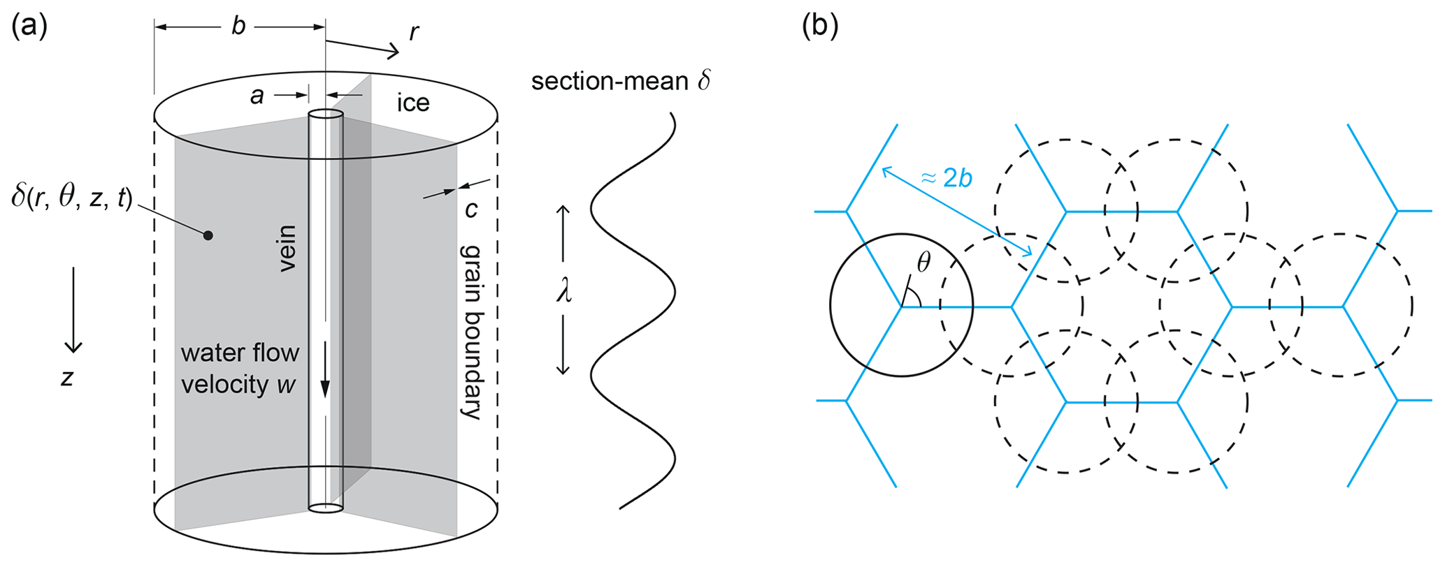
Figure 1(a) Model geometry for calculating coupled isotopic diffusion in ice, vein, and grain boundaries near a triple junction. (b) Approximate view of what the cell in panel (a) represents in polycrystalline ice with hexagonal grains.
2.2 Material properties
Prior to modelling signal evolution, we consider the isotopic diffusivities in the three components (ice, vein water, grain boundaries) and the grain-boundary thickness and, where relevant, explain values chosen for simulations. All diffusivities discussed here – referring to molecular diffusion – are applicable to the transport of oxygen and deuterium.
For the isotopic diffusivity in ice or “solid diffusivity” Ds, we use Ramseier's (1967) formula for self-diffusion in single ice crystals:
in which T denotes temperature in kelvins. For the isotopic diffusivity in vein water or “liquid diffusivity” Dv, we use the composite exponential formula:
This formula was derived by Ng (2023) by fitting self-diffusivity data between −12.8 and −60.8 °C, which Xu et al. (2016) obtained by modelling crystal growth rates measured in laboratory experiments. Equation (2) is consistent with the established formula of Gillen et al. (1972) for T down to −31 °C but covers a greater temperature range. Figure 2 plots Eqs. (1) and (2). These formulas neither account for pressure dependence, which should cause only a minor correction under the glaciostatic overburden in ice sheets (a few percent on Dv; Prielmeier et al., 1988), nor for the influence of dissolved impurities, whose characterisation is presently very limited. Thus, Ds and Dv might vary from the formulas. However, the temperature dependencies shown in Fig. 2 should be robust, and departures from the formulas by a few times (e.g. see uncertainty for Ds indicated by Lu et al. (2009) in their Fig. 8) or even 1 order of magnitude are much smaller than the diffusivity contrast ∼ 106, which governs the qualitative interactions during vein short-circuiting.

Figure 2Arrhenius plot of the isotopic diffusivities Ds (ice), Dv (vein water), and Db (grain boundaries). The curves for Ds and Dv come from Eqs. (1) and (2). The dashed blue curve plots the relation of Gillen et al. (1972) for Dv. The blue cross locates the diffusivity used by Johnsen et al. (2000) (Sect. 2.2). The box and whiskers at −2 °C (bar: likely range; whiskers: maximal range) and the inclined black line (dashed box: uncertainty range) plot the laboratory-based estimates for Db of Lu et al. (2007, 2009). The star plots Db at 250 K from molecular dynamical simulation (Yagasaki et al., 2020). To pose values of Db for modelling at −32 and −52 °C, we extrapolate the trend of the results in Lu et al. (2009) to those temperatures and expand the uncertainty to form two sets of grain-boundary diffusivities (circles; values in Table 2), which we address by using descriptive labels (grey wording). Grey lines indicate the same system of referring to the size of Db at other temperatures.
What of the grain-boundary diffusivity Db and thickness c? The physicochemical influences on these parameters are poorly understood across the range of ice-core temperatures (≈ 0 to −55 °C); their values are uncertain and lack reliable formulas. Several empirical and theoretical constraints come to our rescue, as detailed below. But first we sketch more background on the grain-boundary properties of ice as a step towards explaining our choices for these parameters.
Grain boundaries are disordered interfaces between crystals. Determining their properties experimentally is difficult because the microscopic scale concerned often means that a property can only be inferred from bulk measurements that mix crystal and grain-boundary effects (e.g. Lu et al., 2007). In ice, the grain-boundary thickness must be at least several times the crystal lattice spacing (O–O distance: 0.276 nm; Hobbs, 1974). It may be higher in the presence of impurities (Thomson et al., 2013) but is generally expected to depend in complex ways on impurity type and concentration (Benatov and Wettlaufer, 2004). Premelting occurs at high temperatures (Dash et al., 2006): that is, grain boundaries thicken and start to exhibit quasi-liquid behaviour near the melting point Tm as this is approached from below, at to ∼ 10 K. Grain-boundary premelting in ice has been studied by (i) theoretical modelling of the forces and thermodynamics controlling the premelted film thickness (Wettlaufer, 1999; Benatov and Wettlaufer, 2004), (ii) laboratory measurements of the film thickness (Thomson et al., 2013), and (iii) classical molecular dynamical simulations (e.g. Moreira et al., 2018). Premelting in ice diminishes beyond a few degrees below Tm and is expected to be negligible below °C. For instance, Lu et al. (2007, 2009) argued from experimental results for Db (reported below) that premelting does not occur below −2 °C in pure ice, although it starts to occur at 8 °C in ice doped with HCl at 0.04 % by mass (≈ 0.01 M bulk concentration). On the other hand, the notion of premelted grain boundaries features in the theories of excess diffusion by Johnsen et al. (2000) and Rempel and Wettlaufer (2003), even though their analyses considered much colder ice. Johnsen et al. (2000) in particular referred to the grain boundaries in ice at °C as “supercooled water films” and took the liquid diffusivity Dv at that temperature ( m2 s−1; blue cross in Fig. 2) to be the grain-boundary diffusivity Db in calculations. As we will see, this estimate for Db is probably too high.
The question whether grain boundaries in ice are watery or more like solid lattice has a bearing on where isotope fractionation (during phase change) is envisaged to occur in the system – whether at (1) the transition between them and the crystal lattice within the grain interior or (2) where they meet veins. If one assumes grain boundaries to be liquid, then fractionation occurs at the liquid–solid phase change at location 1, not at location 2, where there is no phase change. If one envisages them to be solid, closely resembling crystal lattice, then fractionation occurs at location 2 and not (or negligibly) at location 1. In our model, we assume the latter scenario because our simulations explore temperatures far below the premelting regime, making the former scenario less plausible (the fractionation coefficients will be described in Sect. 2.3). Note, however, that the question is unsettled given the lack of experimental determination, and fractionation may occur at both places in reality (e.g. in a hybrid scenario where grain boundaries have microstructural properties in an intermediate state between solid and liquid).
We turn to the parameter choices, treating grain-boundary thickness c first. Information comes from two sources. Thomson et al. (2013) used optical scattering to measure c in ice at °C with different dissolved impurity concentrations (NaCl) and different grain-boundary orientations. The impurity concentration at grain boundaries was estimated from the bulk concentration, as it cannot be measured directly. They found c from 1 to 8 nm, generally increasing with impurity level (this factor promotes interfacial molecular disorder) for different crystal misorientation angles. For °C, no experimental measurements of c have been made so far, but molecular-scale dynamical simulations offer a handle. Yagasaki et al. (2020) used the TIP4P/Ice model to study molecular transport at grain boundaries in impurity-free ice at 250 K ( °C) and found c∼1 nm under a variety of conditions. Given these studies, we choose three values of c for our modelling: 1, 5, and 10 nm (Table 1). The highest value accounts for the possibility of thick grain boundaries resulting from high impurity levels.
For the grain-boundary diffusivity Db, we rely on guidance from the experimental results of Lu et al. (2007, 2009), which are the only results available to date on ice. For T from −18 to −1 °C, these authors determined that Db lies intermediate between Ds and Dv, several orders of magnitude from each of them (Fig. 2). Their experiments measured the inter-diffusivity Deff of H and D in nanocrystalline sandwiches of ice by monitoring the reaction zones at the interfaces with thermal desorption spectroscopy, a technique that ablates the ice with laser and analyses the vapour composition. They estimated Db from Deff by a model inversion based on the Hart–Mortlock equation (Deff as a linear combination of the component diffusivities, weighted by the component volume fractions). In their 2007 study, conducted at −2 °C, their Db estimate spans 3 orders of magnitude, although they suggested a likely range of 1–2 orders (bar and whiskers in Fig. 2). Their 2009 study extended the measurements of Db down to −18 °C (sloping black line in Fig. 2), with an uncertainty of 1 order of magnitude on either side, finding for Db an Arrhenius-type temperature dependence with an activation energy of ≈ 69 kJ mol−1.
Table 1Grain-boundary thicknesses investigated in our modelling.

Table 2Isotopic diffusivities (in m2 s−1) used in our modelling. At each temperature, we study five values of the grain-boundary diffusivity, Db.

Below −18 °C, Db has not been experimentally measured. To pose Db at −32 and −52 °C for modelling, we extrapolate the estimates of Lu et al. (2009) down the Arrhenius trend (Fig. 2), assuming the same activation energy and Db to lie between Ds and Dv at lower temperatures. This approach finds support in the modelled value of Db at 250 K from Yagasaki et al. (2020) (star in Fig. 2). However, we widen the uncertainty range of the Lu et al. (2009) estimates by 1 order of magnitude because (i) the Hart–Mortlock equation crudely approximates the bulk diffusivity,1 and the version of the equation used in their inversion ignores the presence of veins, and (ii) they showed that doping the ice with HCl increased Deff by ≈ 20 times above the pure-ice value, indicating that dissolved impurities can raise Db substantially. Uncertainties in their inversion from assumptions about the grain-boundary width are also discussed by Lu et al. (2007). Based on the extrapolation, we choose two sets of five values for Db (circles in Fig. 2): one set for −32 °C and the other set for −52 °C, as listed in Table 2. In each set, which span a generous range for sensitivity analysis, the middle three values of Db represent direct extrapolations of the laboratory measurements and the uncertainty range of Lu et al. (2009). The lowest and highest values, respectively, mimic the more extreme scenarios of coupled diffusion near the no-grain-boundary limit and of high impurity concentration at grain boundaries. For convenience, we refer to the values in each set as low, medium-low, medium, medium-high, and high (Fig. 2, Table 2). This descriptive scale for Db is applicable to other temperatures (grey lines in Fig. 2) on the basis of the assumed trend. We explore select values of Db and c in this paper, given the impracticality of covering a large number of parameter combinations when computing isotopic patterns and enhancement factors.
That Db is bracketed by Ds and Dv corroborates insights from classical molecular dynamical simulations. Moreira et al. (2018) found that, a few degrees below Tm, the simulated molecular transport along premelted grain boundaries resembles diffusion in glassy systems and is sub-diffusive in character (with mean-square displacement of molecules ∼ tγ, where t denotes time and γ<1), reflecting lateral confinement of the grain boundaries by the adjacent crystal lattice. The grain boundaries at 250 K simulated by Yagasaki et al. (2020) structurally resemble low-density liquid water. Besides estimating a corresponding value for Db, Yagasaki et al. (2020) studied diffusion along triple junctions, finding a diffusivity of 3.4 Db for them. We cannot adopt this as the vein diffusivity Dv because their model does not recognise water-filled veins at triple junctions, whose presence in ice has been confirmed by optical (Mader, 1992a) and nuclear magnetic resonance (Brox et al., 2015) methods.
2.3 Continuum formulation
For the system in Fig. 1, let us denote the concentrations of a trace isotope (18O or D) in the ice, vein, and grain boundaries by , Nv(z,t), and , respectively, where t is time. We assume Nv to be independent of r and θ and assume Nb to be uniform across the grain-boundary thickness. The concentrations satisfy the conservation equations
where w is the vein-water flow velocity in the downward (z-) direction; other symbols have been introduced. These equations account for isotopic exchange across the vein wall, between grain boundaries and vein, and between grain boundaries and ice. Respectively, the second-last term in Eq. (4), the last term in Eq. (5), and the last term in Eq. (4) – which are source terms in those equations – describe the isotope fluxes leaving the ice radially and azimuthally and leaving the grain boundaries radially. The factor 3 sums flux contributions to the vein from all directions. Taylor dispersion along the vein is ignored, as the corresponding Péclet number (≲ 10−1) would only raise the vein liquid diffusivity by < 0.1 %. We specify the boundary conditions at r=b (zero gradient in the interior) and anticipate at r=a (because the vein wall at different azimuths contacts the same vein isotopic concentration). Rotational periodicity implies solution symmetry in about .
Deriving a model for the isotopic deviation δ follows the method of Rempel and Wettlaufer (2003). If Ns0, Nv0, and Nb0 are the number densities of the major isotope (16O or H) in the three components, then fractionation at the vein wall and at the vein end of grain boundaries yields , where α is the fractionation coefficient. Following Rempel and Wettlaufer (2003), we assume equilibrium fractionation. Following them also, we will set α=1, which seems to be a plausible approximation because α(18O 16O) ≈ 1.0029 and α (D H) ≈ 1.021 at 0 °C (O'Neil, 1968; Árnason, 1969; Lehmann and Siegenthaler, 1991), but note that the temperature dependence of α in T<0 °C for either element is unknown.2 We assume no fractionation on the side walls of grain boundaries (Sect. 2.2), so in r≥a. By rewriting Eqs. (4) and (5) in terms of Ns (with taken as constant), eliminating their time derivatives with Eq. (3), and using the definition
we obtain the diffusion equation
with the boundary conditions
The boundary conditions in Eqs. (9) and (10), derived from Eqs. (4) and (5), encapsulate advection and diffusion along the vein and diffusion within the grain-boundary planes. The boundary condition at θ=L is met automatically, given the solution symmetry. We have introduced the thinness parameter
which measures the grain-boundary thickness scaled to the vein radius. The parameters
quantify the diffusivity contrasts of water to ice and grain boundary to ice, respectively. As noted in Sect. 2.2, typically βv∼106 (Fig. 2); βb (< βv) is also large, but it depends on the chosen grain-boundary diffusivity. Note that one cannot lump all grain-boundary properties into a single parameter (e.g. the diffusivity–thickness product cDb or ε(βb+1)) in this model.
The partial differential equation problem for δ in Eqs. (7) to (10) is linear. To quantify signal decay, we study how sinusoidal signals of different wavelength λ (or wavenumber ) smooth out in time (Nye, 1998; Rempel and Wettlaufer, 2003; Ng, 2023) by posing the trial solution
where is a complex decay-rate parameter. The enhancement factor measuring the level of excess diffusion is given by the ratio of the signal decay rate DsζR in Eq. (13) to the baseline decay rate in monocrystalline ice (ice without grain boundaries and veins). On defining , the enhancement factor is
In Eq. (13), the function determines the spatial pattern of isotopic signals in three dimensions (3D). At depth z, Re[Hexp (ikzz)] gives their amplitude across the annular sector , , and the section-mean isotopic signal (ignoring the exponential time decay factor) is
The sinusoidal signals at different radii and azimuths have the phase angle . Therefore, when ζI is non-zero, the signals migrate at the velocity in the z direction.
2.4 Scaled model
When addressing isotopic patterns later, it will be useful to reference the features on them (e.g. size or radial position) to the grain radius b. To facilitate this, we non-dimensionalise the model by letting
at the same time scaling other variables as follows:
The scaled-model equivalent to Eqs. (7) to (10) is then
where we have dropped the stars for convenience (we work with dimensionless variables from now on). The parameter
is the dimensionless vein radius ( in glacier ice translates to ), and
is a Péclet number measuring the importance of vein-flow-driven advection relative to solid-state diffusion. The trial solution in Eq. (13) becomes
while Eq. (14) for the enhancement factor f is unchanged under the scaling.
2.5 Eigenvalue problem
The pattern H(r,θ) for signals of any wavenumber kz remains to be solved. Substituting δ from Eq. (21) into Eq. (18) leads to
with the boundary conditions
We have defined
and introduced the parameters
Equations (24) and (25) may be further simplified by using Eq. (22) to reduce the number of high-order derivatives; thus, we find
and
Equations (22), (23), (28), and (29) need to be solved to determine the isotopic patterns. They constitute a homogeneous boundary value problem for H with the eigenvalue s2, whose real part leads to the enhancement factor (see Eqs. 26 and 14) and whose imaginary part ζI is non-zero if the vein water flows (w, χ≠0); thus, vein-water flow causes the signals to migrate in the same direction, as in the model of Ng (2023). The slowest-decaying eigenmode (with minimum Re(s2)>0) yields the desired pattern, as the other eigenmodes decay faster, leaving this mode to be observed in long time. The problem is non-trivial because of mixed boundary conditions at the vein wall and grain boundaries. A solution by the separation of variables H=H1(r)H2(θ) could exploit the periodicity in θ for H2; equivalently, one could take the cosine transform azimuthally (e.g. and the Hankel transform in the radial direction. However, we find that an analytic solution does not seem feasible by these conventional approaches – a fundamental obstacle being mismatch between the Fourier kernel of the grain-boundary condition in Eq. (29) and the Hankel kernel of the differential operator in Eq. (22). We therefore solve the problem numerically. Readers not interested in the associated details might skip to the last paragraph of Sect. 2.6.
2.6 Numerical method
We use the pseudo-spectral method, employing Chebyshev collocation in the θ direction to achieve “spectral accuracy” in approximating the solution (Boyd, 2000; Trefethen, 2000). Although the angular periodicity suggests using trigonometric basis functions instead (i.e. Fourier spectral method), the corresponding approximation lacks spectral accuracy and converges much more slowly than Chebyshev polynomials, as H is non-smooth (with discontinuous gradient) across the grain boundaries. We use the finite-difference approximation in the radial direction.
The solution on each grain boundary can be written as . This enables us to work with alternative variables by splitting H into the sum
where the field F represents variations in the ice sector unaccounted for by G. Usefully, F is zero along the grain boundaries and on the vein wall (as there). The decomposition converts Eqs. (22) and (23) to the partial differential equation
with the homogeneous boundary conditions
Meanwhile, Eqs. (29) and (28) become the ordinary differential equation
with boundary conditions at the vein wall and in the grain interior given by
We have used the prime (subscript) notation to denote ordinary (partial) derivatives above. The differential equations for G and F are coupled via their source terms.
Because the vein short-circuits diffusion in the ice, we expect the solution to vary rapidly just outside the vein wall and slowly in the grain interior, notably away from grain boundaries. To resolve the variations near r=ξ (vein wall) with sufficient grid points, without over-introducing grid points in the interior (which slows numerical computation), we make a change to the radial variable
The interior and the vein wall are located at R=1 and , respectively (Fig. 3a).

Figure 3Elements of the mixed spectral–finite difference numerical method. (a) Radial coordinate transformation used to increase spatial resolution near the vein. (b) Numerical grid for F(R,x). Filled dots indicate solution points; open circles indicate zero boundary values. (c) The same grid points on the ice domain. Panels (b) and (c) are illustrative; we use many more grid points (N=100, J=201) than shown.
Next, we set up the Chebyshev collocation points
choosing
such that the interval maps onto the angular range of the sector (Fig. 3b, c). With these transformations, the coupled problem for F and G becomes
and
We have written these results with s2 on the right-hand side to facilitate the eigenvalue calculation.
The method proceeds by discretising the x axis with the Chebyshev points and the R axis as J equidistant points (Fig. 3b) and by using the spectral differentiation matrix of Trefethen (2000; p. 53) and finite differencing to compute derivatives in these respective directions. With F zero on three edges of the solution domain, there are unknowns in Fn,j and J unknowns in Gj for and . The scheme converts Eqs. (39) and (40) into a system of linear equations Mv=s2v, where the solution eigenvector (a column vector)
has elements, and M is a sparse-banded matrix (detailed in Sect. S1 and Fig. S1 in the Supplement). After using the MATLAB function eig to compute s2 from M, we find v corresponding to the slowest-decaying eigenmode and put Fn,j and Gj back in cylindrical polar coordinates to build the solution H. Our computation used N=100 and J=201 points, and we checked for numerical convergence and convergence at diminishing grain-boundary thickness c towards the analytic solution of Ng (2023), which describes the vein-only system without grain boundaries.
All isotopic patterns reported below display H after it has been regridded at a constant θ spacing by Lagrange interpolation from the Chebyshev grid values, normalised by the value of H at r=1, , and copied from into the other sectors to fill the ice annulus. At r=1, , a position which we call the “mid-grain interior”, the vertical sinusoidal signal in δ has maximum amplitude because diffusion short-circuiting subdues the signal amplitude more strongly elsewhere, especially near the vein and grain boundaries. Consequently, the mid-grain interior signal closely approximates and has a slightly higher amplitude than the bulk vertical isotopic signal in Eq. (15) derived through horizontal averaging or, equivalently, the signal measured by ice-core continuous flow analysis (CFA) (Kaufmann et al., 2008; Bigler et al., 2011). The normalisation thus puts our pattern amplitudes in Sect. 3.1 in a dimensionless unit, scaled (approximately) to the bulk vertical signal. It allows the absolute amplitude of the δ variations in the predicted patterns to be inferred for any bulk-signal amplitude.
We proceed to examine computed isotopic patterns (Sect. 3.1) and bulk-diffusivity enhancement factors (Sect. 3.2) for different model parameters. In our model runs, we set the vein and grain sizes at a=1 µm and b=1 mm and assume the fractionation coefficient α=1 so that the results can be compared with those of Rempel and Wettlaufer (2003) and Ng (2023) and applied to either δ18O or δD. Using precise fractionation coefficients at 0 °C (≈ 1.0029 for oxygen, ≈ 1.021 for hydrogen; Sect. 2.3) changes the results numerically in a minor way that does not alter our qualitative findings. We will report only briefly on the qualitative effects of changing a and b, which were examined in more detail by Rempel and Wettlaufer (2003).
There are 30 parameter combinations from the choices of temperatures T (−32 °C, −52 °C), grain-boundary thicknesses c (1, 5, 10 nm; Table 1), and grain-boundary diffusivities Db (Table 2). For each combination, we compute results for signal wavelengths λ across the range 0.005–0.15 m and different vein-water flow velocities w in 0–50 m yr−1 when °C and 0–5 m yr−1 when °C. These ranges enable study of the enhancement factor f as a function of λ and w in Sect. 3.2. Note that w at ice-core sites is unknown and has not been measured (Ng, 2023). We chose the w ranges here based on flow velocities of ∼ 101 m yr−1 in micrometres-thick veins that Nye and Frank (1973) estimated in their theory of water percolation in ice sheets and the expectation that blockage or disconnection of the vein network (e.g. by dust particles) can drastically reduce w.
In Sect. 3.1, we analyse selected runs to highlight the effect of grain-scale short-circuiting on the isotopic patterns, focussing on results for λ=10 cm. This wavelength is chosen for illustration because (i) short signals at λ∼10–30 cm are common in the isotopic records from polar ice cores, (ii) the shortest surviving signals (despite stronger diffusive smoothing at smaller λ) are of interest, and (iii) some signals with λ as short as 10 cm are found in the high-resolution (5 mm) records from the WAIS Divide (δ18O and δD; Jones et al., 2017) and the South Pole (δ17O, δ18O, and δD; Steig et al., 2021). Perusing other ice-core datasets, we do not find signals at λ≤10 cm in the NGRIP δ18O record (Gkinis et al., 2014; 5 cm resolution), whereas the GRIP δ18O record (Johnsen et al., 1997; 55 cm resolution) and EPICA Dome C δD record (Grisart et al., 2022; 11 cm resolution) are too coarse for discerning signals at λ≈10 cm. However, the Dye-3 ice core exhibits annual variations in δ18O and δD as short as a few centimetres (Vinther et al., 2006; down to ≈ 2 cm in their Fig. 6 and ≈ 5 cm in their Fig. 5).
When addressing grain-boundary properties below, we use the qualitative descriptors for Db and c introduced earlier (Fig. 2; Tables 1 and 2). Not all parameter combinations will be analysed for their isotopic patterns, e.g. not the patterns for medium-low Db, which typically resemble and fall between the low and medium Db cases. As we shall see, the more interesting pattern transitions occur as Db varies from medium to high.
3.1 Isotopic patterns in 3D
3.1.1 Archetypal patterns at −32 °C: effects of grain-boundary properties and vein-water flow
Figure 4 shows the predicted patterns at °C, λ=10 cm, and w=0 for three runs with intermediate (5 nm thick) grain boundaries having high, medium-high, and medium diffusivities. They illustrate the change from an axisymmetric “pole” pattern to a “three-spoke” pattern as Db increases, which is one of our key findings. We use the word “spoke” as an analogy to the radial elements of a bicycle wheel; “pole” refers to a central peak without such elements. In each panel, the colour charts show the dimensionless variations in δ – i.e. Re[H(r,θ)exp (ikzz)] after normalisation by (Sect. 2.6) – at three depths in the range spanning 1λ. We look down the domain in Fig. 1a and take horizontal slices of its isotopic deviation, analogous to cuts perpendicular to a vertical triple junction in ice. The far-left plot shows depth profiles of isotopic variations at the mid-grain interior (r=1, ; black curve), at the grain-boundary interior (r=1, θ=0; blue), and along the vein (red). The first profile always has unit amplitude under the normalisation; in these runs, the latter two profiles have amplitudes very slightly less than 1, so they obscure the first profile when plotted. To emphasise where fast changes occur on each pattern, the colour scale is always fitted to its maximal range of variations, and we use one of two colour schemes depending on whether δ at the vein is higher or lower than δ in the interior. Note that the isotopic signals decay in time following Eqs. (13) and (21) and that the patterns occur on a background (mean) isotopic concentration that would first be subtracted when studying real ice samples.

Figure 4Horizontal isotopic patterns computed in three model runs with °C, λ=10 cm, c=5 nm, w=0 m yr−1, and Db= (a) 1.5 × 10⁻¹¹ m2 s−1, (b) 1.5 × 10⁻¹² m2 s−1, and (c) 1.5 × 10⁻¹³ m2 s−1, compiled by sampling the δ variations in the annular domain of Fig. 1a at three depths (z1, z2, z3). The colour charts reach out to the ice grain radius; the vein at the centre is too small to be visible. One of two colour schemes is used, depending on whether δ at the vein exceeds δ in the grain interior or vice versa. In each run, the δ variations are normalised by the value of δ in the mid-grain interior at z=0 (Sect. 2.6), so the colour-scale numbering and amplitudes are dimensionless. On the far left, curves show the depth profiles of δ variations at three sites – the vein wall (red), grain-boundary interior (blue), and mid-grain interior (black) – over a signal wavelength. The curves have very similar amplitudes in these runs, so the red curve overlies the other two. White and grey bars indicate the distinct depth intervals where the vein-versus-interior difference in δ has the same sign. The enhancement factors in these runs are f= (a) 3.37, (b) 2.70, and (c) 2.64.
First, we analyse Fig. 4b (the medium-high diffusivity run) to explain salient features and how the patterns relate to the short-circuiting. This solution shows overall what the axisymmetric theories (Nye, 1998; Rempel and Wettlaufer, 2003; Ng, 2023) predict, with isotopes diffusing radially towards the vein (e.g. at z=z1, z3), up and down along the vein, and back into ice and radially outwards (z2). As in those theories, these exchanges bypass solid diffusion in the ice to cause excess diffusion and accelerate the signal decay – the computed enhancement factor f is 2.70 (> 1) – and they induce radial variations in δ that are the most rapid immediately outside the vein. These δ excursions cause the pole (z2) and reverse-pole (z1, z3) patterns, which respectively reflect the role of the vein as a source and sink of isotopes in different horizontal sections in the short-circuiting.
The distinct depth intervals where isotopes diffuse radially inwards and outwards (identified by where δ in the ice exceeds δ in the vein and vice versa) are indicated by white and grey bars on the far-left plot. In each interval, the patterns' strength (magnitude of horizontal isotopic variations) varies with depth according to the difference in δ between the vein and interior, but the patterns themselves hardly change with depth, except very near the transitions where the difference in δ between vein and interior changes sign (i.e. transitions between the bars). This near invariance arises because λ≫b so that, away from these transitions, vertical gradients in δ are much smaller than horizontal gradients in the system, and the diffusion problems determining the pattern at different depths are similar.3 At the transitions, as the vein-to-interior difference in δ switches sign, the pattern flips from a pole to a reverse pole or the other way. Movie S1 shows the complete pattern evolution over 1λ. The stable “archetypal patterns” in the white and grey depth intervals are paired, with the same form but opposite polarity, so hereafter we write “pole” for both pole and reverse pole. Detailed examination shows that, within a narrow distance about each transition, the pattern evolves continuously, with a pole weakening to zero strength and reversing sign. This behaviour is not resolved in Movie S1 but can be gauged from its dynamic colour ranges.
The poles in Fig. 4b are not axisymmetric: they exhibit deformities reflecting the grain boundaries, whose impression is faint in this case. In contrast, Fig. 4a (high-diffusivity run, where Db is 10-fold) shows a much stronger grain-boundary imprint that causes three-spoke patterns. Here, the vein plays a similar short-circuiting role as before: the archetypal patterns again flip where the vein-to-interior difference in δ switches sign. But isotopes also diffuse from ice to grain boundaries and along them to the vein (vice versa at other depths), and diffusion occurs vertically within the grain boundaries. Fast diffusion along them extends the poles to form the spokes and cause extra short-circuiting across the ice sectors, which raises the excess diffusion (f=3.37). The 3D isotopic field is more complex than in the run of Fig. 4b. Azimuthal variations are evident from the spokes, which indicate difference in δ between the ice interior and the grain-boundary interior. The strongest azimuthal gradients occur just outside the vein next to grain boundaries, so lateral short-circuiting dominates near each ice sector's apex. The increased short-circuiting also reduces the vein-to-interior difference in δ compared to the last run (see colour-scale numbering).
Going the other way, lowering Db to medium diffusivity (Fig. 4c) suppresses the grain-boundary imprint and shrinks the poles, which still show corners but only at tiny radii. These changes are expected given the diminishing diffusion along grain boundaries. Although this solution thus closely approximates the axisymmetric solution of Rempel and Wettlaufer (2003) and Ng (2023), its f value (2.64) is slightly less than what they found (2.65) for the same conditions in the absence of grain boundaries; this is also the case if Db is further reduced to medium-low or low. In other words, as we increase Db from the solid diffusivity Ds, f decreases before rising. The initial decrease is due to radial short-circuiting of the ice near crystal apices by the grain boundaries, which reduces the radial gradients in isotopic concentration there and thus the vein's short-circuiting effect; we will see more drastic examples of this behaviour shortly (Fig. 6). For the interested reader, Movies S2 and S3 document the depth-evolving isotopic patterns in the runs of Fig. 4a and c.

Figure 5Archetypal isotopic patterns computed in two model runs assuming °C, λ=10 cm, c=10 nm, w=0 m yr−1, and Db= (a) 1.5 × 10⁻¹¹ m2 s−1 and (b) 1.5 × 10⁻¹² m2 s−1, sampled at the same depths as those in Fig. 4 (z1, z2, and z3) and shown with the scheme used there. The enhancement factors in these runs are f= (a) 4.06 and (b) 2.77.

Figure 6Archetypal isotopic patterns computed in four runs with °C, λ=10 cm and w=5 m yr−1 (downward vein-water flow) and the grain-boundary properties (a) m2 s−1, c=5 nm; (b) Db=1.5 × 10⁻¹² m2 s−1, c=5 nm; (c) Db=1.5 × 10⁻¹¹ m2 s−1, c=10 nm; and (d) Db=1.5 × 10⁻¹² m2 s−1, c=10 nm. The layout of Fig. 4 is used, but only the depths z2 and z3 are sampled, and we omit the colour range on each pattern, which is defined by the difference between the vertical isotopic profiles (curves on the far left) for the vein wall (red), grain-boundary interior (blue), and mid-grain interior (black); the black curves are overlain by the blue curves in these runs. As in Fig. 4, all signal amplitudes are dimensionless. The enhancement factors in these runs are f= (a) 4.56, (b) 5.96, (c) 4.97, and (d) 5.33.
Next, we vary the grain-boundary thickness c. Figure 5 presents archetypal patterns in two runs at −32 °C assuming thick grain boundaries (c=10 nm) of high and medium-high diffusivities. Compared to the runs in Fig. 4a and b, which use the same Db values, these patterns have more developed grain-boundary imprints and enlarged central excursions, and the associated enhancement factors are higher. As expected, thickening the grain boundaries here has a similar effect to raising Db in terms of enhancing grain-boundary short-circuiting, so the transition from a pole to a three-spoke pattern occurs at lower diffusivity. We experimented also with thin grain boundaries (c=1 nm), finding in this case that the pole-to-spoke transition shifts to higher diffusivity instead. The corresponding archetypal patterns will feature in Fig. 9, described later.
All experiments so far assume no vein-water flow, so their vertical isotopic variations at different positions (r, θ) are in phase (curves in Fig. 4). What if w≠0? Figure 6 shows the results of four runs assuming intermediate and thick grain boundaries with high and medium-high diffusivities, where we set w to 5 m yr−1, leaving other parameters unchanged. Ng (2023) explained that vein-water flow displaces the vein signal against the interior signal to induce a “shear layer” of phase-shifted isotopic variations outside the vein wall. In turn, the shear layer generates strong radial gradients in isotopic concentration in the ice near the vein, amplifying the diffusive isotope exchange between ice and vein to raise the level of excess diffusion. Figure 6 shows the vein signal displaced in all four runs. Each solution still has two transitions where the vein-to-interior difference in δ switches sign and has paired archetypal patterns occupying equal depth intervals, within 1λ. The archetypal patterns closely resemble the ones found earlier (cf. Figs. 4a–b and 5) because the vein-flow-induced shear layers cause only subtle changes to them. Figure 7 depicts the shear layer on a map of ϕ for the run in Fig. 6a, showing also the radial transects of H at θ=0 and . The non-zero imaginary part of H causes a phase shift reaching by the vein in this run. Unlike in the axisymmetric theory of Ng (2023), the shear layer here is triangular (non-circular) in planform due to lateral short-circuiting by the grain boundaries, so isotopic transport in 3D is complicated by both vein-water flow and the grain boundaries' presence.

Figure 7(a) Map of signal phase angle ϕ at z=0 in the experiment of Fig. 6a. Corresponding radial transects of (b, c) the real and imaginary parts of the normalised solution H and of (d) ϕ at z=0, on θ=0 (black; i.e. grain boundary) and (red). The location lines in panel (a) and the curves in the other panels use the same colour-coding.
All four experiments in Fig. 6 confirm the amplification of excess diffusion by w anticipated by Ng's study: at each combination of c and Db, f is higher than in the runs where w=0 (cf. Figs. 4a–b and 5). Three effects involving the shear layer are noteworthy. First, Fig. 6 shows that, at fixed c, f is actually reduced as Db increases from medium-high to high. This arises from grain-boundary short-circuiting of the ice-crystal apices, which, in these runs, limits the radial isotopic gradients of the shear layers so much that the reduced exchange between vein and ice offsets the enhanced exchange between grain boundaries and ice. Specifically, the higher Db is, the weaker those gradients are at w=5 m yr−1, so the lower f is. This behaviour, which is observed in other runs with vein-water flow (e.g. f values in red in Figs. 9 and 10), will be revisited in Sect. 3.2.
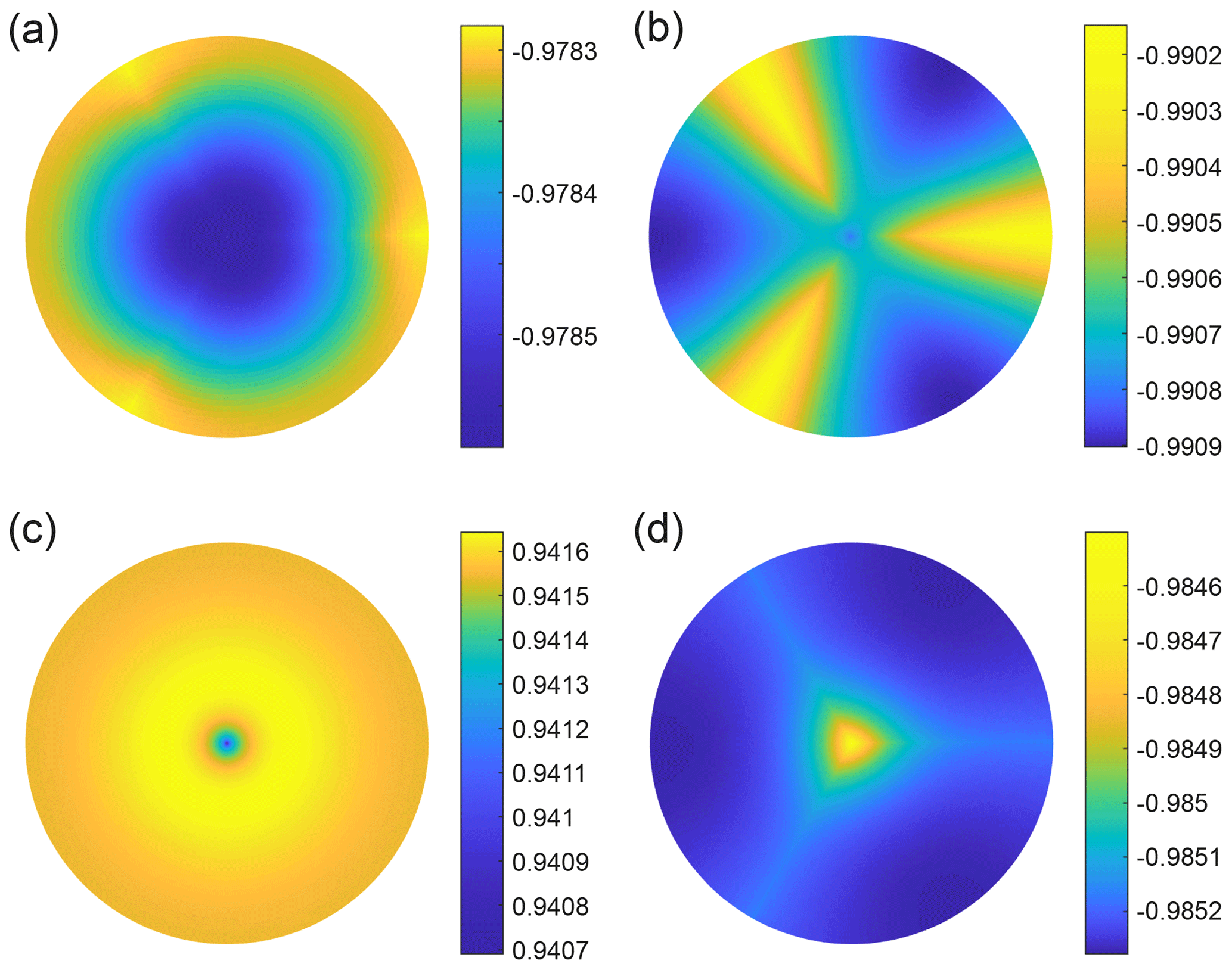
Figure 8Transitory isotopic patterns from (a, b, d) three of the runs in Fig. 6 (see reference labels there) and (c) a run with °C, λ=10 cm, w=5 m yr−1, c=1 nm, and m2 s−1. The patterns have low amplitudes because they occur near transitions in z across which the vein-to-interior difference in δ switches sign. As before, the colour scales are dimensionless.
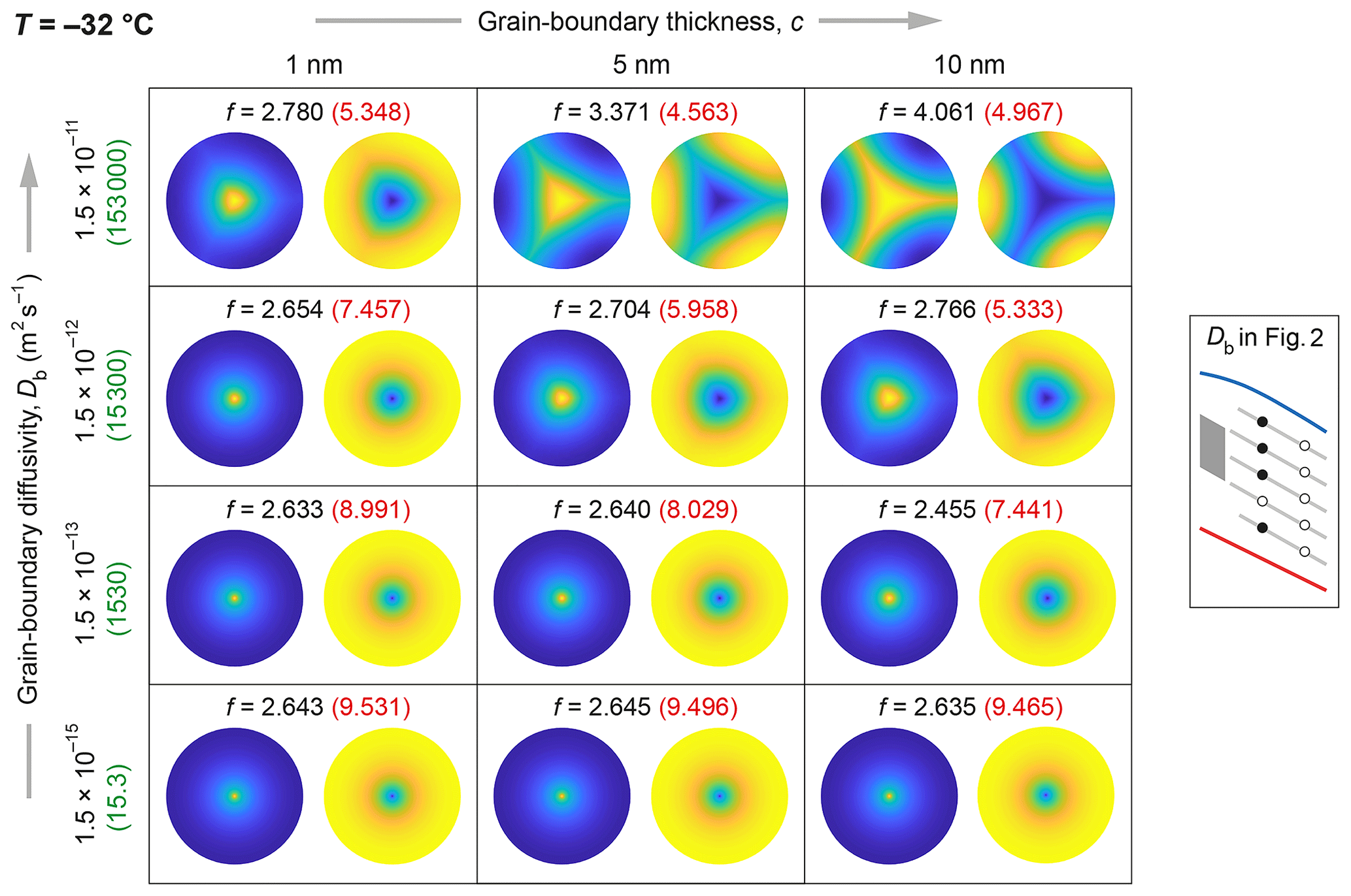
Figure 9Dependence of archetypal patterns on grain-boundary diffusivity Db and thickness c at −32 °C for signals with the wavelength λ= 10 cm. The key on the right locates the four values of Db as filled black circles on the scheme of Fig. 2. Numbers in green give the corresponding diffusivity contrasts βb. The isotopic patterns and the enhancement factors f in black are for w=0. Bracketed in red are the f values when vein water flows at w=5 m yr−1, which produces patterns only slightly different from the ones shown (Figs. 6 and S4).

Figure 10Dependence of archetypal patterns on Db and c at °C and λ=10 cm. The layout of Fig. 9 is used here. The isotopic patterns and the enhancement factors f in black are for w=0. Bracketed in red are the f values for vein-water flow at w=0.5 m yr−1, which produces patterns only slightly different from the ones shown (Fig. S5).
Second, the vertical phase shifts between the vein and interior signals increase the amplitude difference between these signals at most depths, thereby strengthening the isotopic patterns (e.g. compare the curves in Fig. 6b to those in Fig. 4b). Vein-water flow thus makes the patterns easier to detect, even though it affects their form only in minor ways. Additional runs at w>5 m yr−1 (not reported) show further increase in the phase shifts and pattern amplitudes with w. Note that higher pattern amplitudes also result from shorter signal wavelength (e.g. Figs. S2 and S3 in Sect. S2, which show repeats of the runs in Figs. 4 and 6 for λ=2 cm) or larger grain size (e.g. Figs. S6 and S7 in Sect. S4, which show repeats of the same runs for b=5 mm), but how λ and b affect the anatomy of the 3D isotopic fields will not be analysed extensively herein.
Third, when w≠0, the phase variations cause unusual patterns to appear in the narrow transitions across which an archetypal pattern (pole or spoke) evolves into its opposite form. Figure 8 shows examples of these patterns, taken from the last runs and an extra run at medium Db. They include “wheels” with notable azimuthal variations mid-way along grain boundaries (near θ=0, L, and 2L at r≈1) and “halos” where isotopic concentration varies with radius non-monotonically. Although we mention them for completeness, we expect to find them rarely in measurements because their small amplitudes likely fall below measurement sensitivity and the sampling has to be made at precisely the right depth against the bulk signal.
3.1.2 Pattern continuum at different temperatures
Returning to the archetypal patterns, we summarise and elaborate on the insights gained so far on them with the aid of Fig. 9, which puts them in the c–Db parameter space. The pattern type at −32 °C depends on the relative amount of vein and grain-boundary short-circuiting. Thin, non-diffusive grain boundaries give a pole pattern, since the short-circuiting is done mostly by the vein. The axisymmetric solution is reproduced at the no-grain-boundary limit c→0 (dimensionlessly, ε→0) or when Db→Ds (grain boundaries with the solid diffusivity; βb→0). Thick, diffusive grain boundaries give three-spoke patterns, as they serve as radial extensions of the vein in the 3D isotopic exchange; the higher c or Db is, the more developed the spokes are. On the pattern continuum, the pole-to-spoke transition at −32 °C occurs roughly at medium-high Db – higher if the grain boundary is thinner. Figure 9 also indicates that a 10-fold increase in c or Db leads to almost the same pattern, suggesting the thickness–diffusivity product entirely determines the pattern. However, our model analysis (Sect. 2.3) shows that cDb (or ε(βb+1)) is not the sole control; c and Db also act independently, which is why the 10-fold increases do not give identical enhancement factors.
How about other temperatures? Calculations at −52 °C for 10 cm long signals reveal a similar array of archetypal pole and spoke patterns in the parameter space (Fig. 10; cf. Fig. 9). Vein-water flow again modifies these patterns slightly (Fig. S5) but increases their amplitude and detectability strongly (we find this at other temperatures). That the pattern arrays for −52 and −32 °C bear a close resemblance is unsurprising because the diffusivity contrast predominantly determines the pattern at each thickness c and because our Db values for the two temperatures lie at similar distances above the solid-diffusivity curve (Fig. 2) and convert to similar βb values (Figs. 9 and 10). The liquid diffusivity Dv also influences the patterns, but βv varies weakly with T, as Dv(T) and Ds(T) have similar slopes on the Arrhenius plot (Fig. 2). These considerations mean that we can predict the isotopic pattern at any temperature from Db and c by calculating βb – or gauging it with Fig. 2 – and consulting the arrays in Figs. 9 and 10. For example, at –42 °C, for grain boundaries with Db= 10−14 m2 s−1, Eqs. (1) and (12) give βb≈ 400, while these T–Db data plot between the grey lines labelled medium-low and medium in Fig. 2. Both evaluations put the grain-boundary diffusivity between medium-low and medium on our descriptive scale, below the third row of patterns in Figs. 9 and 10, so we predict a pole pattern (regardless of the grain-boundary thickness). An interesting corollary is that isotopic patterns observed in real ice can be used to infer grain-boundary properties (Sect. 4.1).
Hitherto, we have focussed on using the results at λ=10 cm to elucidate underlying interactions and pattern controls. For signals of other wavelengths at centimetre and decimetre scale, we find similar effects of Db and c on the archetypal patterns; e.g. see Figs. S2 and S3 for results at λ=2 cm. The patterns are weakly sensitive to λ for the reason given earlier (footnote 3). When λ≫b, as is typical of isotopic signals in ice sheets, the diffusion problem for δ at different depths (within a signal wavelength) is similar, dominated by horizontal gradients, with terms representing vertical gradients being negligible. Note that our results in this section show that a given isotopic pattern does not indicate a fixed enhancement factor, as it can form under different conditions (T, λ, and Db and c combinations).
3.1.3 On pattern detectability
We end the section with a few remarks related to pattern detection, in preparation for the work in Sect. 4.1. Since the patterns in Figs. 4 to 10 are based on the normalised H, their δ variation in absolute terms is given by their dimensionless amplitude, as shown by the colour scales or the difference between the vein and grain-interior isotopic profiles, multiplied by the true amplitude of the bulk vertical signal. This scaling conversion applies to both oxygen and deuterium. For instance, if the bulk signal (in δ18O or δD) is 10 ‰ peak to peak, then the pattern amplitudes in Fig. 4b, ≈ 0.005–0.007, translate to δ variations ≈ 0.025 ‰–0.035 ‰, whereas the much higher pattern amplitudes in the runs with vein-water flow in Fig. 6b and d, ≈ 0.1, translate to ≈ 0.5‰. Each result here is an approximation and underestimation because the bulk signal has a scaled amplitude ≲ 1 (see the end of Sect. 2.6); we do not quantify the approximation exactly as it varies with the pattern. The δ excursions of the patterns reported above have widths ∼ 10 %–50 % of the grain radius b. Although we do not study grain-size effects extensively, additional runs show that this qualitative finding holds at b=5 mm (Figs. S6–S9); thus, the δ excursions are dimensionally wider in coarse-grained ice. However, the pattern forms shift nearer the pole end of the pole-to-spoke continuum as b increases (Figs. S6–S9). This is predicted by the scaled model (Sect. 2.4), where a larger b has no effect on βb (this is the dominant control on pattern type; Sect. 3.1.2), reduces the dimensionless signal wavelength (the pattern is only weakly sensitive to this), raises the Péclet number χ (the flow-induced shear layer does not strongly alter the pattern; Sect. 3.1.1), and reduces the thinness ξ and εξ of the vein and grain boundaries and thus their short-circuiting efficiency; this causes the shift.
Finally, surface and thin sections on real ice will often cross triple junctions at oblique angles to their axes, yielding distorted isotopic patterns for them. Figure 11 exemplifies potential outcomes, made by sampling the solutions in Figs. 4a and 6a–b at tilts of 5, 10, 25, and 50° from the horizontal (Movies S4–S7 show how they evolve as the azimuth of the section normal varies). While this examination stretches our use of an idealised model geometry, which ignores the irregular shape of real grain boundaries and triple junctions (e.g. neighbouring junctions in real ice typically differ in orientation), these examples suggest that poles and spokes may still have visible impressions at moderate tilt. Generally, though, on a given section, only some triple junctions have low or moderate tilts; other junctions with high tilts will have unrecognisable isotopic patterns.

Figure 11Isotopic patterns compiled by sampling several solutions in Figs. 4 and 6 at non-zero tilt from the horizontal (constant z in our model), with the sampled sections meeting z=z2 at r=0. The tilt angle, tilt-axis azimuth, and model run are indicated in each case. As before, the colour scales are dimensionless.
3.2 Enhancement factor in bulk-ice diffusivity
Also of interest is how much the presence of grain boundaries affects the enhancement factor f measuring the excess diffusion (and acceleration of signal smoothing) above the rate due to monocrystalline diffusion. Here, we study this by examining the computed surfaces of f as functions of vein-water flow velocity w and signal wavelength λ.
Ng (2023) reported the surfaces f(w, λ) at and −52 °C for the axisymmetric (vein-only) system when a=1 µm and b=1 mm, which we reproduce in Fig. 12a and e as contour maps. Our computed surfaces accounting for grain boundaries show the same valley form as these maps, with f increasing with λ and . Thus, vein-water flow amplifies excess diffusion in our system with grain boundaries by an amount independent of whether the flow is up or down, as in the vein-only system. Our model also predicts known trends of f against the vein and grain sizes – f increases with a and decreases with b (Rempel and Wettlaufer, 2003), which reflects the way these parameters control the efficiency and density of short-circuiting elements (Ng, 2023). Notably, a larger b increases these elements' spacing relative to the signal wavelength and so reduces the short-circuiting and f towards 1 (no excess diffusion) asymptotically; this dependence is shown in Fig. 4 of Rempel and Wettlaufer (2003) for the vein-only system. Although we do not characterise this dependence in our system fully, model runs at b from 1 to 5 mm in 1 mm increments confirm a similar behaviour (Fig. S10, Sect. S4). Furthermore, our system exhibits (i) lower f at −52 °C than −32 °C when w=0 and (ii) stronger modulation of f by w in colder ice (this is why our experiments at −52 °C use lower vein-flow velocities; e.g. compare the f values in Fig. 10 resulting from w=0.5 m yr−1 to those in Fig. 9 from w=5 m yr−1). These aspects have been explained by Ng (2023) with scaling arguments that we do not repeat here.
We focus instead on how the surface f(w, λ) deforms when we introduce grain boundaries and vary their diffusivity. Figure 12b–d and f–h present the results at −32 and −52 °C for intermediate grain boundaries with medium, medium-high, and high Db. The results are shown as difference maps Δf(w, λ) referenced to the surfaces in Fig. 12a and e because we find visualising the changes by comparing different sets of contours of f more difficult.4 On the difference maps, the interesting feature is the wedges of negative Δf straddling the w=0 axis. They indicate reductions in f caused by grain-boundary diffusion when vein water flows. The reductions increase in magnitude with Db and λ, occur at relatively low vein-water velocities in λ≳2.5 cm, and persist to higher vein-water velocities the longer the signal is. Between each pair of wedges is a narrow ridge at w≈ 0 where Δf≳0, which matches our finding in Sect. 3.1 that f typically increases with the degree of grain-boundary short-circuiting at zero vein flow (e.g. f values in black in Figs. 9 and 10). Outside the wedges, Δf is positive and increases steeply with .

Figure 12Impact of the presence and diffusivity (Db) of grain boundaries on the level of excess diffusion for different vein-flow velocities w and signal wavelengths λ at −32 and −52 °C when c=5 nm. (a, e) Contour maps of enhancement factor f(w, λ) for the vein-only system without grain boundaries; data from Ng (2023). (b–d) f(w, λ) reported as contour maps of the difference Δf from panel (a) for our system at −32 °C when the grain boundaries have medium, medium-high, and high diffusivities. (f–h) Ditto for −52 °C but referenced to panel (e).
For the surfaces f(w, λ), these differences mean that grain-boundary short-circuiting flattens their valley bottom – reducing f there compared to the vein-only case for signals longer than ≈ 2.5 cm, while it raises f only at sufficiently high vein-flow velocities. Because our runs at λ=10 cm with vein-water flow (Sect. 3.1) assume values of w inside the wedges, they predict less excess diffusion and lower f when Db is increased (f values in red in Figs. 9 and 10). The mechanism was explained in Sect. 3.1 through study of the 3D isotopic fields: with vein-water flow, diffusion along grain boundaries suppresses the flow-induced shear layer by radial short-circuiting of its concentration gradients. The outcome thus rests on a competition: at low , this effect overcomes the enhanced isotopic exchange between ice and vein due to the shear layer (so f decreases overall); it is out-competed by the latter at high (whereupon f increases). The wedge shape arises because the mechanism is more effective for longer signals, which develop weaker shear layers at a given w. For completeness, we provide the computed grids of f in the paper's repository and show in Fig. S11 a companion version of Fig. 12 that plots f instead of Δf.
In summary, although short-circuiting by diffusive grain boundaries leaves a stable three spokes on isotopic patterns (Sect. 3.1), for decimetre-scale isotopic signals, it increases f only at zero or high vein-water velocities, not at intermediate velocities. Thus, while the presence of grain boundaries or veins in glacier ice (b∼ mm) always causes excess diffusion compared to the monocrystal, and while vein-water flow always increases the level of excess diffusion compared to no flow, whether more diffusive grain boundaries amplify the level has a mixed answer. However, this outcome does not affect the concept of using the grain-scale patterns to diagnose isotopic short-circuiting.
4.1 Detecting isotopic patterns
Our calculations establish isotopic patterns around triple junctions as an inevitable consequence of excess diffusion that operates by vein and/or grain boundary short-circuiting. As highlighted in the Introduction, we propose looking for this grain-scale prediction in laboratory measurements on ice to test the Nye–Rempel–Wettlaufer genre of theories. Here we discuss this matter, drawing on the results in Sect. 3.1.
The crux is whether such tests reveal systematic excursions in δ around veins and grain boundaries like the predicted archetypal patterns. Also relevant is whether pole or three-spoke patterns (or both) are found to prevail in natural ice, but the current level of knowledge about the grain-boundary properties of ice precludes a clear expectation on this. Our model predicts a pattern type dependent on grain-boundary diffusivity and thickness – higher Db and c favour spokes. In particular, medium-high to high Db in our descriptive range (Fig. 2) is needed for spokes (Figs. 9 and 10; also, Figs. S2–S3 and S6–S9). This does not necessarily mean that spokes will rarely be observed, given substantial uncertainties about the extent to which impurities and crystallographic factors affect Db and c (Sect. 2.2). Also, although the HCl bulk concentration (≈ 0.01 M) used by Lu et al. (2009) in their diffusivity measurements to explore the impurity effect is much higher than the typical concentration of Cl− in ice cores (∼ 1–10 µM), natural ice contains myriad impurities. More likely, any detected isotopic patterns might give us a handle on assessing the grain-boundary properties.
In terms of measurement technique, one based on laser ablation (LA) sampling is promising. Bohleber et al. (2021) used laser ablation inductively coupled plasma mass spectrometry (LA-ICP-MS) to map the elemental abundances (Na, Mg, Sr) on ice-core surface sections at 35 µm resolution, gaining new insights into impurity localisation at grain boundaries; see review by Stoll et al. (2023). Malegiannaki et al. (2023) have been innovating a system for mapping water isotope ratios in ice by coupling LA sampling with cavity ring-down spectroscopy. The resulting isotopic maps will hopefully have a spatial resolution as good as LA-ICP-MS and a measurement sensitivity and accuracy in δ18O or δD sufficient for our proposed tests. On our simulated patterns at λ=10 cm, the δ excursions have widths ∼ 10 %–50 % of the grain radius for b=1–5 mm (Sects. 3.1.3 and S4) and amplitudes ≈ 0.005–0.007 of the vertical bulk signal in the less favourable cases without vein-water flow (Fig. 4); that is, ≈ 0.01 ‰–0.02 ‰ if the bulk-signal variation is 5 ‰ peak to peak. This conversion example suggests achieving high sensitivity in δ to be the main obstacle for the LA-based technique to detect the patterns, while the technique should plausibly achieve sub-millimetre spatial resolution. However, as noted in Sect. 3.1.1 and 3.1.3, the pattern amplitudes are higher by 1 order of magnitude in those runs with vein-water flow and still higher at values of w greater than those in our experiments; they are also higher for larger grain radii (b>1 mm) and shorter signals (λ<10 cm). Moreover, polar ice cores often exhibit decimetre-scale variations in δD of up to ∼ 20 ‰–40 ‰, in contrast to several per mil in δ18O, owing to the different dependencies of δD and δ18O of polar precipitation on condensation temperature (Dansgaard, 1964). The conversion example above may thus be conservative, and, optimistically, we think that a measurement sensitivity of ∼ 0.1 ‰ has the potential of detecting the stronger isotopic patterns, especially if one targets short, large-amplitude signals in δD in coarse-grained ice.
For testing ice-core samples with this technique, our findings motivate mapping δ on horizontal sections at different depths. Figure 13 sketches an experimental design. The bulk isotopic signal should first be determined – e.g. by continuous flow analysis (CFA) measurements of a vertical strip – to guide where to make horizontal sections. If w=0, locations likely to yield stronger and more detectable isotopic patterns are the peaks and troughs of the bulk signal because a vein isotopic profile in phase with the bulk signal leads to the greatest pattern amplitude at those extrema and pattern extinction at the bulk-signal inflexions (dotted curve in Fig. 13), where the predicted archetypal patterns switch sign (Sect. 3.1; Fig. 4). If the ice experienced vein-water flow, then we expect the vein isotopic signals to be displaced in the direction of w, so the extrema of the bulk signal might give weaker patterns than elsewhere (e.g. dashed–dotted curve in Fig. 13; also, Fig. 6). Given the difficulty of constraining w at ice-core sites (see discussion by Ng, 2023) and other factors behind the shift (e.g. grain-boundary properties in a sample), the amount and direction of shift are not known a priori, so horizontal sections at several places – the bulk-signal extrema and inflexions and intermediate positions – are probably needed to obtain high-amplitude maps.

Figure 13Experimental design for testing ice-core samples for the grain-scale signature of the isotopic short-circuiting causing excess diffusion. Horizontal sections are expected to show anomalies in δ around triple junctions, whose amplitudes vary with depth in association with the bulk δ18O or δD signal. Laser ablation measurement is used to map the anomalies, some of them resembling the computed patterns in Figs. 4–6 and 8–11. If the ice experienced no or negligible vein-water flow (w≈0), the pattern amplitudes are strongest at the peaks and troughs of the bulk signal, weaken away from these, and are faintest at inflexion points of the bulk signal (dotted curve). If w>0, the amplitude variations are shifted vertically (dashed–dotted curve), so the patterns may be weaker near the bulk-signal peaks and troughs than elsewhere (e.g. Fig. 6). Images right of centre illustrate the polarity and amplitude of the mapped patterns for w= 0. Images on the far right illustrate how the patterns might look in detail in the case of spokes, on colour scales set to bracket their isotopic variations, after these have been non-dimensionalised by the bulk-signal amplitude.
The map of δ from each horizontal section is processed by subtracting its section-mean value to isolate variations for spotting patterns akin to the predicted ones. If 2D mapping is not possible, linear transects may be used to detect anomalies in δ across grain boundaries. Whether mapping in 1D or 2D, obtaining the grain-boundary network independently by LA-ICP-MS or other measurements is desirable. If multiple sections could be made, we suggest sampling across the bulk-signal wavelength to look for the predicted pattern sign reversal (associated with the depth intervals where isotopes diffuse towards and away from veins; Sect. 3.1) and to characterise how pattern amplitudes vary with depth. For ice affected by short-circuiting, our model predicts (i) same-signed patterns on each horizontal section (triple junctions all showing either higher or lower δ than away from them) and (ii) pattern amplitudes cycling vertically on half the bulk-signal wavelength. Indeed, firm evidence for isotopic short-circuiting includes finding these depth-dependent relationships, besides the archetypal patterns.
On maps of δ yielding successful detection, we expect to see more varieties of triple-junction patterns than simple poles and spokes – patterns with different shapes, amplitudes (even some with opposite sign), and distortion levels and patterns unlike the archetypes. Reasons include (i) a non-sinusoidal bulk signal, (ii) anisotropy in the diffusivity Ds within crystals, (iii) curved grain boundaries and triple-junction angles deviating from 120° in real ice, (iv) textural variations in real ice (i.e. different vein diameters, grain sizes and shapes, and triple-junction orientations (Fig. 11) sampled by each section; recall our simulations used fixed a and b), (v) “out-of-plane” effects of veins and grain boundaries slightly above and below the section (discussed later in Sect. 4.2), and (vi) short-circuiting by subgrain boundaries (Sect. 4.2). Based on the computed pattern arrays in Figs. 9 and 10, the observed assemblage of archetypal or near-archetypal patterns may allow us to gauge the short-circuiting regime: spoke-dominated (pole-dominated) assemblages would suggest thick, diffusive (thin, non-diffusive) grain boundaries.
Vertical sections can also be mapped in the experiments. They will miss most (if not all) vertically oriented triple junctions and hence not show our predicted patterns, but out-of-plane effects on them may generate excursions near triple junctions (Sect. 4.2). Random linear transects across our computed patterns (e.g. Figs. 4 to 6) suggest that vertical sections will cross some of the δ excursions around grain boundaries in affected ice samples. Again, our model predicts their amplitude to vary vertically in unison – not necessarily in phase – with the bulk signal.
For isotopic maps from either vertical sections or a stack of horizontal sections, a consistent phase relationship found between the pattern amplitudes and the bulk signal can be used to infer the direction and relative magnitude of vein-water flow (or its stagnancy). For an ice-core sample, this means the value of w experienced when it was in situ in the ice column.
Which ice-core samples should be tested? High on the list are those from the Holocene part of the GRIP core (Johnsen et al., 1997, 2000), ≈ 15–18 ka in the WAIS Divide core (Jones et al., 2017), and MIS 19 (≈ 3170 m) in the EPICA Dome C core (Pol et al., 2010), given the interpretation that they suffered excess diffusion (Sect. 1). Our model suggests choosing samples carrying bulk δ signals that are short (λ as low as possible) with high amplitude. However, since diffusion – especially excess diffusion – damps short signals efficiently, ideal samples may be challenging to find, and compromise between amplitude and wavelength may be necessary. As pointed out above, coarser-grained ice may show stronger patterns with wider excursions that are easier to resolve; this suggests samples deep in the ice column. Therefore, samples dated to MIS 19 from EPICA Dome C (where b≈ 6 mm; Fig. 8 of Ng (2023)) may be good candidates. The high vein-water flow velocities (∼ 102 m yr−1) needed to model the diffusion lengths in that part of the core (Ng, 2023) also favour these samples. Separately, although the in situ ice temperature and the time span of the bulk signal (e.g. whether it is annual, centennial, or millennial) do not matter in these tests for the occurrence of excess diffusion, samples with high dust or microparticle content are best avoided because blockage of veins (maybe also grain boundaries) hinders the theorised short-circuiting. We pause with these general ideas on sample selection here and leave dedicated considerations to future studies.
It is equally important to test ice-core samples apparently unaffected by excess diffusion. Together with the (purportedly) affected samples, they may help us understand the origin and pattern of occurrence of excess diffusion in individual or multiple cores. From the perspective of the Nye–Rempel–Wettlaufer framework, which includes the model of Ng (2023) and our present model, it is puzzling why excess diffusion occurs in a patchy manner in ice cores. All three cores mentioned above have depth intervals where the signal decay rate or diffusion length can be explained with monocrystalline diffusivity without excess diffusion (Johnsen et al., 2000; Pol et al., 2010; Jones et al., 2017). Yet the short-circuiting theories always predict f>1 because veins and grain boundaries are always present. One possibility is that blocked or disconnected veins prevent excess diffusion on some intervals, whereas, on other intervals, dissolved impurities migrate to grain boundaries (e.g. Bohleber et al., 2021) and then to the veins, thickening them to turn on excess diffusion. A study that tests both unaffected and affected samples for grain-scale isotopic short-circuiting and maps their impurities simultaneously (with LA-ICP-MS) might shed light on the enigma.
Artificial ice samples can also be tested. Manufacturing these with bulk isotopic signals may be non-trivial, and the long time for isotopic patterns to stabilise seems impractical (the timescale in Eq. (17) gives 16, 27, and 78 years at −5, −10, and −20 °C, respectively, for b=1 mm and longer for higher b) and may limit insights to the transient stages of short-circuiting.
4.2 Model limitations and extensions
Real isotopic patterns at the grain scale will be more varied and complex than predicted because our model geometry is idealised: its cell-like regularity (Fig. 1) ignores grain size and shape variations, for instance (Sect. 4.1). Before finishing, we consider several important limitations of the model in this respect.
First, the true geometry has many non-vertical veins and grain boundaries. To gauge their effects, one might try to add horizontal veins and grain boundaries to the model geometry. Ice with grain size b ∼ 1 mm will have many such elements in one λ (if λ is several centimetres to decimetres). Spaced at intervals ∼b, they extend the diffusion pathways laterally from our system. We expect the associated δ excursions, which modify the isotopic field near these elements, to be thin vertically, just as the radial (azimuthal) excursions around veins (grain boundaries) in our current model are thin. Between the new excursions, the field should resemble the one computed by us. Therefore, on a given horizontal section, we should still find triple-junction patterns in δ, like the predicted ones, for neighbouring grains crossed by the section near their waist (thick excursions from high c and Db might distort these patterns). However, grains crossed near their top and bottom will show strongly affected patterns, as their sampled junctions and boundaries lie near or within the new excursions. Consequently, real maps of δ will show out-of-plane distortion due to horizontal and sub-horizontal veins and grain boundaries above and below the section. The impact of the (sub-) horizontal elements on the level of excess diffusion is harder to predict. They may increase the isotopic exchange between veins and ice to raise f overall or short-circuit the vertical system sufficiently to reduce f (we infer this possibility from Sect. 3.2, where we saw diffusion along grain boundaries weakening the flow-induced shear layer around veins).
Second, veins and grain boundaries in the real system are generally not stationary but migrate continually. Their 3D motion will cause lopsided or asymmetric isotopic patterns. Modelling the outcome requires quantifying the relative rates of isotopic field evolution and this motion, accounting for the statistical distribution of vein and grain-boundary velocities and impurity factors, which lies beyond the scope of this paper.
Third, small-angle boundaries within crystals, i.e. subgrain boundaries, may act as short-circuiting pathways that distort the isotopic patterns. In their experiments on ice with gaseous HCl, Dominé et al. (1994) and Thibert and Dominé (1997) interpreted measured depth profiles of the HCl concentration in single crystals for fast HCl diffusion along these defects, using this to explain the high value and high scatter of apparent diffusivities in their samples. Dominé et al. (1994) estimated the HCl diffusivity along the small-angle boundaries (accounting for segregation of HCl there) at −5 to −15 °C to be ∼ 107 times greater than the “true” HCl diffusivity in the crystal lattice away from the defects, which the two studies estimated to be probably around 10−16 m2 s−1 at −5 to −35 °C. Consequently, one could conjecture fast diffusion of oxygen and deuterium isotopes along the same defects, which would extend the short-circuiting network of grain boundaries and veins into crystals. Its impact on excess diffusion and the isotopic patterns would presumably depend on the density of small-angle boundaries. In exploring such conjecture, a key question is how well the findings for HCl translate to water self-diffusion, and one way to investigate this is to repeat the experiments on water stable isotopes instead of HCl.
Studies using the enhancement factor f from our model to simulate signal evolution and diffusion-length profiles in ice cores should bear in mind the above limitations, which apply equally to the short-circuiting theories of Nye (1998), Johnsen et al. (2000), Rempel and Wettlaufer (2003), and Ng (2023). In terms of building more realism and sophistication upon these theories, we are near the end of the road with using simple analytical models to capture the coupled diffusion across ice, veins, and grain boundaries. Looking forward, overcoming the limitations in the mathematical description seems challenging and may require approximate approaches (e.g. using multiscale or homogenisation methods to derive bulk diffusivity) or direct numerical simulation tracking complex mobile interfaces.
If vein and grain-boundary short-circuiting is responsible for excess diffusion in ice, then isotopic imprints similar to our computed archetypal pole and spoke patterns will occur at the grain scale. The δ excursion of each imprint reflects isotopic exchange between ice and the short-circuiting pathways, its polarity showing whether the pathways act as a sink or source of isotopes for the crystal lattice. For ice with millimetre grain size, our model predicts excursions ∼ 10 %–50 % of the grain radius – thus, at least 0.1 mm wide, with δ variations whose amplitude is proportional to the bulk isotopic signal and ranges from ∼ 10−2 to 10−1 times its amplitude. Mapping the isotopic patterns probably requires a minimum instrumental sensitivity of ∼ 0.1 ‰ and spatial resolution of a few tens of micrometres or better. Pattern detectability is improved in ice that carries short bulk signals with high amplitude, has higher mean grain size, and experienced vein-water flow in the ice column, as these factors promote stronger excursions.
These predictions motivate testing ice for these signatures of excess diffusion and the short-circuiting mechanism by mapping their isotopic concentration at high resolution. Given ongoing development of laser ablation measurement techniques, we outlined a scheme for conducting the tests on 2D sections of ice from ice cores, with thoughts on sample selection (Sect. 4.1; Fig. 13). The proposed tests are independent from known ways of inferring excess diffusion from the signal decay rates or estimated diffusion lengths on ice-core isotope profiles, which can diagnose its occurrence but not its underlying mechanism.
Our modelling elucidates the controls on the isotopic signatures. Although the isotopic diffusivity (Db) and thickness (c) of grain boundaries in ice are poorly constrained, our results show that thin, non-diffusive grain boundaries yield pole patterns, whereas thick, diffusive grain boundaries yield spoke patterns. Figures 9 and 10 show the predicted continuum of pattern types in the c–Db parameter space, which can be used with the observed patterns in an ice sample to infer its grain-boundary properties. The grain-boundary diffusivity affects the pattern via the parameter , in which Db and the monocrystalline diffusivity Ds both depend on temperature (Fig. 2). Our results also revise current estimates of the enhancement factor f quantifying excess diffusion above Ds. For the full system with veins and grain boundaries, vein-water flow amplifies excess diffusion and increases f, as in the vein-only system (Ng, 2023). The presence of grain boundaries can increase or reduce f compared to the vein-only system, depending on the vein-water flow velocity w; f is increased at sufficiently high w for decimetre-scale or shorter signals (Sect. 3.2). The model predicts polycrystalline ice always to exhibit some excess diffusion (f>1) unless the veins are blocked by solid particles or disconnected.
In future extensions, it may be possible to use the assemblage of grain-scale isotopic patterns in ice samples to quantify their level of excess diffusion and constrain their vein and grain-boundary properties. The proposed tests and this avenue will help us understand why excess diffusion occurs on some parts of ice cores and not others.
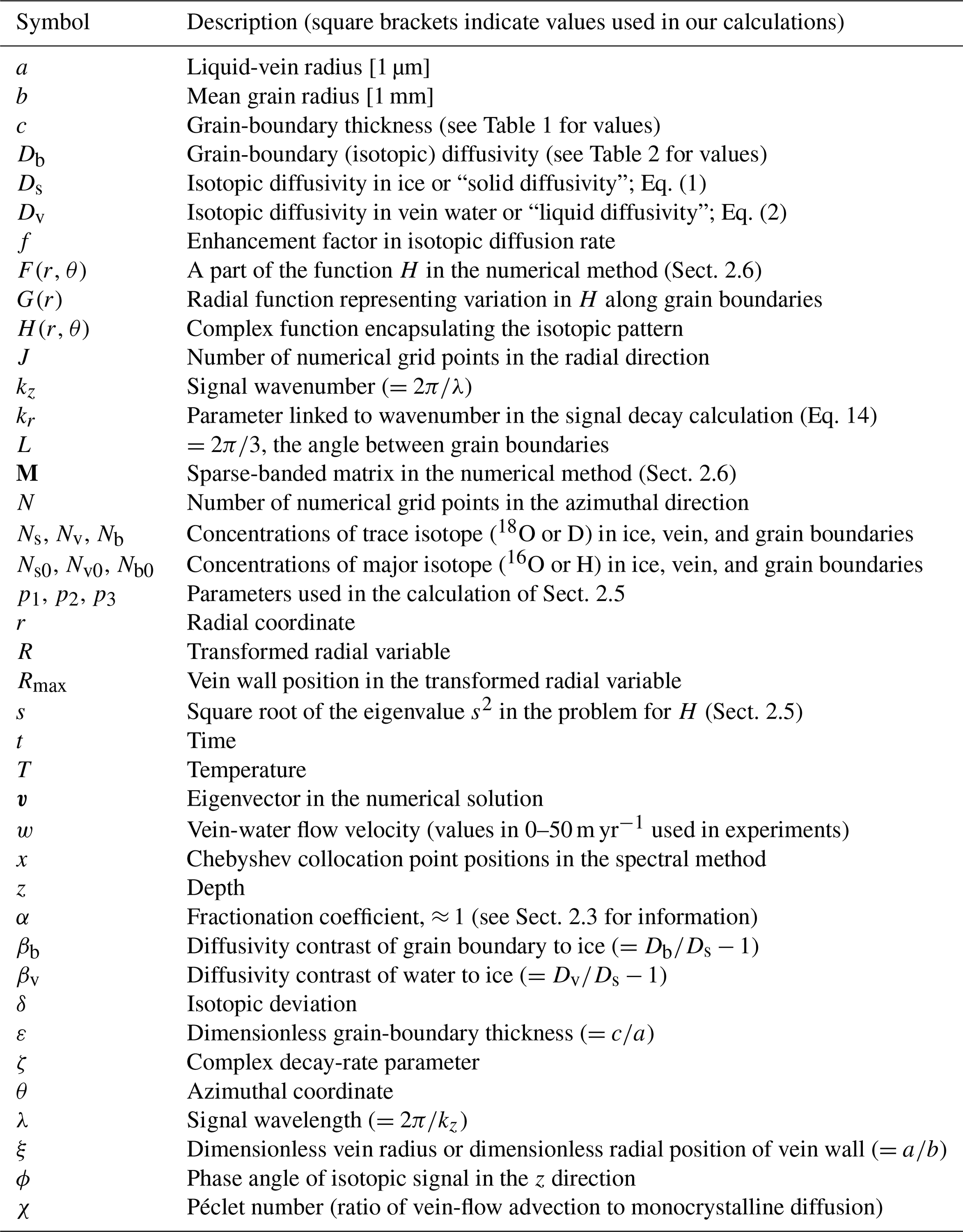
The MATLAB code for solving the model equations and computed grids of the enhancement factor are archived at https://doi.org/10.15131/shef.data.25513429 (Ng, 2024a).
Movies S1–S7 are available at https://doi.org/10.15131/shef.data.25513414 (Ng, 2024b).
The supplement related to this article is available online at: https://doi.org/10.5194/tc-18-4645-2024-supplement.
The author has declared that there are no competing interests.
Publisher’s note: Copernicus Publications remains neutral with regard to jurisdictional claims made in the text, published maps, institutional affiliations, or any other geographical representation in this paper. While Copernicus Publications makes every effort to include appropriate place names, the final responsibility lies with the authors.
I thank the City University of Hong Kong for library access during my visits, which gave me a peaceful environment for doing some of the model calculations. I acknowledge support from the University of Sheffield Institutional Open Access Fund for covering the publication cost and thank the two anonymous reviewers for their highly constructive comments on the paper. For the purpose of open access, the author has applied a Creative Commons Attribution (CC BY) licence to any author-accepted manuscript version arising from this submission.
This paper was edited by Florent Dominé and reviewed by two anonymous referees.
Árnason, B.: Equilibrium constant for the fractionation of deuterium between ice and water, J. Phys. Chem., 73, 3491–3494, 1969.
Benatov, L. and Wettlaufer, J. S.: Abrupt grain boundary melting in ice, Phys. Rev. E, 70, 061606, https://doi.org/10.1103/PhysRevE.70.061606, 2004.
BE-OI: Beyond EPICA – Oldest Ice, https://www.beyondepica.eu/en/ (last access: 9 July 2024), 2017.
Bigler, M., Svensson, A., Kettner, E., Vallelonga, P., Nielsen, M. E., and Steffensen, J. P.: Optimization of high resolution continuous flow analysis for transient climate signals in ice cores, Environ. Sci. Technol., 45, 4483–4489, https://doi.org/10.1021/es200118j, 2011.
Bohleber, P., Roman, M., Šala, M., Delmonte, B., Stenni, B., and Barbante, C.: Two-dimensional impurity imaging in deep Antarctic ice cores: snapshots of three climatic periods and implications for high-resolution signal interpretation, The Cryosphere, 15, 3523–3538, https://doi.org/10.5194/tc-15-3523-2021, 2021.
Boyd, J. P.: Chebyshev and Fourier Spectral Methods (Second Edition), Dover Publications, ISBN-13 978-0486411835, 2000.
Brox, T. I., Skidmore, M. L., and Brown, J. R.: Characterizing the internal structure of laboratory ice samples with nuclear magnetic resonance, J. Glaciol., 61, 55–64, https://doi.org/10.3189/2015JoG14J133, 2015.
Dansgaard, W.: Stable isotopes in precipitation, Tellus, 16, 436–468, https://doi.org/10.1111/j.2153-3490.1964.tb00181.x, 1964.
Dash, J. G., Rempel, A. W., and Wettlaufer, J. S.: The physics of premelted ice and its geophysical consequences, Revs. Mod. Phys., 78, 695–741, https://doi.org/10.1103/RevModPhys.78.695, 2006.
Dominé, F., Thibert, E., Van Landeghem, F., Silvente, E., and Wagnon, P.: Diffusion and solubility of HCl in ice: preliminary results, Geophys. Res. Lett., 21, 601–604, https://doi.org/10.1029/94GL00512, 1994.
Gillen, K. T., Douglass, D. C., and Hoch, M. J. R.: Self-diffusion in liquid water to −31 °C, J. Chem. Phys., 57, 5117–5119, 1972.
Gkinis, V., Simonsen, S. B., Buchardt, S. L., White, J. W. C., and Vinther, B. M.: Water isotope diffusion rates from the North-GRIP ice core for the last 16,000 years – Glaciological and paleoclimatic implications, Earth Planet. Sc. Lett., 405, 132–141,, https://doi.org/10.1016/j.epsl.2014.08.022, 2014.
Grisart, A., Casado, M., Gkinis, V., Vinther, B., Naveau, P., Vrac, M., Laepple, T., Minster, B., Prié, F., Stenni, B., Fourré, E., Steen-Larsen, H. C., Jouzel, J., Werner, M., Pol, K., Masson-Delmotte, V., Hoerhold, M., Popp, T., and Landais, A.: Sub-millennial climate variability from high-resolution water isotopes in the EPICA Dome C ice core, Clim. Past, 18, 2289–2301, https://doi.org/10.5194/cp-18-2289-2022, 2022.
Hobbs, P. V.: Ice Physics, 1st Edn., Clarendon Press, Oxford, 837 pp., ISBN 978-0198519362, 1974.
Johnsen, S. J.: Stable isotope homogenization of polar firn and ice. International Association of Hydrological Sciences Publication 118, Symposium at Grenoble 1975: Isotopes and Impurities in Snow and Ice, 210–219, 1977.
Johnsen, S. J., Clausen, H. B., Dansgaard, W., Gundestrup, N. S., Hammer, C. U., Andersen, U., Andersen, K. K., Hvidberg, C. S., Dahl-Jensen, D., Steffensen, J. P., Shoji, H.,Sveinbjörnsdóttir, Á. E., White, J., Jouzel, J., and Fisher, D.: The δ18O record along the Greenland Ice Core Project deep ice core and the problem of possible Eemian climatic instability, J. Geophys. Res.-Oceans, 102, 26397–26410, https://doi.org/10.1029/97JC00167, 1997.
Johnsen, S. J., Clausen, H. B., Cuffey, K. M., Hoffmann, G., Schwander, J., and Creyts, T.: Diffusion of stable isotopes in polar firn and ice: the isotope effect in firn diffusion, in: Physics of ice core records, edited by: Hondoh, T., Sapporo, Hokkaido University Press, 121–140, ISBN 978-4832902824, 2000.
Jones, T. R., Cuffey, K. M., White, J. W. C., Steig, E. J., Buizert, C., Markle, B. R., McConnell, J. R., and Sigl, M.: Water isotope diffusion in the WAIS Divide ice core during the Holocene and last glacial, J. Geophys. Res.-Earth, 122, 290–309, https://doi.org/10.1002/2016JF003938, 2017.
Kaufmann, P. R., Federer, U., Hutterli, M. A., Bigler, M., Schüpbach, S., Ruth, U., Schmitt, J., and Stocker, T. F.: An improved continuous flow analysis system for high-resolution field measurements on ice cores, Environ. Sci. Technol., 42, 8044–8050, https://doi.org/10.1021/es8007722, 2008.
Lehmann, M. and Siegenthaler, U.: Equilibrium oxygen- and hydrogen-isotope fractionation between ice and water, J. Glaciol., 37, 23–26, 1991.
Lu, H., McCartney, S. A., and Sadtchenko, V.: Fast thermal desorption spectroscopy study of H/D isotopic exchange reaction in polycrystalline ice near its melting point, J. Chem. Phys. 127, 184701, https://doi.org/10.1063/1.2786101, 2007.
Lu, H., McCartney, S. A., and Sadtchenko, V.: H/D exchange kinetics in pure and HCl doped polycrystalline ice at temperatures near its melting point: Structure, chemical transport, and phase transitions at grain boundaries, J. Chem. Phys., 130, 054501, https://doi.org/10.1063/1.3039077, 2009.
Lundy, T. S.: Use of the Hart–Mortlock equation to interpret tracer diffusion results, Scripta Metall. Mater, 12, 95–98, 1978.
Mader, H. M.: Observations of the water-vein system in polycrystalline ice, J. Glaciol., 38, 333–347, 1992a.
Mader, H. M.: The thermal behaviour of the water-vein system in polycrystalline ice, J. Glaciol., 38, 359–374, 1992b.
Malegiannaki, E., Peensoo, K. M., Bohleber, P., and Gkinis, V.: Challenges of water-isotope measurements on ice cores, PAGES Magazine, 31, 64–65, https://doi.org/10.22498/pages.31.2.64, 2023.
MYIC: Million Year Ice Core, https://www.antarctica.gov.au/science/climate-processes-and-change/antarctic-palaeoclimate/million-year-ice-core/ (last access: 9 July 2024), 2020.
Moreira, P. A. F. P., Veiga, R. G. D., De Almeida Ribeiro, I., Freitas, R., Helfferichf, J., and De Koning, M.: Anomalous diffusion of water molecules at grain boundaries in ice Ih, Phys. Chem. Chem. Phys., 20, 13944, https://doi.org/10.1039/c8cp00933c, 2018.
Mulvaney, R., Wolff, E. W., and Oates, K.: Sulphuric acid at grain boundaries in Antarctic ice, Nature, 331, 247–249, 1988.
Ng, F. S. L.: Pervasive diffusion of climate signals recorded in ice-vein ionic impurities, The Cryosphere, 15, 1787–1810, https://doi.org/10.5194/tc-15-1787-2021, 2021.
Ng, F. S. L.: Isotopic diffusion in ice enhanced by vein-water flow, The Cryosphere, 17, 3063–3082, https://doi.org/10.5194/tc-17-3063-2023, 2023.
Ng, F.: Numerical code of the study “The grain-scale signature of isotopic diffusion in ice”, University of Sheffield [code and data set], https://doi.org/10.15131/shef.data.25513429, 2024a.
Ng, F.: Supplement of the study “The grain-scale signature of isotopic diffusion in ice”, University of Sheffield [video], https://doi.org/10.15131/shef.data.25513414, 2024b.
Nye, J. F.: The geometry of water veins and nodes in polycrystalline ice, J. Glaciol., 35, 17–22, 1989.
Nye, J. F.: Thermal behaviour of glacier and laboratory ice, J. Glaciol., 37, 401–13, 1991.
Nye, J. F.: Diffusion of isotopes in the annual layers of ice sheets, J. Glaciol., 44, 467–468, 1998.
Nye, J. F. and Frank, F. C.: Hydrology of the intergranular veins in a temperate glacier, International Association of Scientific Hydrology Publication 95, Symposium at Cambridge 1969 – Hydrology of Glaciers, 157–161, 1973.
O'Neil, J. R.: Hydrogen and oxygen isotope fractionation between ice and water, J. Phys. Chem., 72, 3683–3684, 1968.
Pol, K., Masson-Delmotte, V., Johnsen, S., Bigler, M., Cattani, O., Durand, G., Falourd, S., Jouzel, J., Minster, B., Parrenin, F., Ritz, C., Steen-Larsen, H. C., and Stenni, B.: New MIS 19 EPICA Dome C high resolution deuterium data: Hints for a problematic preservation of climate variability at sub-millennial scale in the “oldest ice”, Earth Planet. Sc. Lett., 298, 95–103, https://doi.org/10.1016/j.epsl.2010.07.030, 2010.
Prielmeier, F. X., Lang, E. W., Speedy, R. J., and Lüdemann, H.-D.: The pressure dependence of self diffusion in supercooled light and heavy water, Ber. Bunsenges. Phys. Chem., 92, 1111–1117, 1988.
Ramseier, R. O.: Self-diffusion of tritium in natural and synthetic ice monocrystals, J. Appl. Phys., 38, 2553–2556, 1967.
Rempel, A. W. and Wettlaufer, J. S.: Isotopic diffusion in polycrystalline ice, J. Glaciol., 49, 397–406, 2003.
Steig, E. J., Jones, T. R., Schauer, A. J., Kahle, E. C., Morris, V. A., Vaughn, B. H., Davidge, L., and White, J. W. C.: Continuous-flow analysis of δ17O, δ18O, and δD of H2O on an ice core from the South Pole, Front. Earth Sci., 9, 640292, https://doi.org/10.3389/feart.2021.640292, 2021.
Stoll, N., Bohleber, P., Dallmayr, R., Wilhelms, F., Barbante, C., and Weikusat, I.: The new frontier of microstructural impurity research in polar ice, Ann. Glaciol., 1–4, https://doi.org/10.1017/aog.2023.61, online first, 2023.
Thibert, E. and Dominé, F.: Thermodynamics and kinetics of the solid solution of HCl in ice, J. Phys. Chem. B., 101, 3554–3565, https://doi.org/10.1021/jp962115o, 1997.
Thomson, E. S., Hansen-Goos, H., Wettlaufer, J. S., and Wilen, L. A.: Grain boundary melting in ice, J. Chem. Phys., 138, 124707, https://doi.org/10.1063/1.4797468, 2013.
Trefethen, L. N.: Spectral methods in MATLAB, Society for Industrial and Applied Mathematics (SIAM), ISBN 0-89871-465-6, 2000.
Vinther, B. M., Clausen, H. B., Johnsen, S. J., Rasmussen, S. O., Andersen, K. K., Buchardt, S. L., Dahl-Jensen, D., Seierstad, I. K., Siggaard-Andersen, M-L., Steffensen, J. P., Svensson, A., Olsen, J., and Heinemeier, J.: A synchronized dating of three Greenland ice cores throughout the Holocene, J. Geophys. Res., 113, D13102, https://doi.org/10.1029/2005JD006921, 2006.
Wettlaufer, J. S.: Impurity effects in the premelting of ice, Phys. Rev. Letts., 82, 2516–2519, 1999.
Whillans, I. M. and Grootes, P. M: Isotopic diffusion in cold snow and firn, J. Geophys. Res., 90, 3910–3918, https://doi.org/10.1029/JD090iD02p03910, 1985.
Xu, Y., Petrika, N. G., Smith, R. S., Kay, B. D., and Kimmel, G. A.: Growth rate of crystalline ice and the diffusivity of supercooled water from 126 to 262 K, P. Natl. Acad. Sci. USA, 113, 14921–14925, https://doi.org/10.1073/pnas.1611395114, 2016.
Yagasaki, T., Matsumoto, M., and Tanaka, H.: Molecular dynamics study of grain boundaries and triple junctions in ice, J. Chem. Phys., 153, 124502, https://doi.org/10.1063/5.0021635, 2020.
That the Hart–Mortlock equation may only roughly approximate the bulk/effective diffusivity in some applications has been recognised (e.g. Lundy, 1978). Moreover, for the coupled diffusion studied here, our results (Sect. 3.2) imply a bulk diffusivity varying with signal wavelength, not what the Hart–Mortlock equation would predict.
We have not found published values of α (for the liquid–solid phase change) in T<0, certainly not at −32 and −52 °C. It is unsurprising that laboratory measurements of α have not been made at the strongly depressed melting temperatures specific to the vein system.
Mathematically, λ≫b (dimensionally) translates to kz≪1 and p1≪1 in the scaled model of Sect. 2.4 and 2.5 so that Eqs. (22) to (25) for H approximate a boundary value problem with terms representing vertical gradients neglected. Near where the isotopic pattern changes polarity, this approximation breaks down because H≈0 and those terms become comparable to the radial and azimuthal gradients.
Our computed surfaces at low Db differ from Fig. 12a and e negligibly and could equally serve as the references.