Modelling the effect of free convection on permafrost melting rates in frozen rock clefts

This research develops a conceptual model of a karst system subject to mountain permafrost. The transient thermal response of a frozen rock cleft after the rise in the atmospheric temperature above the melting temperature of water is investigated using numerical simulations. Free convection in liquid water (i.e. buoyancy-driven flow) is considered. The density increase in water from 0 to 4 °C causes warmer meltwater to flow downwards and colder upwards, resulting in significant enhancement of the heat transferred from the ground surface to the melting front. Free convection increases the melting rate by approximately an order of magnitude compared to a model based on thermal conduction in stagnant water. The model outcomes are compared qualitatively with field data from the Monlesi ice cave (Switzerland) and confirm the agreement between real-world observations and the proposed model when free convection is considered.

1 Introduction

With global climate change and rising temperatures, permafrost degradation has become a significant concern (Duvillard et al., 2021; Walvoord and Kurylyk, 2016; Jin et al., 2021). This is particularly true in mountainous regions where rapid thawing causes subsidence and rockfalls that impact construction work and tourist facilities (Haeberli et al., 2017). Thawing permafrost poses serious challenges to infrastructure built on frozen ground, including buildings, roads, pipelines, and railways (Larsen et al., 2008; Cheng, 2005; Pham et al., 2008; Zhang et al., 2005; Fortier et al., 2011). Permafrost acts as a natural barrier, preventing water from infiltrating into the ground. As it thaws, drainage patterns are altered, leading to increased erosion and discharge of groundwater into rivers and lakes (Bense et al., 2012; Andresen et al., 2020; Fabre et al., 2017; Painter et al., 2016; Walvoord and Kurylyk, 2016). Permafrost degradation can also disrupt ecosystems adapted to frozen conditions. Trees, plants, and wildlife that rely on permafrost stability may struggle to adapt to climate changes, leading to shifts in species distribution and ecosystem dynamics depending on the permafrost melting rate (Hayward et al., 2018; Krumhansl et al., 2015; Pelletier et al., 2018).

Field measurements in boreholes (e.g. Noetzli et al., 2021; Haberkorn et al., 2021) and caves (Luetscher et al., 2008; Colucci and Guglielmin, 2019; Wind et al., 2022) have shown that heat advected by water and air fluxes may significantly disturb the geothermal field, challenging classical models of heat propagation based on conductive fluxes. In carbonate environments in particular, the infiltration of water along well-developed conduits may produce a thermal anomaly deep into the karst system. The discontinuous nature of permafrost in karst environments may lead to the formation of massive cave ice at depth (Bartolomé et al., 2022) but may also explain unexpected speleothem formations during glacial times (Luetscher et al., 2015; Fohlmeister et al., 2023).

Efforts are being made to study and understand permafrost degradation to mitigate its impacts. So far, most studies have considered mainly conductive and latent heat fluxes (Malakhova, 2022; Galushkin, 1997; Ivanov and Rozhin, 2022; Marchenko et al., 2008; Schuster et al., 2018; Jafarov et al., 2012; Cicoira et al., 2019; Hornum et al., 2020). Such models are, however, not applicable to heterogeneous, ice-rich media including debris slopes, rock glaciers, and fractured and/or karst aquifers. But, even though conventional 1D transient models are not suitable for every context, they offer several advantages, including lower computational costs than 2D or 3D models and easy implementation. Pruessner et al. (2021) investigated glacier runoff associated with permafrost degradation in high-Alpine catchments. They used two different methods: GERM (Huss et al., 2008) and SNOWPACK (Bartelt and Lehning, 2002), which are based on 1D transient conduction considering latent heat exchanges, different thermal properties of ground layer constituents, and ventilation effects. This distributed model is efficient for the calculation of temperature in large domains (catchment scale). Mohammed et al. (2021) developed a hydro–thermal–solutal model for analysing reactive solute transport in a permafrost-affected groundwater system by considering convective flux in the energy balance. Tubini et al. (2021) proposed a numerical approach for modelling heat transfer of permafrost thawing based on conduction and latent heat flux in a 1D domain that is capable of dealing with high time steps and maintains conservation of energy in long-term simulations. Hasler et al. (2011) built a conceptual model combining numerical modelling and laboratory experiments to investigate the effect of advective heat transport induced by water drainage in frozen rock clefts and fractures at small scales. They built a conceptual model combining numerical modelling and laboratory experiments. These authors find a significant effect of water flow inside the clefts, due to the formation of thermal shortcuts between the atmosphere and the subsurface.

Although the majority of these studies are designed to address large-scale problems, they typically neglect free convection within the liquid water phase. This process could nonetheless play an important role in the total heat transfer, particularly in geographically restricted areas subject to mountain permafrost (Haberkorn et al., 2021). Figure 1a displays the bottom of a frozen cleft hosted in Alpine karst. Such clefts and fissures are characterised by distinct geometries accommodating contrasting volumes of ice. Our aim is to study the effect of free convection on the melting rate in frozen rock clefts and/or karst conduits at the daily scale. Atmospheric warming at the upper boundary melts the ice from the top of the fractures and increases the meltwater temperature. While most fluids expand as temperature increases, liquid water shrinks when warmed from 0 to 4 °C (see the maximum density at 4 °C in Fig. 2). Therefore, the progressive warming of the meltwater at the top of the cleft results in an unstable situation (heavier fluid above lighter) that triggers free convection (buoyancy-driven flow). To assess the thermal reaction time and thus the hydrological breakthrough associated with the thawing of mountain permafrost, we model the heat exchange in a frozen rock cleft. We assess the temperature field in the meltwater, ice, and surrounding rock by numerical simulations, as well as the velocity field within the liquid water, to elucidate the main mechanisms driving the thawing of ice. Although physical monitoring of such processes is hardly possible, our model fits as closely as possible to effective field observations. A systematic comparison is conducted under similar thermal settings for two cases: one that considers heat conduction in stagnant liquid water (SLW) and the second where free convection (FC) is taken into account. Our study shows how free convection enhances the melting rate of an ice cleft at different aperture sizes.

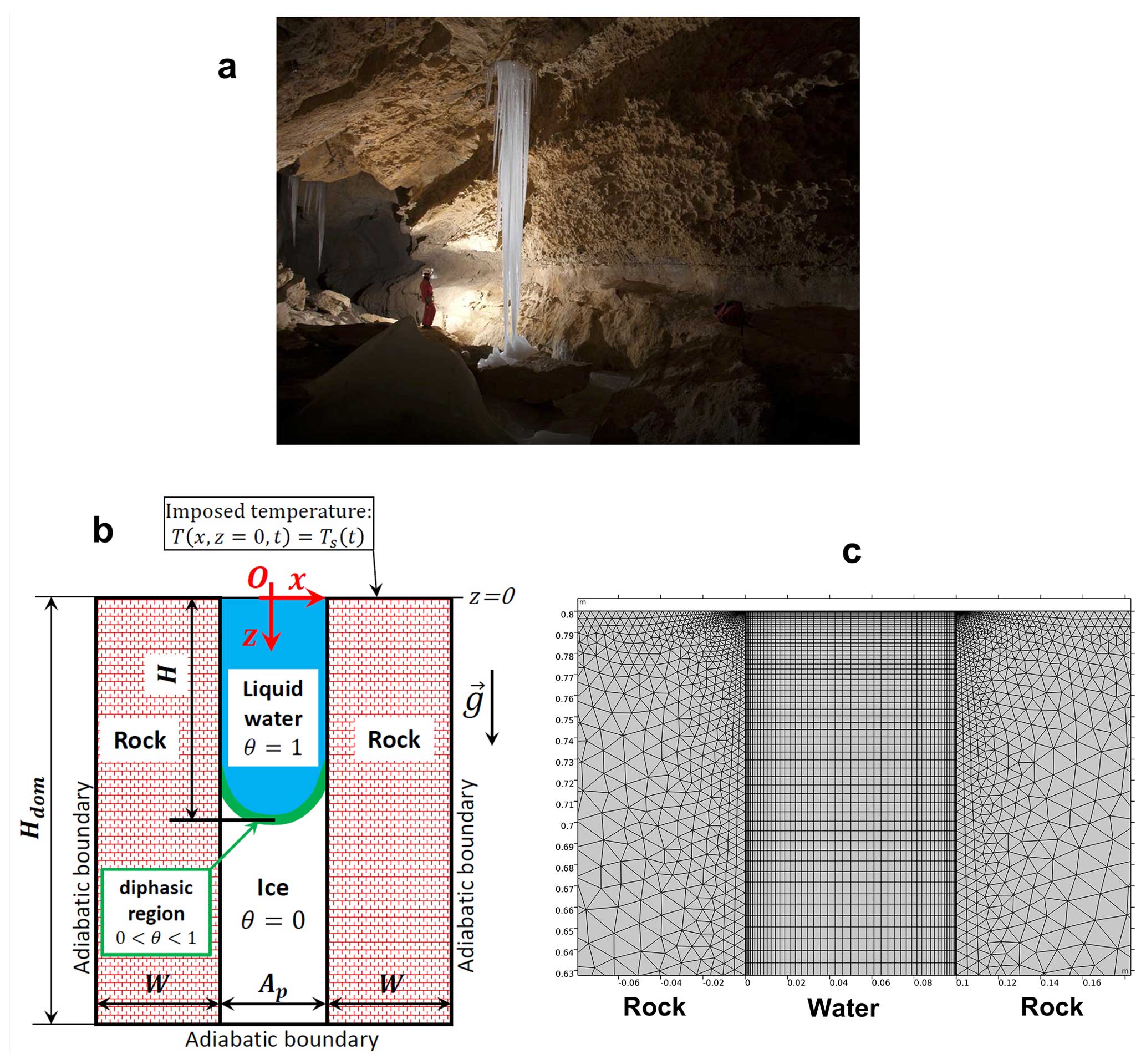
Figure 1 (a) Pingouins cave, Switzerland, showing ice-filled clefts exposed on the cave roof (photo courtesy of Arnaud Conne). (b) Computational domain with external boundary conditions ($\mathrm{2}\mathrm{cm}\le A_p\le \mathrm{50}\mathrm{cm}$, H_dom=0.8 m, and W_dom=1 m; the sketch is not to scale). (c) Finite element mesh in the upper part of the computational domain.

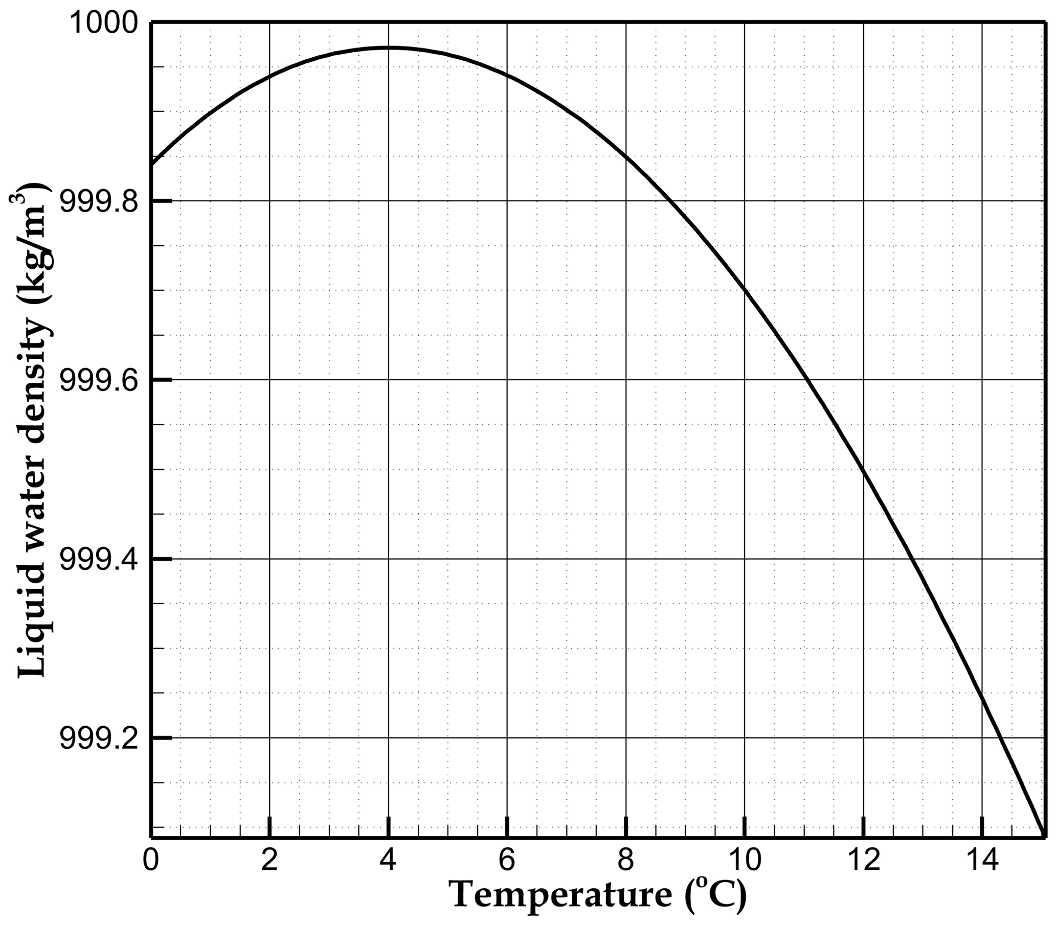
Figure 2 Density of liquid water as a function of temperature (produced using Comsol Multiphysics).

2 Computational domain and governing equations

2.1 Physical model and simplifying assumptions

We consider the upper part of a single vertical cleft of size aperture A_p filled with pure water whose melting point is T_m=0 °C. This cleft is surrounded by a rock mass of width W (see Fig. 1b). In karst massifs, water flow concentrates in well-defined conduits (Ford and Williams, 2007). The micro-porosity of the rock is thus disregarded, and impermeable rock mass is assumed.

The cleft is located at the centre of the 2D domain of height H_dom. In the initial state, the system (water and surrounding rock) is at the uniform initial temperature $T_{\mathrm{i}}=-\mathrm{1}$ °C, and all the water is frozen. At time t=0, the temperature of the ground surface T_s increases at the constant rate of 1.77 °C h⁻¹ to reach 15 °C after 9 h. This temperature increase is similar to the daily warming between the early morning and the afternoon.

The effect of the cleft aperture size was investigated by varying A_p from 2 to 50 cm. We imposed H_dom=0.8 m and W=1 m in all simulations. These values are large enough such that the thermal perturbation induced by the presence of the cleft does not reach the domain boundaries by the end of the simulated time (9 h). The vertical and bottom boundaries of the domain can therefore be considered adiabatic (see Fig. 1b). It is important to note that the domain height H_dom contains only the upper part of the cleft, whose actual depth commonly ranges from 1 to 10 m. The value of H_dom used in this study is convenient for the daily timescale considered in the numerical simulations. Simulating larger timescales would require larger values of H_dom.

2.2 Governing equations

The temperature T is the only dependent variable in the impermeable rock domain. It satisfies the standard heat equation,

$$\begin{array}{}\text{(1)}& {\mathit{\rho }}_{\mathrm{r}}{c}_{p,\mathrm{r}}{\displaystyle \frac{\partial T}{\partial t}}=k_{\mathrm{r}}\left({\displaystyle \frac{{\partial }^{\mathrm{2}}T}{\partial x^{\mathrm{2}}}}+{\displaystyle \frac{{\partial }^{\mathrm{2}}T}{\partial z^{\mathrm{2}}}}\right),\end{array}$$

where ρ_r, c_p,r, and k_r are the rock density, specific heat, and thermal conductivity, respectively. z is the depth and x the horizontal distance from the symmetry plane of the cleft (see Fig. 1b).

The water domain is more intricate. The velocity field must be calculated in the liquid part of the domain but reduces to zero in the frozen region. To avoid the difficult task of tracking the moving boundary between ice and liquid water, we adopted a strategy that allows us to define the same set of dependent variables and governing equations in the entire water domain. To this end, we perform the approximation of smooth phase transition between solid and liquid phases. We assume that ice melting begins at temperature $T_{\text{m1}}=T_{\mathrm{m}}-\mathrm{\Delta }T$ and ends at $T_{\text{m2}}=T_{\mathrm{m}}+\mathrm{\Delta }T$ (water is in solid state for T<T_m1, in liquid state for T<T_m2, and both phases coexist for $T_{\text{m1}}\le T\le T_{\text{m2}}$). It is important to note that in this study, ΔT is a numerical parameter with no physical meaning. Ideally, the behaviour of a pure substance melting at temperature T_m is recovered for ΔT→0. Decreasing ΔT thus improves the model accuracy but requires more computational resources (see Michałek and Kowalewski, 2003; Zeneli et al., 2019; Bourdillon et al., 2015; and Arosemena, 2018, for more details). In practice, the setting of ΔT results from a sensitivity analysis. Its value must be decreased until it does not change the results. This is the purpose of Appendix A, where it is shown that the model is a good approximation of a pure substance for ΔT≤0.7 °C.

The dependent variables defined in the water domain are the temperature T, the horizontal and vertical components of the velocity vector u and v, the pressure p, and the liquid volume fraction θ. Because of the assumption of smooth phase transition, θ varies continuously from 0 (solid phase) to 1 (liquid phase) throughout the water domain (see Fig. 1b). The corresponding governing equations read

$$\begin{array}{}\text{(2)}& {\displaystyle \frac{\partial u}{\partial x}}+{\displaystyle \frac{\partial v}{\partial z}}=\mathrm{0}\text{(3)}& {\displaystyle }\begin{array}{rl}{\displaystyle }{\mathit{\rho }}_{\mathrm{0}}{\displaystyle \frac{\partial u}{\partial t}}& {\displaystyle }+{\mathit{\rho }}_{\mathrm{0}}\left(u{\displaystyle \frac{\partial u}{\partial x}}+v{\displaystyle \frac{\partial u}{\partial z}}\right)=\\ {\displaystyle }& {\displaystyle }-{\displaystyle \frac{\partial p}{\partial x}}+\mathit{\mu }\left({\displaystyle \frac{{\partial }^{\mathrm{2}}u}{\partial x^{\mathrm{2}}}}+{\displaystyle \frac{{\partial }^{\mathrm{2}}u}{\partial z^{\mathrm{2}}}}\right)+A{\displaystyle \frac{(\mathrm{1}-\mathit{\theta }{)}^{\mathrm{2}}}{{\mathit{\theta }}^{\mathrm{3}}+\mathit{\epsilon }}}u\end{array}\text{(4)}& {\displaystyle }\begin{array}{rl}{\displaystyle }{\mathit{\rho }}_{\mathrm{0}}{\displaystyle \frac{\partial v}{\partial t}}& {\displaystyle }+{\mathit{\rho }}_{\mathrm{0}}\left(u{\displaystyle \frac{\partial v}{\partial x}}+v{\displaystyle \frac{\partial v}{\partial z}}\right)=\\ {\displaystyle }& {\displaystyle }-{\displaystyle \frac{\partial p}{\partial z}}+\mathit{\mu }\left({\displaystyle \frac{{\partial }^{\mathrm{2}}v}{\partial x^{\mathrm{2}}}}+{\displaystyle \frac{{\partial }^{\mathrm{2}}v}{\partial z^{\mathrm{2}}}}\right)-{\mathit{\rho }}_{\mathrm{0}}g\mathit{\beta }(T-T_{\mathrm{0}})\\ {\displaystyle }& {\displaystyle }+{\mathit{\rho }}_{\mathrm{0}}g+A{\displaystyle \frac{(\mathrm{1}-\mathit{\theta }{)}^{\mathrm{2}}}{{\mathit{\theta }}^{\mathrm{3}}+\mathit{\epsilon }}}v\end{array}\text{(5)}& {\displaystyle }\mathit{\rho }{c}_p{\displaystyle \frac{\partial T}{\partial t}}+\mathit{\rho }{c}_p\left(u{\displaystyle \frac{\partial T}{\partial x}}+v{\displaystyle \frac{\partial T}{\partial z}}\right)-k\left({\displaystyle \frac{{\partial }^{\mathrm{2}}T}{\partial x^{\mathrm{2}}}}+{\displaystyle \frac{{\partial }^{\mathrm{2}}T}{\partial z^{\mathrm{2}}}}\right)=\mathrm{0}\text{(6)}& {\displaystyle }\mathit{\theta }=\left\{\begin{array}{ll}\mathrm{0}& T<T_{\text{m1}}\left(\text{solid}\right)\\ {\displaystyle \frac{T-T_{\text{m1}}}{T_{\text{m2}}-T_{\text{m1}}}}& T_{\text{m1}}\le T\le T_{\text{m2}}\left(\text{diphasic}\right)\\ \mathrm{1}& T>T_{\text{m2}}\left(\text{liquid}\right).\end{array}\right.\end{array}$$

This set of equations includes mass balance (Eq. 2), momentum balance (Eqs. 3 and 4), energy balance (Eq. 5), and the relation between the liquid volume fraction θ and the temperature field (Eq. 6). g is the gravity acceleration; ρ₀ is the density of liquid water at the reference temperature T₀; μ and β are the dynamic viscosity and thermal expansion coefficient of liquid water; and ρ, c_p, and k are the density, specific heat, and thermal conductivity of water.

The last term in Eqs. (3) and (4) is used to impose the velocity transition between the liquid and solid phases. A and ε are numerical parameters imposed by the user. A must be as large as possible, provided that solver stability is insured. In contrast, ε is a small parameter used to prevent divisions by zero in numerical calculations (Mousavi Ajarostaghi et al., 2019). It can be demonstrated that for θ=0 (i.e. in the solid phase), the solution of Eqs. (2) and (4) turns to $u\simeq v\simeq \mathrm{0}$, which is the solution expected in the solid phase (see Nazzi Ehms et al., 2019, and Caggiano et al., 2018, for more details). Conversely, the last term in Eqs. (3) and (4) vanishes for θ=0 (i.e. in the liquid phase). In this case, Eqs. (3) and (4) turn into the standard Navier–Stokes equations (momentum balance in an incompressible Newtonian fluid) required to calculate the velocity field in the liquid phase.

The boundary conditions are as follows. At the interface between an impermeable solid and a viscous fluid, the fluid velocity is equal to that of the solid (Guyon et al., 2015). These are the so-called no-slip and impermeability conditions, resulting in $u=v=\mathrm{0}$ at the rock–water interface. The temperature continuity and the heat flux conservation through this interface are also considered (since the water velocity vanishes at the rock–water interface, the heat flux through the interface reduces to conduction). As already mentioned in Sect. 2.1, the bottom and vertical external boundaries are adiabatic, and the temperature evolution of the top boundary T_s increases at a constant rate (see Fig. 1b).

2.3 Material properties

The physical properties used in the simulations are listed in Table 1. Subscripts “r”, “s”, and “l” refer to rock, ice, and liquid water, respectively. No subscript indicates the effective physical properties considered in the governing equations of the water domain (solid, liquid, and diphasic). They are estimated from the liquid volume fraction θ as follows:

$$\begin{array}{}\text{(7)}& {\displaystyle }\mathit{\rho }={\mathit{\rho }}_{\mathrm{s}}(\mathrm{1}-\mathit{\theta })+{\mathit{\rho }}_{\mathrm{l}}\mathit{\theta }\text{(8)}& {\displaystyle }k=k_{\mathrm{s}}(\mathrm{1}-\mathit{\theta })+k_{\mathrm{l}}\mathit{\theta }\text{(9)}& {\displaystyle }\begin{array}{rl}{\displaystyle }{c}_p& {\displaystyle }={\displaystyle \frac{{\mathit{\rho }}_{\mathrm{s}}{c}_{p,\mathrm{s}}(\mathrm{1}-\mathit{\theta })+{\mathit{\rho }}_{\mathrm{l}}{c}_{p,\mathrm{l}}\mathit{\theta }}{\mathit{\rho }}}+L_{\mathrm{m}}{\displaystyle \frac{\partial {\mathit{\alpha }}_{\mathrm{m}}}{\partial T}}\mathrm{\text{with}}\\ {\displaystyle }& {\displaystyle }{\mathit{\alpha }}_{\mathrm{m}}={\displaystyle \frac{\mathrm{1}}{\mathrm{2}}}{\displaystyle \frac{{\mathit{\rho }}_{\mathrm{l}}\mathit{\theta }-{\mathit{\rho }}_{\mathrm{s}}(\mathrm{1}-\mathit{\theta })}{{\mathit{\rho }}_{\mathrm{l}}\mathit{\theta }+{\mathit{\rho }}_{\mathrm{s}}(\mathrm{1}-\mathit{\theta })}}\end{array}\text{(10)}& {\displaystyle }\mathit{\mu }={\mathit{\mu }}_{\mathrm{l}}.\end{array}$$

The effective specific heat c_p defined in Eq. (9) takes into account the latent heat of melting L_m.

Table 1 Thermal properties and numerical parameters. The liquid water properties are temperature dependent. The properties of ice and rock are assumed to be constant.

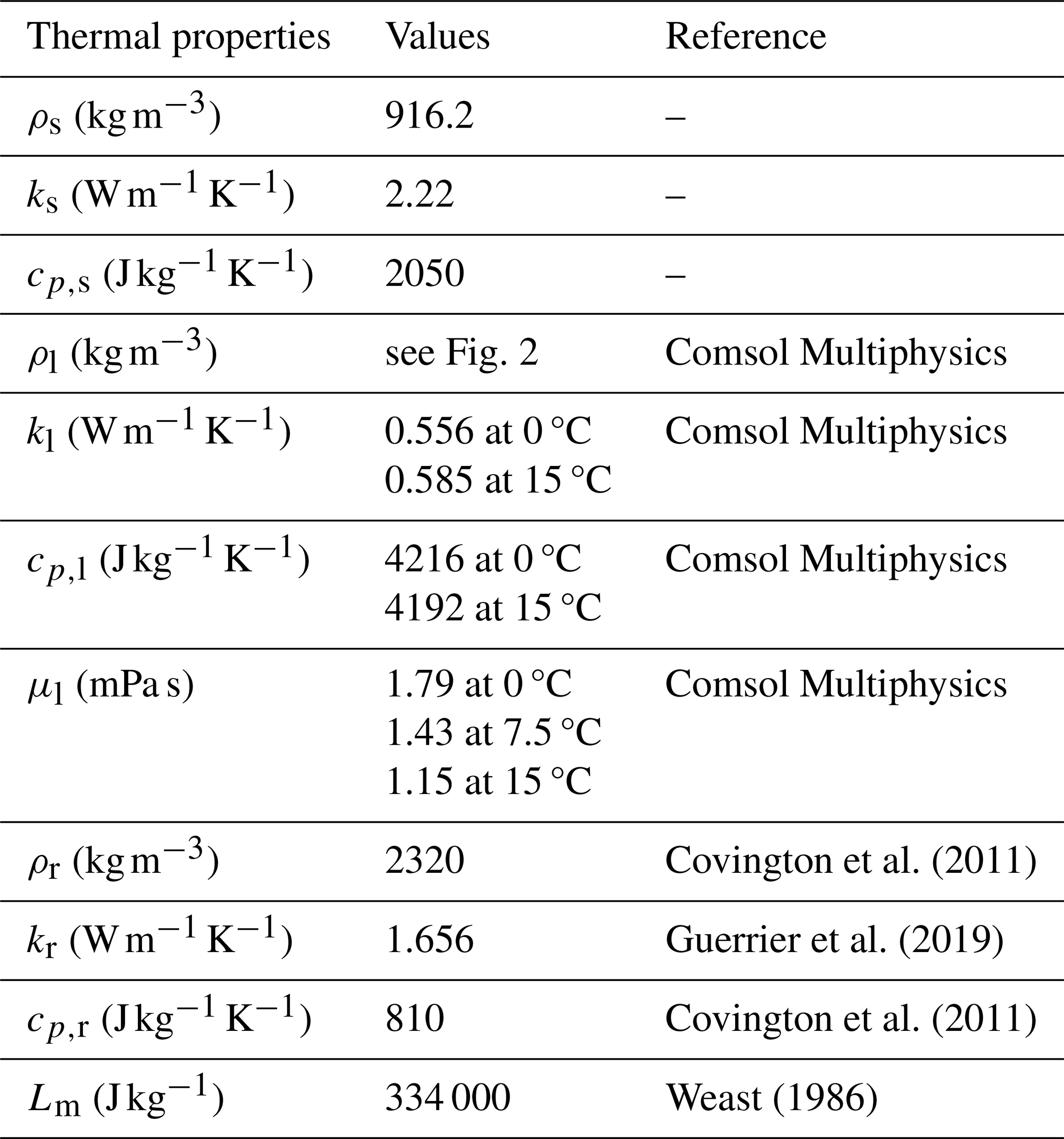
The standard Boussinesq approximation is assumed in the liquid phase (Spiegel and Veronis, 1960; Bejan, 2013). This approximation, widely used for free-convection modelling, consists of assuming constant liquid density in the governing equations (Eqs. 2, 3, and 4), except in the buoyancy term of the momentum balance equations (Eqs. 3 and 4). The thermal expansion coefficient β at the origin of buoyancy is estimated from the relation

$$\begin{array}{}\text{(11)}& \mathit{\beta }=-{\displaystyle \frac{\mathrm{1}}{{\mathit{\rho }}_{\mathrm{l}}}}{\displaystyle \frac{\mathrm{d}{\mathit{\rho }}_{\mathrm{l}}}{\mathrm{d}T}},\end{array}$$

where ρ_l is the temperature-dependent liquid water density displayed in Fig. 2 (the order of magnitude of β in the unstable temperature range from 0 to 4 °C is approximately $-\mathrm{3}\times {\mathrm{10}}^{-\mathrm{5}}$ K⁻¹). In contrast, the constant liquid density ρ₀ estimated at the reference temperature T₀ is considered in the inertia terms of Eqs. (3) and (4) (ρ₀=999.84 kg m⁻³ at T₀=0 °C). The Boussinesq approximation is valid if the maximum fluid density variation Δρ_l is much lower than the liquid density ρ_l, a condition usually satisfied in liquids ($\mathrm{\Delta }{\mathit{\rho }}_{\mathrm{l}}/{\mathit{\rho }}_{\mathrm{l}}\sim {\mathrm{10}}^{-\mathrm{3}}$ in our case).

The density of water is greater than that of ice by approximately 10 %. This induces a reduction in volume upon melting that is neglected in our model. This is equivalent to assuming that an external water flow replenishes the top layer of the domain with water at the ground surface temperature T_s. This would result in additional vertical velocity in the liquid phase (Heitz and Westwater, 1970):

$$\begin{array}{}\text{(12)}& v_{\mathrm{l}}={\displaystyle \frac{\left({\mathit{\rho }}_{\mathrm{l}}-{\mathit{\rho }}_{\mathrm{s}}\right)}{{\mathit{\rho }}_{\mathrm{l}}}}{\displaystyle \frac{\mathrm{d}H}{\mathrm{d}t}}.\end{array}$$

This velocity would be that of the liquid in the absence of free convection or would be added to the free-convection velocity field in the other case. This contraction-induced flow can be neglected if the heat advected in that way is negligible compared to the heat absorbed by the motion of the melting front:

$$\begin{array}{}\text{(13)}& {\mathit{\rho }}_{\mathrm{l}}{v}_{\mathrm{l}}{c}_{\text{pl}}(T_{\mathrm{s}}-T_{\mathrm{m}})\ll L_{\mathrm{m}}{\mathit{\rho }}_{\mathrm{s}}{\displaystyle \frac{\mathrm{d}H}{\mathrm{d}t}}.\end{array}$$

Equations (12) and (13) yield the condition of validity:

$$\begin{array}{}\text{(14)}& {\displaystyle \frac{\left({\mathit{\rho }}_{\mathrm{l}}-{\mathit{\rho }}_{\mathrm{s}}\right)}{{\mathit{\rho }}_{\mathrm{s}}}}{\displaystyle \frac{c_{\text{pl}}(T_{\mathrm{s}}-T_{\mathrm{m}})}{L_{\mathrm{m}}}}\ll \mathrm{1}.\end{array}$$

With the physical properties of Table 1 and $T_{\mathrm{s}}-T_{\mathrm{m}}=\mathrm{15}$ °C, the left-hand side of Eq. (14) is approximately equal to 0.02, much lower than 1. The volume change induced by melting can thus be safely neglected. Heitz and Westwater (1970) presented a comparison of mathematical solutions with equal and unequal phase densities. In a configuration close to ours, they showed that considering equal densities for ice and liquid water resulted in a negligible loss of accuracy.

2.4 Numerical methods

The system of partial differential equations (Eqs. 1–6) was solved using finite elements with the software Comsol Multiphysics version 6.0 (Galerkin method with quadratic Lagrangian elements, time discretisation by implicit backward differentiation formula).

The mesh density close to the walls was refined due to the high gradient of velocity, and a structured (mapped) mesh type was used for the water–ice domain, as shown in Fig. 1c. The mesh was validated by a sensitivity analysis comparing four different mesh qualities, with 14 000, 24 000, 32 000, and 47 000 elements, respectively. The difference in the results between the latter three cases was found to be insignificant. The mesh with 24 000 elements was thus selected in all simulations.

Regarding the numerical parameters required to model melting, we imposed ΔT=0.5 °C, A=1000 $\mathrm{kg}{\mathrm{m}}^{-\mathrm{3}}{\mathrm{s}}^{-\mathrm{1}}$, and $\mathit{\epsilon }={\mathrm{10}}^{-\mathrm{3}}$. We checked that imposing ΔT=0.3 or 0.7 °C did not significantly change the results (see Appendix A). The selected values of A and ε produced vanishingly small velocity fields in the ice, with no deterioration of the solver stability.

3 Model validation

The validity of our model is tested by comparison with two studies from the literature. A simple test case assuming stagnant liquid water (no free convection) was selected as a first step (numerical simulation of ice freezing by Kahraman et al., 1998). In a second step, our model was tested against experimental results including free convection (ice melting experiment by Virag et al., 2006).

3.1 Stagnant liquid water

When free convection is neglected, conduction and latent heat fluxes are the only mechanisms transferring heat in liquid water and ice. We compare our results with the results from Kahraman et al. (1998). These authors developed a model to examine the heat transfer of ice melting inside a 20 cm×20 cm square, assuming stagnant liquid water. A brief description of their conceptual model is given in Fig. 3a. Ice is at an initial temperature of −30 °C and is exposed to a temperature of 20 °C over half of the lower boundary ($\mathrm{0}\le x\le \mathrm{10}\mathrm{cm}$, y=0 cm) and 70 °C over the other half ($\mathrm{10}\le x\le \mathrm{20}\mathrm{cm}$, y=0 cm). The temperature of the solid ice at the top boundary (y=20 cm) is maintained at 0 °C, and the other surfaces (left and right sides) are insulated (Fig. 3a). Figure 3b shows the temperature distribution after 5 h modelled in the present work. Temperature profiles at x=4 and x=16 cm at different times of melting can be seen in Fig. 3c and d, respectively. The result of our model is in good agreement with Kahraman et al. (1998).

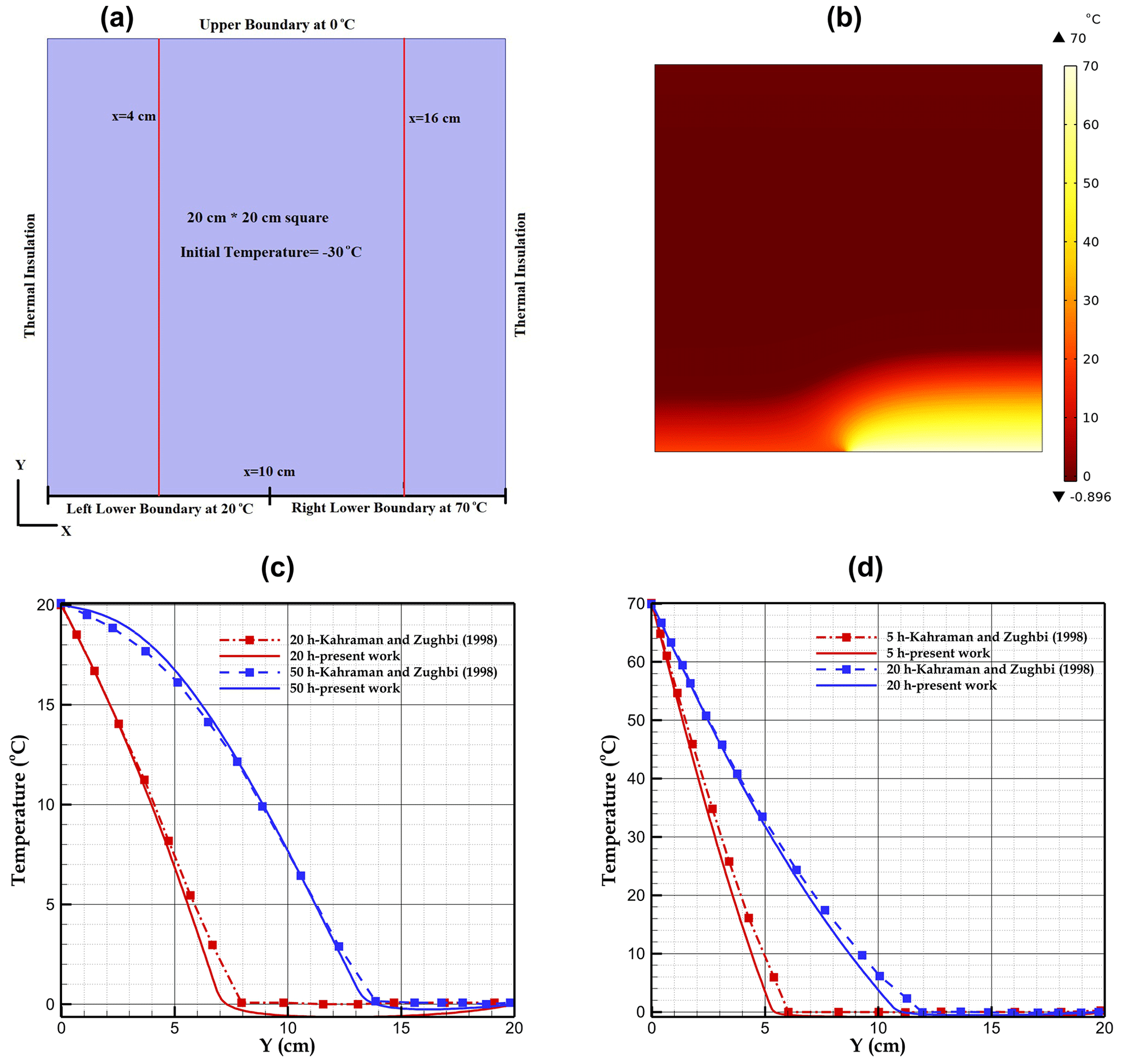
Figure 3 (a) Model geometry including initial and boundary conditions, (b) the contour of temperature at t=5 h, and the temperature profile of ice and water at different times of ice melting at (c) x=4 cm and (d) x=16 cm.

3.2 Free convection

Virag et al. (2006) investigated the effect of free convection on ice melting inside a cavity with an experimental approach shown in Fig. 4a. The lower and top surfaces are thermally insulated. The left and right boundaries are at 0 and 8 °C, respectively. Figure 4b displays the contours of temperature (left) and the velocity field, as well as the velocity vectors (right) predicted by our model. The black arrows indicate the direction of the water flow. The model predicts the existence of two contra-rotating free-convection cells separated by the 4 °C isotherm, which corresponds to the maximum liquid water density. In the small cell located in the lower-left corner, where temperature is higher than 4 °C, the liquid rises upward along the warm wall, as expected when the liquid density is a decreasing function of temperature. In the bigger cell located in the upper part of the liquid region, where the temperature is less than 4 °C, the warmer liquid moves downward, as expected when the liquid density increases with temperature. Furthermore, results show that where the temperature gradient is high, the magnitude of the local velocity increases. This is seen next to the left boundary and also close to the ice interface. The convection-induced mixing homogenises the temperature in the liquid phase.

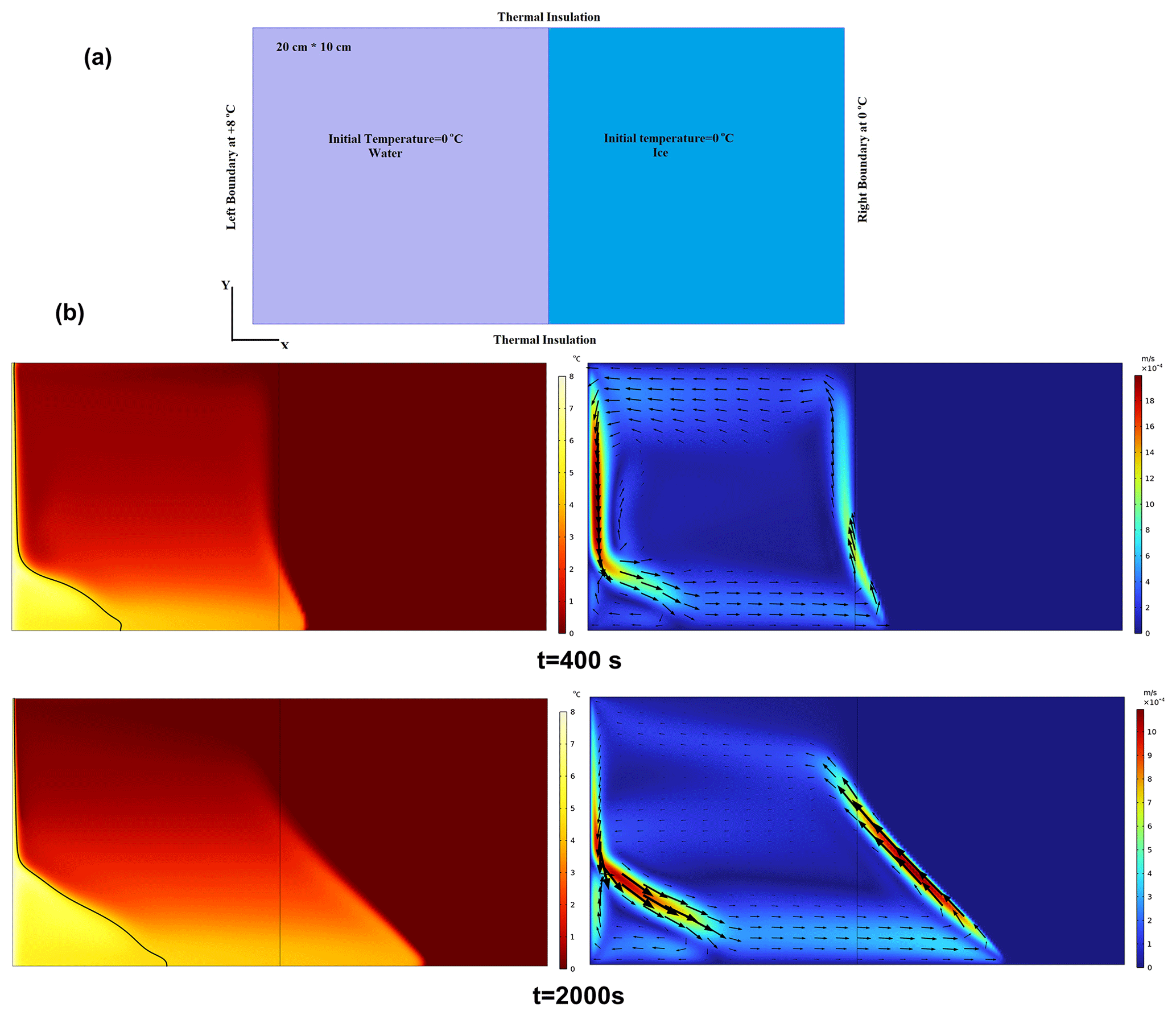
Figure 4 (a) Computational domain including boundary and initial conditions in Virag et al. (2006) and (b) results at times t=400 and 2000 s. Left is temperature (the black line represents the isotherm T=4 °C); right is the velocity magnitude.

Our numerical model replicates the melting front positions measured at different times by Virag et al. (2006) (see Fig. 5). Although some discrepancies exist between the experiments and the numerical model, especially at the bottom of the cavity at the beginning of the simulation and in the upper part at later times, the overall performance of our model is suitable to represent the free-convection cells and their effect on ice melting despite the simplifying assumptions made in the model (2D geometry, negligible volume contraction upon melting, and smooth solid–liquid transition).

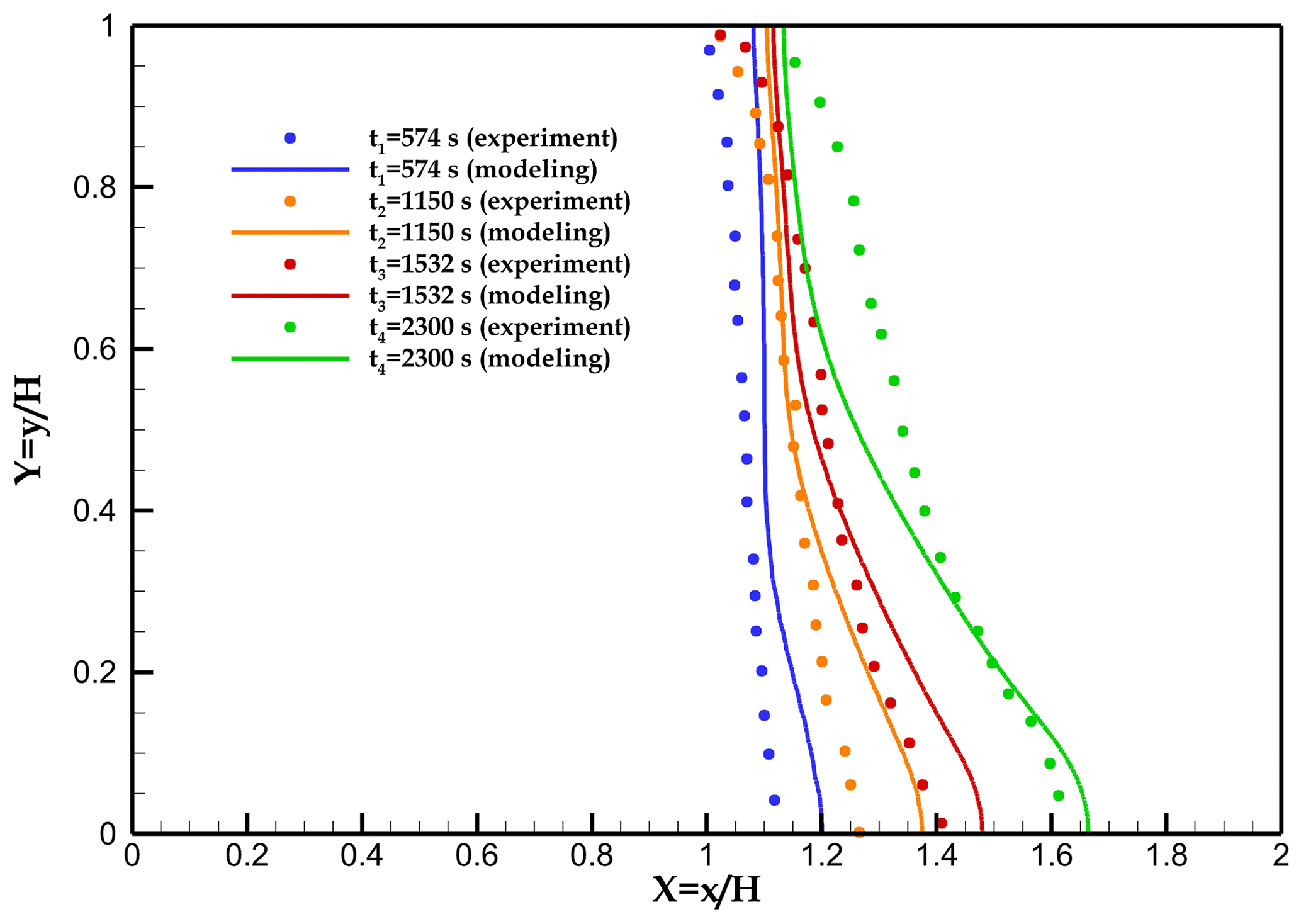
Figure 5 Evolution of the modelled ice–water interface during melting in comparison with experimental data by Virag et al. (2006).

4 Results

4.1 Stagnant liquid water (SLW) versus free convection (FC)

The effect of free convection in the heterogeneous, ice-filled karst environment (see Fig. 1) where the medium is surrounded by rock and prone to atmospheric warming from the top surface was conceptualised in Sect. 2. Here, we investigate the effect of free convection in more detail, considering two scenarios under identical thermal settings: (1) stagnant liquid water (SLW) and (2) free convection in liquid water (FC). Figure 6 illustrates the ice volume fraction (1−θ) for different time steps at 3, 6, and 9 h for these two scenarios and for an aperture size A_p=10 cm (see Fig. 1b for a description of the computational domain geometry). For each specified time step, the SLW results are shown on the left and the FC results on the right. The difference between these two scenarios in terms of melting rate is obvious. When convection is disregarded (SLW), the melting front is nearly horizontal except close to the walls, where a steep slope is observed. The higher thermal diffusivity of the rock (${\mathit{\alpha }}_{\mathrm{r}}=\frac{k_{\mathrm{r}}}{{\mathit{\rho }}_{\mathrm{r}}{c}_{p,\mathrm{r}}}=\mathrm{8.8}\times {\mathrm{10}}^{-\mathrm{7}}$ m² s⁻¹) compared to that of the liquid water (${\mathit{\alpha }}_{\mathrm{l}}=\frac{k_{\mathrm{l}}}{{\mathit{\rho }}_{\mathrm{l}}{c}_{p,\mathrm{l}}}=\mathrm{1.3}\times {\mathrm{10}}^{-\mathrm{7}}$ m² s⁻¹) results in faster heat propagation in the rock and enhanced melting of the ice closer to the rock. When free convection is considered (FC), the advection of heat by the flow results in faster propagation of the melting front, with an inversion of its curvature (the meting front propagates faster in the centre of the cleft than close to the walls).

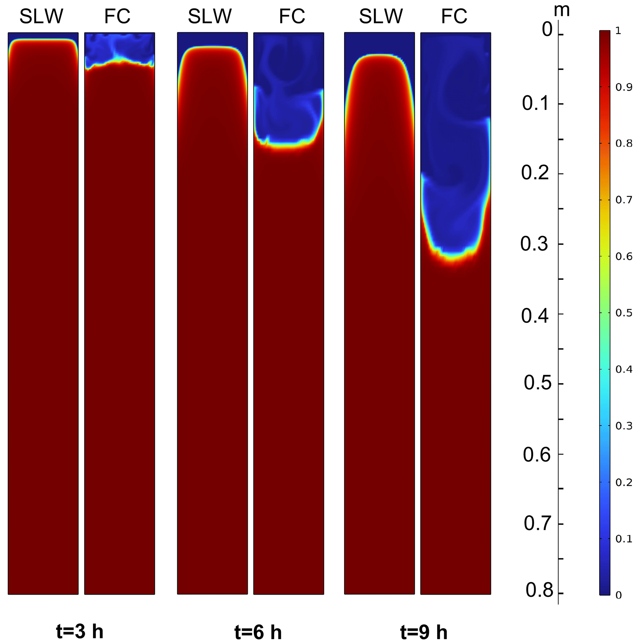
Figure 6 Contour of the ice volume fraction (1−θ) for stagnant liquid water (SLW) and free convection (FC). A_p=10 cm, H_dom=0.8 m, and W=1 m.

Figure 7 displays the melting rate for both previous scenarios, SLW and FC. Because the initial temperature was −1 °C, the melting starts with ca. 1 h delay in both cases. Then the melting rate and the meltwater depth increase with time in response to the temperature increase at the top surface. After 9 h, the melting rate is nearly an order of magnitude larger for FC (5.1 kg s⁻¹) than for SLW (0.6 kg s⁻¹). An animation file showing the evolution of the ice fraction can be found in the “Video supplement” section of the paper (Sedaghatkish and Luetscher, 2023).

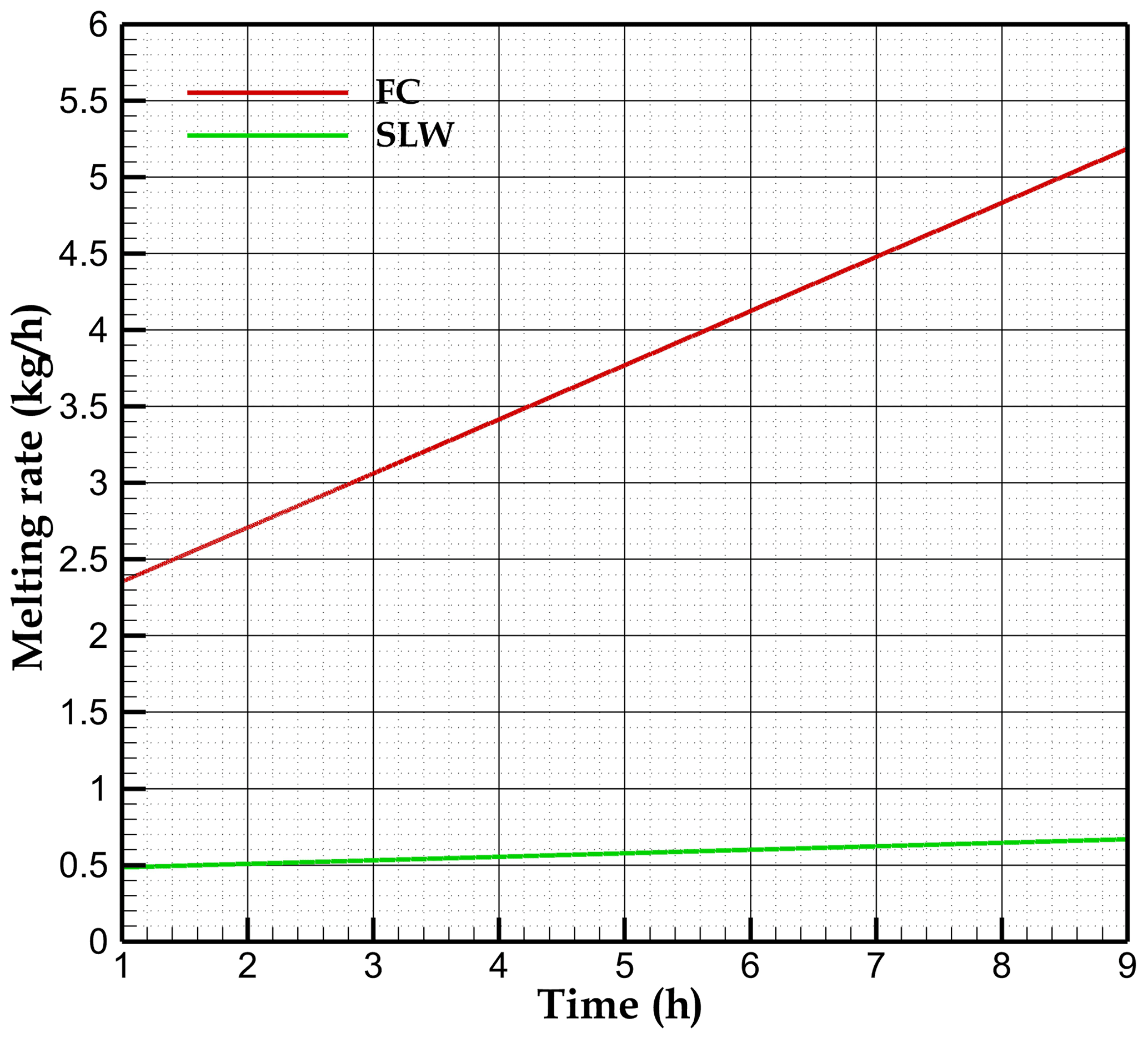
Figure 7 The melting rate versus time considering stagnant liquid water (SLW) and free convection (FC).

Figure 8 displays the temperature field of ice, water, and the surrounding rock after 9 h. In the FC case, most of the melted part of the cleft is in the temperature range from 0 to 1 °C, with a high temperature gradient localised in a thin layer close to the ground surface (Fig. 8b). In contrast, the temperature field in the SLW case varies more evenly from the ground surface to the melting front (Fig. 8a). This confirms that the circulation of water inside the cleft results in a thermal bridge between the ice interface and the top atmosphere. The extent of the mixing zone induced by FC can be much higher than the diffusion length in the case of SLW.

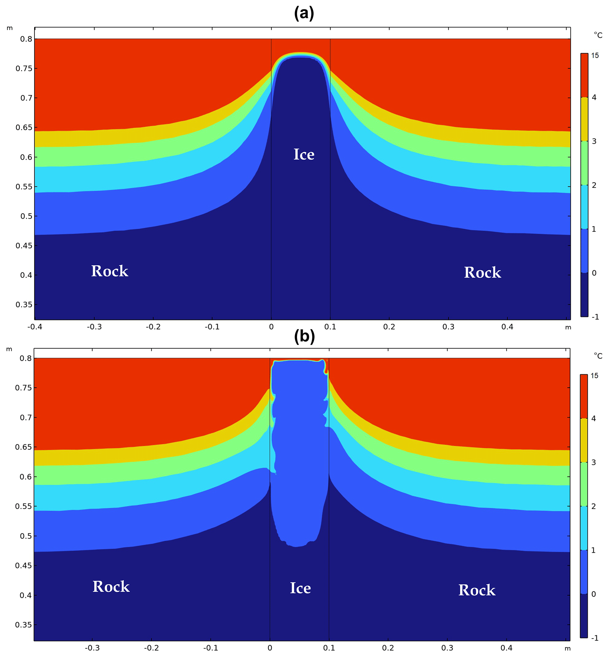
Figure 8 The temperature contour at t=9 h for (a) stagnant liquid water (SLW) and (b) free convection (FC).

Figure 9 displays the left-wall temperature as function of depth at different times for both scenarios. Although the melting rate for FC at t=3 h is much higher than for SLW at the same time, their corresponding wall temperatures are close to each other. At longer time steps, the distinction between scenarios becomes more pronounced due to the increasing intensity of free convection.

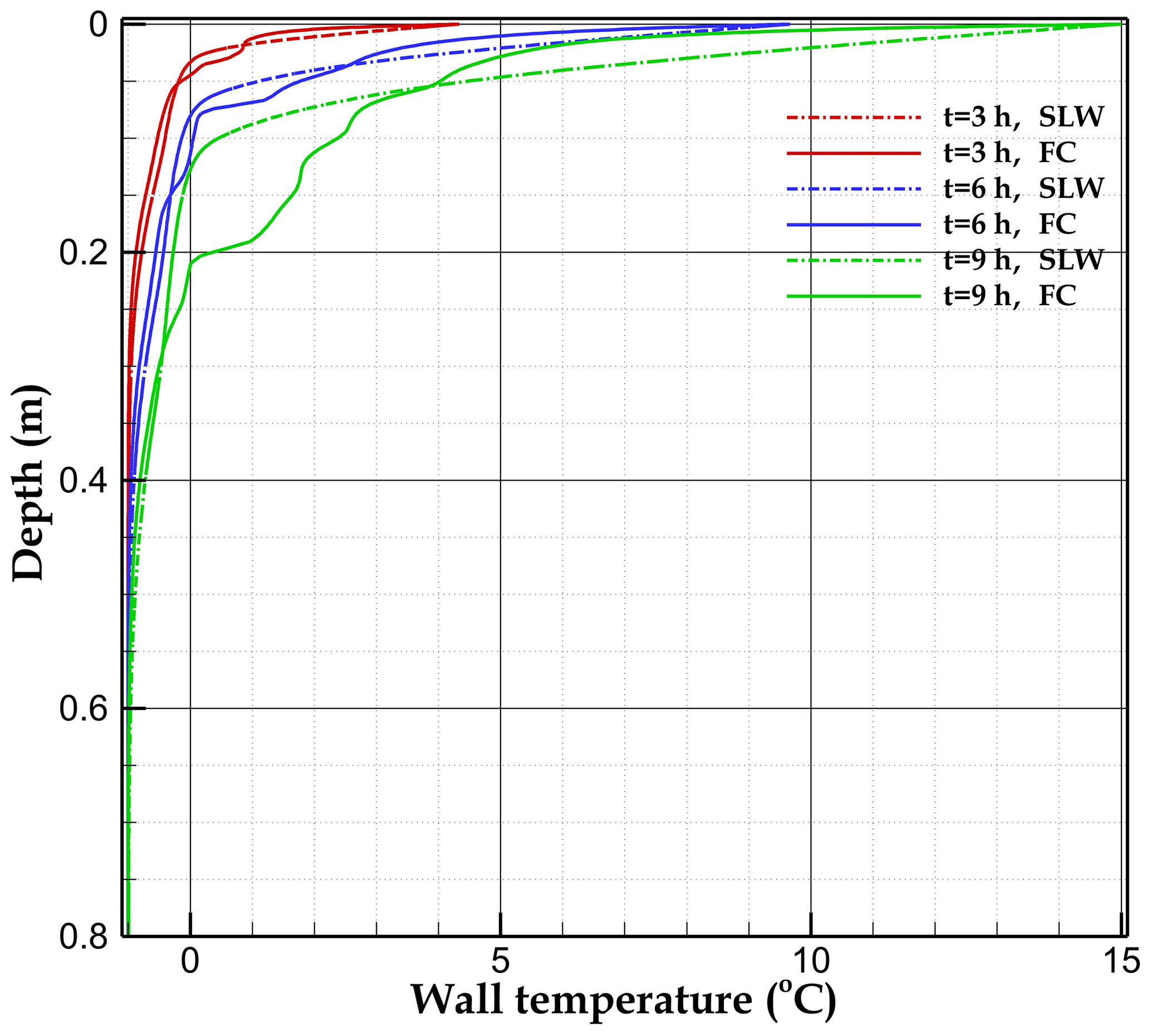
Figure 9 Left wall (rock–water interface) temperature as a function of depth for stagnant liquid water (SLW) and free convection (FC).

Figure 10 displays the velocity magnitude as well as the flow in the water domain at different times. Vanishingly small velocity is predicted by the model wherever the water fraction is zero. Liquid water circulation generates a range of local velocities, mixing the water and homogenising the water temperature. As the melting of ice advances and the meltwater amount increases, the velocity of water within the mixing zone increases, thereby accentuating the significance of free-convective flux.

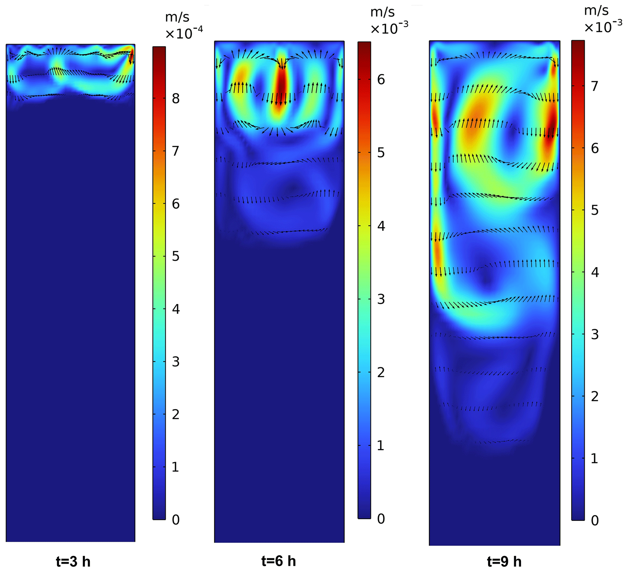
Figure 10 Velocity magnitude field in the upper 40 cm of the ice cleft at different times. Zero velocity shows solid ice.

4.2 The effect of aperture size on melting rates

The cleft aperture determines the size of the domain and controls the initial ice mass. We considered aperture sizes of 2, 10, 20, and 50 cm in the parametric study. In order to remove the effect of cross-sectional area associated with different aperture sizes, we refer to the melting rate per unit of cross-sectional area ($\mathrm{kg}{\mathrm{h}}^{-\mathrm{1}}{\mathrm{m}}^{-\mathrm{2}}$).

Figure 11 illustrates the effect of the aperture size on the melting rate as a function of time. For the SLW case, heat transfer is mainly driven by diffusion into the rock, which has a greater diffusivity than water (see the temperature contour in Fig. 8a). At a given depth, the rock is warmer than the water. The ice directly in contact with the rock thus melts faster. This explains the larger specific melting rate obtained with the smallest aperture (A_p=2 cm). In the presence of free convection, the melting rate after 9 h is almost the same for aperture sizes of 2 and 10 cm (50 $\mathrm{kg}{\mathrm{h}}^{-\mathrm{1}}{\mathrm{m}}^{-\mathrm{2}}$). For greater aperture sizes, the effect of free convection becomes more significant, resulting in the increase in the melting rate, which reaches about 110 $\mathrm{kg}{\mathrm{h}}^{-\mathrm{1}}{\mathrm{m}}^{-\mathrm{2}}$ for the 50 cm aperture size. Figure 11 shows that the melting rate considering free convection with a 2 cm aperture-size (50 $\mathrm{kg}{\mathrm{h}}^{-\mathrm{1}}{\mathrm{m}}^{-\mathrm{2}}$) is about twice the rate of the pure-conduction case. For higher aperture sizes, the difference in melting rates reaches about an order of magnitude.

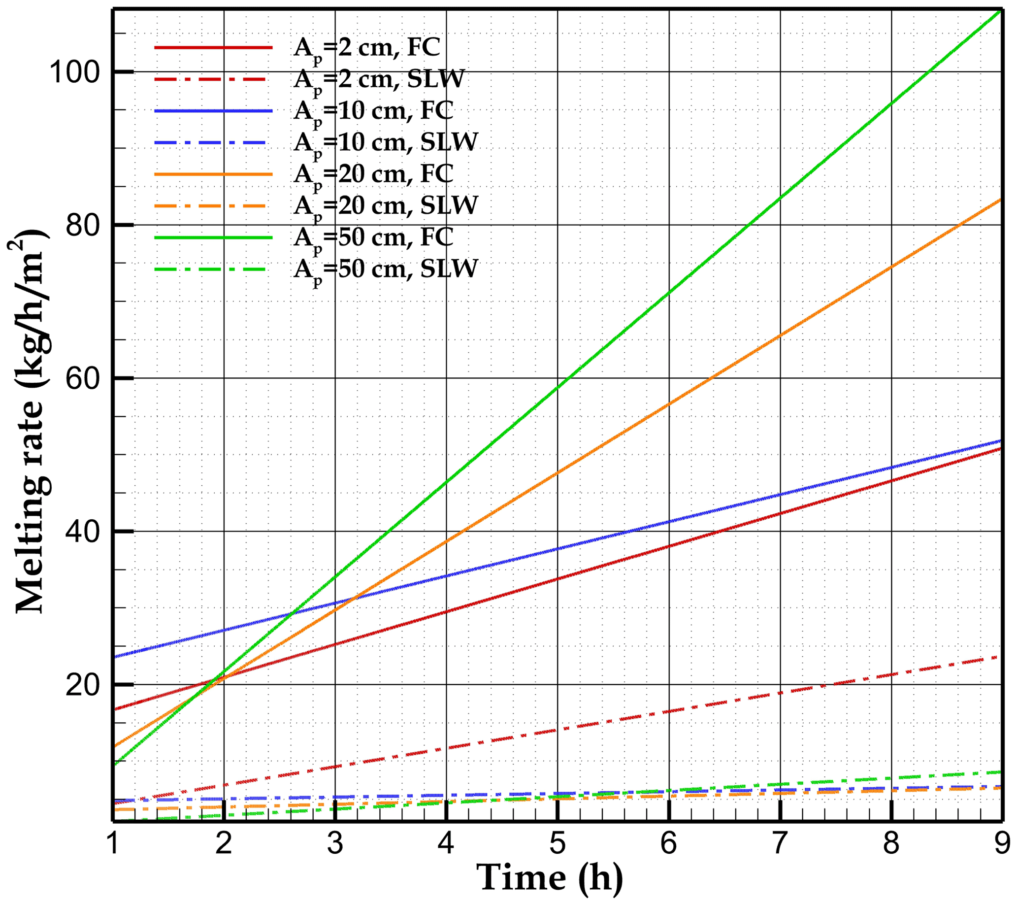
Figure 11 Effect of the aperture size on the melting rate for stagnant liquid water (SLW) and free convection (FC).

In the present work, we simulated 9 h of atmospheric temperature increase. When the aperture size A_p was varied from 2 to 50 cm, the liquid height H at the end of the simulation ranged from approximately 30 to 40 cm, and the convection cell occupied the entire liquid domain. However, the liquid height reached after 9 h is only a small part of the actual height of the cleft (commonly up to 10 m). H is expected to increase if longer times are considered. The question arises whether the free-convection cells always fill the entire liquid domain at longer timescales, despite the increase in friction due to the lower aspect ratio $A_p/H$. If the convection cell occupies only a part of the cavity, the efficiency of heat transfer between the ground surface and the melting front will be reduced. The significance of free convection can be assessed from the value of the dimensionless Rayleigh number

$$\begin{array}{}\text{(15)}& \mathit{Ra}={\displaystyle \frac{g\mathit{\beta }\left(T_{\mathrm{c}}-T_{\mathrm{H}}\right)H^{\mathrm{3}}}{{\mathit{\alpha }}_{\mathrm{l}}{\mathit{\nu }}_{\mathrm{l}}}},\end{array}$$

where (T_c−T_H) is the temperature difference between bottom and top surfaces and ${\mathit{\alpha }}_{\mathrm{l}}=k_{\mathrm{l}}/\left({\mathit{\rho }}_{\mathrm{l}}{c}_{\text{pl}}\right)$ and ${\mathit{\nu }}_{\mathrm{l}}={\mathit{\mu }}_{\mathrm{l}}/{\mathit{\rho }}_{\mathrm{l}}$ are the liquid water diffusivity and kinematic viscosity, respectively. Ra represents the ratio of the diffusion time over the free-convection time (Ra∼10⁸ in the numerical experiments presented in this article). In a cavity with infinite lateral dimensions (i.e. for $A_p/H\to \mathrm{\infty }$), free convection is triggered for Ra≳10³ (otherwise the conductive state is stable; see Bergman and Lavine, 2017, for more information about the Rayleigh–Bénard instability). However, in the confined geometry considered in this work, the presence of the vertical walls must be considered. Rohsenow et al. (1998) provide the following condition for convection onset, which takes into account the stabilising effect of the vertical walls for A_p≪H in the limiting case of perfectly conducting walls:

$$\begin{array}{}\text{(16)}& \mathit{Ra}\gtrsim {\mathrm{10}}^{\mathrm{2}}\times {\left({\displaystyle \frac{H}{A_p}}\right)}^{\mathrm{4}}.\end{array}$$

Inserting Eq. (15) into Eq. (16) yields the maximum value of the liquid height H, for which the free-convection cell extends from the ground surface to the melting front:

$$\begin{array}{}\text{(17)}& H\lesssim {\mathrm{10}}^{-\mathrm{2}}\times {\displaystyle \frac{g\mathit{\beta }(T_{\mathrm{c}}-T_{\mathrm{H}})A_p^{\mathrm{4}}}{{\mathit{\alpha }}_{\mathrm{l}}{\mathit{\nu }}_{\mathrm{l}}}}.\end{array}$$

Considering that the liquid region at temperature T>4 °C is stable and that the isotherm 4 °C is close to the top of the cleft when the free-convection cell fills the entire cavity (see Fig. 8b), we obtain $(T_{\mathrm{c}}-T_{\mathrm{H}})=-\mathrm{4}$ °C. Using the physical properties from Sect. 2.3 and A_p=2 cm (the minimum aperture size considered in this study) yields H≲10 m, which is also the order of magnitude of the maximum cleft height. Therefore, free-convection cells should always extend throughout the melted region for A_p≳2 cm. Note that the assumption of perfectly conducting walls used in Eq. (16) is less favourable to convection than finite conductivity (Rohsenow et al., 1998). Equation (17) is thus expected to underestimate the higher bound of H corresponding to fully developed free-convection cells.

4.3 Application to field observations

The model is applied to a case study from the Monlesi ice cave, Switzerland (Luetscher et al., 2008). The main purpose is to qualitatively compare the field data with the model output and test how the pure-conduction model can treat these problems.

The Monlesi ice cave is a low-elevation sporadic mountain permafrost site controlled by a peculiar ventilation regime associated with multiple cave entrances located at a similar elevation (Luetscher et al., 2008). The ca. 600 m² cave chamber is partly filled with perennial congelation ice fed by a number of vertical clefts with width ranging from 10¹ to 10³ mm. Seasonal freezing seals them periodically, hindering any further water drainage from the epikarst (Fig. 12a). The vertical distance between the external ground surface and the cave ceiling reaches ca. 20 m. Seasonal and daily outside temperature fluctuations thaw the ice and freeze the meltwater in these rock clefts.

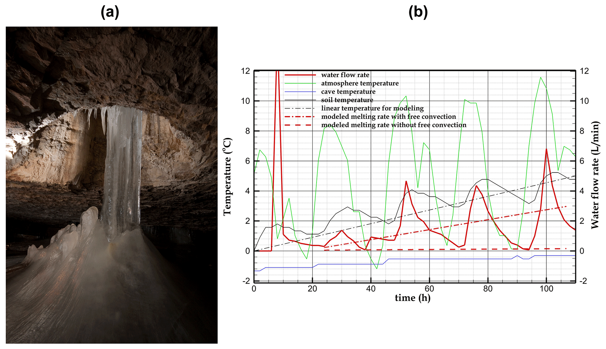
Figure 12 (a) Ice-filled cleft in the Monlesi ice cave. (b) Field data including atmosphere (green), soil temperature (black), and cave temperature (blue), as well as the water flow rate measured at the fissure outlet (red) in the Monlesi ice cave. The modelled melting rate considering free convection (dashed–dotted red line) is compared to a case including only heat conduction (dashed red lines).

The main cleft (subcutaneous flow) was instrumented to measure discharge rates at 30 min intervals using a pressure probe set at the bottom of a 1 m long perforated PVC tube capturing the inlet. The water height measured in the tube is converted to discharge (Q, in L min⁻¹), with an empirically calibrated rating curve checked by nine manual bucket gauges between 0 and 13 L min⁻¹ with an uncertainty of ±10 % (Luetscher et al., 2008).

Cave air temperatures were measured using negative temperature coefficient thermistors with a resistance of ca. 29.5 kOhm at 0 °C and a temperature coefficient of about 5 % °C⁻¹ (YSI 44006). The thermistors were calibrated in a bath of melting ice to an accuracy of ±0.1 °C. The thermistors were spaced at 2 m intervals in two chains comprising 19 sensors that were dispatched in the main cave chamber (Luetscher et al., 2008). Air temperatures were recorded at 1 h intervals and logged externally on a Campbell CR10X data logger with two multiplexer logging units.

Figure 12b displays the atmosphere and soil temperatures at a 10 cm depth during 4.5 d (from 13 to 17 April). No rainfall is recorded during this time period, and the surface is free of snow. The soil temperature increases with a regular trend between 0 and 5 °C and is noticeably attenuated compared to atmospheric temperature fluctuations. The cave temperature is almost constant around −1 °C, implying that there is no melting from the bottom of the ice cleft. The atmospheric daily temperature variation induces a water flow rate (0–12 L min⁻¹) with a trend similar to the surface temperature, supporting an origin associated with the melting process of ice-filled clefts surrounding the cave.

To assess the melting rate, we considered the same conceptual model as in Fig. 1. A linear temperature rise from 0 to 5 °C during 4.5 d was assumed at the top boundary (dashed–dotted black line in Fig. 12b). This temperature rise is similar to the temperature evolution measured in the soil (solid black line in Fig. 12b). In contrast to our model, meltwater drains deeper into the subsurface. The uncertainty about the cleft geometry is, however, very high, and we do not know how many fissures feed this water inlet. While our conceptual model is based on a closed cavity for the ease of simulation, the ice-filled cleft could be connected to a network of partially saturated smaller clefts (as in the epikarst) that drain the meltwater into the main vertical inlet at the top wall of the Monlesi ice cave. Eventually, our simplified 2D geometry only approaches the real 3D environment since other convection cells emerge along the cavity width that cannot be modelled in 2D.

A rough estimate of the cavity geometry (computational domain) assumes an initial ice-filled cleft with a depth of 3 m (H_dom=3 m), a 10 cm aperture size (A_p=10 cm), and a typical length on the order of 1 m. The modelled melting rate is on the same order of magnitude as the water flow rate measured in the cave (dashed–dotted red line in Fig. 12b). A purely conduction based model underestimates the melting rate by >1 order of magnitude as compared to the case considering free convection (dashed in Fig. 12b).

5 Discussion

In this study, we assumed a constant aperture size for modelling ice melt at the daily timescale, but it should be noted that in the long-term, the repeated freeze–thaw cycles can deteriorate the host rock clefts due to propagation and coalescence of older ones. Maji and Murton (2021) investigated the mechanism and transition of micro-cracking and macro-cracking during freezing and thawing and developed a statistical modelling of crack propagation dynamics based on tension and shearing.

Our results show that under similar thermal configurations, conduction may not be the principal heat flux, and permafrost degradation in heterogeneous and ice-rich media may be much faster than anticipated. This is particularly relevant at high elevations where a clear relationship is observed between rockfall activity and permafrost thawing (Gruber et al., 2004; Ravanel and Deline, 2011; Savi et al., 2021; Morino et al., 2021). In karst systems and fractured aquifers where secondary porosity is exceptionally well developed, frozen conduits or fractures may all of a sudden drain water into the depths and change the local hydrological regime, leading a thermal anomaly within the surrounding permafrost (Phillips et al., 2016). The subsequent freeze–thaw processes may lead to the precipitation of so-called cryogenic cave calcites (Žák et al., 2018), a secondary mineral precipitate increasingly used as a proxy for paleo-permafrost conditions (Spötl et al., 2021; Töchterle et al., 2023). In contrast to purely conductive systems, our results support a model where rapid hydrological recharge, e.g. due to extreme rainfall events, may accelerate the thawing of mountain permafrost (Luetscher et al., 2013) and thus questions classical interpretations of the formation of cryogenic calcites. But also at shallower depth, acknowledging the potential role of convective heat fluxes in ice-rich permafrost degradation may help predict the rate of greenhouse gas release, mainly carbon dioxide and methane, due to the decomposition of formerly frozen organic matter (Schaefer et al., 2014; Schuur et al., 2015). The intensity of free convection in soil depends strongly on the Rayleigh number, which in turns depends on the permeability and dimensions of the soil layer, making it negligible, e.g. Kane et al. (2001), or significant, e.g. Jazi et al. (2024), with respect to the total heat transfer.

Pure water with a melting point at 0 °C was considered in the present study. However, limestone dissolution results in the mineralisation of the meltwater. The consequences are twofold: (1) the melting point is shifted to lower temperatures (in the range of −4 to 0 °C; see Tubini et al.; 2021, McKenzie et al., 2007; and Rühaak et al., 2015) and (2) the variation in density with salt concentration could impact buoyancy, resulting in different flow patterns (thermo–solutal convection; see, for instance, Mergui et al., 2002). The significance of the liquid-phase composition could be assessed by numerical simulations and should be considered in future work.

We did not consider any drainage of air or water inside the cleft or in its immediate vicinity. Forced convection induced by drainage could also contribute to the formation of a thermal bridge between the ground surface and the melting front, as suggested by Hasler et al. (2011). More work coupling field observations with numerical simulations including forced and free convection will be necessary to assess their relative significance and to determine the conditions under which one or the other effect dominates heat transfer.

6 Conclusion

A quantification of the melting rate of ice-rich permafrost in heterogeneous media is essential to assess the speed of permafrost degradation. Our model relies on a 2D approach coupling free convection (buoyancy-driven flow) in a vertical cleft with conduction in the surrounding homogeneous rock. Increasing the temperature of the ground surface can generate free-convection cells because water density increases between 0 and 4 °C (a property specific to water). The convection cells generate a thermal bridge between the atmosphere and the melting front, resulting in the formation of a mixing zone with quasi-uniform temperature in the water column. This dramatically enhances the melting rate of interstitial ice when compared to models assuming stagnant liquid water (about an order of magnitude after 9 h for an aperture size of 10 cm). In contrast to scenarios assuming conduction in stagnant liquid water, for which the temperature signal from the atmosphere is fully attenuated beyond a certain distance known as the diffusion length, the presence of free convection extends over greater distances. This thermal penetration also exerts an influence on the surrounding rock. Despite simplifying assumptions in the model and many uncertainties about the cleft geometry and the measured water flow rate, the melting rate predicted by the model including free convection fits the order of magnitude measured in the Monlesi ice cave (Fig. 12).

The significance of free convection should also be estimated in similar thermal configurations with different geometries, such as cylindrical conduits or 3D cavities. Furthermore, the effect of free convection is not limited to hourly or daily oscillations and can be studied over much longer timescales, including centennial to millennial fluctuations. Currently, the computational costs are the main barriers to including free convection in long-term simulations. Full coupling of the momentum and energy equations requires the time steps to be much smaller compared to simple conduction-based models. Further investigations are thus ongoing to reformulate the governing equations and simplify them for simulations over longer timescales. Moreover, refreezing processes that fully represent the long-term evolution of such a system have yet to be considered.

Eventually, the effect of water free convection on the ice melting rate is not limited to permafrost regions. For instance, the melting of icebergs can also be impacted by water free convection (Couston et al., 2021; Hester et al., 2021), increasing production of freshwater in oceans with potential impacts on the climate at the global scale.

Appendix A: Sensitivity of the model to the melting temperature range ΔT

The sensitivity of the melting rate to the melting temperature range ΔT is displayed in Fig. A1. Similar results are obtained for $\mathrm{\Delta }T\le \pm \mathrm{0.7}$ °C. $\mathrm{\Delta }T\le \pm \mathrm{0.5}$ °C was thus selected in all simulations as a value giving a good approximation of the pure-water melting rate.

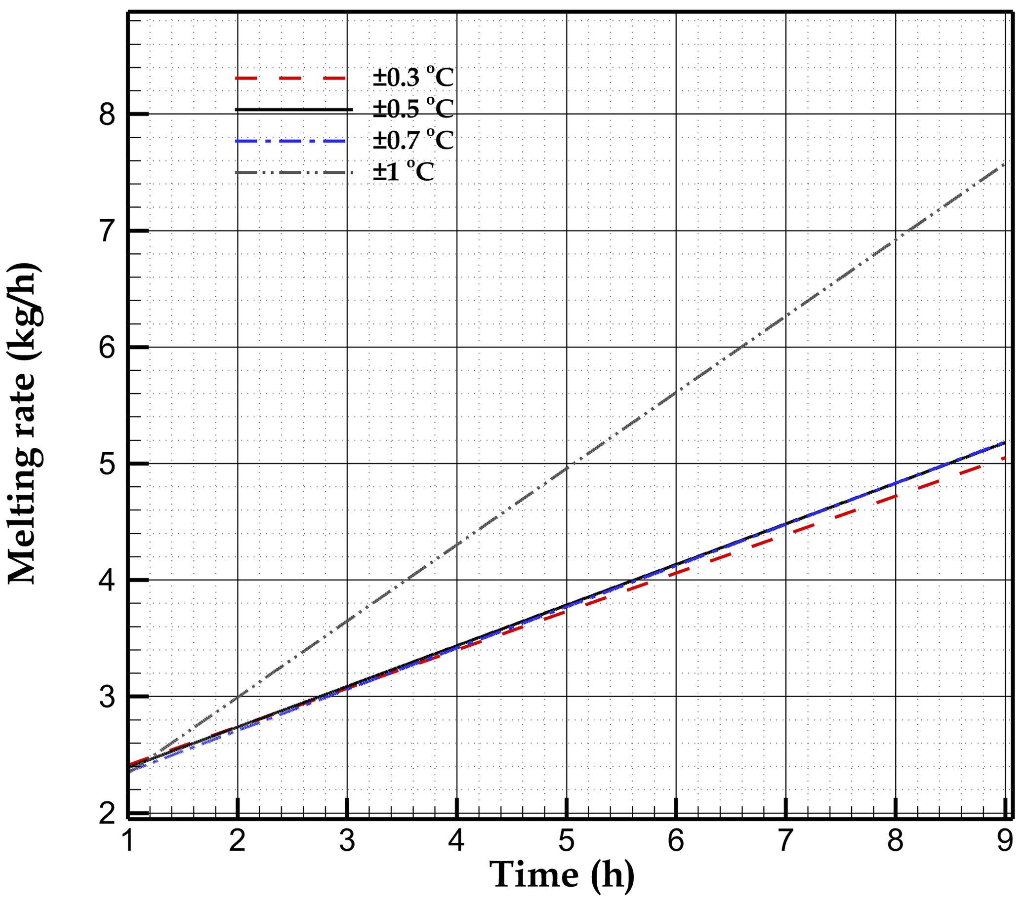
Figure A1 Effect of the melting temperature range ΔT on the melting rate predicted by the model (FC case, A_p=10 cm, H_dom=0.8 m, W_dom=1 m).