Quantifying the influence of snow over sea ice morphology on L-band passive microwave satellite observations in the Southern Ocean

Antarctic snow on sea ice can contain slush, snow ice, and stratified layers, complicating satellite retrieval processes for snow depth, ice thickness, and sea ice concentration. The presence of moist and brine-wetted snow alters microwave snow emissions and modifies the energy and mass balance of sea ice. This study assesses the impact of brine-wetted snow and slush layers on L-band surface brightness temperatures (TBs) by synergizing a snow stratigraphy model (SNOWPACK) driven by atmospheric reanalysis data and the RAdiative transfer model Developed for Ice and Snow in the L-band (RADIS-L) v1.0 The updated RADIS-L v1.1 further introduces parameterizations for brine-wetted snow and slush layers over Antarctic sea ice. Our findings highlight the importance of including both brine-wetted snow and slush layers in order to accurately simulate L-band brightness temperatures, laying the groundwork for improved satellite retrievals of snow depth and ice thickness using satellite sensors such as Soil Moisture and Ocean Salinity (SMOS) and Soil Moisture Active Passive (SMAP). However, biases in modelled and observed L-band brightness temperatures persist, which we attribute to small-scale sea ice heterogeneity and snow stratigraphy. Given the scarcity of comprehensive in situ snow and ice data in the Southern Ocean, ramping up observational initiatives is imperative to not only provide satellite validation datasets but also improve process-level understanding that can scale up to improving the precision of satellite snow and ice thickness retrievals.

1 Introduction

Snow on sea ice significantly influences the polar climate and ecosystems by mediating mass and energy exchanges during air–sea interactions, as well as key biological and biogeochemical processes (Sturm and Massom, 2017). Recent record lows in the Antarctic sea ice extent, with departures from the 1981–2010 long-term average in excess of 7 standard deviations, underscore the urgency to understand the drivers of Antarctic sea ice variability. To better quantify the drivers, there is a need to improve our observational capacity of key sea ice variables, including its overlying snow cover, a key variable for the reliable estimation of ice thickness and volume (Laxon et al., 2013; Kaleschke et al., 2016). Yet, our knowledge regarding the characteristics of snow over Antarctic sea ice remains limited, partly due to the Southern Ocean's remote and harsh environment and the complexities of the snowpacks found there.

In the Antarctic, the weight of accumulating snow can push the ice surface beneath sea level (Nicolaus et al., 2009; Sturm and Massom, 2017). This usually entails flooding, which can lead to negative freeboards, slush formation (Jutras et al., 2016; Webster et al., 2018) that freezes to snow ice (Merkouriadi et al., 2017; Zhaka et al., 2023). During winter, the permeation of seawater into the snowpack becomes extensive, either infiltrating laterally at ice floe edges or seeping through fractures in less consolidated ice (Maksym and Jeffries, 2000). This flooding is preconditioned by high ocean heat flux melting ice from the bottom and/or snow redistribution and precipitation on top, which can lower the snow–ice interface below sea level (Lytle and Ackley, 2001; Ackley et al., 2020).

Such conditions allow seawater's brine to infiltrate the snow, resulting in a layer of slush or snow ice, which constitutes up to one-third of the total sea ice mass in the Antarctic region (Maksym and Markus, 2008; Vancoppenolle et al., 2009). This layer will form shortly after flooding due to its “self-balancing” mechanism (Sturm and Benson, 1997) and will reassert the hydrostatic balance and increase the sea ice freeboard. Complex processes occur at the snow–ice interface, such as the further intrusion of seawater into the snowpack, as well as the gradual drainage of brine within the newly formed snow ice. Notably, even when seawater flooding is not present (Massom et al., 1998; Toyota et al., 2011), snowpacks may still house saline and damp layers at their base. Through capillary suction, the brine in sea ice can ascend into the basal snow layer (Massom et al., 2001; Lewis et al., 2011), resulting in brine-wetted snow. This phenomenon can be observed when snow is deposited on the surface of new sea ice (Takizawa, 1985; Deming et al., 2010) or when sporadic warming events amplify the ice's porosity and permeability, enabling upward brine movement (Tucker et al., 1992). In addition to brine-wetted snow, other factors during winter, such as the atmospheric forcings, including precipitation variability, strong winds, and repeated melt–refreeze cycles, contribute to the snow's complex stratigraphy (Sturm and Massom, 2017). These factors result in brine drainage in the slushy layer (Maksym and Jeffries, 2000), variations in snow grain size and density, meltwater percolation and refreezing within/under the snow cover, and the formation of ice lenses (Ji et al., 2021; King et al., 2020b). Such complexities not only influence the snow's thermodynamic properties and surface albedo but also recalibrate the energy fluxes, subsequently altering the sea ice's mass balance (Massonnet et al., 2019). Concurrently, these stratified layers induce shifts in the snow's dielectric characteristics, thereby affecting its microwave emissivity and the retrieval of various sea ice parameters (Fuller et al., 2021).

Microwave emission from the snow-covered sea ice is determined not only by its bulk properties, such as grain size, density, liquid water content, and salinity, but also by the intricacies of its stratigraphy and the characteristics of each layer. Specifically, layers of wet or saline snow are particularly absorbent of microwave emissions (Picard and Fily, 2006; Geldsetzer et al., 2009). Even in dry snow, variations in grain size and density can significantly alter microwave emission (Tsang et al., 2000). For flooded snowpacks, the emergence of slush at the snow–ice interface or wet snow atop this slush layer can inhibit emissions from the ice beneath the snow's base (Ulaby et al., 2014). Our primary challenge is to deepen our understanding of how these physical snow attributes influence microwave emissions. Such insights are pivotal for enhancing our capacity to accurately monitor sea ice concentration (Willmes et al., 2014), thickness (Willatt et al., 2010; Giles et al., 2008; Nandan et al., 2017, 2020), type (Melsheimer et al., 2023), snow depth (Rösel et al., 2021), sea ice drift (Lavergne and Down, 2023), and melt onset timings (Arndt et al., 2016). With the evolving climate conditions in Antarctica, it is anticipated that snow melting and refreezing processes will become more prevalent, necessitating refined satellite retrieval algorithms for sea ice and snow properties (Raphael and Handcock, 2022; Wever et al., 2020).

Typically, snow over sea ice comprises numerous layers with different physical characteristics rather than a uniform slab (Massom et al., 2001; Sturm et al., 1998), e.g. new snow, hard slab, faceted snow, depth hoar, and saline slush (Massom et al., 1998; Sturm and Benson, 1997). Established radiative transfer models, such as MEMLS (Tonboe et al., 2006), DMRT-ML (Schmidt and Wauer, 1999), and SMRT (Picard et al., 2018), despite their contributions, have been limited in representing the true complexity of snow stratigraphy over sea ice, mainly tailoring to single-layer simulations adapted to dry, cold conditions (Rostosky et al., 2018; Kilic et al., 2019). Addressing this gap, our study endeavours to enhance the understanding of snow stratigraphy's impact on passive microwave emission, leveraging more sophisticated radiation transfer models to simulate the effects of two snow layers – fresh snow overlaying a brine-wetted layer – on brightness temperatures (TBs) over the Southern Ocean. This study, grounded in a meticulous analysis using the enhanced RAdiative transfer model Developed for Ice and Snow in the L-band (RADIS-L; Zhou et al., 2017), aims to foster a refined understanding of the snow stratigraphy's impact on passive microwave emission while paving the way for sophisticated satellite retrievals through nuanced radiation transfer models. The paper is structured as follows: Sect. 2 describes the observations and satellite datasets utilized in the study. Following this, the approach adopted in the incorporation of a new parameterization representing brine-wetted and slush snow in RADIS-L v1.1, alongside the snow stratigraphy model (SNOWPACK) analysis, is introduced in Sect. 3. The subsequent sections, Sects. 4 and 5, contain critical examinations of the observed snow properties with regard to the simulated TBs against L-band satellite measurements, offering insights into model discrepancies and the outcomes of sensitivity studies. Finally, the conclusion (Sect. 6) rounds off the discussion with a contemplative reflection on the study's contributions and future research trajectories.

Figure 1 (a) Map of Antarctica illustrating the geospatial distribution of various in situ and airborne observation data: Operation IceBridge (OIB) (purple circles), AWI purchases (yellow stars), IMB (orange crosses), ASPeCt (blue squares), all PS81 ice stations (green triangles), snow observations collected during several Polarstern cruises (pink triangles), ZS and DS stations (red rhombi), and SIPEX II (olive-green triangles). (b) A zoomed-in view of the Weddell Sea, showcasing detailed data points. (c) Schematic representation illustrating the functioning of RADIS-L v1.1 in a three-layer system: dry snow, brine-wetted snow, and sea ice.

2 Data

2.1 In situ measurements

2.1.1 ASPeCt ship-based measurements

Information on the concentration, thickness, and snow cover characteristics of Antarctic sea ice has been collected from ship cruises as part of the Antarctic Sea Ice Processes and Climate (ASPeCt) programme (Worby et al., 1996; Worby and Ackley, 2000; Worby et al., 2008) (blue squares in Fig. 1) since the 1980s. In this paper, we used ASPeCt sea ice thickness, ice type, snow depth, and surface temperature observations available from the European Space Agency Climate Change Initiative (ESA-CCI) sea-ice essential climate variable (ECV) project, phase 2 (ESA-SICCI2). These data include collections from June 2002 through December 2019 (Kern, 2019). ASPeCt represents data along ship trajectories and includes visually and manually conducted measurements. The temporal resolution is typically hourly but can vary by cruise. Depending on conditions, a single ship-based observation of the sea ice generally represents an observation area with a semi-minor axis close to 1 km and a semi-major axis between an estimated 1 and 2.5 km.

2.1.2 Buoy measurements

Snow and ice mass balance buoys in the Weddell Sea

To supplement our study, we utilized data from autonomous ice-tethered platforms in the Weddell Sea collected in 2013 and 2014. Initially, we examined data from the Scottish Association for Marine Science (SAMS) ice mass balance buoys (IMBs) (Jackson et al., 2013), which are equipped with thermistor strings. Each string contains thermistors spaced every 2 cm, capable of measuring temperature and being heated. As reported by Wever et al. (2021a), the snow–ice interface is identified by the maximum of the first derivative in the vertical temperature profiles and diurnal variability in the profiles, and the accuracy in its location is estimated to be about 2–4 cm.

Additionally, we analysed data from snow buoys, which are equipped with four ultrasonic sensors approximately 1.5 m above the snow–sea ice interface at deployment: hourly snow accumulation is determined by averaging the four ultrasonic sensors. These buoys also measure air temperature and pressure. All data are recorded hourly and transmitted via an Iridium connection (Nicolaus et al., 2021).

IMB 2016T41 and the collocated snow buoy 2016S31 provide data over multiyear ice (MYI) starting in January 2016 (trajectories in Fig. 1). Here, we use data collected during the period from 30 April 2016 to 1 January 2017. Another two buoys, surveying the Weddell Sea during 2013 and 2014 and deployed as part of the Antarctic Winter Ecosystem and Climate Study (AWECS; ANT-XXIX/6) (Lemke, 2014), are used. They were installed on the ice station PS81/506 (PS81/517) and drifted with first-year ice (multiyear ice) floes (Arndt and Paul, 2018). These datasets (Wever et al., 2021a) were accompanied by 2 m height weather station data from an automatic weather station (AWS) buoy, providing snow depth, air temperature, humidity, and downwelling shortwave radiation. According to Wever et al. (2021a), IMB snow depths are less reliable than those from the sonic ranger on the AWS. Thus, for the PS81/506 and PS81/517 ice stations and buoys, we use sea ice thickness from the IMB and rely on the AWS for snow depth and air temperature.

Table 1 Summary of in situ and satellite data, including parameters used, period, and temporal resolution.

Ice mass balance buoys over Prydz Bay

In this study, we analysed snow depth and sea ice thickness on landfast ice in Prydz Bay from 2010 to 2018 using data from two ice mass balance (IMB) buoy types: the US Cold Regions Research and Engineering Laboratory (CRREL-IMB), identified by names starting with “ZS”, and the Snow and Ice Mass Balance Array (SIMBA), with buoy names starting with “DS”. Details of these buoys are included in Table 1. The CRREL-IMB buoys initially measure snow depth and ice thickness upon deployment. For continuous monitoring, they use an above-ice acoustic sounder to track the snow surface distance and an underwater sonar for ice bottom distance. The SIMBA buoys utilize a thermistor string to monitor changes in temperature profiles and detect heating-induced temperature differences, which assist in the determination of snow and ice thickness. The locations of these buoys and the corresponding sea ice parameters can be observed in Figs. 1 and B1.

2.1.3 Snow pit measurements from the Polarstern cruise

Snow density and salinity

To parameterize the emissivity and permittivity of the brine and wet-snow layers in the radiative transfer model, we rely on snow properties measured at the ice stations during PS81 (green triangles in Fig. 1) in ANT-XXIX/6 (Lemke, 2014). A total of 60 snow pits over first-year ice (FYI: PS81/506) and multiyear ice (MYI: PS81/517) were sampled from 13 stations between 21 June and 2 August 2013; FYI was sampled from 11 to 15 July 2013, and MYI was sampled from 29 July to 2 August 2013. Vertical snow density profiles, from the snow surface to the snow–sea ice interface, were determined using a 100 mL density cutter (Paul et al., 2017a). Vertical snow salinity profiles for each layer and each station were measured with a salinometer after melting the snow samples (Paul et al., 2017b). During PS81 (Paul et al., 2017a, b), density and salinity profiles were collected at 3 cm intervals. While salinity measurements were less frequent, they were always paired with density measurements at the same depth. We first analysed all collected data and then specifically examined paired density and salinity measurements to detail snow properties in each stratigraphy type.

Snow stratigraphy

Winter snow properties over sea ice in the Weddell Sea were based on data collected from 127 snow pits during several Polarstern cruises, including ANT-XXII/2 in 2004, ANT-XXIII/7 in 2006, PS81 ANT-XXIX/6 in 2013, and PS89 ANT-XXX/2 in 2014–2015 (represented by pink triangles in Fig. 1). Snowpack stratigraphy was characterized following Fierz et al. (2009) and was primarily based on visual observations. Snow type and size for each snow layer were assessed using an 8× magnifying glass and a millimetre-scale grid card, allowing for identification of the dominant grain size and type within each layer (Arndt and Paul, 2018). Layer hardness was also recorded.

2.1.4 Ice station measurements from the Sea Ice Physics and Ecosystems eXperiment II (SIPEX II) field campaign

Additional snow pit and drill hole measurements utilized in this study, obtained from five ice stations, were conducted in the seasonal sea ice zone off Wilkes Land, eastern Antarctica, between 23 September and 11 November 2012 (Toyota et al., 2016). Snow stratigraphy and vertical profiles of snow temperature, grain size, density, and salinity were collected at each snow pit from three locations along 100 m transects: 0, 50, and 100 m (Toyota et al., 2017; Heil et al., 2018). Furthermore, measurements of snow depth, sea ice thickness, and freeboard were obtained from drill holes along 11 transect lines, each 100 m in length, at 1 m intervals. Snow density and salinity were determined using a standard 3 cm high snow sampler with a volume of 100 cm³. A total of five transects were selected for the slush parameterization case study in Sect. 4.3, incorporating snow and ice measurements.

2.2 Operation IceBridge airborne measurements

To collect more snow and ice observations for the RADIS-L model validation, snow depth and sea ice thickness are compiled from the Operation IceBridge (OIB) airborne mission. The Airborne Topographic Mapper (ATM) and ultra-wideband snow radar flown on OIB provide several flight transects of snow and ice thickness. The conic scan of the ATM attains 1 m scale sampling of the sea ice topography nadir to the aeroplane, with a cross-track coverage of about 250 m at the nominal flight altitude of 460 m. The snow radar's effective footprint is 11 m across track and 14.5 m in the along-track direction (Kurtz et al., 2013).

Here, seven OIB flights over the Weddell Sea during October between 2010 and 2016 are used, including repeat surveys in 2011, 2014, and 2016 (purple lines in Fig. 1). Kurtz et al. (2015) provide snow depth and ice thickness from the 2010 flights, with the laser freeboard data interpolated to 40 m resolution centred within the snow radar footprints. With the highly accurate ATM-based elevation measurements, even at its raw footprint scale (Studinger et al., 2024), the uncertainty for the aggregated 40 m mean elevation and total freeboard is within a few centimetres. On the other hand, the uncertainty of the retrieved snow depth based on the OIB snow radar is shown to be dependent on the local averaging of waveforms and sea ice topographic features. The local averaging of waveforms before the retracking of snow and snow–ice interfaces significantly reduces the noise of the original snow radar waveforms. However, undersampling of thin snow distribution may lead to an overestimation bias due to the snow radar footprint (Kwok et al., 2017).

For the other four OIB flights, total freeboard is obtained from Kwok and Kacimi (2018), who follow the approach described by Kwok et al. (2012). Snow depths are obtained using the average from the wavelet (Newman et al., 2014) and peakiness algorithms (Jutila et al., 2021) available through the open-source pySnowRadar package developed by King et al. (2020a) via https://github.com/kingjml/pySnowRadar/tree/v1.1.1 (last access: 19 September 2024). Total freeboard is only calculated above the sea level reference in the presence of open water or leads within 10 km (Kwok and Kacimi, 2018). Derived snow depths from the above two sources are shown in Fig. B1. Figure B2 provides a summary of the in-situ-derived and OIB-derived snow depth and ice thickness observations.

2.3 Satellite TB measurements

2.3.1 SMOS

In November 2009 ESA launched the L-band (1.4 GHz) Soil Moisture and Ocean Salinity (SMOS) satellite to monitor the Earth's water cycle. This sensor measures the Earth's emitted radiation at 1.4 GHz at both horizontal and vertical polarization and at multiple incidence angles from 0 to 65° (Kerr et al., 2010). One data product used here consists of an average of the vertically and horizontally polarized TBs (L3B) (Kaleschke et al., 2012), gridded onto the NSIDC polar stereographic projection with a grid resolution of 12.5 km at 70° N/S, using the whole incidence angle range of 0–40°.

The other data product, the L3 globally polarized TB reprocessing RE07 product (Al Bitar et al., 2017), includes TBs from (1) all incidence angles and (2) all polarizations in the ascending and descending orbits projected on the global Equal-Area Scalable Earth Grid (EASE-Grid) 2.0 and can be freely downloaded from CATDS (available at ftp://ftp.ifremer.fr, last access: 19 September 2024).

2.3.2 SMAP

NASA launched the third Soil Moisture Active Passive (SMAP) sensor in January 2015, also dedicated to observing global soil moisture. SMAP carries both a radar (active) and a 1.4 GHz radiometer (passive). The radiometer is a conically scanning radiometer at a fixed incidence angle of 40° with an approximate spatial resolution of 36 km × 47 km (Piepmeier et al., 2017). Here, we use TBs from the SMAP radiometer twice-daily rSIR-enhanced version 2 (Brodzik et al., 2021) projected onto the EASE-Grid 2.0 at a resolution of 9 km. This dataset contains twice-daily enhanced-resolution brightness temperature data through the scatterometer image reconstruction (rSIR) algorithm.

2.4 Auxiliary data

2.4.1 AMSR-E/AMSR2

Sea ice concentration (SIC) is required as input for RADIS-L. The Advanced Microwave Scanning Radiometer for Earth Observing System (AMSR-E: 2002–2011) and AMSR2 (since 2012) provide daily estimates of SIC using various algorithms. In this study we use the SIC product based on the ASI sea ice algorithm (Spreen et al., 2008), which provides SIC at a spatial resolution of 6.25 km under the polar stereographic projection. NSIDC also has AMSR-E and AMSR2 SIC datasets based on the Markus and Cavalieri (2000) algorithm but at a coarser spatial resolution (12.5 km). However, the NSIDC product additionally includes 5 d running-mean-averaged snow depths (Markus and Cavalieri, 2000) and the daily-averaged TBs for each frequency and polarization. The snow algorithm depends on the gradient ratio of the vertically polarized TBs at 18.7 and 36.5 GHz and is only reliable over seasonal ice and in dry-snow conditions (Markus and Cavalieri, 1998). The snow depth and TB product from NSIDC, with a resolution of 12.5 km, are used to interpret surface variability in Sect. 5.1. The snow condition is flagged as snowmelt when the relative emissivity between 36.5 and 18.7 GHz decreases within 5 d.

2.4.2 ALOS PALSAR

In order to study the fine-scale sea ice features within the SMOS footprint, we use SAR images that cover the aforementioned in situ and airborne measurements in Sect. 5.1. Between 2006 and 2011, Phased Array type L-band (1.27 GHz) Synthetic Aperture Radar (PALSAR) data on board JAXA's Advanced Land Observing Satellite (ALOS) were acquired from different observation modes with adjustable polarization, resolution, swath width, and off-nadir angle. This study uses the newest ALOS PALSAR image data level 1.5 product from the wide-area observation mode (burst mode 1), or WB1, at the off-nadir angle of 27.1°. HH-polarized (e.g. horizontal transmit and receive polarization) data are used, providing five scans of 350 × 350 km² ScanSAR images at 100 m spatial resolution. ALOS images were processed using ESA's Sentinel Application Platform (SNAP) version 6.0 using the following steps: (i) de-skewing, (ii) radiometric calibration, (iii) speckle filtering (Lee 7×7), and (iv) conversion into a sigma naught backscatter coefficient (${\mathit{\sigma }}_{\mathrm{HH}}^{\mathrm{0}}$ in dB) using a log scale following Segal et al. (2020). Then, the HH-polarized backscatter was normalized to a reference angle of 35° (approximately the centre of the incidence angles Mahmud et al., 2020 in the PALSAR dataset): ${\mathit{\sigma }}_{\mathrm{HH}}^{\mathrm{0}}$(35°) $={\mathit{\sigma }}_{\mathrm{HH}}^{\mathrm{0}}$–θ_d(θ−θ_ref), where ${\mathit{\sigma }}_{\mathrm{HH}}^{\mathrm{0}}$ is the incidence-angle-dependent radar backscatter, θ_d depicts the incidence angle dependence, θ is the corresponding original incidence angle, and θ_ref is the incidence angle of the scene to 35°. θ_d is applied using mean frequency-specific incidence angle dependencies, −0.21 dB/1° for PALSAR, over the FYI region following Mahmud et al. (2018).

2.4.3 JRA55

Since not all atmosphere variables are available during in situ and OIB campaigns, we use atmospheric fields (daily near-surface air temperature, relative humidity, wind speed, precipitation, and vertical wind profiles) from the Japanese 55-year Reanalysis (JRA55) (Kobayashi et al., 2015) for the evaluation of weather influences on snow physical properties over the Weddell Sea. All atmospheric data are bilinearly interpolated into the same 12.5 km polar stereographic grid as SMOS.

3 Method and snow morphology parameterization

We first briefly introduce the snow model SNOWPACK in Sect. 3.1. SNOWPACK allows for fine spatial resolution of snow stratigraphy development, which is not always available from the snow pits. However, SNOWPACK is a model and therefore could bring additional uncertainties when simulating the microwave emission along buoy trajectories; hence we only apply the relative brine-wetted depth from SNOWPACK to AWI snow buoy studies. The depth of brine-wetted snow layers of the buoys deployed on landfast ice is directly measured through in situ observations. In contrast, for ASPeCt and OIB, the presence of brine-wetted snow is indicated by the negative ice freeboard, inferred from snow and ice thickness measurements. For detailed information on input parameters and their sources used in the RADIS-L model, see Table A1. This work only considers the presence of a brine-wetted snow layer in cases of positive freeboard if it is explicitly confirmed by observational data.

Then, the brine-wetted and slush snow layers are parameterized into the RADIS-L model in Sect. 3.2.1 and 3.2.2, respectively, with bulk density and salinity observations (Sect. 4.1.2) from snow pit measurements deployed within the Southern Ocean.

3.1 SNOWPACK

The SNOWPACK model with the adapted version over sea ice (Wever et al., 2020, 2021a) is a 1-D and physical-based model which allows for several vertical layers for sea ice and snow. As introduced in Wever et al. (2020), SNOWPACK performs the following functions:

• calculates snow properties in each layer, including grain size, bond radius, sphericity, and dendricity, and also provides snow density and snow wetness, assuming equilibrium between temperature in each ice and snow layer and taking into account the brine melting point of ice

• computes the liquid water flowing in porous media for the full range from saturated conditions (Darcy's law) to unsaturated conditions and is driven by air temperature, relative humidity, incoming shortwave radiation, incoming longwave radiation, wind speed, and precipitation forcings.

Here, we run SNOWPACK to simulate the snow stratigraphy evolution for buoy 2016S31 and ice stations PS86/506 and PS81/517 (see Wever et al., 2020, 2021a, for details). The results for buoys 2016S31, PS81/506, and PS81/517 can be obtained with the SNOWPACK forcing datasets from the Supplement of Wever et al. (2020) and via https://doi.org/10.5281/zenodo.4717809 (Wever, 2021).

3.2 RADIS-L model v1.1

RADIS-L was originally designed for radiative transfer modelling of X- and L-band radiation as a function of soil moisture content (Burke et al., 1979) but was later modified to work over sea ice (Maaß, 2013) and applied to retrievals of snow depth over thick ice (Maaß et al., 2013). Zhou et al. (2017) further modified the model to account for vertical salinity and temperature profiles in the sea ice instead of using bulk quantities. Another modification was made to differentiate ice salinity profiles as a function of ice types. The L-band TBs were simulated using an updated version of RADIS-L v1.0, which incorporates radiative property calculations over sea ice cover. This includes aspects such as permittivity, reflectivity, and emissivity, following the methodologies outlined in Kaleschke et al. (2010) and Maaß et al. (2013). Zhou et al. (2017) found good consistency in modelled TBs with those retrieved from SMOS, including the observed incidence angle dependence between 0 and 40°. Recently, RADIS-L v1.0 was successfully combined with buoyancy equilibrium to retrieve sea ice thickness and snow depth for Arctic sea ice. This method synergizes data from SMOS/SMAP with radar and laser altimeter observations and provides a more accurate and comprehensive assessment of Arctic ice conditions, as documented in Xu et al. (2017) and Zhou et al. (2018).

When snow weighs down ice floes sufficiently, snow could be flooded with seawater, resulting in four layers: dry snow, brine-wetted snow, slush (snow ice), and sea ice. Even in the absence of snow flooding, the basal snow around Antarctic sea ice generally includes the presence of saline and wet layers from brine wicking upwards from the ice into the snow (Nandan et al., 2017, 2020). To enhance the simulation of complex snow properties surrounding the Antarctic region, RADIS-L v1.0 was upgraded to v1.1, adding the parameterization of the brine-wetted snow and slush (snow ice) layers in the following:

• Our initial approach focuses on a simplified model featuring a three-layer system: dry snow, brine-wetted snow, and sea ice (encompassing both first and multiyear ice). In this context, brine-wetted snow (Sect. 3.2.1) refers to any wet and saline snow potentially present at any depth within the snowpack. Figure 1c illustrates examples of the hydrostatic equilibrium within this three-layer sea ice system.

• In our continued exploration, Sect. 3.2.2 explores the advanced phase of wet metamorphism, specifically focusing on the slush (snow ice) layer. This section characterizes the slush (snow ice) layer using in situ observations and integrates these characteristics into the parameterization of dielectric properties in the radiation model. Building on this, Sect. 5.2 further develops our understanding by expanding the sea ice model to a four-layer scheme.

3.2.1 Brine-wetted snow parameterization

To characterize the thermal conductivity (K_bs in W K⁻¹ m⁻¹) of this wet and salty snow layer (denoted as $h_{\mathrm{bs}}^{\prime }$), Lecomte et al. (2013) found Eq. (1) from Sturm and Benson (1997) was more suitable for the Southern Ocean:

$$\begin{array}{}\text{(1)}& K_{\mathrm{bs}}=\mathrm{0.138}-\mathrm{0.00101}\cdot {\mathit{\rho }}_{\mathrm{s}}^{\prime }+\mathrm{0.000003233}\cdot ({\mathit{\rho }}_{\mathrm{s}}^{\prime }{)}^{\mathrm{2}}.\end{array}$$

The thermal conductivities of ice (K_i) and snow (K_s) are taken from Zhou et al. (2017). Here, we set z=0 at the base of sea ice, z=h_i at the brine-wetted snow–ice interface, $z=h_{\mathrm{i}}+h_{\mathrm{bs}}$ at the dry-snow and brine-wetted-snow interface, and $z=h_{\mathrm{i}}+h_{\mathrm{bs}}+h_{\mathrm{s}}$ at the snow surface. The thermal conductivity is continuous through the z=h_i and $z=h_{\mathrm{i}}+h_{\mathrm{bs}}$ interface following Maaß et al. (2013):

$$\begin{array}{}\text{(2)}& {\displaystyle }{K}_{\mathrm{i}}{\mathit{\gamma }}_{\mathrm{i}}(z=h_{\mathrm{i}})=K_{\mathrm{bs}}{\mathit{\gamma }}_{\mathrm{bs}}(z=h_{\mathrm{i}}),\text{(3)}& {\displaystyle }{K}_{\mathrm{bs}}{\mathit{\gamma }}_{\mathrm{bs}}(z=h_{\mathrm{i}}+h_{\mathrm{bs}})=K_{\mathrm{s}}{\mathit{\gamma }}_{\mathrm{s}}(z=h_{\mathrm{i}}+h_{\mathrm{bs}}),\end{array}$$

where ${\mathit{\gamma }}_{\mathrm{i}}\left(z^{*}\right)=\frac{\partial T_{\mathrm{i}}\left(z\right)}{\partial z}{|}_{z=z^{*}}$, ${\mathit{\gamma }}_{\mathrm{bs}}\left(z^{*}\right)=\frac{\partial T_{\mathrm{bs}}\left(z\right)}{\partial z}{|}_{z=z^{*}}$, and ${\mathit{\gamma }}_{\mathrm{s}}\left(z^{*}\right)=\frac{\partial T_{\mathrm{s}}\left(z\right)}{\partial z}{|}_{z=z^{*}}$. Given the assumption that the temperature gradient is linear within the three types of layers, the temperatures on the interfaces are determined by

$$\begin{array}{}\text{(4)}& {\displaystyle }\left\{\begin{array}{l}{T}_{\mathrm{surf}}=T_{\mathrm{s}-\mathrm{bs}}+{\mathit{\gamma }}_{\mathrm{s}}{h}_{\mathrm{s}}\\ T_{\mathrm{s}-\mathrm{bs}}=T_{\mathrm{bs}-\mathrm{i}}+{\mathit{\gamma }}_{\mathrm{bs}}{h}_{\mathrm{bs}}\\ T_{\mathrm{bs}-\mathrm{i}}=T_{\mathrm{w}}+{\mathit{\gamma }}_{\mathrm{i}}{h}_{\mathrm{i}},\end{array}\right.\end{array}$$

where T_s−bs and T_bs−i are the interface temperatures between snow and brine-wetted snow and brine-wetted snow and ice. The complex permittivity of this brine-wetted snow (only valid when the temperature is lower than −3 °C) is computed using the frequency dispersion model published in Geldsetzer et al. (2009):

$$\begin{array}{}\text{(5)}& {\displaystyle }{\mathit{\epsilon }}_{\mathrm{bs}}^{\prime }& {\displaystyle }=\mathrm{1}+\mathrm{2.55}{\mathit{\rho }}_{\mathrm{ds}}+\mathrm{78.65}{\mathit{\phi }}_{\mathrm{bs}},\text{(6)}& {\displaystyle }\mathit{\epsilon }{{}^{\prime \prime }}_{\mathrm{bs}}& {\displaystyle }=\mathrm{27.92}{\mathit{\phi }}_{\mathrm{bs}}+\mathrm{2470}{\mathit{\phi }}_{\mathrm{bs}}^{\mathrm{2}},\end{array}$$

where ${\mathit{\epsilon }}_{\mathrm{bs}}^{\prime }$ and $\mathit{\epsilon }{{}^{\prime \prime }}_{\mathrm{bs}}$ are the permittivity and loss of brine-wetted snow, with brine volume fraction in the snow (φ_bs) as given by Drinkwater and Crocker (1988), and ρ_ds is the dry-snow density component of brine-wetted snow φ_bs:

$$\begin{array}{}\text{(7)}& {\displaystyle }{\mathit{\phi }}_{\mathrm{bs}}=\left[{\displaystyle \frac{{\mathit{\phi }}_{\mathrm{bsi}}{\mathit{\rho }}_{\mathrm{b}}}{(\mathrm{1}-{\mathit{\phi }}_{\mathrm{bsi}}){\mathit{\rho }}_{\mathrm{i}}+{\mathit{\phi }}_{\mathrm{bsi}}{\mathit{\rho }}_{\mathrm{b}}}}\right]\left[{\displaystyle \frac{{\mathit{\rho }}_{\mathrm{s}}}{{\mathit{\rho }}_{\mathrm{b}}}}\right].\end{array}$$

Here, ρ_s is the density of dry snow (constant 300 kg m⁻³), and ρ_i is the temperature-dependent density of pure ice (Pouder, 1965). ρ_b is the density of brine as a function of brine salinity (Cox and Weeks, 1975), which is also a function of temperature (Poe et al., 1972). All densities are in grams per cubic centimetre. φ_bsi is the temperature-dependent brine volume fraction in sea ice (Ulaby et al., 1981), which can be described as ${\mathit{\phi }}_{\mathrm{bsi}}=S_{\mathrm{s}}(-\frac{\mathrm{49.185}}{T_{\mathrm{s}}}+\mathrm{0.532})$, where S_s and T_s are the salinity and temperature of the brine-wetted snow layer.

Normally, RADIS-L v1.1 requires information on the brine-wetted snow layer's depth, density, and salinity. Note that the relative depth of this brine-wetted snow layer is determined based on two different approaches: (i) from SNOWPACK model runs when utilizing buoy observations or (ii) through the identification of negative freeboard, a sign of flooding at the snow–ice interface, leading to slush and snow ice formation, as detailed by Arndt et al. (2017). This latter method is employed for data derived from ASPeCt and OIB measurements. Other default settings are water temperature ($T_{\mathrm{w}}=-\mathrm{1.8}$ °C) and water salinity (S_w=33 g kg⁻¹).

3.2.2 Frozen slush (snow ice) layer parameterization

More realistically, when the snow slush is formed shortly after flooding, water-saturated snow conducts heat far better than dry snow, resulting (under freezing conditions) in a rapid refreezing layer, and is converted into snow ice. Therefore, we simply treat the slush as newly formed snow ice without explicitly distinguishing them (hereafter referred to as snow ice in Sect. 5.2 unless otherwise stated), with a variable and high volume of brine. Snow ice includes more air bubbles and is very distinct from the coarser columnar crystal structure of congelation ice. It is also much weaker (Saloranta, 2000). Therefore, its physical properties differ significantly from those of snow and congelation ice. According to the Mätzler (2006), the complex dielectric constant of pure ice is written as

$$\begin{array}{}\text{(8)}& {\displaystyle }{\mathit{\epsilon }}_{\mathrm{i}}^{\prime }=\mathrm{3.1884}+\mathrm{9.1}\times {\mathrm{10}}^{-\mathrm{4}}\cdot (T-\mathrm{273.15}),\text{(9)}& {\displaystyle }\begin{array}{rl}{\mathit{\epsilon }}_{\mathrm{i}}^{\prime \prime }& ={\displaystyle \frac{(\mathrm{0.00504}+\mathrm{0.0062}\cdot \mathit{\theta })\cdot \exp (-\mathrm{22.1}\cdot \mathit{\theta })}{f}}\\ & +{\displaystyle \frac{{\mathit{\beta }}_M+\mathrm{\Delta }\mathit{\beta }}{f}},\end{array}\end{array}$$

where $\mathit{\theta }=\frac{\mathrm{300}K}{T}-\mathrm{1}$, ${\mathit{\beta }}_M=\frac{B_{\mathrm{1}}}{T}\cdot \frac{\exp (b/T)}{\left(\exp \right(b/T)-\mathrm{1}{)}^{\mathrm{2}}}+B_{\mathrm{2}}\cdot f^{\mathrm{2}}$, B₁ = 0.02 K GHz⁻¹, b=335 K, and $B_{\mathrm{2}}=\mathrm{1.16}\times {\mathrm{10}}^{-\mathrm{11}}$ GHz⁻³.

Then, the permittivity and loss of brine in ice are adopted from the equations given in Stogryn and Desargant (1985):

$$\begin{array}{}\text{(10)}& {\displaystyle }K={\mathit{ϵ}}_{\mathrm{\infty }}+{\displaystyle \frac{{\mathit{ϵ}}_{\mathrm{s}}-{\mathit{ϵ}}_{\mathrm{\infty }}}{\mathrm{1}-\mathrm{2}i\mathit{\pi }f\mathit{\tau }}}+i\cdot {\displaystyle \frac{\mathit{\sigma }}{\mathrm{2}\mathit{\pi }{\mathit{ϵ}}_{\mathrm{0}}f}},\end{array}$$

where ϵ_s and ϵ_∞ are the limiting static and high-frequency values of the real part of K, τ is the relaxation time, f is the electromagnetic frequency, σ is the ionic conductivity of dissolved salts, ϵ₀ is the permittivity of free space ($=\mathrm{8.85419}\times {\mathrm{10}}^{-\mathrm{12}}$ F m⁻¹), and $i=-\mathrm{1}$. See Stogryn and Desargant (1985) for more details.

Similar to the approach in Zhou et al. (2017), the brine volume fraction is calculated using coefficients from Cox and Weeks (1983) if ice temperature is below −2 °C; otherwise, coefficients are determined following Leppäranta and Manninen (1988). Finally, the effective permittivity of this snow ice layer is determined by the solution of the quadratic Polder–Van Santen mixing formula as in Mätzler (1998) and Mätzler and Wiesmann (1999), which is the default formulation in the SMRT improved Born approximation (IBA). According to Picard et al. (2018), it is symmetrical between the scatters and the background and has been shown to be slightly better for snow (Mätzler, 1996; Sihvola, 1999).

As mentioned in Calonne et al. (2011), the effective thermal conductivity (K_eff) of snow ice was chosen to relate to snow ice density:

$$\begin{array}{}\text{(11)}& {\displaystyle }{K}_{\mathrm{eff}}=\mathrm{2.55}\times {\mathrm{10}}^{-\mathrm{6}}{\mathit{\rho }}^{\mathrm{2}}-\mathrm{1.23}\times {\mathrm{10}}^{-\mathrm{4}}\mathit{\rho }+\mathrm{0.024}.\end{array}$$

The idealized four-layer sea ice and snow configuration (inclusion of snow ice) is further explored in Sect. 5.2. Although Fierz et al. (2009) classified slush when the snow wetness (liquid water content) >15 %, Matzler et al. (1982) showed that even 1 % of snow wetness has a significant effect on microwave emissivity. Due to the shortage of observed snow ice properties, we construct three scenarios for different water and air contents (Scenario I: θ_w=10 %, θ_a=15 %; Scenario II: θ_w=30 %, θ_a=10 %; Scenario III: θ_w=45 %, θ_a=5 %) under the context of the mid-scenario in Sect. 5.3, h_i=2 m and h_s=0.6 m. Thus, the dielectric permittivity of the snow ice ε_sl can be estimated with a three-phase mixing model (Gusmeroli and Grosse, 2012): ε_sl = ${\mathit{\theta }}_{\mathrm{w}}\cdot {\mathit{\epsilon }}_{\mathrm{w}}+(\mathrm{1}-{\mathit{\theta }}_{\mathrm{w}}-{\mathit{\theta }}_{\mathrm{a}}){\mathit{\epsilon }}_{\mathrm{i}}+{\mathit{\theta }}_{\mathrm{a}}\cdot {\mathit{\epsilon }}_{\mathrm{a}}$, where θ_w is the volume fraction of water; i, a, and w are the dielectric properties for the three constituents of the mixture (ice i, air a, and water w); θ_a is the air content of the snow ice; and ϵ is the permittivity of the mixture. Based on Jutras et al. (2016), salinity in snow ice is treated as S_snow ice=20 g kg⁻¹. Following Saloranta (2000), the physical properties of snow ice are determined as ρ_snow ice=875 kg m⁻³; thus the average snow ice conductivity (K_snow ice) bulk value is 1.8687 W m⁻¹ K⁻¹ based on Eq. (11).

3.3 Data regulation

Due to the inherent footprint size (30–50 km) of L-band microwave satellite from SMOS/SMAP, all input parameters (e.g. from buoys, OIB, and ASPeCt) for each day within a 40 km grid cell are used to model the TBs from RADIS-L v1.1 and inter-compared against TBs from SMOS/SMAP satellites.

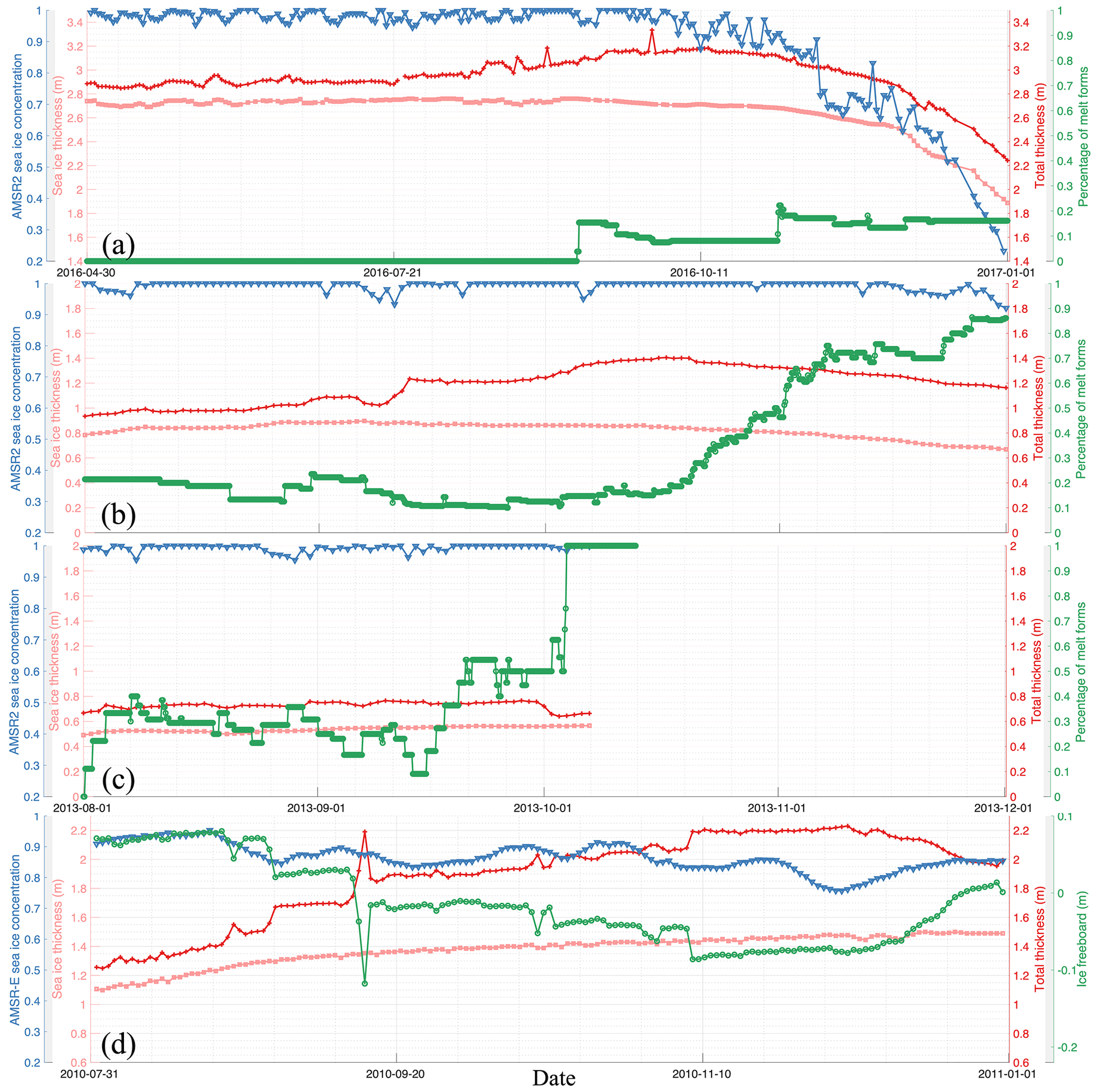
Figure 2 Sea ice and atmospheric conditions in (a) AWI 2016S31, (b) PS81/506, (c) PS81/517, and (d) ZS-2010. Sea ice thickness (light red) and total ice thickness (snow depth + sea ice thickness) (red) are collected from the buoy measurements. Sea ice concentration (blue) is from AMSR-E/2 datasets, the brine-wetted layer (melt form) percentage (green) is from the SNOWPACK model, and the ice freeboard (green) is from buoy measurements.

4 Results

4.1 Wintertime snow properties on Antarctic sea ice

4.1.1 Snow evolution from buoys

From late summer until 1 September 2016, the average early autumn snow depth at the 2016S31 buoy location remained constant at 19 cm. However, on this date, a significant snowfall event occurred, increasing the snow depth to 30 cm. By the end of September, it grew to over 50 cm, as recorded by the buoy (deduced as total thickness minus ice thickness in Fig. 2a) and as used in the SNOWPACK simulation (Fig. B1a). The snow stratigraphy simulation from SNOWPACK for each buoy location is shown in Fig. B3. Red colours correspond to locations with meltwater within the upper and middle snowpack, indicating the existence of the wetted layer. Starting from 14 September 2016, depth hoar (due to a consistent negative temperature gradient) and melt layers (due to rain and higher air temperatures) began to form, as reported by Wever et al. (2020). As a consequence, the proportion of the wet and saline snow layer, shown as green lines in Fig. 2a, increased. This led to a rise in the ice surface temperature (not depicted in the figures), attributed to the diminishing insulating effect of the snow cover. Concurrently, sea ice thickness gradually started thinning from its initial measurement of 2.78 m, continuing to thin throughout the early spring due to warm conditions.

Snow and ice remain stationary, followed by heavy snowfall (over 35 cm snow depth) starting from 11 September 2013 in PS81/506 (Fig. 2b). Throughout this period, brine-wetted layers were consistently present and became the predominant layer by mid-October. In the case of PS81/517, more extreme conditions were observed. Here, in PS81/517, thin ice (0.5 m) and thick snow (0.25 m) facilitated the formation of the brine-wetted snow layer. This process continued until the entire snow column became fully saturated.

A significant event was recorded on 15 September 2010, at the ZS-2010 buoy in Prydz Bay. A rapid increase in snow accumulation during this period resulted in the snow height reaching 0.85 m, which eventually stabilized at 0.55 m, as depicted in Fig. 2d. At the same time, flooding occurred on the ice surface, causing snow ice formation. In the following weeks, the snow cover continued to accumulate steadily, reaching a height of 0.85 m by November 2010. The most significant negative ice freeboard was measured at −0.09 m.

Figure 3 Observed distribution of (a) snow density (unit: kg m⁻³) and (b) salinity (unit: psu) within different snow stratigraphies in all 13 PS81 ice stations, with the median (white dots), 25th and 75th percentiles (thick black vertical bars), whiskers in 95 % confidence interval (thin black vertical bars), and all data (points) in the violin. (c) All measured salinity (in orange circles) and density (in purple stars) from 13 ice stations, with their average in crosses and pluses, respectively. Panel (d) is the frequency (grey bars) and relative snow height (dots) for different snow stratigraphies in all ice stations during the PS81 and SIPEX II field campaigns.

4.1.2 Snow density and salinity distribution

Figure 3 provides the density and salinity characteristics of six distinct snow types, derived from an analysis of snow pits at 13 ice stations during the period between 21 June and 2 August 2013. Further detailing can be observed in Fig. B4, which presents stratigraphic data from ice stations PS81/506 and PS81/517. The uppermost layer of the snowpack at these locations was predominantly wind slab, while the lowest layer was largely characterized by formations such as snow ice, crust, refrozen slush, depth hoar, or a layer of rounded crystals. Across the seven snow types, no statistically significant differences are observed in the median density; all observed snow densities are bounded within the 5 % and 95 % percentile range of 191.3 and 390.7 kg m⁻³, with a mean value of 278.7 kg m⁻³. However, the density of the rounded crystals and snow ice/slush, which also include salinity records, has an average of 396.7 kg m⁻³ but can exceed 600 kg m⁻³. This makes them significantly denser than the bulk mean values of 280.3 and 309.3 kg m⁻³, respectively.

While data on salinity are less frequently available than density data, the existing records highlight a notably higher salinity within rounded crystals and snow ice/slush due to flooding. These records show a median salinity value exceeding 14 psu, which is significantly higher than the overall average of 10.0 psu, falling within a range marked by the 5th percentile at 0.1 psu and the 95th percentile at 38.4 psu. Given the uniformity of our dataset and the lack of significant regional variations, we utilize the mean values of snow density and salinity as standard representations for the Southern Ocean's snow conditions. Consequently, to initially portray the brine-wetted snow in various scenarios, we select a representative density of 396.7 kg m⁻³ and salinity index of 10.0 psu for the snow ice/slush or rounded crystal layer, defining its permittivity and brine volume fraction accordingly. A detailed discussion about the choice of these bulk values and their effects can be found in Sect. 5.2.

4.1.3 Statistics of snow stratigraphy

Figure 3d depicts the frequency and relative heights of different snow stratigraphy layers observed during the winter over the Southern Ocean. The data indicate that the most common snow types are wind slab, faceted crystals, ice crust, and snow ice; these types are frequently found in the Antarctic region (Massom et al., 2001).

In contrast, decomposing and fragmented particles of snow appear less frequently during this season. The wind slab (precipitation particles), often found in the uppermost layer of the snow, mainly results from wind transportation, deposition, and packing, consequently leading to the formation of a medium- to high-density hard layer, as can be seen in Fig. 3. Beneath this layer, various types of snow, such as faceted crystals, ice crust, rounded crystals, and depth hoar, can be present, each with the potential to be located at any level within the snowpack. Although it occurs infrequently (less than 8 % of snow pits), a slush of seawater and snow is most commonly found near the bottom of the snow strata, comprising approximately the lower 20 % of the structure. These layers form intriguingly; they develop when seawater infiltrates the crevices, widening brine drainage channels, which ultimately saturate the underlying snow. The dynamic process extends beyond saturation. Another notable contributing factor to this moisture is the capillary wicking-up process, a detailed description of which can be found in Fig. 6 of Massom et al. (2001). Moreover, seawater can move laterally from cracks and floe edges (Massom et al., 2001). Consequently, the resulting slush on the sea ice undergoes freezing, transforming into saline snow ice, typically a consequence of seawater flooding. Additionally, the internal ice crusts within the snow layer (Fig. 3) are formed by internal snow melt–refreeze processes, a common feature in the Antarctic snowpack. In addition, the introduction of water (whether from melting or rain-on-snow events) can add to the complexity and inhomogeneity of the snow stratigraphy, as noted by Nandan et al. (2020).

4.2 Impacts of brine-wetted snow on the TB measurement

The study assumes that both the observations and the simulations accurately represent the average snow properties for each ice floe. We adopt the following protocol to match the buoy measurements to satellite TBs. For each buoy, we compute its daily-mean locations. The daily TB map for each daily-mean location is used to attain the TB value in the cell that contains the specific location. Then the buoy's daily measurements are matched to TBs for further comparison. Essentially, this implies that the conditions observed at the buoy location are representative of the entire grid cell, ensuring that the satellite TB data are a valid proxy for the conditions across the whole floe. This premise is crucial for aligning and comparing satellite data with in situ buoy measurements.

Figure 4 The mean of the horizontally and vertically polarized TB comparison from SMOS, with simulations by RADIS-L v1.0 and RADIS-L v1.1 along the buoy trajectories and scatter fittings in the (a) AWI 2016S31, (b) PS81/506, (c) PS81/517, and (d) ZS-2010 buoys.

Heavy snow accumulation and the formation of a brine-wetted snow layer resulted in a notable decrease in SMOS TBs. Specifically, at the 2016S31 buoy, TBs dropped from 248.5 K on 14 September 2016 to 220.2 K by 10 October, as shown in Fig. 4a. This decrease in TBs, occurring despite stable sea ice concentration (depicted in light blue in Fig. 2a), is likely attributable to the newly formed brine-wetted snow layer. In the latter part of spring (mid-November), there is a discernible decline in TBs. This trend aligns with observed changes in snowmelt, ice thickness, and ice concentration dynamics. A similar pattern is observed with the PS81/506 buoy data (refer to Figs. 4b and B3b). In early September at this location, snow accumulation exceeded 0.4 m, leading to a flooding scenario on the 0.8 m thin ice surface, which subsequently resulted in the formation of a brine-wetted layer. Due to the nearly constant ice concentration approximating 100 %, the TB reduction from 243.8 K (11 September 2013) to 226.1 K (21 October 2013) cannot be attributed to the increase in open water. Notably, the depth of the brine-wetted layer in PS81/506 (Fig. 2b) becomes more pronounced around the onset of the austral spring. This correlates with the observed decrease in TBs and an increase in surface temperatures.

In contrast, the changing TBs in PS81/517 (Fig. 4c) do not show a clear trend, despite the presence and expansion of the brine-wetted layer by late winter (as depicted in Fig. 2c). A similar situation is noted in September 2010 at the ZS-2010 buoy. Even though there are clear signs of snow ice formation, as indicated by the negative freeboard data in Fig. 2d, the changes in TBs are not distinct (refer to Fig. 4d). However, this scenario begins to change in October 2010. This period marks the start of a gradual decrease in TBs, coinciding with an increase in upper snow depth while maintaining a sea ice concentration of around 90 %. Notably, a continuous decline in TBs is observed, driven by the increasing snow depth on the ice, which reaches a height of 0.85 m by 10 October 2010. This decline precedes a phase of reduction that begins around mid-December.

4.2.1 TB validation in buoy observations

AWI snow buoy

As described in Sect. 3.2, we use RADIS-L v1.1 to simulate the TBs within 40×40 km² regions, using the sea ice thickness, snow depth, ice surface temperature from the buoys, sea ice type, sea ice concentration, and relative brine-wetted depth from SNOWPACK as input to the model (Table A1). The TB comparison between the simulation and SMOS satellite is shown in Fig. 4 along the 2016S31, PS81/506, and PS81/517 trajectories. During the austral winter of early September 2016, SMOS (represented by black lines) observed a decrease in TBs. However, the RADIS-L v1.0 model (blue lines) was unable to capture these reductions. In contrast, RADIS-L v1.1 (depicted in crimson lines) accurately simulates the TB changes. Beginning on 29 August 2016 (Fig. 4a), the TBs modelled by RADIS-L v1.1 diverge from those modelled by RADIS-L v1.0, indicating the critical role of the brine-wetted layer in simulating TBs over time. Overall, RADIS-L v1.1 shows a strong correlation with SMOS data (r² of 0.682) for this buoy. For buoy PS81/506, the accuracy of RADIS-L v1.1 is notable, with an increase in r² from 0.034 (RADIS-L v1.0) to 0.560 (RADIS-L v1.1). Notably, RADIS-L v1.1 reduces the overestimation biases seen with RADIS-L v1.0, particularly in October 2013 (Fig. 4b), which aligns with the formation of the melt layer. Although the significant improvements are not seen for buoy PS81/517, the simulated TBs still remain correlated with SMOS, with an r² of 0.252.

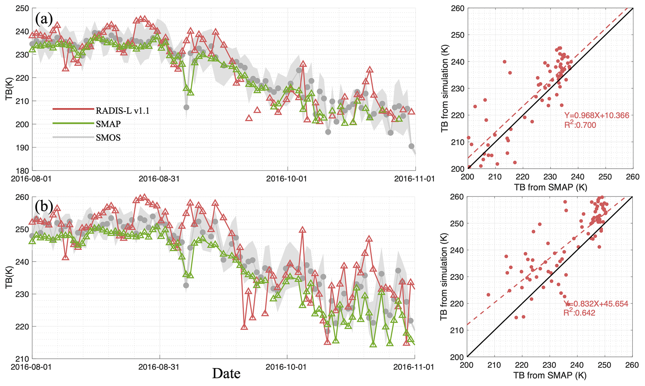
Figure 5 The (a) horizontal and (b) vertical TB comparison from the fixed incidence angle (40°) SMAP and multiple incidence angles (0–60°), as well as simulations by the RADIS-L v1.1 model along the AWI 2016S31 buoy trajectory with a scatter comparison. The shading within the SMOS observation is 1 standard deviation of multiple angles.

Furthermore, SMAP TBs are also modelled for both horizontal (Fig. 5a) and vertical (Fig. 5b) polarizations at a fixed 40° incidence angle. The grey shading represents 1 standard deviation of TBs from the SMOS RE07 product obtained from multiple incidence angles ranging from 2.5 to 62.5° at an interval of 5°. There are notable observational differences between SMOS and SMAP, especially for vertically polarized TBs, where SMOS readings are approximately 2.9 K higher than SMAP readings. Huntemann et al. (2016) also found that SMOS yielded higher TBs than SMAP in both polarizations (about 5 K). In comparison with SMAP, the simulated TBs from RADIS-L v1.1 suggest a larger bias in the vertical polarization. However, despite these positive biases and greater variability at vertical polarization, the modelled TBs maintain a high correlation with SMAP, with all r² values exceeding 0.64.

Buoys on landfast sea ice

To strengthen the validation of TBs, we have extended the dataset by incorporating detailed observations from Prydz Bay, capitalizing on the enhanced capabilities of RADIS-L v1.1. This effort involves incorporating data on sea ice thickness, snow depth, and ambient air temperature recorded by an array of SIMBA-type buoys strategically positioned throughout the bay. To further advance our research, additional data dimensions have been integrated. These include ice type classifications provided by the EUMETSAT Ocean and Sea Ice Satellite Application Facility (OSI-SAF); detailed ice concentration statistics sourced from ASI; and estimates of the brine-wetted layer depth, which are based on negative ice freeboard measurements. These additional data aspects are elaborated upon in Table A1.

In the following validation workflow, we conduct TB simulations at the location of the ZS-2010 buoy. This allows for a critical juxtaposition with SMOS measurements as illustrated in Fig. 4d. Notably, starting from mid-September, the TBs exhibit significant fluctuations. These are primarily attributed to increased snow accumulation and recurring flooding events. A comparative study between the v1.1 and v1.0 models reveals marked differences in TBs, particularly in the assessment of brine-wetted snow. The v1.1 model demonstrates a notably better fit with the observed data, characterized by a nearly perfect slope and an r² value approximating 0.36. To further validate the RADIS-L v1.1 model, we undertake a comprehensive evaluation using datasets from a series of SIMBA-type buoys deployed across Prydz Bay between 2010 and 2018, including ZS and DS buoys. Our analysis, illustrated in Fig. B7, highlights the alignment of the v1.1 model with SMOS measurements. This is evidenced by a strong correlation and a slope exceeding the 0.7 threshold, confirming our initial hypotheses and expectations.

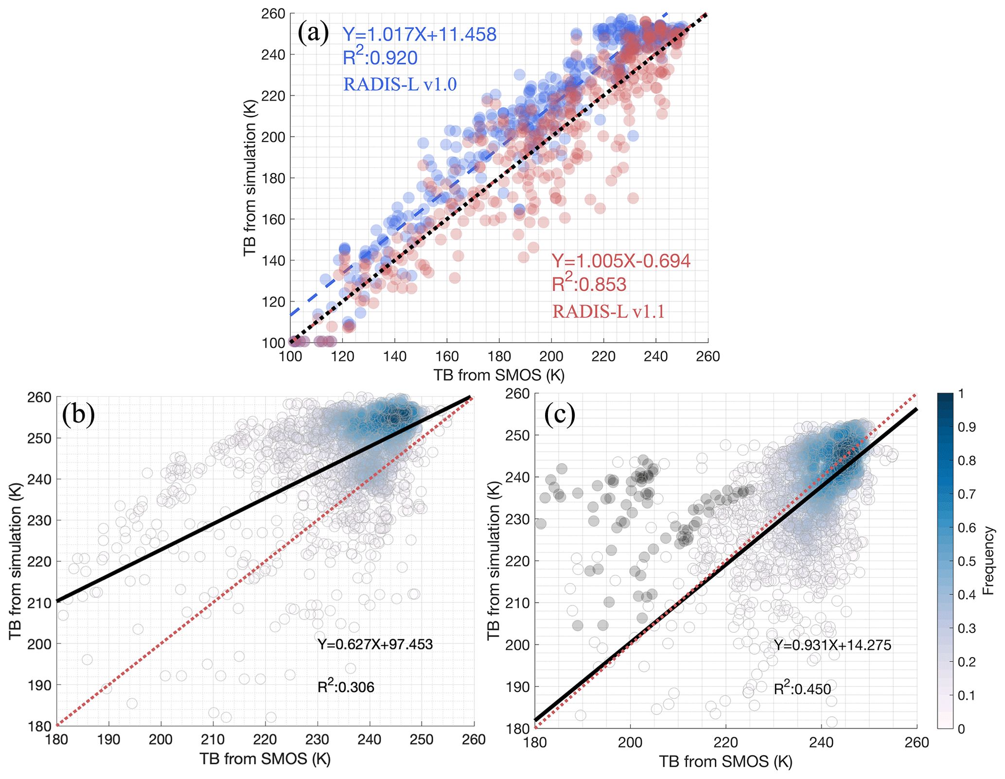
Figure 6 The TB comparison between the RADIS-L v1.1 simulation and SMOS based on (a) ASPeCt observations. Panels (b) and (c) are the heatmaps of the TB validation using all seven OIB campaigns resulting from RADIS-L v1.0 and RADIS-L v1.1. The black dots in (c) are the TB overestimation value discussed in Sect. 5.1.

4.2.2 Inter-comparison of TBs based on airborne and ship-based observations

Similar to buoy comparisons, the primary inputs for the ASPeCt-based validation encompass parameters such as sea ice thickness, snow depth, ice type, ice surface temperature, and concentration, derived from the ASPeCt single-point observation (refer to Table A1). Given the SNOWPACK limitations in non-buoy applications, we adopt negative ice freeboard as an indicator of brine-wetted snow depth. This time, ASPeCt's measurement range extends beyond the Weddell Sea to include the Bellingshausen Sea and the southern Indian Ocean, as marked by the blue squares in Fig. 1. The TBs modelled based on ASPeCt data (see Fig. 6a) align closely with those captured by SMOS. This validates the performance of both RADIS-L v1.0 (shown in blue) and RADIS-L v1.1 (in red), with the r² values exceeding 0.85. While RADIS-L v1.0 shows a marginally better correlation, RADIS-L v1.1 is notable for its lower positive bias in the simulated TBs, with the intercept decreasing from 11.5 to −0.7 K. Similar improvements are also observed in Fig. B5 when using daily-mean ASPeCt measurements as input instead of point-to-point observations in Fig. 6a.

Along the OIB tracks, TBs were simulated using OIB sea ice thickness, snow depth, KT19 ice surface temperatures, ASI sea ice concentration, OSI-SAF ice type, and brine-wetted depth determined from negative ice freeboard data (as seen in Fig. 6b and c). The snow depth (Fig. B1) from these seven campaigns shows large spatial and temporal variability. For instance, on 30 October 2010, some snow depth measurements reached as high as 2 m, with an average of 0.52±0.35 m. On 20 October 2014, snow depths peaked at 1 m, averaging 0.49±0.16 m. Meanwhile, other measurements varied between 20 and 45 cm. In terms of TB simulations, RADIS-L v1.0 tends to overestimate the SMOS TBs, with an r² of about 0.31 and a mean bias of 7.4 K. In contrast, RADIS-L v1.1 significantly reduces these overestimations, increasing the r² to 0.45 and demonstrating no statistically significant bias, although the mean of the clusters shown in Fig. 6c is approximately 1.5 K higher than that of the SMOS data. Despite these improvements, closer scrutiny of some simulations, particularly the data recorded on 28 October 2010, reveals discrepancies when compared to satellite observations. This observation suggests a need for further investigation into small-scale ice and snow surface characteristics, which can be corroborated through SAR satellite imagery and reanalysis datasets.

4.3 Examining the effects of slush snow in the SIPEX II case study

In Sect. 3.2.2, we delve into the most extreme stage of wet metamorphism after flooding: snow slush. We examine the unique impacts of slush and flooding snow within the context of brine-wetted snow layers. This analysis is based on observations from five snow and ice transects located near Wilkes Land (Fig. 1a). In this study, key attributes of slush snow, including depth, density, and salinity, are compiled into mean bulk values based on snow pit assessments. These assessments provide insightful data; for instance, the average slush snow depths at ice stations 2, 3, and 4 are found to be 3 cm, while at stations 6 and 7, the depth averages 1 cm. Across these stations, the combined mean density and salinity are calculated to be 481 kg m⁻³ and 9.83 psu, respectively.

Figure 7 The distribution of the sea ice thickness (red shading), snow thickness (blue shading), and sea ice freeboard (green stars) measurements from five transects. The violin shadings cover the range of the 1st and 99th percentiles. The upper (lower) boundaries of the slim boxes are the mean ± standard deviation, while the upper (lower) boundaries in the thick boxes are the 3rd and 1st quartiles of the parameters. The short solid horizontal lines represent the median of the observations. The purple stars, upper triangles, and lower triangles are TBs from SMOS observations and the simulations from RADIS-L v1.0 and RADIS-L v1.1 with snow ice, respectively. The crosses are the observed air temperature in each station.

Figure 7 offers valuable insights, highlighting key metrics such as air temperature, ice thickness, snow depth, and freeboard, with a focus on critical statistical values (e.g. quartile and median values). Notably, each station recorded negative freeboards. Specifically, station 4 reported the thinnest median ice thickness at 1.38 m, contrasted with a median snow depth of 0.48 m, resulting in a median negative freeboard of −0.02 m. In contrast, station 7 displayed larger median values, with an ice thickness of 4.87 m and a snow depth of 0.51 m. TB simulations, as outlined in Table A1, were systematically evaluated both with and without the slush snow parameterization. Compared to SMOS-derived TB observations (illustrated in Fig. 7), RADIS-L v1.0 simulations are consistently biased high by 8.8 K. However, this bias was significantly reduced to 2.8 K in RADIS-L v1.1, particularly after incorporating the slush snow layer, thus achieving closer alignment with the SMOS datasets, especially at stations 4 and 6. Furthermore, leveraging detailed snow morphology data from SIPEX II, the enhanced RADIS-L v1.1 model rectifies key discrepancies in existing radiation transfer models over the Southern Ocean.

Figure 8 The differences between the simulated and SMOS TBs within the 28 October 2010 track overlaid by the sea ice concentration (c) from AMSR-E and by the HH-polarized backscatter from ALOS L-band PALSAR on 29 October 2010 (a, b) and 30 October 2010 (e, f) and the (d) distribution of backscatter during these 2 d.

5 Discussion

5.1 Sub-grid-scale surface variability

On 28 October 2010, OIB flew from the corner of the Antarctic Peninsula in the northern Weddell Sea, starting at 75.0° S, 38.1° W to 64.0° S, 42.3° W (Fig. 8a). Along this flight path, notable discrepancies were observed between TBs simulated with RADIS-L v1.1 and SMOS measurements. This was particularly evident over the eastern region (marked as the grey area in Fig. B7g), where RADIS-L v1.1 overestimated the SMOS TBs by an average of 15 K. One potential explanation for this bias is that the sea ice concentration based on AMSR-E is too low, potentially influenced by atmospheric conditions. The 89 GHz channel, used in the ASI algorithm, is known to be affected by liquid cloud water. JRA55 data for 28 October 2010 indicate high atmospheric humidity and warm air temperatures (Fig. B8). Additionally, AMSR-E TBs (Fig. B7) suggest surface melting over the eastern portion of the OIB flight path.

The overestimation of sea ice concentration in the SIC product is evident from ALOS HH-polarized PALSAR backscatter over the eastern region of the OIB track on 29 October 2010 (Fig. 8a and b). The discontinued darker pixels in Fig. 8a and b represent the lower backscatter over the eastern region of the track compared to the western region (30 October 2010, Fig. 8e and f). These darker pixels suggest the presence of leads within the eastern sea ice region (brighter pixels).

Moreover, the mean SAR backscatter under the OIB footprints (Fig. 8d) shows different peaks for these two regions. On 30 October 2010, two backscatter modes were recorded at −12.4 and −14.9 dB. In contrast, on 29 October 2010, the lower mode at −20.8 dB mainly arises from leads, while the dominant peak around −13.1 dB, which constitutes over 90 % in the probability density function (PDF), corresponds to sea ice in the region.

In summary, the JRA55 atmospheric reanalysis combined with TBs from various AMSR-E bands indicates a significant presence of moisture in the air and potentially surface melt of the snow cover in the eastern section of the OIB flight path. Furthermore, visual inspection of the HH-polarized ALOS images indicates the presence of leads within the ice pack. However, the sea ice concentration product based on AMSR-E cannot directly resolve these leads, and, more importantly, it reports the SIC at 96.73±3 % within the OIB overestimation (differences >10 K) region. This is significantly higher than what the SAR image indicates. The overestimation of SIC causes positive biases in the simulated TBs compared to SMOS observations. Much lower L-band TB is usually associated with (refrozen) leads compared with the typical sea ice cover. The roles of the leads are not accounted for due to limited spatial representation by the OIB scans. This result highlights the need for including small-scale ice variability when comparing multi-scale observations of the sea ice.

Figure 9 Three configurations of the snow ice layer with different water contents (θ_w, %) and air contents (θ_a, %) in (a), (b), and (c). The total depth of the snow cover is 60 cm for all cases, while the depth of the snow ice layer is relative to that of the brine-wetted snow layer. Panel (d) is simulated TBs (unit: K) changing with different snow ice depths (%) under different slush properties (dashed and dotted lines) and the percentage of overlaid brine-wetted layer (different colours). The four horizontal lines represent the simulated TBs in different brine-wetted layer depths without the snow ice layers.

5.2 Snow ice layer and flooding effects

For a more accurate representation of snow structures around Antarctica, a detailed four-layer configuration is ideal for investigating the effects of snow ice on surface radiative properties. This configuration includes dry snow atop a brine-wetted layer followed by a snow ice layer and, finally, a sea ice layer at the bottom. As explained in Sect. 3.2.2, we consider three distinct scenarios (illustrated in Fig. 9a–c: Scenarios I, II, and III) with varying water and air properties within the snow ice layer. The snow ice layer depth here is determined by the percentage of snow ice within the brine-wetted snow. We also construct the snow ice layer with different brine-wetted snow depths (20 %, 40 %, 60 %, and 80 % of the entire snow depth). With a constant ice thickness of 2.0 m and snow depth of 0.6 m, the simulated TB is 258.2 K in the absence of any brine or snow ice layers. The inclusion of brine-wetted layers results in lower TBs, decreasing to 257.3, 256.9, 255.3, and 252.6 K as the brine-wetted snow depth increases. The inclusion of the snow ice layer further reduces the TBs depending on the snow ice properties. Here, we found that higher water content, lower air content, and hence higher density in the snow ice result in higher simulated TBs (Fig. 9d), making the TBs more akin to ice than to snow. Figure 9d also explores the TB changes under different snow ice depths for each scenario. A larger snow ice depth reduces the simulated TBs due to a decrease in snow ice temperature, resulting from less insulation provided by shallower dry snow. Moreover, as the snow ice layer thickens, the TBs decrease more significantly in Scenario I (with the least snow wetness) and in the deepest brine-wetted snow layer (80 %) compared to other scenarios. Specifically, in Scenario III (with the wettest snow), as the snow ice layer increasingly occupies the brine-wetted snow layer up to 100 % of the total snow depth, the simulated TBs converge to a consistent value of 224.5 K. However, the TBs from other wet snow ice layers (Scenarios I and II) vary when the whole brine-wetted layer is snow ice. For example, in Scenario I, the final TBs range from 183.9 to 187.1 K. Therefore, more water content in the snow ice results in less sensitivity to the snow ice depth. It is clear that the increasing depth of the snow ice layer or the decreasing depth of the brine-wetted layer corresponds to a non-linear reduction in TBs in Fig. 9d. Additionally, with the same proportion of the snow ice layer, the spread of TBs among different depths of the brine-wetted layer becomes more pronounced in scenarios with less water content in the snow ice. However, since freshly formed slush and snow ice are not explicitly distinguished here, more work is needed to deepen our understanding of the snow–slush–snow ice transformation, including the diurnal temperature development in snow on ice and its impact on the initial slush thickness and porosity (Nomura et al., 2018; Zhaka et al., 2023).

To conclude, simulations incorporating a more complex snow stratigraphy, including a snow ice layer, further reduce the modelled L-band TBs, highlighting the importance of accurately representing snow layers in such models.

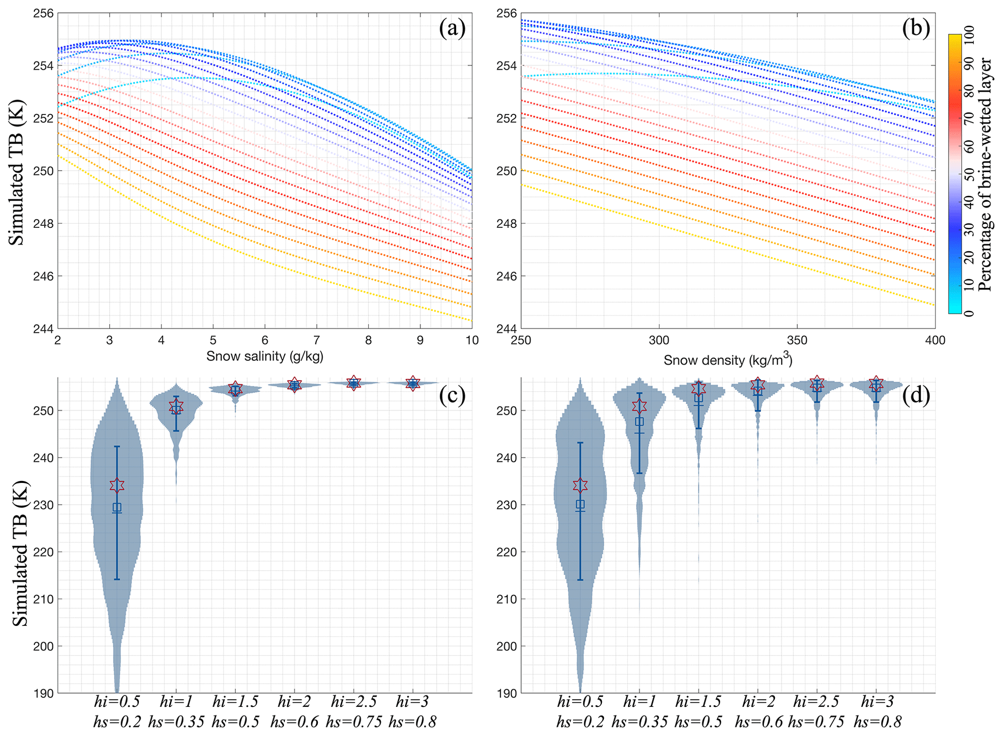
Figure 10 TB distribution under the perturbation of (a) salinity (unit: g kg⁻¹) and (b) snow density (unit: kg m⁻³). Panels (c) and (d) are under the constant (value-increased) ice and snow standard deviation Monte Carlo perturbation in the violin distribution. The stars are the TB values in single ice and snow measurements based on RADIS-L v1.1.

5.3 Sensitivity in bulk parameters

The primary default settings used in the RADIS-L v1.1 simulations are snow density and salinity from the in situ measurements around the Southern Ocean. The following examines the effects and sensitivity from using these bulk values and the schemes of sampling in the TB simulations.

Figure 10a and b denote the TB values for different snow densities, salinity, and percentage of brine-wetted snow layers for a 2 m thick ice floe covered by 0.6 m of snow. The snow density and salinity are chosen within the 5 % and 95 % range of PS81 ice station measurements. Figure 10 suggests that snow salinity and density are inversely correlated to L-band TBs. Specifically, TBs decrease by approximately 4.5 K with an increase in snow density from 250 to 400 kg m⁻³. Similarly, TBs reduce by more than 5 K when snow salinity increases from 2 to 10 g kg⁻¹. Notably, the impact on L-band TBs from changes in snow salinity is more pronounced than that from density. This can be attributed to the greater variation in the complex dielectric constant of brine-wetted snow due to salinity, as illustrated in Fig. B9. Furthermore, the extent of TB reduction is influenced by the percentage of brine-wetted depth within the snow. Generally, a higher percentage leads to a greater reduction in TBs. However, for thinner brine-wetted layers, the relationship between snow properties and TBs exhibits non-monotonic (convex) curves. The most likely explanation is that the low conductivity, attributed to the needlelike shape of brine inclusions within the thin brine-wetted layer, disrupts the connectivity of these inclusions (Geldsetzer et al., 2009), resulting in higher temperatures within the snow. Furthermore, the permittivity of that layer becomes highly sensitive to temperature variations around −8 °C (Morey et al., 1984), exhibiting larger TB variabilities in thinner layers (as shown in the notching curves between temperature and the dielectric constant in Fig. B9). This results in increased sensitivity of TBs. The non-monotonic relationship between microwave observations and the impact of snow salinity remains an open area for discussion and warrants further investigation.

One phenomenon deserves attention: when the brine-wetted layer is thinner than 20 % of the entire snow depth, TBs can be lower than those from thicker brine-wetted layers. However, additional research is needed to fully understand the effects of brine-wetted layer characteristics on L-band TBs. Further exploration demands more detailed data, including a deeper understanding of the significant influence regional-dependent snow density and thermal conductivity exerts on sea ice growth, as referenced in Arndt (2022). However, such an extensive inquiry lies beyond the scope of this study.

In addition to the study regarding the sensitivity of default parameters, we also examine the sampling schemes, i.e. one or multiple sea ice samples (Fig. 10c and d). Here, a set of 6000 samplings is generated under the context of (i) constant standard deviation (SD) for snow depth and ice thickness (${\mathrm{SD}}_{h_{\mathrm{i}}}=\mathrm{0.3}$ m, ${\mathrm{SD}}_{h_{\mathrm{s}}}=\mathrm{0.1}$ m) and (ii) mean value-dependent (deduced from OIB measurements) standard deviation of ice and snow (${\mathrm{SD}}_{h_{\mathrm{i}}}=\mathrm{0.63}\times h_{\mathrm{i}}$, ${\mathrm{SD}}_{h_{\mathrm{s}}}=\mathrm{0.36}\times h_{\mathrm{s}}$) through Monte Carlo lognormal distribution perturbations. By applying these sampling schemes across various ice thickness and snow depth scenarios, we present the simulated TBs for five sea ice and snow conditions using violin plots in Fig. 10. The blue squares and the three horizontal lines (Fig. 10c and d) represent the medians, means, and ± standard deviations in simulated TBs following the Monte Carlo perturbations. Meanwhile, the orange stars indicate the TB values from the mean h_i and h_s (representing a single sampling condition). The constant SD perturbation (Fig. 10c) indicates that only one sample always overestimates the average of TBs, especially over thin ice; these biases would be negligible over the thick ice. Similarly, value-dependent sampling (Fig. 10d) demonstrates the biases from significant overestimation to minor underestimation when ice thickness increases. This type of sampling depicts a more realistic lognormal distribution of TBs compared to the constant SD scheme. Thus, this sensitivity study suggests that more measurements or observation inputs would improve the accuracy in simulated TBs or other passive microwave parameters. Moreover, thick ice and snow are less susceptible to issues of undersampling. Thus, the drastic decline in sea ice thickness in the 21st century for both the Arctic and the Antarctic (Mallett et al., 2021; Kacimi and Kwok, 2022) will continue to challenge the validity of microwave satellite remote sensing retrievals. This challenge is particularly pronounced if the algorithms rely predominantly on a limited number of sea ice measurements for training and calibration.

6 Conclusions

In this research, we examine the nuanced effects of Antarctic snow stratigraphy on the radiative attributes of ice surfaces, with a particular focus on brine-wetted and slush/snow ice layers. By incorporating advanced parameterizations in RADIS-L v1.1, we have achieved significant advancements in accurately representing observed ice surface TBs. This progress establishes a solid basis for more precise future research and applications in the realm of polar ice surface studies.

The substantial snow cover and complex snow–ice interaction in Antarctica often lead to basal snow having high salinity and moisture content. This frequently entails ice surface flooding or the formation of snow ice, not limited to the snow–ice interface, as indicated by Webster et al. (2018). Utilizing data from AWI- and SIMBA-type buoys, as well as simulations from SNOWPACK, we observed a progressive increase in the extent of the brine-wetted layer, especially as the ice becomes increasingly overburdened. Interestingly, this phenomenon of ice flooding is also evident in landfast ice regions. Often, this flooding is either temporally coincident with or preceded by ice breaking and a reduction in ice concentration, highlighting the link between declines in TBs and changes in the thickness and/or vertical extent of the brine-wetted layer (less thermal insulation). Consequently, we have incorporated the thermal conductivity and permittivity of brine-wetted snow, which differ from those of dry snow, into the RADIS-L v1.1 model. To validate our improved parameterization, we used existing extensive sea ice measurements from the Southern Ocean, encompassing data from airborne platforms, in situ buoys, and ship trajectories. We then compared these simulated TBs with satellite data from both SMOS and SMAP. By integrating the atmospheric-reanalysis-driven prognostic model SNOWPACK with the diagnostic radiation model RADIS-L v1.1, we are able to demonstrate, for the first time, the critical role of the brine-wetted snow layer in understanding the changes in radiative properties of ice surfaces at L-band frequencies.

In particular, the large sensitivity of modelled L-band surface TB values to the presence of open water requires us to work with sea ice concentration datasets of an as fine as possible spatial resolution – such as SAR-based ones as suggested by Ludwig et al. (2019). Our ongoing research aims to integrate these merged and high-resolution datasets to refine the accuracy of snow depth retrieval from microwave satellites. Additionally, the integration of a detailed slush layer into RADIS-L v1.1 has proven to be crucial, significantly reducing the simulated TBs in a manner closely linked to the properties of the snow ice layer such as thickness and brine volume. This finding highlights the complexity of accurately simulating TBs for thin brine-wetted snow layers and emphasizes the urgent need for detailed research to unravel the intricate relationships between snow salinity, density, and TBs, particularly in the context of thicker layers.

The urgent need for detailed laboratory and field research is clear, especially in untangling the complexities of brine-wetted and snow ice layers, which are particularly prevalent in the Southern Ocean. In this region, data on such phenomena are still sparse. The scenarios we have discussed provide critical benchmarks for improving radiometer designs, as well as their calibration and validation processes in various settings. Recognizing the limitations posed by undersampled measurements is crucial; such limitations can significantly impact the precise retrieval of ice parameters and the fine-tuning of algorithms used in L-band satellite imagery, most notably in regions with thinner ice. These limitations are particularly concerning in light of climate change and its impacts. Therefore, it is vital to enhance our data collection with consistent, detailed observations from ground-based sources, aerial surveys, and field research. Strengthening our data collection is essential for maintaining the accuracy and reliability of satellite observations in tracking and understanding changes in polar regions.

The accuracy and statistical parameters of ship observations, such as those from ASPeCt, vary based on factors like the observers' subjective judgements, observation techniques, time of the expedition, and the ships' routes. For example, the ships tend to stay in easily navigable water, inducing preferential sampling and underestimation of both the sea ice concentration and the thickness (Worby et al., 2008; Weissling et al., 2009). In this study we mainly utilize available data from ASPeCt to broaden the coverage in the vast area of the Southern Oceans. The limitations for using ship-based measurements for model validation need to be examined in detail, especially the effect of uncertainties in the sea ice and the snow thickness parameters.

Finally, building upon the successes of heritage missions like AMSR and SMOS- and SMAP-type missions, the high-priority candidate mission, the Copernicus Imaging Microwave Radiometer (CIMR) (planned to launch in 2025+ by ESA: http://www.cimr.eu/, last access: 19 September 2024), aims to provide microwave imaging radiometer measurements across a broad spectrum, from 1.4 to 36.5 GHz, encompassing L-, C-, X-, Ku-, and Ka-bands (Scarlat et al., 2020). Several studies (Kilic et al., 2020; Jiménez et al., 2021) have already stated the potential performance of the CIMR instrument and estimated the retrieval precision, including different sea ice parameters. Therefore, the algorithms and findings presented in this paper have promising applications for simultaneous and consistent ice parameter retrievals using CIMR, considering the high-frequency coverage, improved spatial resolution, and high radiometric precision. The CIMR mission is expected to facilitate a more comprehensive understanding and retrieval of complex snow stratigraphy and properties over sea ice at both poles. This will be invaluable for further development and validation of algorithms, contributing significantly to our understanding of polar regions.

Appendix A: Supplementary table

(Wever et al., 2020)(Wever et al., 2021a)

Table A1 Input parameters and their sources in the RADIS-L v1.1 model. OBS is the abbreviation of direct observations.

^* Observed depth, density, and salinity of snow ice from five ice stations are used to simulate the TBs in Sect. 4.3.

Appendix B: Supplementary figures

Figure B1 Snow depth (unit: m) retrieved from NSIDC L4 datasets during 2010 OIB campaigns and from the average of wavelet and peakiness algorithms during 2011–2016 OIB campaigns.

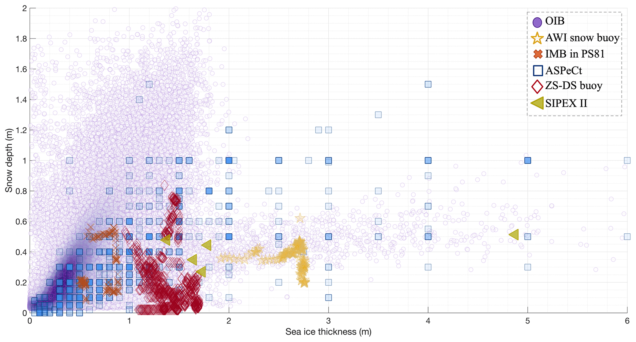
Figure B2 All measured sea ice thickness (unit: m) and snow depth (unit: m) from OIB campaigns, the AWI snow buoy, the PS81 expedition, and ASPeCt.

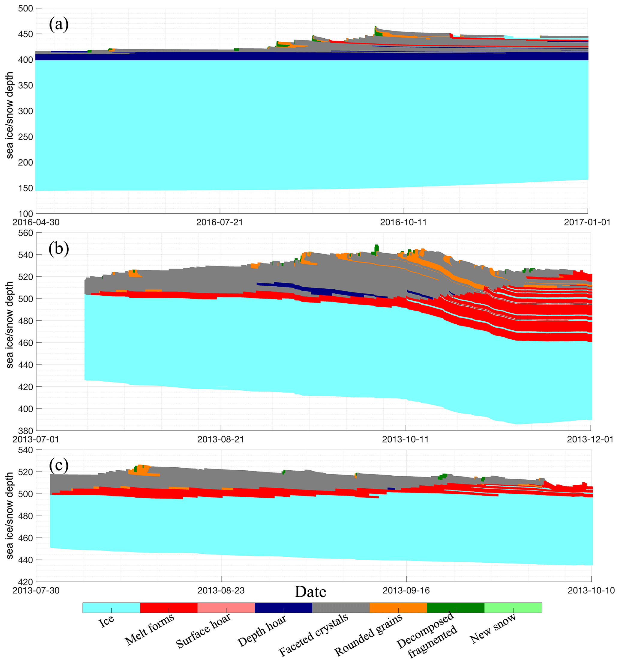
Figure B3 Snow stratigraphy modelled from the SNOWPACK in (a) AWI 2016S31, (b) PS81/506, and (c) PS81/517.

Figure B4 Observed snow density (unit: kg m⁻³) within different snow stratigraphies in the ice stations (a) PS81/506 and (b) PS81/517.

Figure B5 Validation of TBs between the RADIS-L v1.1 simulation and SMOS, based on daily-mean ASPeCt measurements, as contrasted by point-to-point ASPeCt measurements in Fig. 6a.

Figure B6 TB validation between simulation from RADIS-L v1.1 and SMOS based on all 10 SIMBA-type buoy measurements over Prydz Bay.

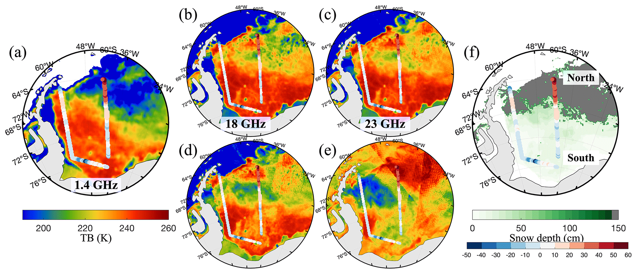
Figure B7 The TB differences (circles, coloured red to blue) between the RADIS-L simulation and SMOS observation for the 28 October 2010 track, overlaid with (a) SMOS (1.4 GHz) and different AMSR-E frequencies from 18–89 GHz (b to e). The snow depth map (f) is obtained from AMSR-E products.

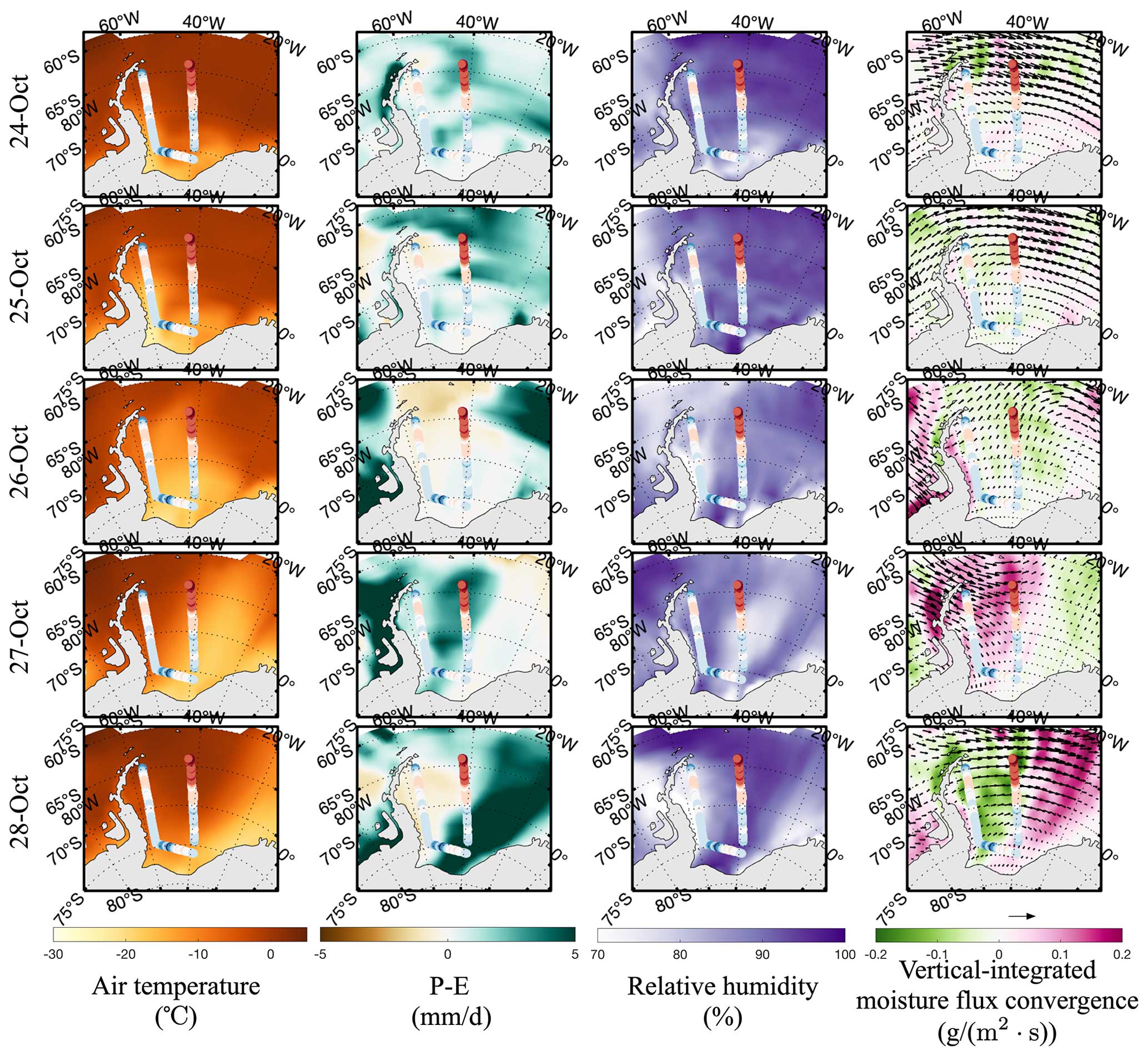
Figure B8 Atmospheric condition over air temperature (unit: °C), net precipitation (P-E; unit: mm d⁻¹), relative humidity (%), and vertical-integrated (700–1000 hPa) moisture flux convergence (unit: g m⁻² s⁻¹) during the period between 24 October 2010 and 28 October 2010.

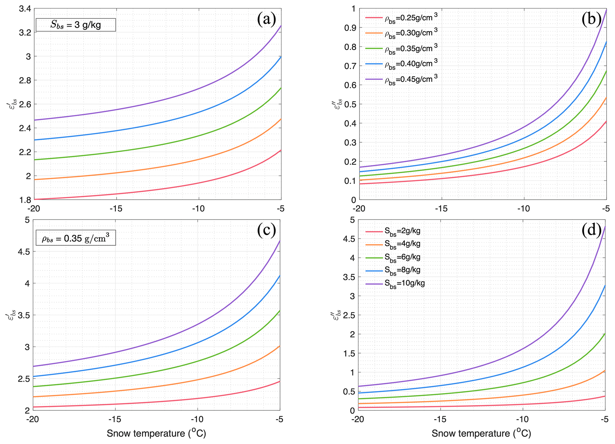
Figure B9 Real (${\mathit{\epsilon }}_{\mathrm{bs}}^{\prime }$: a, c) and imaginary (${\mathit{\epsilon }}_{\mathrm{bs}}^{\prime \prime }$: b, d) parts of the complex dielectric constant of brine-wetted snow changes with the snow temperature for different snow densities (constant: S_bs=3 g kg⁻¹, a, b) and salinities (constant: ρ_bs=0.35 g cm⁻³, c, d).