the Creative Commons Attribution 4.0 License.
the Creative Commons Attribution 4.0 License.
 | 19 Sep 2024
Multiscale modeling of heat and mass transfer in dry snow: influence of the condensation coefficient and comparison with experiments
Neige Calonne
Frédéric Flin
Christian Geindreau
Temperature gradient metamorphism in dry snow is driven by heat and water vapor transfer through snow, which includes conduction/diffusion processes in both air and ice phases, as well as sublimation and deposition at the ice–air interface. The latter processes are driven by the condensation coefficient α, a poorly constrained parameter in the literature. In the present paper, we use an upscaling method to derive heat and mass transfer models at the snow layer scale for values of α in the range 10−10 to 1. A transition α value arises, of the order of 10−4, for typical snow microstructures (characteristic length ∼ 0.5 mm), such that the vapor transport is limited by sublimation–deposition below that value and by diffusion above it. Accordingly, different macroscopic models with specific domains of validity with respect to α values are derived. A comprehensive evaluation of the models is presented by comparison with three experimental datasets, as well as with pore-scale simulations using a simplified microstructure. The models reproduce the two main features of the experiments: the non-linear temperature profiles, with enhanced values in the center of the snow layer, and the mass transfer, with an abrupt basal mass loss. However, both features are underestimated overall by the models when compared to the experimental data. We investigate possible causes of these discrepancies and suggest potential improvements for the modeling of heat and mass transport in dry snow.
- Article
(5887 KB) - Full-text XML
-
Supplement
(559 KB) - BibTeX
- EndNote


Natural snowpacks are frequently subjected to temperature gradients induced by meteorological conditions. In the case of temperature gradient in dry snow, heat and water vapor are transported through the snowpack by heat conduction through ice and air and by vapor diffusion in air. These phenomena are coupled by the sublimation–deposition processes at the ice–air interfaces. In practice, such transfer processes can be enhanced by natural air convection induced by the temperature gradient (e.g., Jafari et al., 2022) or by forced convection generated by the wind at the snowpack surface (e.g., Albert and McGilvary, 1992; Calonne et al., 2015). For the sake of simplicity, both types of convection are neglected in the following. All those processes lead to changes in the snow microstructure called the temperature gradient metamorphism (TGM), which transforms snow into faceted crystals (FC) in the case of moderate gradients and into depth hoar (DH) for stronger gradients (see Fierz et al., 2009). Those transformations of the microstructure can sometimes come along with a redistribution of mass in the snow layer, a density drop, or even the formation of an air gap at the base of the snowpack, as observed in the Arctic (e.g., Domine et al., 2019) or in some cold room experiments (e.g., Kamata and Sato, 2007; Wiese, 2017; Bouvet et al., 2023). As a result of changes in microstructure and density, the TGM also induces significant changes in the snow physical and mechanical properties, such as thermal conductivity, vapor diffusivity, or elastic properties (e.g., Srivastava et al., 2010; Calonne et al., 2014a; Wautier et al., 2015), affecting the snowpack behavior at larger scale. Hence, an accurate representation of the heat and mass transport processes during the TGM is key to accurately model the snow cover, as required for many applications such as avalanche forecasting or climate studies (Jordan, 1991; Lehning et al., 2002; Vionnet et al., 2012).
Models to describe the heat and mass transfer at the pore scale, referred to as the micro-scale, have been proposed (e.g., Flin et al., 2003; Flin and Brzoska, 2008; Kaempfer and Plapp, 2009; Vetter et al., 2010; Bouvet et al., 2022). Based on explicit representations of the 3D snow microstructure, often from X-ray tomography images, simulations at that scale are usually performed on small snow volumes due to numerical cost limitations. In micro-scale modeling, heat and mass transfer processes are coupled through interface conditions that account for the sublimation and deposition processes at the air–ice interface and involve an interface growth velocity. In snow physics, the interface growth velocity is classically given by the Hertz–Knudsen equation and strongly depends on the condensation coefficient α, also called attachment, sticking, deposition, or kinetic coefficient (e.g., Flin et al., 2003; Libbrecht, 2005; Brzoska et al., 2008; Kaempfer and Plapp, 2009; Furukawa, 2015; Krol and Löwe, 2016; Fourteau et al., 2021a; Granger et al., 2021). This coefficient describes the probability that a water vapor molecule striking the ice surface will be incorporated into it and that it theoretically ranges from 0 to 1 for an infinite flat surface (see, e.g., Libbrecht, 2005; Furukawa, 2015). The analogous coefficient for sublimation can also be defined but is often assumed equal to the condensation coefficient. At present, the condensation coefficient is still poorly understood and quantified, notably because of its complex dependencies on temperature, supersaturation (or temperature gradient), and ice crystalline orientation (see, e.g., Libbrecht, 2021). Estimates of the condensation coefficient can be found in the literature. Typical values obtained from single-ice-crystal growth experiments range from 10−4 to 10−1 (see, e.g., Libbrecht and Rickerby, 2013). Indirect estimates from snow modeling at the pore scale range from 10−4 to 10−3 (see, e.g., Flin, 2004; Bouvet et al., 2022).
In the last few decades, several models have been presented to describe the heat and mass transfer at the scale of a snow layer, referred to as the macro-scale. At that scale, the snow microstructure is not explicitly represented, and simulations can be carried out on entire snowpacks. The first models assumed saturated vapor conditions in the snow (e.g., de Quervain, 1963; Anderson, 1976; Powers et al., 1985). Later, using a phenomenological approach, Albert and McGilvary (1992) proposed describing the heat and water vapor transfer through a snowpack subjected to an airflow but without restricting the water vapor to its saturation value. The model uses two coupled advection–diffusion equations, including a source term arising from phase change at the pore scale. A similar heat and mass transfer model was analytically obtained by Calonne et al. (2014b, 2015), using an upscaling method. In that case, the macroscopic equivalent modeling was derived from its description at the pore scale using the homogenization of multiple-scale expansions. This theoretical method also provides the exact expression of the effective parameters arising at the macro-scale and the domains of validity of the macroscopic modeling. Two main effective parameters emerge from the model: (i) the effective thermal conductivity keff, which depends on the ice and air conductivity and on the snow microstructure, and (ii) the effective diffusion Deff, which depends on the vapor molecular diffusion coefficient and the snow microstructure. The source term is related to the Hertz–Knudsen equation, which involves the condensation coefficient α. Calonne et al. (2014b) have shown that this model is valid for interface growth velocities below 3 × 10⁻¹¹ m s−1, which typically corresponds to slow kinetics.
Other approaches largely rely on the assumption of saturated vapor conditions, which seems valid for faster kinetics and rather high values of α (e.g., Sturm and Benson, 1997; Kamata and Sato, 2007; Hansen and Foslien, 2015). Hansen and Foslien (2015) developed a heat and mass transfer model using a mixture theory. Assuming that the water vapor is saturated (based on the value of α=0.0144 from Delaney et al. (1964)), the authors derived a unique thermal equation which yields an apparent thermal conductivity that depends on the air and ice conductivities, the water vapor diffusivity, the latent heat of sublimation–deposition, and the temperature derivative of the Clapeyron equation. A similar formulation of the apparent thermal conductivity was also proposed by Yosida et al. (1955). Recently, Fourteau et al. (2021b) investigated the influence of α on the apparent diffusion coefficient in snow. By performing numerical simulations on 3D images, they showed that this apparent diffusion coefficient is equal to Deff for α values smaller than and then increases with increasing α until it reaches a plateau for α values larger than 10−2, with the value at the plateau smaller than the molecular diffusion of water vapor in the air. In a companion paper, Fourteau et al. (2021a) computed from 3D images the apparent thermal conductivity of snow, assuming that the water vapor at the ice–air interface is equal to the water vapor at the saturation point given by the Clapeyron equation. In this case, they showed that the apparent thermal conductivity is enhanced by the sublimation–deposition process arising at the pore scale. Their results are consistent with the model of Moyne et al. (1988) for wet porous media, based on the same hypothesis at the micro-scale and derived using the volume averaging method.
Further uses of the abovementioned models, as well as their implementation in full snow cover models, are limited by some challenges. One is the difficulty in choosing between models, as they differ in many ways. They were derived using different methods; involve different balance equations and effective parameters; and are valid for different, often unclear, domains of validity in terms of α values. This should be clarified, especially by estimating the α values for which the assumption of saturated water vapor is theoretically valid. A second challenge is that none of these models was thoroughly evaluated to assess their performances. This might be partly due to the limited number of suited datasets to compare with. The datasets from the cold-laboratory experiments of Kamata and Sato (2007) and, recently, of Bouvet et al. (2023), however, seem appropriate for such comparisons, as they provide the time series of the vertical profiles of snow density and temperature, as well as the forcing conditions to be reproduced in the simulations.
This paper aims (i) to define the heat and mass transport modeling in dry snow for the full range of α values and (ii) to evaluate the model's ability to reproduce natural snow evolution during the TGM. To this end, first, the homogenization of multiple-scale expansions is applied to derive the macroscopic equivalent modeling of heat and vapor transfer for α values ranging from 10−10 to 1, following Calonne et al. (2014b). The physics considered at the pore scale includes heat conduction, vapor diffusion, and phase change and neglects any transport linked to the curvature effect and convection. The macroscopic models and the involved macroscopic properties are compared to the ones from the literature and are illustrated for simplified snow microstructures. Second, the derived macroscopic models are evaluated using three cold-laboratory experiments of TGM from Kamata and Sato (2007) and Bouvet et al. (2023). The experiments are reproduced with the macroscopic models, and results between observations and simulations are analyzed.
2.1 Upscaling method
We apply the homogenization technique of multiple-scale expansions (Bensoussan et al., 1978; Sanchez-Palencia, 1980) to the physics of heat and vapor transport in dry snow. The homogenization method allows us to model the local physical processes in heterogeneous media by an equivalent continuous macroscopic description if the condition of separation of scales is satisfied (Bensoussan et al., 1978; Sanchez-Palencia, 1980; Auriault, 1991; Auriault et al., 2009). This separation of scales can be expressed as , where l and L are the characteristic lengths of the heterogeneities at the pore scale and of the macroscopic sample or excitation, respectively. This condition implies the existence of a representative elementary volume (REV) of size l for both the material and the excitation. Following the methodology presented by Auriault (1991), the macroscopic equivalent model is obtained from the description of the physics at the pore scale by (i) assuming the medium to be periodic, without the loss of generality, as the condition is fulfilled; (ii) writing the description of the physics at the pore scale in a dimensionless form; (iii) evaluating the obtained dimensionless numbers with respect to the coefficient of separation of scale ε; (iv) looking for the unknown fields in the form of asymptotic expansions in powers of ε; and (v) solving the successive boundary value problems that are obtained after introducing these expansions in the pore-scale dimensionless description. The macroscopic equivalent model is obtained from compatibility conditions that are the necessary conditions for the existence of solutions to the boundary value problems.
2.2 Physical processes at the pore scale
As in Calonne et al. (2014b), we assume that a snow layer of the characteristic length L can be represented by a collection of spatially periodic REVs of the characteristic length l, such that the coefficient of separation of scale .
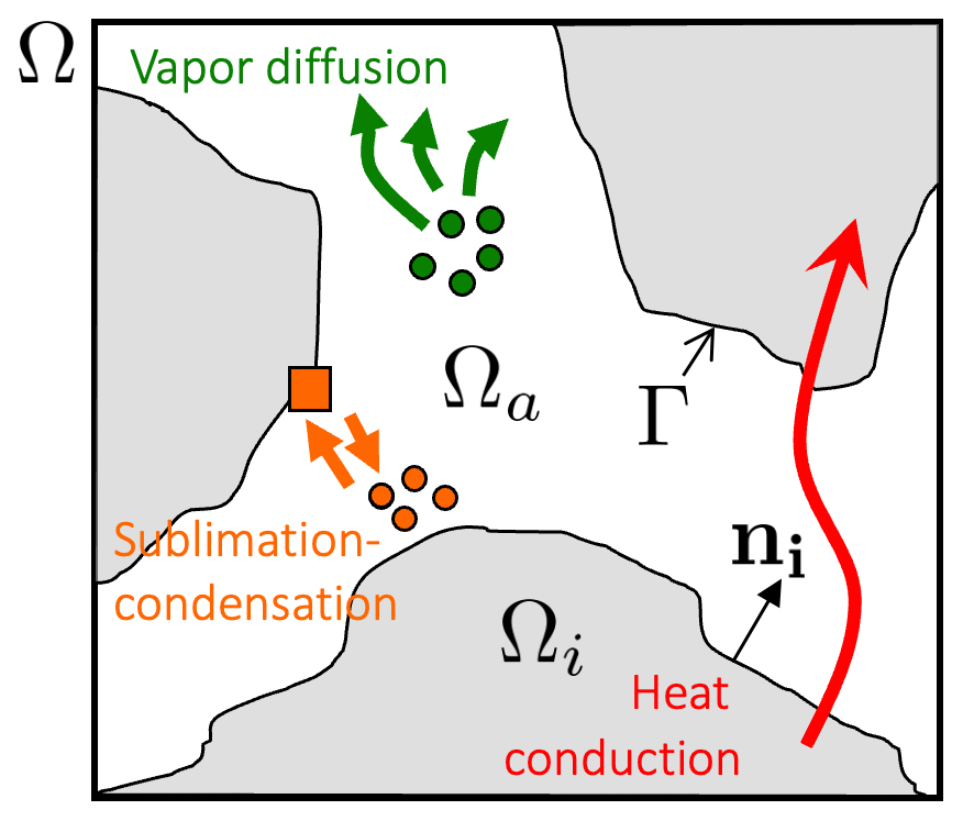
Figure 1Physical phenomena under consideration at the representative elementary volume (REV) scale.
In what follows, Ω is the REV domain, Ωi is the ice domain, and Ωa is the air domain (Fig. 1). The ice grain interface is denoted Γ, and ni is the unit's outward vector of Ωi. The subscripts i or a are related to quantities defined in Ωi and Ωa, respectively. As illustrated in Fig. 1, the processes of heat and mass transport in dry snow considered are (i) the heat conduction through ice and air; (ii) the water vapor diffusion in air; and (iii) the sublimation of ice and the deposition of vapor at the ice grain interface, characterized by an interface growth velocity (Libbrecht, 2005; Kaempfer and Plapp, 2009; Barrett et al., 2012), following the Hertz–Knudsen equation. This latter equation, initially derived to describe the condensation–evaporation processes at a liquid–gas interface, is widely used in snow physics and is supported by a great deal of experimental evidence (e.g., Libbrecht, 2005; Kaempfer and Plapp, 2009; Furukawa, 2015; Libbrecht and Rickerby, 2013; Krol and Löwe, 2016. Air convection and snow densification are not taken into account here. Assuming that the properties of air and ice are isotropic, these physical processes at the pore scale are described by the following set of equations:
where t is the time (s), T is the temperature (K), k is the thermal conductivity (W m−1 K−1), ρ is the density (kg m−3), C is the specific heat capacity (J kg−1 K−1), Lsg is the latent heat of sublimation–deposition (J m−3), w is the interface growth velocity (m s−1), ρv is the partial density of water vapor in air (kg m−3), Dv is the water vapor diffusion coefficient in air (m2 s−1), and div and grad are the divergence and gradient operators with respect to the physical space variable X, respectively. At the interface, the heat and mass transfer are coupled through the normal interface growth velocity, , which is given by the Hertz–Knudsen equation,
such that wn is positive when the ice grain grows and negative when it sublimates. β is the interface of the kinetic coefficient (s m−1), ρvs is the saturation of the water vapor density in air (kg m−3), d0 is the capillary length (m), and K is the interface of the mean curvature (m−1). The interface kinetic coefficient β is linked to the condensation coefficient α by
where m is the mass of a water molecule (kg), and kB is the Boltzmann constant equal to 1.38 × 10⁻²³ J K−1. As already mentioned, the condensation coefficient α characterizes the probability of a water molecule hitting the surface of the solid to be incorporated to the crystal, or vice versa, and ranges from 0 to 1. Although this coefficient depends on several parameters as temperature, supersaturation, and crystalline orientation, we assume that this parameter is constant over the REV at the first order. The saturation vapor density ρvs at a given air temperature Ta is given by the Clausius–Clapeyron law as follows:
In the current work, we chose the reference values Tref=263 K, leading to a value of 2.173 × 10⁻³ kg m−3. For simplicity, we assume that none of the material properties (ρ, C, kB, Dv, β, and m) depend on the temperature. Also, the effect of curvature on the ice interface growth is considered insignificant compared to the effect of temperature and is thus neglected. Consequently, using Eq. (8), the Hertz–Knudsen equation can be rewritten as
where is defined as a kinetic velocity which depends on the temperature at the ice–air interface. Taking this result into account, Eqs. (5) and (6) can be rewritten as
2.3 Dimensionless pore-scale description
The next step is the normalization of the above pore-scale description in Eqs. (1)–(4) and (11)–(12). For that reason, all the dimensional variables in this description are written such that each variable φ reads , where the subscript c denotes a characteristic quantity (constant), and the asterisk superscript denotes a dimensionless variable. Note that the microscopic length l is chosen as characteristic length, such that lc=l; i.e., the so-called microscopic point of view is adopted (Auriault, 1991). The formal dimensionless set of equations that describes the physics at the pore scale can thus be written as
This dimensionless description introduces seven dimensionless numbers that characterize the relative intensity of the physical processes at the pore scale. These dimensionless numbers are defined as
Dimensionless numbers and correspond to the inverse of the Fourier number in Ωi and Ωa, respectively. They characterize the ratio between the thermal energy storage rate and the heat conduction rate. is an analogous inverse Fourier number for the transient water vapor transfer by diffusion in Ωa. Dimensionless numbers [K], [R], [H], and [WR] are defined at the ice–air interface. [H] characterizes the ratio between the heat flux induced by deposition and sublimation and the heat flux induced by conduction in the air phase. The above analysis differs slightly from the one presented in Calonne et al. (2014b). Indeed, two new dimensionless parameters are introduced, [WR] and [R], to better capture the effect of α on the macroscopic models. Finally, let us remark that Eq. (18) defined at the ice–air interface corresponds to a Robin boundary condition, i.e., a weighted combination of a Dirichlet boundary condition and a Neumann boundary condition. Hence, when [WR] tends towards zero, Eq. (18) is equivalent to a Neumann boundary condition (), whereas when [WR] tends towards infinite (or is very large), Eq. (18) is equivalent to a Dirichlet boundary condition ().
2.4 Estimation of the dimensionless numbers
The next key step is to estimate the above six dimensionless numbers with respect to the separation of scale parameter in order to weigh the relative importance of the physical phenomena coming from the pore-scale description. In practice, l and L correspond to the order of magnitude of the typical snow grain size and the thickness of a snow layer, respectively. In what follows, we assumed that m and L≈0.1 m, leading to . The characteristic value of each variable in the dimensionless numbers is summarized in Table 1. These values were evaluated for a temperature of −10 °C and come from the literature (Massman, 1998; Kaempfer and Plapp, 2009). According to these characteristic values, it can be first shown (Calonne et al., 2014b) that the thermal diffusivity in the ice phase and in the air phase ) are of the same order of magnitude as the vapor diffusion coefficient . Thus, the characteristic time tc associated with these transfers through the snowpack are of the same order of magnitude, where . Hence, from Eq. (19), we get . At the ice pore interface, from Eq. (19), we have [K]=𝒪(1) and [R]=𝒪(1). The latter estimation implies that the supersaturation varies between −1 and 13, which is consistent with the range of values classically considered (Libbrecht and Rickerby, 2013). The dimensionless number [WR] can be written as
where is the characteristic time associated with water vapor diffusion at the pore scale, and is the characteristic time associated with the sublimation–deposition process. This result shows that this ratio can take different orders of magnitude, depending on the value of αc. Using the characteristic values given in Table 1, this ratio is equal to 1 for a particular value of αc, which is denoted . This value decreases when the characteristic length l increases, such that the values range between 10−3 for small grains (∼ 0.1 mm) and 10−5 for very large grains (∼ 5 mm). It also depends on the temperature, but the influence is negligible in the −30 to 0 °C range. The αT value characterizes the transition between two mechanisms which drive the water vapor transfer at the pore scale. When , i.e., for αc≪αT, the water vapor flux is limited by sublimation–deposition processes. This case is also called the “slow kinetics case” in Fourteau et al. (2021a). When , i.e., for αc≫αT, the water vapor transfer is mainly limited by diffusion, which is called the “fast kinetics case” in Fourteau et al. (2021a). For intermediate cases, both mechanisms may be in competition.
Table 1Characteristic values of the properties evaluated at −10 °C from the literature (Massman, 1998; Kaempfer and Plapp, 2009).
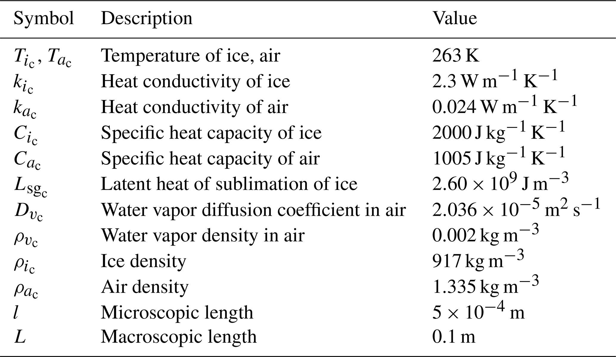
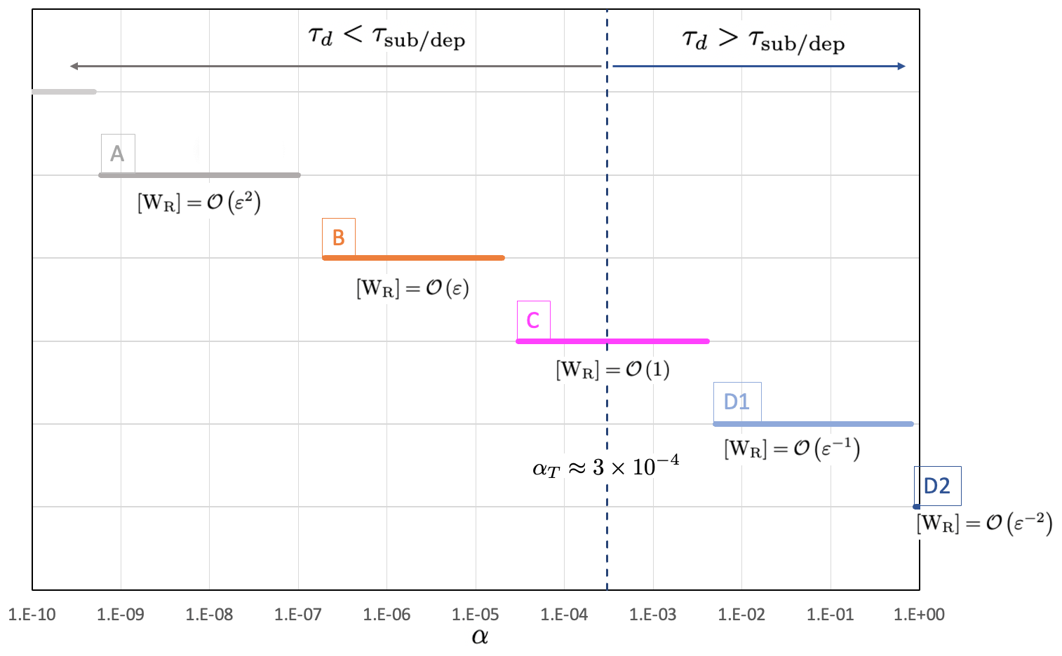
Figure 2Estimation of the dimensionless number [WR] with respect to α, which leads to several cases of macroscopic modeling to be considered (cases A to D2). The αT value characterizes the transition between two cases presenting different limiting processes for the water vapor transfer at the pore scale, so that or , with τd as the characteristic time associated with water vapor diffusion and as the characteristic time associated with the sublimation–deposition process. αT was estimated based on the characteristic values given in Table 1.
Estimations of the dimensionless number [H] are not as straightforward, as they depend on the intensity of the interface normal growth velocity . When αc is small (typically smaller than αT), [WR] is also small, and Eq. (18) implies that has a finite value (𝒪(ρvc)). Thus, this dimensionless number [H] can be also written as
In that case, it increases when αc increases, and according to the characteristic values given in Table 1, it is of the same order as [WR]. For large values of αc (typically larger than αT), Eq. (18) implies that . As a consequence, from Eqs. (17) and (19), [H] can be rewritten as
where is the derivative of the Clausius–Clapeyron law, and can be seen as an enhancement of the air thermal conductivity. Using the characteristic values given in Table 1 and the Clausius–Clapeyron equation, Eq. (9), for large values of αc, [H]=𝒪(1). According to the above analysis, several cases must be considered, depending on the value of the condensation coefficient αc (Fig. 2).
-
Case A is , i.e., [WR]=𝒪(ε2) and [H]=𝒪(ε2).
-
Case B is , i.e., [WR]=𝒪(ε) and [H]=𝒪(ε).
-
Case C is , i.e., [WR]=𝒪(1) and [H]=𝒪(1).
-
Case D1 is , i.e., and [H]=𝒪(1).
-
Case D2 is , i.e., and [H]=𝒪(1).
Cases A and B correspond to , whereas cases D1 and D2 correspond to . Case C ensures the transition between cases B and D1, when α≈αT.
2.5 Asymptotic analysis
The next step is to introduce multiple-scale coordinates (Bensoussan et al., 1978; Sanchez-Palencia, 1980; Auriault, 1991). The two characteristic lengths L and l introduce two dimensionless space variables, and , where X is the physical space variable. The macroscopic (or slow) dimensionless space variable x* is related to the microscopic (or fast) dimensionless space variable y* by . When l is used as the characteristic length, the dimensionless derivative operator grad* becomes (, where the subscripts and denote the derivatives with respect to the variables x* and y*, respectively. Following the multiple-scale expansion technique (Bensoussan et al., 1978; Sanchez-Palencia, 1980; Auriault, 1991), the ice temperature , the air temperature , and the water vapor are sought in the form of the asymptotic expansion of the powers of ε, as follows:
where , and the corresponding φ*(i) are periodic functions of period Ω with respect to the space variable y*. Substituting these expansions in the set (13)–(18) gives, through the identification of identical powers of ε, successive boundary value problems to be investigated. All the details concerning this asymptotic analysis are presented in the Supplement. The main results are summarized in the following section.
2.6 Macroscopic-equivalent descriptions
2.6.1 Case A
Case A corresponds to the model presented in Calonne et al. (2014b). According to the order of magnitude of the dimensionless numbers, and notably , the asymptotic analysis presented in the Supplement (Sect. S1) shows that the heat transfer and the water vapor diffusion at the macroscopic scale are described by Eqs. (S.A.44) and (S.A.47). Returning dimensional variables, the macroscopic model is written as
where is given by the Hertz–Knudsen equation (Eq. S.A.43) and the Clausius–Clapeyron law (Eq. S.A.42; see Sect. S1 in the Supplement),
and where ϕ is the porosity and its total time derivative. is the specific surface area per unit volume, defined as the ice surface area over the snow volume (in m−1). The SSA can also be defined per unit mass, with . (ρC)eff is the effective thermal capacity (Eq. S.A.45), keff is the effective thermal conductivity tensor (Eq. S.A.46), and Deff is the effective diffusion tensor (Eq. S.A.48). These effective properties are defined as
where ta and ti are two periodic vectors. The solution of the following boundary value problem over the REV Eqs. (S.A.20)–(S.A.24) is as follows:
Moreover, gv is a periodic vector solution of the following boundary value problem over the REV Eqs. (S.A.35)–(S.A.37):
In that case, the above macroscopic equivalent description shows that, at the first order, the heat and water vapor transfer are described by two equations which are coupled through a source term proportional to the Hertz–Knudsen equation (Eq. 23) and the Clausius–Clapeyron law (Eq. 24) but expressed with respect to the two macroscopic variables T(0) and . These equations involve two effective parameters, namely the effective thermal conductivity and the effective diffusion .
2.6.2 Case B
According to the order of magnitude of the dimensionless numbers in case B, the asymptotic analysis presented in the Supplement (Sect. S2) shows that the heat transfer and the water vapor diffusion at the macroscopic scale are described by Eqs. (S.B.29) and (S.B.44). Returning dimensional variables, the macroscopic model is written as
with
where (ρC)eff is the effective thermal capacity, keff is the effective thermal conductivity tensor, and Deff is the effective diffusion tensor, as defined in case A. The above macroscopic equivalent description shows that, at the first order, the heat and vapor transfer are only driven by the temperature field, since the water vapor density is directly given by the Clausius–Clapeyron law (Eq. 24). Consequently, from Eq. (37), we have the following:
where
Taking this result into account, the macroscopic heat transfer equation (Eq. 36) is written as
In this latter equation,
which appears as an apparent thermal conductivity of the snow which depends non-linearly on the temperature through γ(T(0)). Our results show that this is valid if [WR]=𝒪(ε), i.e., typically for α values ranging from around 2 × 10⁻⁷ to 2 × 10⁻⁵. Finally, let us remark that (i) model B can be also seen as a particular case of model A when tends towards by increasing α, and (ii) the apparent thermal conductivity of the snow can also be written as
where corresponds to an enhancement of the air thermal conductivity, as defined in Sect. 2.4. However, in that case, γ(T(0)) depends on the macroscopic temperature T(0).
2.6.3 Case C
According to the order of magnitude of the dimensionless numbers in case C, the asymptotic analysis presented in the Supplement (Sect. S3) shows that the heat transfer and the water vapor diffusion at the macroscopic scale are described by Eqs. (S.C.42) and (S.C.47). Returning dimensional variables, the macroscopic model is written as
with
where (ρC)eff and kC are the dimensionless effective thermal capacity and the effective dimensionless thermal conductivity, respectively, and defined as
where DC is the effective diffusion tensor defined as
Moreover, si, sa, and d are the periodic vector solutions of the following coupled boundary value problem in a compact form (see Sect. S3 and Eqs. S.C.30–S.C.37 in the Supplement):
with
The vectors si, sa, and d depend on the values of α and the temperature (notably through γ(T(0))). As for model B, the macroscopic heat transfer equation (Eq. 44) can also be written as
where
which appears as an apparent thermal conductivity of the snow. In that case kC and DC both depend on ka, ki, kdif, and α, and we have
This model C is valid for [WR]=𝒪(1), i.e., for and thus for α values in the range or, typically, .
2.6.4 Cases D1 and D2
According to the order of magnitude of the dimensionless numbers in cases D1 and D2, the asymptotic analysis presented in the Supplement (Sect. S4) shows that these two cases lead to the same macroscopic description. Returning dimensional variables, the macroscopic model (Eqs. S.D1.41–S.D1.45 or Eqs. S.D2.41–S.D2.45) is written as
(ρC)eff is the classical dimensionless effective thermal capacity. The macroscopic thermal conductivity tensor kD and the macroscopic diffusion tensor DD are defined as
where ra and ri are two periodic vectors. The solution of the boundary value problem over the REV Eqs. (S.D1.30)–(S.D1.34) is as follows:
As for models B and C, the macroscopic heat transfer equation (Eq. 61) can be also written as
In this latter equation,
which appears as an apparent thermal conductivity of the snow. In that case, kD and DD both depend on ka, ki, and kdif, and we have
This model D corresponds to the one derived by Moyne et al. (1988), assuming that ρv=ρvs(T) is on the interface at the microscopic scale and using the volume averaging method. This model is also similar to the one derived by Hansen and Foslien (2015), assuming that . In that case, we show that this model is valid for or 𝒪(ε−2), i.e., typically for α values ranging from around 5 × 10⁻³ to 1.
2.7 Macroscopic equivalent descriptions – synthesis
Figure 3 presents a summary of the four macroscopic models of heat and vapor transport in dry snow derived above, together with their domain of validity according to the value of α. As already mentioned, model A is the one already derived in Calonne et al. (2014b), whereas model D is equivalent to the model derived by Moyne et al. (1988) and Hansen and Foslien (2015).
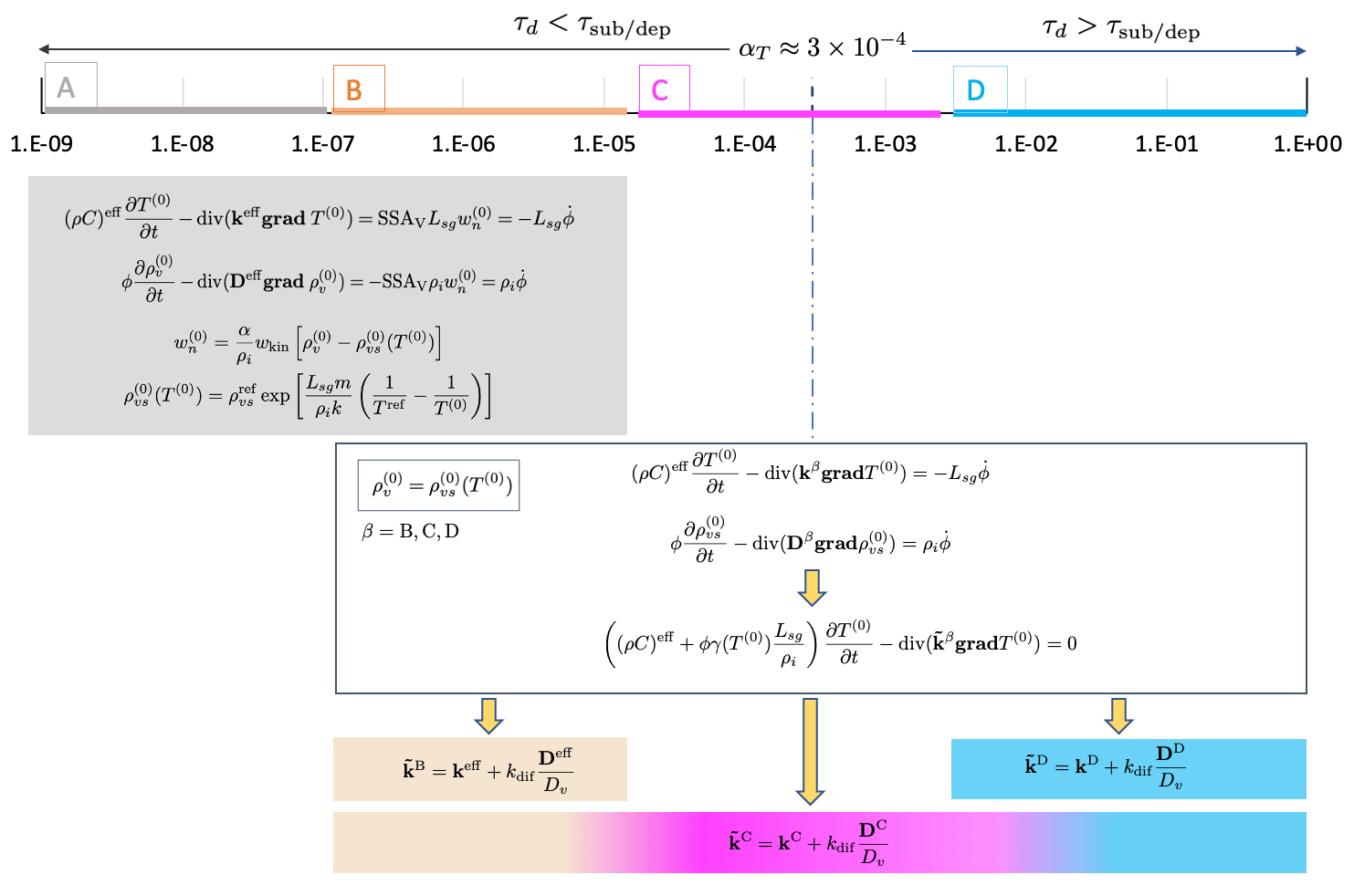
Figure 3Definition of the three different macroscopic models and their domain of validity with respect to α. The value of αT was estimated based on the characteristic values given in Table 1.
A first important outcome is that the hypothesis ρv=ρvs(T), which is often made, appears to be a good approximation for α values larger than 10−6, as seen for models B, C, and D. The asymptotic analysis shows that in the range of α [10−6, αT], this approximation is of the order of 𝒪(ε) since , i.e., . In the range [αT, 1], this approximation is of the order of 𝒪(ε2), since and , i.e., σ≈𝒪(ε2). This result implies that models B, C, and D can be written in the same form and be reduced to a simple heat transfer equation. This heat transfer equation involves an apparent thermal conductivity , which differs from one model to another. In contrast, model A does not presume any assumption about the vapor saturation.
A second point concerns the relative role of the vapor diffusion and of the sublimation–condensation in the vapor transport, which directly impacts the model formulation. In models A and B, the water vapor transfer is mainly limited by the sublimation–deposition at the ice–air interfaces. Model A consists of two equations of temperature and vapor density coupled through source terms that are proportional to α. Classically, heat and vapor transport are driven by the effective thermal conductivity of snow keff and the effective vapor diffusivity of snow Deff, respectively. Both properties depend on the intrinsic properties of ice and air (ki,ka, and Dv) and on the snow microstructure. Model B can be seen as a particular case of model A, assuming that ρv tends towards ρvs(T) at the macro-scale, leading to a simplification in the form of one heat transfer equation in which the apparent thermal conductivity can be easily expressed with respect to keff (ki, ka, and microstructure) and Deff (Dv, and microstructure).
In contrast, in model D, the water vapor transfer is mainly limited by the diffusion process at the micro-scale. In that case, the model consists of a single heat transfer equation in which α is not involved but instead driven by an apparent thermal conductivity , which can be expressed with respect to the macroscopic thermal conductivity kD (ki, ka, kdif, and microstructure) and to the macroscopic diffusion DD (Dv, ki, ka, kdif, and microstructure), with the latter appearing as a thermodiffusion coefficient. Note that these parameters depend on the air thermal properties ka+kdif that are enhanced by the phase change through kdif.
The transition between a diffusion-limited and sublimation–deposition-limited vapor transport is captured by model C. This transition appears around a transition value αT estimated here at , yet we recall that it can vary between 10−5 and 10−3, depending on the grain size and, to a lesser extent, on temperature. Model C is of the same form as models B and D, but the apparent thermal conductivity can be expressed with respect to the macroscopic thermal conductivity kC (ki, ka, kdif, α, and microstructure) and the macroscopic diffusion DC (Dv, ki, ka, kdif, α, and microstructure). Unlike the other models, both macroscopic parameters kC and DC depend on α. These parameters tend towards keff and Deff when α tends towards 10−5, thus recovering model B. They also tend towards kD and DD when α tends towards 1, thus recovering model D. Consequently, in practice, models A and C are sufficient to describe the heat and vapor transfer in the whole range of α (see Sect. 3.3).
In this section, two simple snow microstructures, a bilayer snowpack and an assemblage of spherical grains and pores, are first considered to illustrate the influence of the microstructure and of the parameters taken at the pore scale on the macroscopic parameters of models A, B, and D (Sect. 3.2 and 3.1).
Then, a simplified 2D snow microstructure is considered to evaluate the models by comparing simulation results obtained with the pore-scale description and with the macroscopic modeling (Sect. 3.3).
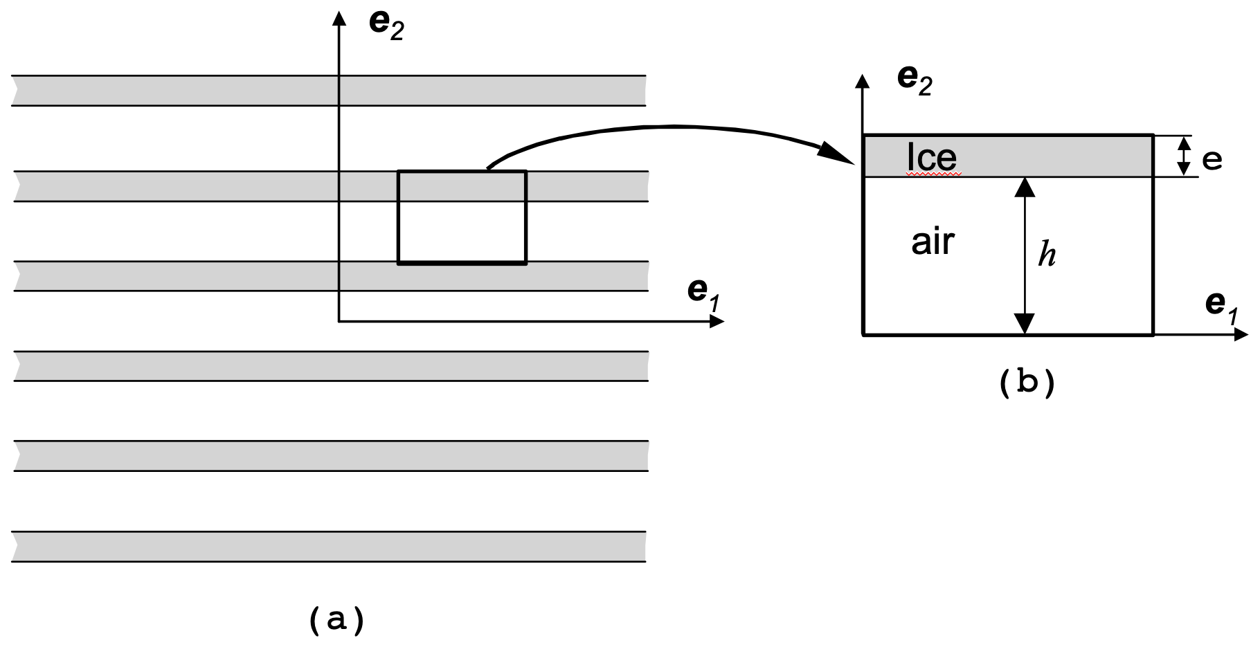
Figure 4Illustration of the bilayer snowpack problem (a) at the macroscopic scale and (b) at the scale of a representative elementary volume (REV).
3.1 The bilayer snowpack: upper and lower bounds
As a first example, we consider the classical bilayer material problem, and the snowpack is seen as a succession of horizontal layers of pure air and of pure ice, as illustrated in Fig. 4. In this case, the macroscopic parameters arising in models A, B, and D can be analytically determined and constitute the upper and lower bounds of these parameters for any anisotropic snow microstructure. The boundary value problems in (Eqs. 33–35), (28–32), and (66–70) have been solved analytically on the REV (Fig. 4b) in Auriault et al. (2009). Taking into account those results and using Eqs. (27) and (26), we have, for models A and B,
Thus, it follows that
These results imply that the macroscopic properties (Deff,keff, and ) of any anisotropic snow verify the following bounds:
and
For model D, from Eqs. (65) and (64), we have
Thus, it follows that
In that case, these results imply that the macroscopic properties (DD,kD, and ) of any anisotropic snow verify the following bounds:
and
The above results show that, as already emphasized in Calonne et al. (2014b), Moyne et al. (1988), and Fourteau et al. (2021b), the bounds in Eqs. (77) and (82) of both the effective diffusion coefficients Deff and DD are always smaller than Dv and DD>Deff, whatsoever the α value. Moreover, according to the definition of Deff (Eq. 74) and DD (Eq. 79), if a vertical macroscopic temperature gradient is applied along e2, model A (or B) will not predict any porosity variation along that direction because of the pore geometry. By contrast, model D, where the sublimation–deposition process is faster than diffusion, can predict mass transport along e2, since , and thus a variation in the porosity along e2.
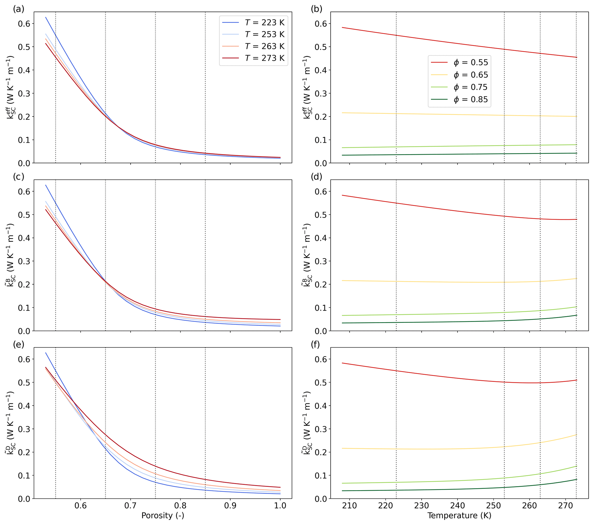
Figure 5Evolution of the SC estimates of the thermal conductivities , , and with respect to porosity at four temperatures (a, c, e) and with respect to temperature for four porosities (b, d, f). The vertical dotted gray lines indicate the four temperature and porosity values considered.
3.2 Assemblage of spherical grains and pores: self-consistent estimates
The next analytical model is the self-consistent model (Bruggeman, 1935; Hill, 1965; Budiansky, 1965; Torquato, 2002). Previous works showed that self-consistent (SC) estimates provide good estimations of the macroscopic properties of heat and vapor transport in dry snow (Calonne et al., 2014b, a, 2019). In this model, the snow microstructure is considered a macroscopically isotropic material made of an assemblage of spherical inclusions of air or ice. Each type of inclusion is embedded in a homogeneous equivalent material, allowing us to account for the connectivity of both phases. The equivalent material corresponds to an infinite matrix for which the effective properties are the unknown to be calculated. The solution of the equations for an isolated inclusion then gives an implicit relation which can be solved for this effective property.
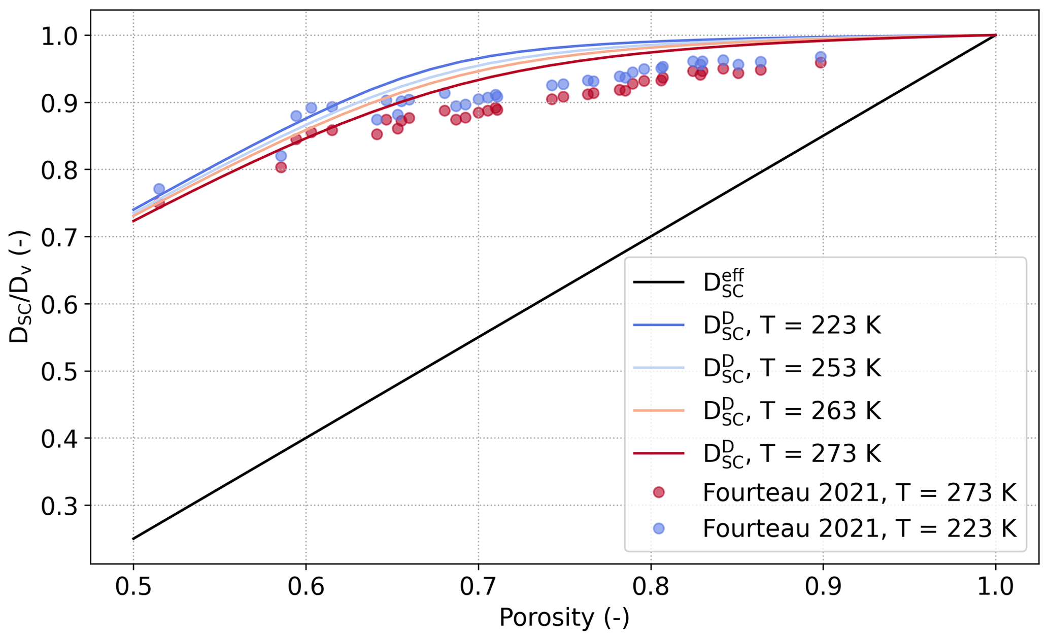
Figure 6Evolution of the normalized SC estimates and with respect to porosity at different temperatures (solid lines). Results of the numerical computations of at two temperatures from Fourteau et al. (2021a) are also shown (symbols).
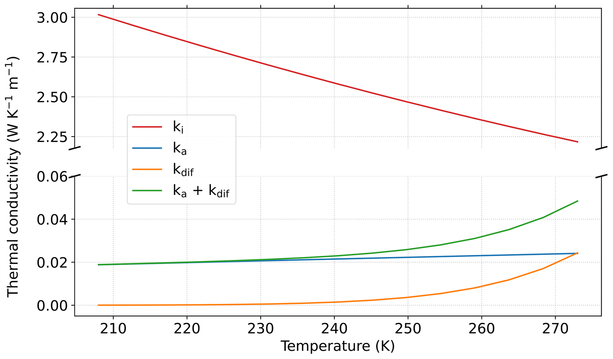
Figure 7Evolution of the thermal conductivity with temperature for ki (Huang et al., 2013), ka (Haynes, 2016), kdif, and ka+kdif.
For model A, the SC estimate of the effective thermal conductivity of snow and of the effective diffusion coefficient verify the following implicit relation (Torquato, 2002):
For model B, the SC estimate of the thermal conductivity is obtained by replacing the effective properties by their SC estimates in Eq. (41) and reads
Finally, for model D, the SC estimate of thermal conductivity can be obtained by replacing ka in Eq. (84) with ka+kdif as follows:
For the diffusion coefficient , it can be shown that (Auriault et al., 2009)
The above SC estimates of the thermal conductivity and diffusion coefficient are presented in Figs. 5 and 6, and the impact of snow porosity and temperature is shown. To do so, we used the relationships of the thermal conductivity of ice ki(T) and of air ka(T), with the temperature from Huang et al. (2013) and Haynes (2016), respectively.
For thermal conductivity, the SC estimates , , and at a given temperature are similar and follow the classical exponential evolution with snow porosity. Overall, estimates vary between about 0.06 W m−1 K−1 for porosity of 0.5 and 0.01 W m−1 K−1 for porosity of 1 (Fig. 5a, c, and e). More differences between the estimates can be seen for the normalized diffusion coefficient. The effective coefficient is overall much smaller than and evolves linearly from 0.25 to 1 when porosity varies from 0.5 to 1 (Fig. 6). In contrast, shows a non-linear evolution from 0.7 to 1, with values close to 1 for porosity above 0.8. The non-linearity and the high values of come from the contribution of the heat conduction, through , and of the latent heat, through kdif. Finally, those estimates are in good agreement with the computed values from 3D images of snow in Fourteau et al. (2021a).
Next, we look at the impact of temperature on the properties. The impact is weaker than the one of porosity and more complex to understand, as dependencies are multiple. To help understand, we first break down the dependencies and show in Fig. 7 how the variables kdif and ka+kdif and the thermal conductivity of ice ki and air ka evolve with temperature. When temperature increases from 210 to 273 K, the thermal conductivity of ice decreases, and the one of air slightly increase, with both evolutions being quasi-linear. Non-linearity is introduced with the parameter kdif, which increases exponentially with temperature. Values for this parameter are small, even smaller than the air thermal conductivity, and are close to 0 W m−1 K−1 at −60 °C and reach 0.02 W m−1 K−1 at −3 °C. Finally, the term ka+kdif evolves in the same way as kdif (non-linear), but the values are increased by ka.
Keeping the above considerations in mind, the evolution of , , and with temperature is presented in Fig. 5b, d, and f. For , the SC estimates basically follow a monotonous decrease in the thermal conductivity with increasing temperature. This decrease is less pronounced for high porosity, and vice versa. These features directly result from the impact of the evolution of the ice and air thermal conductivity with temperature. The evolution of and with temperature is more complex as the impact of kdif superimposes. They show a non-linear evolution with temperature, with an evolution similar to for the lower temperatures and transitioning to an exponential increase for the higher temperatures, where the latter is driven by kdif. We see that this non-linearity is even more important for than for , as kdif appears in the definition of several times. Finally, estimates of diffusion coefficient show a slight influence of temperature through ki, ka, and kdif and increase with decreasing temperature, in agreement with Fourteau et al. (2021a).
3.3 Numerical evaluation on a simplified 2D geometry
We perform a numerical evaluation of the obtained macroscopic models on a simplified 2D snow microstructure, as in Calonne et al. (2014b). We compare simulations of heat and water vapor transfer in snow obtained with the pore-scale description and with the macroscopic modeling.
3.3.1 Case study definition
Finite element numerical simulations were performed using the code from COMSOL Multiphysics software on a 2D vertical snow layer of 10 cm height and 0.5 cm width (Fig. 8). A constant temperature gradient of 100 or 500 K m−1 was applied across the layer. Temperatures at the top Ttop and at the bottom Tbottom are imposed, and Tbottom is kept at 273 K. For the water vapor conditions at the top and bottom, a null vapor flux is applied. Symmetry conditions are imposed on the lateral sides of the snow layer. Simulations were run in a steady state.
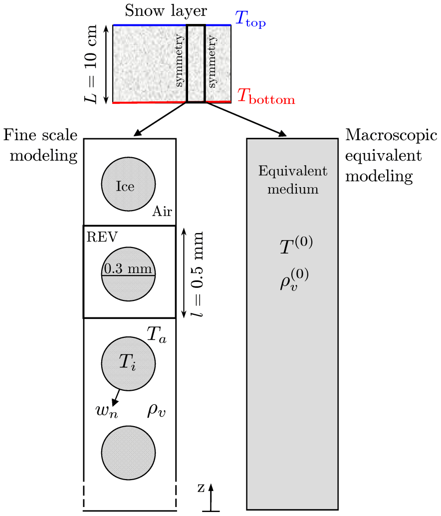
Figure 8Illustration of the 2D geometry for the pore-scale modeling and the macroscopic equivalent modeling.
At the pore scale, the snow layer consists of 200 periodic cells of 0.5 × 0.5 mm2; each periodic cell (REV) is composed of an ice grain with a diameter of 0.3 mm surrounded by air, as shown in Fig. 8. The snow porosity is 0.71, which corresponds to a density of 266 kg m−3. The heat and the mass transfer is described by the set of Eqs. (1)–(12), where Ti, Ta, and ρv are the unknowns. This set of equations was numerically solved using the material parameter values presented in Table 1 and for different α values in the range of 10−10 to 1. For the sake of simplicity, the thermal conductivities ki and ka were kept constant in all the simulations. The chosen values correspond to a temperature of −10 °C (Table 1).
At the macroscopic scale, the snow layer is seen as a continuous equivalent medium. The heat and the mass transfer is described by the homogenized equations Eqs. (21)–(23) for model A, Eqs. (41) and (37) for model B, Eqs. (58) and (45) for model C, and Eqs. (71) and (62) for model D, where T(0) and are the macroscopic unknowns. These macroscopic descriptions involve different parameters and properties defined over the REV, which need to be provided. The porosity and the specific surface area SSAV were equal to 0.71 and 3770 m−1, respectively. The effective properties keff and Deff were computed over the REV composed of a unique cell by solving the boundary value problems in Eqs. (33)–(35) and Eqs. (28)–(32), respectively. Given the symmetry of the REV, all the tensors involved in the macroscopic descriptions are isotropic. We found that keff=0.04243 W m−1 K−1 and m2 s−1. The apparent thermal conductivity was analytically deduced using Eq. (41). Its value depends on the temperature through the term kdif(T). and DC were computed over the REV by solving the boundary value problem in Eqs. (50)–(57) at different temperatures by varying the term ka+kdif(T) for α values in the range 10−6 to 1. Finally, and DD were computed over the REV by solving the boundary value problem in Eqs. (66)–(70) at different temperatures in a similar way. In the considered temperature range, DD is almost constant and equal to m2 s−1.
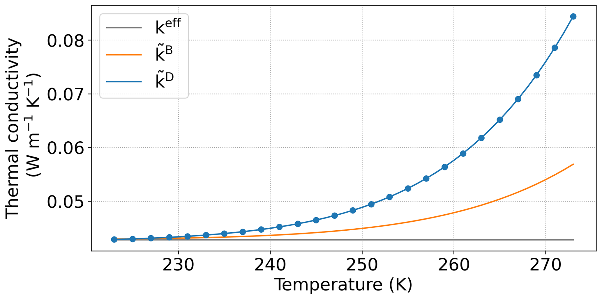
Figure 9Evolution of the thermal conductivities keff, , and with temperature. For , the blue dots represent the numerical estimates over the REV, and the blue line is the fit.
Figure 9 presents the evolution of keff, , and with temperature. As expected, and evolve non-linearly with T. To perform the simulations, the computed values of were fitted by the following relation: (blue line in Fig. 9). Figure 10 shows the evolution of the dimensionless diffusion coefficients , , and and of the macroscopic thermal conductivities keff, kC, and kD with respect to α and for two temperatures of 270 and 250 K. As expected, only the parameters of model C ( and kC) vary with α and ensure a continuous transition between the parameters of model A ( and keff) and the ones of model D ( and kD). When fitting the numerical estimates, such a transition can be described by a simple function as follows:
where A=1200 is a constant. This fit is shown with black lines in Fig. 10. The figure also includes the numerical estimations of the diffusion coefficient on 3D snow microstructures of different densities from Fourteau et al. (2021b), which are in good agreement with the proposed function in Eq. (89).
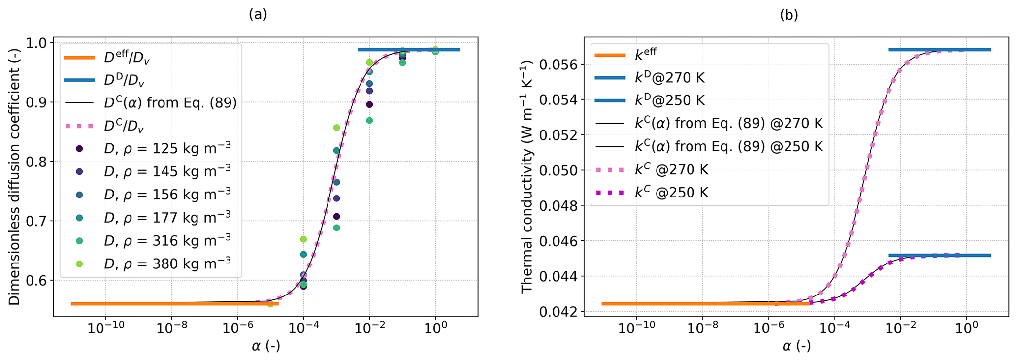
Figure 10Evolution of the dimensionless diffusion coefficients , , and and of the macroscopic thermal conductivities keff, kC, and kD with respect to α and for two temperatures (270 and 250 K). The black lines represent the proposed function in Eq. (89) to describe the parameters of model C. Numerical estimates of the diffusion coefficient on 3D snow microstructures of different densities from Fourteau et al. (2021b) are represented by the dots.
3.3.2 Comparison between pore-scale and macro-scale simulations
Results between pore-scale and macro-scale simulations are compared in terms of temperature, vapor density, and mass change rate. At the pore scale, the average values of each variable were taken over the cell and computed as follows:
Thus, we compare the vertical profiles of the pore-scale variables 〈T〉, 〈ρv〉, 〈ρvs〉, and with the vertical profiles of the macroscopic variables T(0), , , and . As the obtained simulated temperature profiles were close to each other, to ease the comparison, we also use the temperature deviation ΔT, which represents the deviation of the simulated temperature profile from the linear temperature profile imposed by Ttop and Tbottom, as illustrated in Fig. 11. In the same vein, we use the water vapor supersaturation, which is the difference between the simulated water vapor density and the saturated water vapor density ρv−ρvs(T). Figure 12 shows the vertical profiles of ΔT, of ρv−ρvs(T), and of from the pore-scale simulations (dots) and the macroscopic models (lines), considering a temperature gradient of 100 and 500 K m−1. For the pore-scale simulations, values of α from 10−9 to 1 were used. For the macroscopic models, results are only shown in their domain of validity with respect to α. To further highlight the impact of α, Fig. 13 presents the evolution of T, ρ, and ρvs with α for the specific middle cell of the snow layer, which is here the 100th cell from the bottom ( and ). Again, pore-scale simulations (dots) and the macroscopic models (line) are compared.
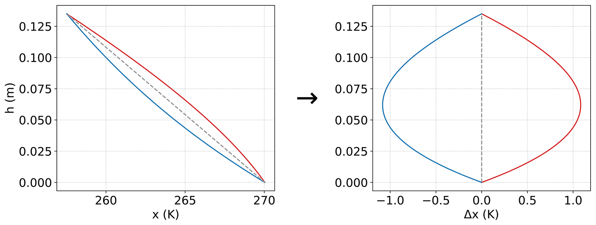
Figure 11Simplified example of the transition from the x to Δx notation in a concave (red) and a convex (blue) case.
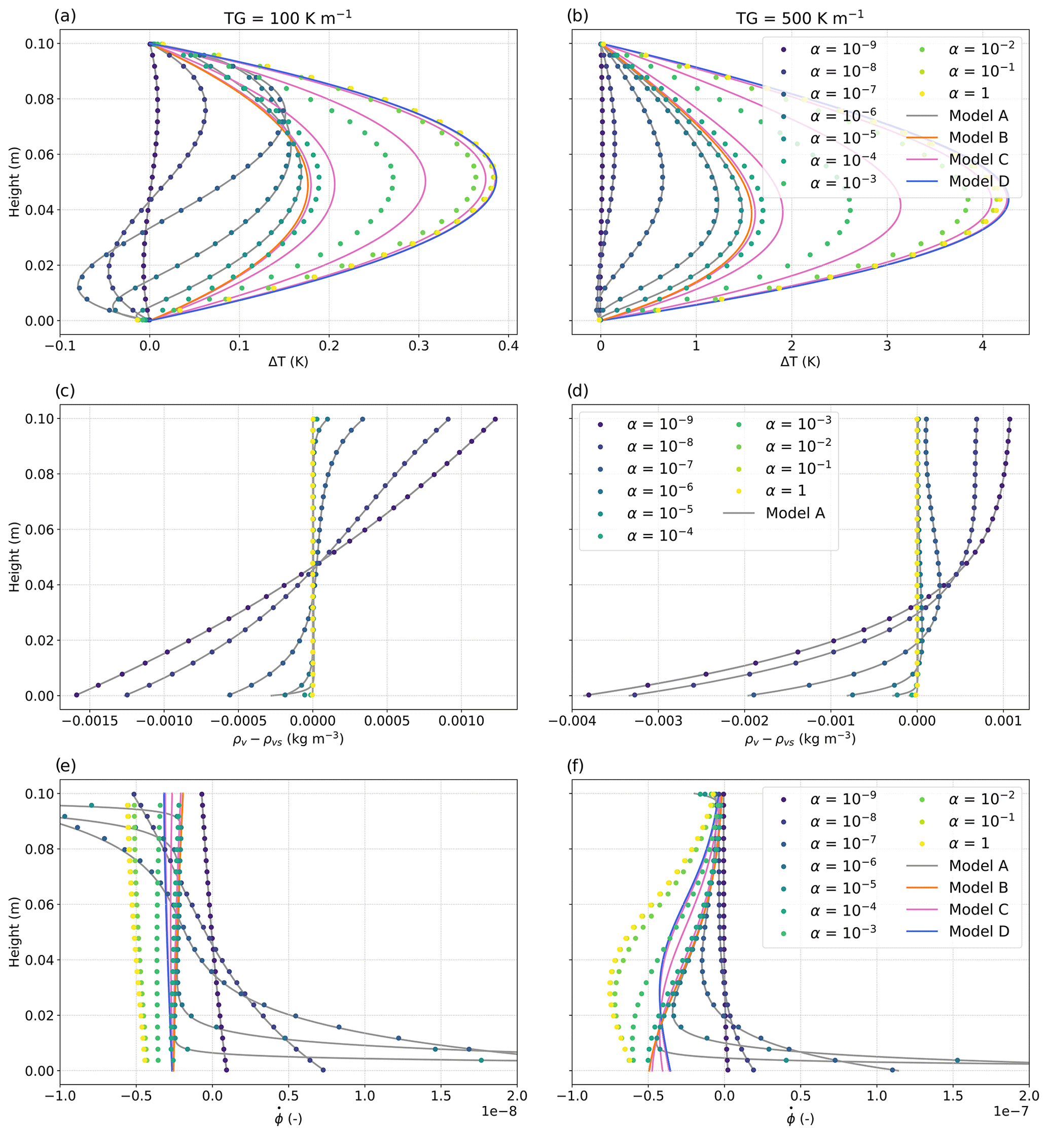
Figure 12Vertical profiles of ΔT, ρv−ρvs(T), and from the pore-scale simulations (dots) and from the macroscopic models A (grey lines), B (orange lines), C (magenta lines), and D (blue lines), considering a temperature gradient of 100 and 500 K m−1 and for different values of α. ΔT represents the deviation of the temperature profile from a linear temperature profile. Predictions of ρv−ρvs(T) from models C and D are not shown in panels (c) and (d), as they are superimposed with the pore-scale simulation results for α = 1 (dotted yellow lines).
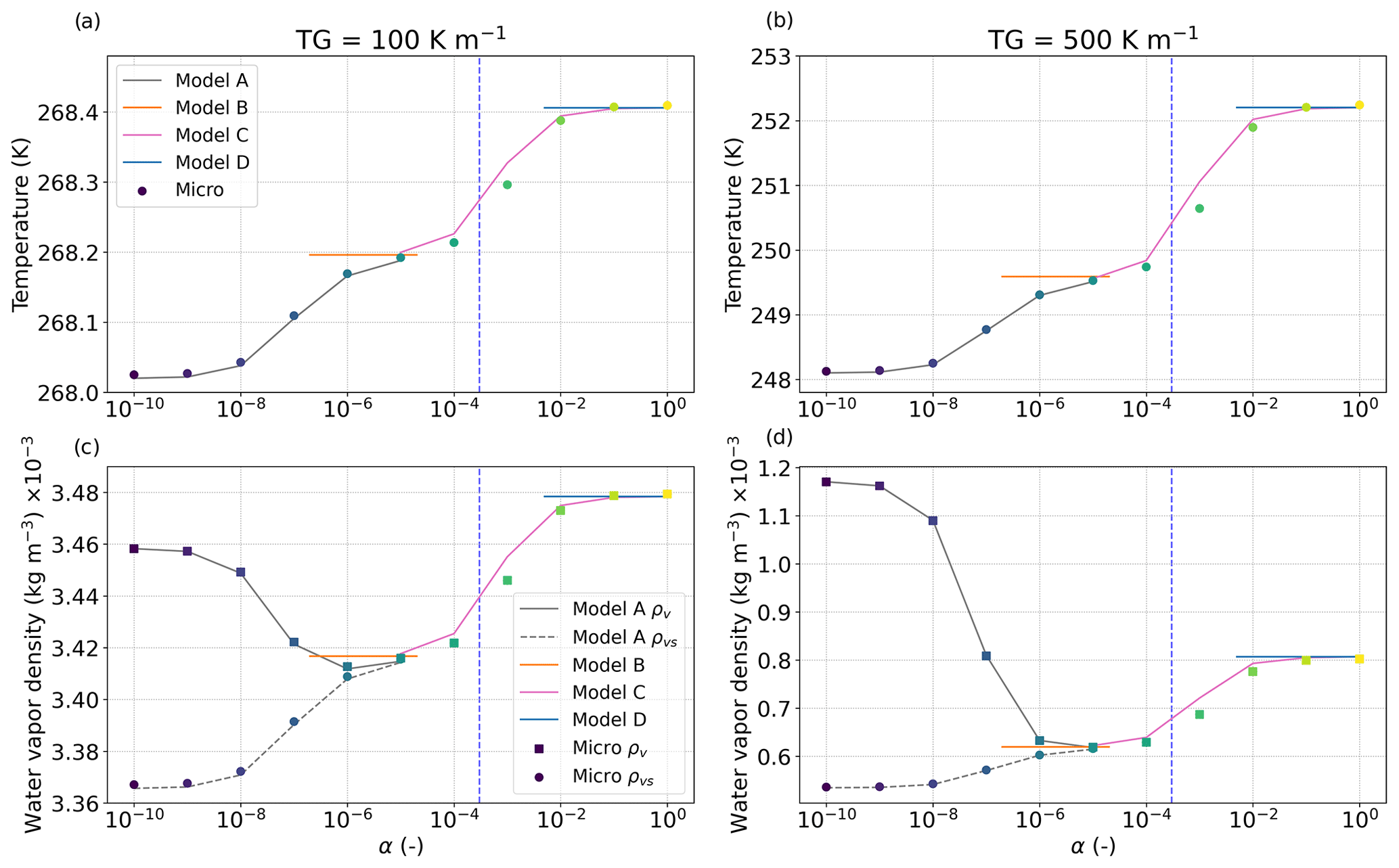
Figure 13Temperature and water vapor density in the middle of the snow layer as a function of α, obtained from the pore-scale simulations (dots) and from the macroscopic models A (grey lines), B (orange lines), C (magenta lines), and D (blue lines) at 100 and 500 K m−1. The models are only shown for the α values within their domain of validity. Values of saturation water vapor density ρvs from the pore-scale simulations and from model A are also presented.
We describe first the main features observed in the pore-scale simulations. All the variables show an impact of the α value. The temperature deviation ΔT is overall mainly positive (Fig. 12a and b), which reflects the presence of a heat source by non-conductive processes such as latent heat from deposition. This temperature deviation increases with α and with the temperature gradient. This is also reflected in the temperature of the middle cell that overall increases with increasing α (Fig. 13a and b). This increase is not uniform, and two plateaus are observed – one between and the other one between . The largest ΔT value is reached in the center of the snow layer and is around 0.4 K at 100 K m−1 and 4 K at 500 K m−1. Looking at the lower part of the layer, negative ΔT values can be found for and indicate a heat loss by non-conductive processes such as latent heat from sublimation. This feature vanishes for the large temperature gradient. In terms of water vapor supersaturation ρv−ρvs(T), we observe positive values (over-saturation) in the upper part of the snow layer, values close to zero in the central part (at saturation), and negative values (under-saturation) in the lower part (Fig. 12c, d). The largest over-saturation and under-saturation values are shown for low α values when phase changes are very limited. With increasing α values, values close to saturation get predominant, and the over-saturation and under-saturation zones become localized near the top and bottom, respectively. This is confirmed in Fig. 13c and d, where ρv≈ρvs(T) for . Similar to the temperature, two plateaus are shown where ρv−ρvs(T) evolve little with α. All of these results are consistent with our theoretical analysis presented in Sect. 2. Last, the vertical profiles of are consistent with the ones of supersaturation, showing deposition in the upper part where the porosity decreases and sublimation in the lower part where the porosity increases (Fig. 12e and f). As α increases, those transitions become sharper and sharper, like a front. For , most values become negative, indicating overall deposition in the snow layer. A sublimation zone is still visible at the bottom of the snow layer, but its thickness is typically of the order of a few REV or smaller. Finally, as the difference ρv−ρvs is directly related to the interface growth velocity wn (see Eq. 10), and as it could be useful to compare it with experimental estimates (e.g., Flin and Brzoska, 2008; Brzoska et al., 2008; Pinzer et al., 2012; Libbrecht and Rickerby, 2013), we provide below the mean values of wn computed for the bottom and middle cell of α = 10−6. For 100 K m−1, a value of 5.9 × 10⁻¹³ m s−1 and of −2.7 × 10⁻¹¹ m s−1 is found in the middle and bottom cell, respectively. For 500 K m−1, a value of 4.5 × 10⁻¹² m s−1 and of −1.1 × 10⁻¹⁰ m s−1 is found in the middle and bottom cell, respectively.
Next we compare the different macroscopic models to the pore-scale simulations. In both Figs. 12 and Fig. 13, the comparison shows different behaviors, depending on α. For , model A reproduces precisely all the features shown at the pore scale. Models B and D are independent of α and provide one estimate of the temperature, and thus the water vapor density, for all the α values in their domain of validity. These estimates are only able to reproduce the plateau values observed in the pore-scale simulations, i.e., temperatures for for model B and for model D (Fig. 13). Model C, which depends on α, allows us to reproduce the main features shown at the pore scale for α values in the range . This model predicts ΔT values higher than the pore-scale simulations for a given α. Moreover, models B, C, and D predict only the deposition in snow, with negative values throughout the layer (Fig. 12e and f). They do not capture the sublimation front at the bottom of the snow layer, in contrast to model A. The mass balance between sublimation–deposition over the whole snow layer is not well satisfied; the Dirichlet boundary condition imposed on the temperature field at the bottom and the top of the snow cannot ensure that the water vapor flux is null at the same time since ρv=ρvs(T). This limitation can explain the slight differences that we can observe between model C predictions and the pore-scale simulations. In order to overcome this limit, specific boundary conditions should be introduced to allow the description of mass variations near the interfaces.
This section presents the evaluation of the macroscopic models A, B, and D, based on observations of natural snow evolution from three cold-laboratory TGM experiments. We first introduce the experimental data (Sect. 4.1); then we define the estimates to be taken for the input parameters of the models (Sect. 4.2); and, finally, we present the simulation results with the models and their comparison with the experiments (Sect. 4.3).
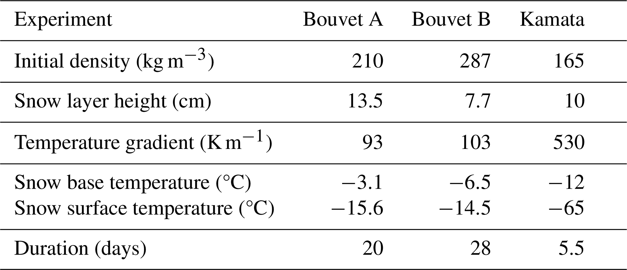
Table 2Overview of the experimental settings used in the simulations.
4.1 Experimental datasets
We used the datasets provided by Bouvet et al. (2023), consisting of two experiments, referred to as Bouvet A and Bouvet B in their paper and hereafter, and the data from Kamata and Sato (2007), referred to as Kamata. These experiments provide the required data to evaluate our models, namely the time series of the vertical profiles of temperature and density of a snow layer evolving under a temperature gradient in a controlled environment. The main characteristics of the three experiments are summarized in Table 2. Bouvet A is a TGM experiment on a 13.5 cm high snow layer for which a temperature gradient (TG) of 93 K m−1 was applied during 20 d. X-ray tomography was done at regular time intervals resulting in 9 large 3D images of the whole vertical dimension of the snow layer at a resolution of 21 µm and 17 small 3D images of the top or bottom part of the layer at a resolution of 8 µm. For the large images, the first few millimeters at the base of the layer are lacking, due to the snow sampling procedure, so no data are available for this area. This experiment also includes monitoring of the temperature profile of the snow layer, measured using seven Pt100 sensors. Bouvet B is a TGM experiment on a 7.7 cm high snow layer for which a TG of 103 K m−1 was applied during 28 d. Four tomography images of the first lower 4.2 cm of the snow layer are provided at a resolution of 10 µm. For both experiments, Bouvet A and Bouvet B, the vertical profiles of the snow density computed from the 3D images are provided, and a vertical mass redistribution can be analyzed. Finally, the Kamata experiment is a TGM experiment on a snow layer of 10 cm height for which an extreme TG of 530 K m−1 was applied during 5.5 d (133 h). The vertical mass redistribution was estimated by measuring snow density for four sections of the snow layer. For that, the snow layer was separated into vertical compartments of about 2.5 cm height each, using horizontal nylon meshes, which enables water vapor to get through. Each compartment was weighed at the initial and final stage of the experiment. In addition, the temperature was recorded at six vertical locations.
4.2 Effective properties and parameters
Next we study the estimates of the effective properties and other input parameters required to run models A, B, and D. For the sake of simplicity, model C is not systematically shown. For each model, these properties are computed from the 3D images of snow of the experiment Bouvet A and Bouvet B. Those values are then compared to different parameterizations from the literature or fitted regressions, and we select the more suited ones to be used later in the models.
4.2.1 Model A
Model A involves three effective parameters that are the effective thermal conductivity keff, the effective vapor diffusivity Deff, and the SSA (Sect. 2.6.1). These parameters were estimated in the case of Bouvet A and Bouvet B by numerical computations on the 3D tomographic images available. The SSA was computed per unit of mass based on the voxel projection approach (Flin et al., 2011; Dumont et al., 2021). keff and Deff were computed with the GeoDict software (Thoemen et al., 2008) by solving the boundary value problems in Eqs. (28)–(32) and Eqs. (33)–(35) on the 3D images and by applying periodic boundary conditions on the external boundaries, as described in Calonne et al. (2011, 2014b). Values of ki and ka at −10 °C were used for the computation of keff. The obtained 3D tensors of both properties show negligible non-diagonal terms. In the following, we refer to keff and Deff as the average of the diagonal terms of the tensors.
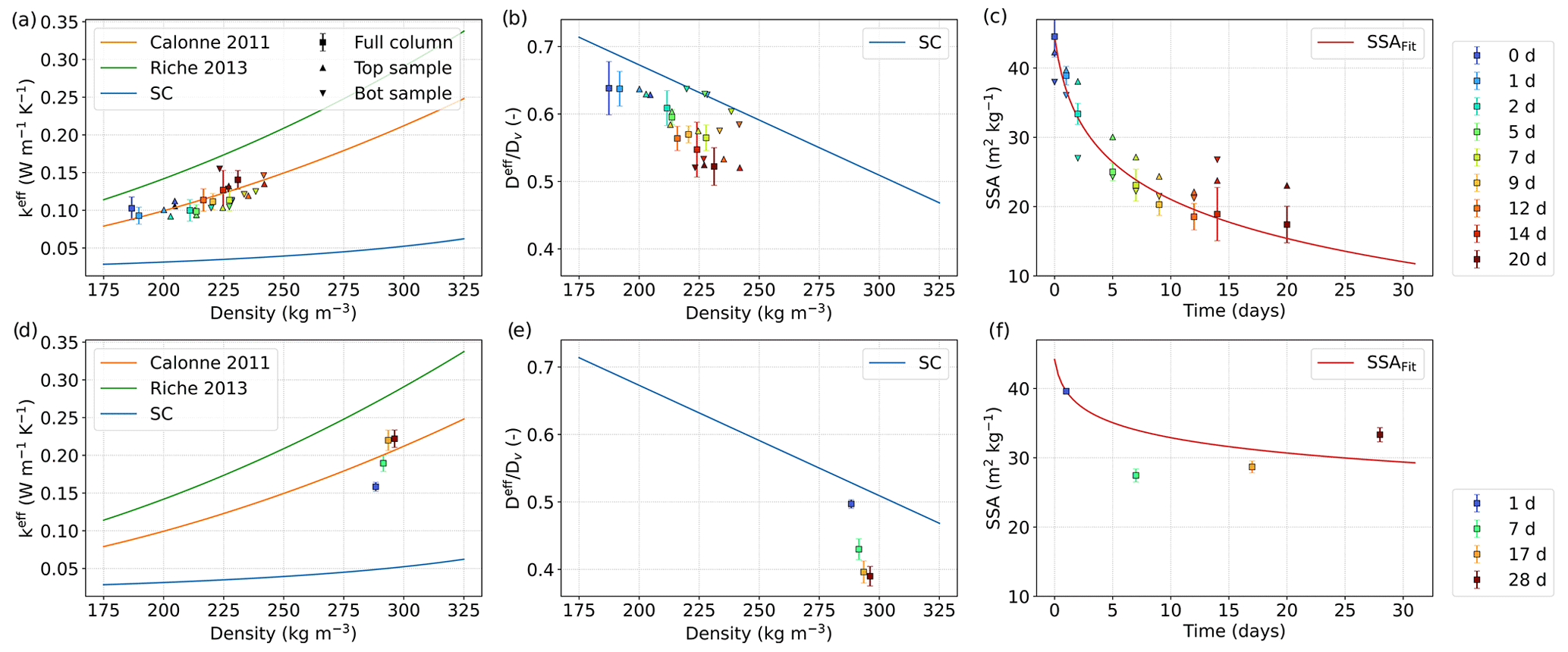
Figure 14Average values of effective conductivity and normalized effective diffusivity as a function of density and SSA as a function of time, as computed from the tomography images of Bouvet A (symbols; a–c) and Bouvet B (symbols; d–f). The error bars represent the standard deviation of the parameter along the image height. Comparison with the SC model, classical parameterizations, and fits are shown (solid lines).
Figure 14 presents the results of the image-based computations of keff, Deff, and SSA for the experiment of Bouvet A and Bouvet B. To compare them, we show the estimates of keff and Deff by the SC model presented in Sect. 3.2, the density-based parameterizations of keff from Calonne et al. (2011) and Riche and Schneebeli (2013), and a fitted regression of the SSA values as a function of time, referred as SSAFit(t), based on a logarithmic function as formerly proposed by Legagneux et al. (2004). For thermal conductivity, the parameterization of Calonne et al. (2011) is in good agreement with the image-based computations in both experiments, whereas the parameterization of Riche and Schneebeli (2013), which specifically describes the case of depth hoar, predicts slightly larger values. The SC model largely underestimates the values, which are about 2 to 4 times smaller than the image-based computations. For the vapor diffusion coefficient, the SC model provides overall fair estimates, which are slightly overestimated, especially towards the end of the experiments, as reported for depth hoar and faceted crystals in Calonne et al. (2014b). For SSA, the fit reproduces the SSA evolution well for the experiment of Bouvet A. For Bouvet B, the SSA does not follow the classic exponential decrease, but it increases after 7 d and until the end of the experiment; this increase is specific to hard-depth hoar formation (Bouvet et al., 2023). This feature is not predicted by the applied fit, yet it provides fair estimates of the SSA values.
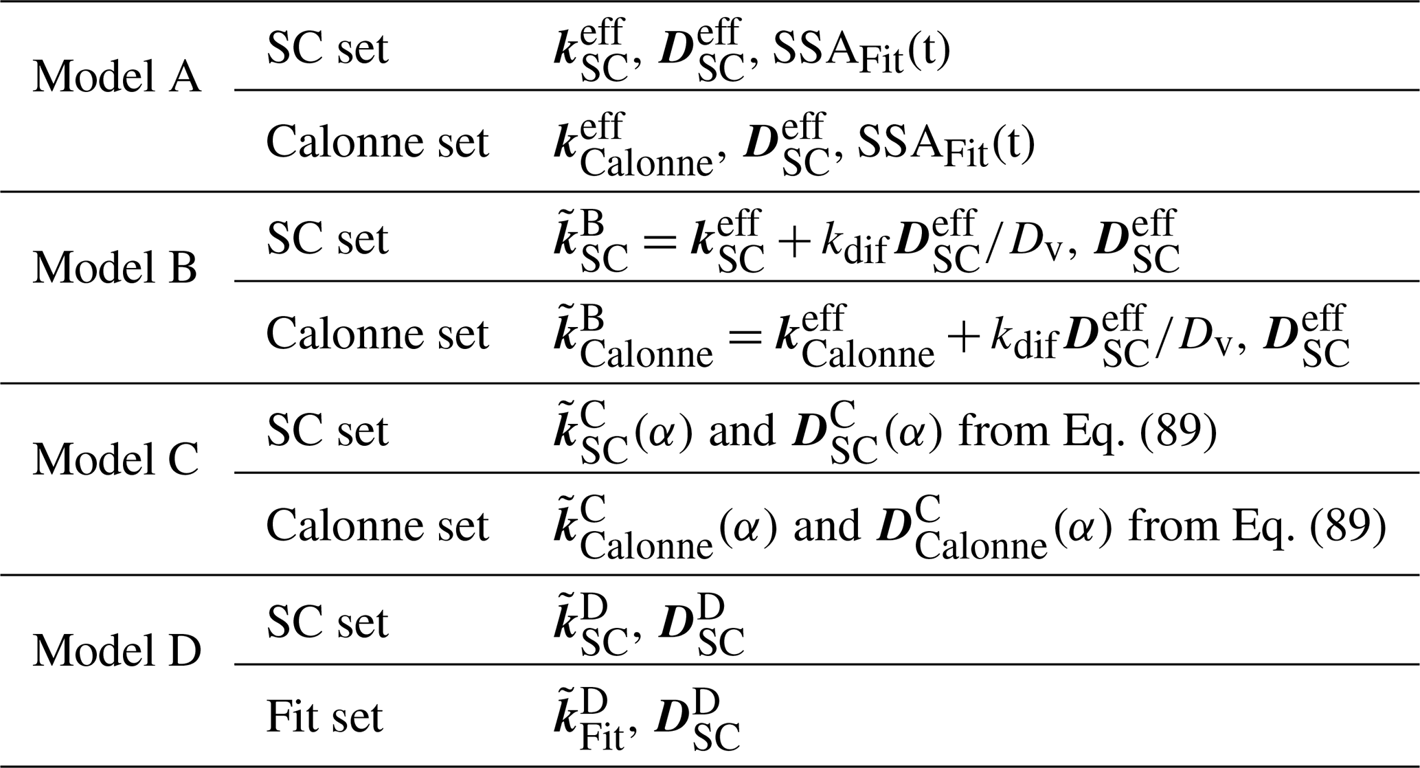
Given the above considerations, we selected two sets of parameters to simulate Bouvet A, Bouvet B, and Kamata with model A, which are summarized in Table 3. In the set called Calonne, keff is estimated with the parameterization of Calonne et al. (2011). In the second set called SC, keff is given by the self-consistent estimates. In both sets, Deff is estimated with the SC model and the SSA with the logarithmic fit, which is specific for Bouvet A and Bouvet B. In the case of the Kamata experiment, we cannot test the proposed estimates of keff, Deff, and SSA against reference data as such data are not available from Kamata and Sato (2007). The SSA evolution was reproduced based on the logarithmic fit from Bouvet A, as both experiments are the closest in terms of initial snow type, grain size, and density. In the model evaluation that follows (Sect. 4.3), the Calonne set is the one used by default to evaluate model A. Results with the SC set are also presented to illustrate an alternative choice of parameters, which, although less accurate, allows for consistent and analytically based estimates for all properties.
Table 3Summary of the effective parameters used in the simulations.
4.2.2 Models B and D
Models B and D only involve the apparent thermal conductivities of snow and , respectively. Estimating comes down to estimating keff and Deff, as it is defined as . For that reason, we use the same estimates of keff and Deff selected for model A as described above. So two sets of input parameters were used for model B, namely the Calonne set, from which the model's performances are evaluated, and the alternative SC set (Table 3). Figure 15 presents the evolution of and with temperature for each experiment, taking the mean snow density of the experiments (see Table 2). Both estimates show similar trends but, as in model A, the SC estimate predicts lower values than when using the parameterization of Calonne et al. (2011).
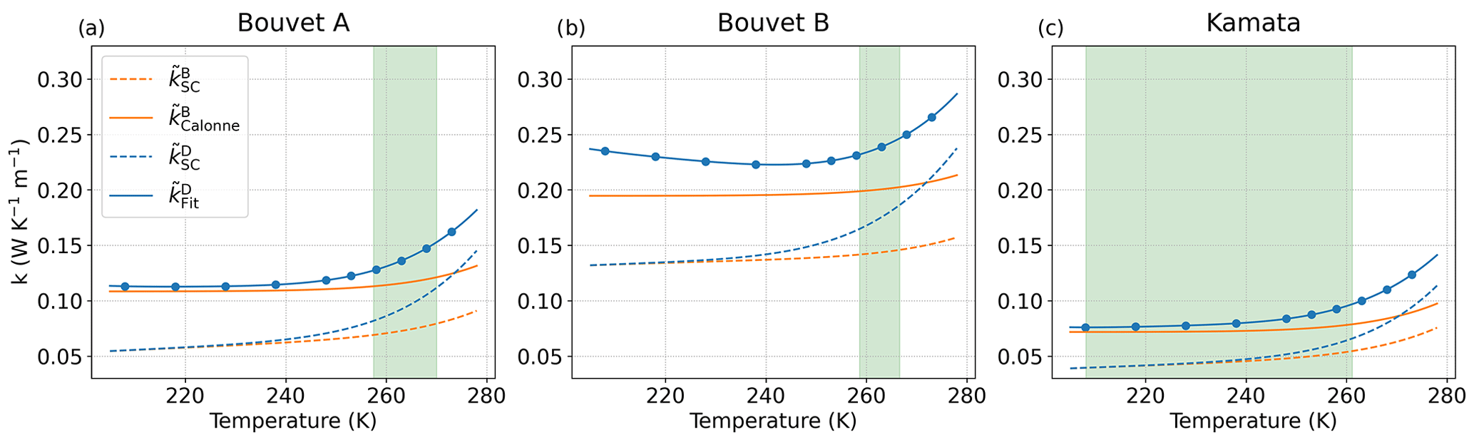
Figure 15The thermal conductivity estimates for model B ( and ) and for model D ( and ) are presented as a function of temperatures (solid and dotted lines). The parameters are presented for the Bouvet A, Bouvet B, and Kamata experiments, and the green areas represent the temperature ranges of each experiment. The computed values on 3D images used to derive are shown by blue dots. For Bouvet A, . For Bouvet B, . For Kamata, .
For model D, was computed from the 3D images from Bouvet A and Bouvet B by solving the boundary problem in Eqs. (66)–(70) with the GeoDict software. As above, only diagonal terms of the tensor were considered, and refers to the average value of the diagonal terms. Here, computations were performed on only one REV from each experiment and for 10 temperatures ranging from 210 to 273 K. We selected the image at 14 d for Bouvet A (cropped between 5.8 and 6.7 cm height) and the image at 7 d for Bouvet B (cropped between 1.7 and 2.5 cm height). To be able to estimate for the Kamata experiment, we took a 3D image of snow showing similar characteristics, namely a sample of depth hoar with a density of 165 kg m−1 from Fourteau et al. (2021a). Results of the image-based computations are presented in Fig. 15, as well as estimates from the SC model presented in Sect. 3.2. For each experiment, a fit was performed on the computed data and is referred to as in the following. Again, the SC estimates for model D capture the trend but largely underestimate the values. In what follows, simulations were performed using the fitted values , referred to as the Fit set in Table 3, upon which the evaluation of model D is based. As for the other models, simulations with the SC estimates are also presented for the sake of comparison as they allow for independent and consistent estimates.
4.3 Comparisons between models and experiments
In this section, we compare simulations from models A, B, and D with the measurements from the three experiments Bouvet A, Bouvet B, and Kamata. The simulations were performed with the software COMSOL Multiphysics by resolving the homogenized equations on a 1D geometry that corresponds to the snow layer of the experiments. We used Eqs. (21)–(22) for model A, Eqs. (41) and (37) for model B, and Eqs. (71) and (62) for model D. For model A, the boundary conditions in temperature are the top and bottom imposed temperatures of the experiments. In terms of vapor density, the conditions correspond to zero flux at the top and bottom. Additionally, the source term is forced to zero in the simulation nodes where a density of zero is reached. For models B and D, the boundary conditions are the imposed temperatures. The models were run using the sets of input parameters described in Table 3 and considering the experimental conditions summarized in Table 2. Comparisons between measurements and simulations are performed based on temperature and mass change variables.
4.3.1 Temperature
Figure 16 presents the measured and simulated vertical profiles of ΔT with models A, B, and D for the three experiments, taking different α values from 10−9 to 10−4 for model A. The ΔT values analyzed here are the ones computed at the beginning of the experiments when the temperature gradient is well established but before the formation of the air gap. Overall, profiles of ΔT have similar shapes as the ones simulated on the simplified 2D microstructure (Sect. 3.3), describing right-headed curves indicating that processes apart from heat conduction, such as phase change, occur and result in a heat source in the snow layer. In the center part of the layer, a maximum deviation of 1.15 K was measured in the Bouvet A experiment and of 5.9 K in the Kamata experiment. The negative ΔT value in the upper part of the layer in Bouvet A is attributed to the temperature sensor uncertainty (Bouvet et al., 2023).
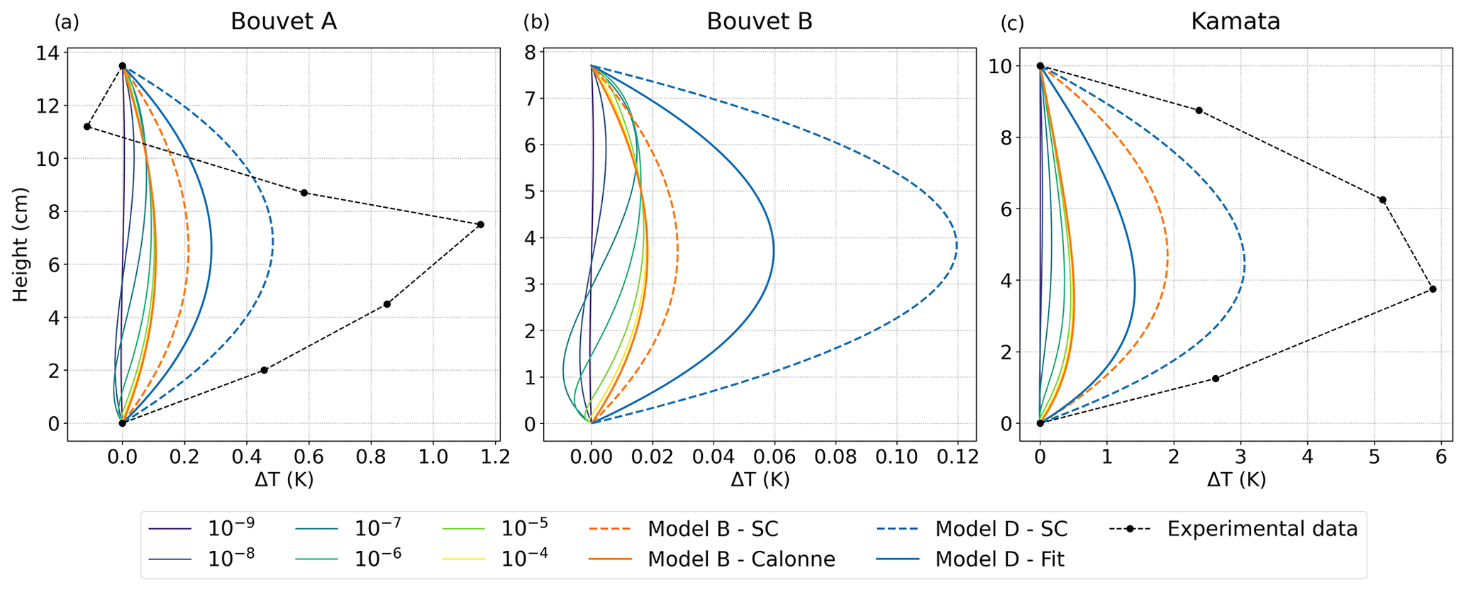
Figure 16Vertical steady-state profiles of ΔT simulated with model A, with α ranging from 10−9 to 10−4, and with models B and D for the Bouvet A, Bouvet B, and Kamata experiments. Simulations using the Calonne set (solid lines) are shown for model A, and simulations using both Calonne (solid lines) and SC sets (dashed lines) are shown for models B and D. The experimental profiles are shown with dashed black lines for Bouvet A and Kamata.
Looking at the models, the main observation is that they all underestimate ΔT. In more detail, model A predicts negative ΔT in the lower part of the snowpack and is positive otherwise, reflecting a heat sink attributed to more sublimation in the lower part and a heat source attributed to more deposition in the rest of the layer. With increasing α, the positive values of ΔT increase, and the negative ones tends to vanish, so that the shape of the simulated curve becomes closer to the experimental one. The maximum ΔT predicted by model A is reached for the highest α = 10−4 and is of 0.11 K for Bouvet A and of 0.49 K for Kamata, which corresponds only to 10 % and 8 % of the experimental value, respectively.
Models B and D show a unique ΔT profile valid over their domain of validity, namely and , respectively. The profile shape is in agreement with the measurements, showing only positive values throughout the layer. ΔT values of model B correspond to the upper limit of model A. Model D is the closest to the experimental data. Still, values are largely underestimated and reach at most 0.29 K (25 % of the experimental data) for Bouvet A and 1.4 K (23 % of the experimental data) for Kamata. In both models B and D, slightly better results are found when using the SC set of input parameters, even though it corresponds to underestimated estimates, as seen in Sect. 4.2. This better agreement with the SC estimate is somehow artificial and comes from the fact that the lower values of and , compared to and , respectively, lead to reduced overall heat conduction through snow and allow for higher ΔT, as well as the fact that the SC estimates allow for a slightly higher sensitivity (steeper slope) of the thermal conductivity to temperature in the temperature range of the considered experiments (see the green areas in Fig. 15). A final interesting point is the strong impact of the density on ΔT, which can be seen by comparing simulations of Bouvet A and Bouvet B for which temperature gradients were very close, but snow density was 210 and 287 kg m−3, respectively. For the same temperature gradient, the higher the snow density, the higher the heat conduction through snow and the lower the ΔT. For example, in lighter snow (Bouvet A), a maximum ΔT of 0.29 K is predicted by model D against 0.06 K for the denser snow (Bouvet B).
4.3.2 Mass change
Next, we evaluate the models regarding mass changes across the vertical dimension of the snow layer. We look at the vertical density profile of snow, as well as the height of the air gap formed at the base of the layer at the end of the experiments, caused by an upward mass transfer during the TGM. For model A, the air gap height is defined as the highest height value at which the density is zero. For models B, C, and D, the vertical profile of density cannot be evaluated because they only predict deposition and thus density increase, due to the boundary condition issue already described in Sect. 3.3. Still, to allow for a comparison with measurements, we derived a rough estimate of the air gap by considering that all the mass gained in the snow layer over the whole experiment duration is balanced by a mass loss localized at the very bottom of the snow layer, leading to a sharp air gap described as
with hair gap as the height of the air gap (m), H as the total height of the snow layer (m), ϕinit as the initial porosity (–), and texp as the total duration of the experiment (s) (Table 2). D is the diffusivity coefficient and corresponds to for model B and for model D. For model C, D corresponds to DC(α) using Eq. (89). The air gap for model C can also be directly calculated using only the air gap values of models B and D and a fitting function similar to Eq. (89),
with A=1200.
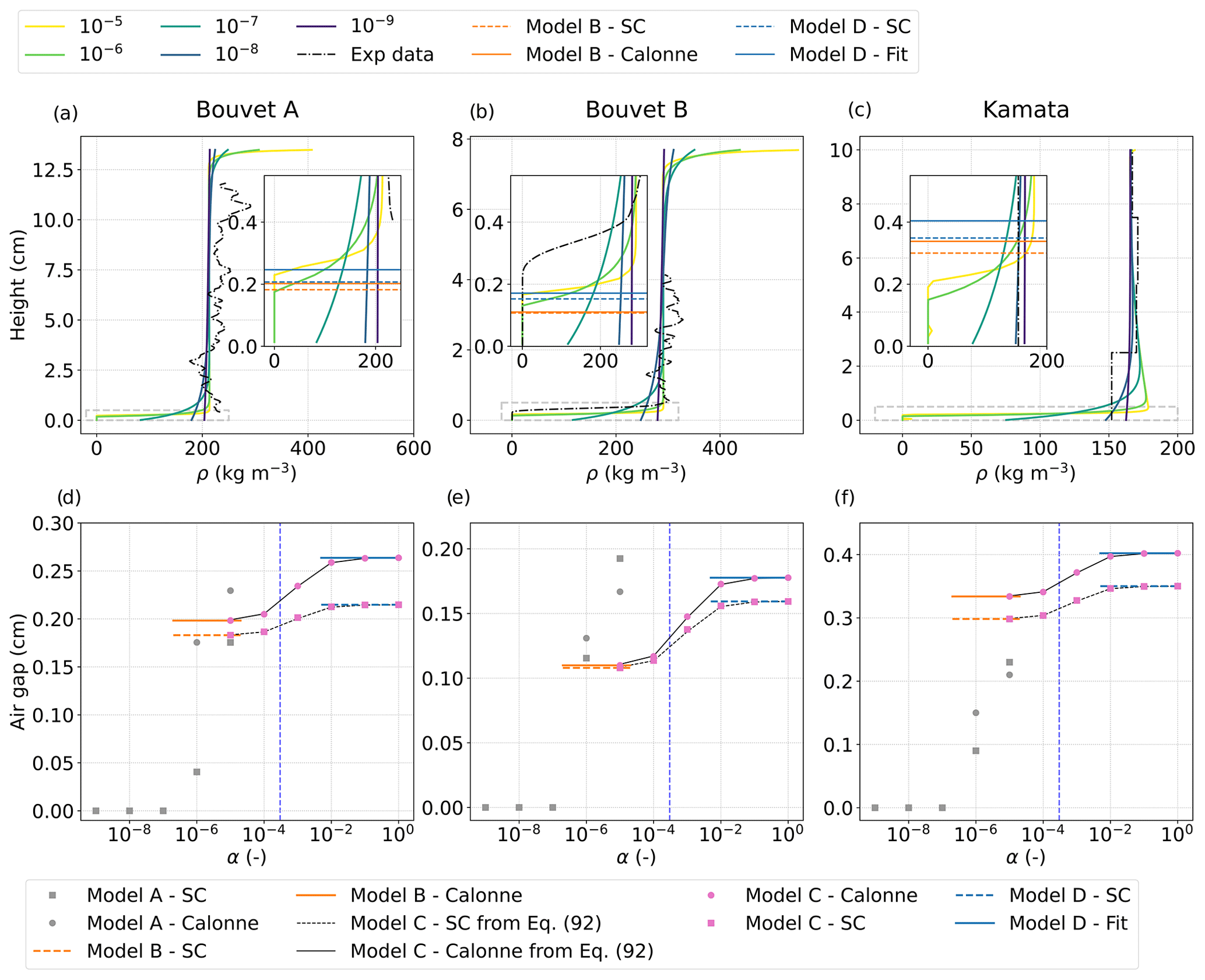
Figure 17(a, b, c) Density profiles from the macroscopic models and from the experimental data for the final stage of the Bouvet A, Bouvet B, and Kamata experiments. Results of model A are provided for α values from 10−5 to 10−9 and for the parameter set Calonne. The height of the air gaps derived for models B and D are shown with horizontal bars in the insets with an enlarged portion of the graph. Results of model B are provided for the SC set (dashed orange lines) and the Calonne set (solid orange lines). Results of model D are provided for the SC set (dashed blue lines) and the Fit set (solid blue lines). (d, e, f) Air gap height at the final stage of the experiments as a function of α, simulated with models A, B, C, and D using the parameter sets of SC, Calonne, and Fit. For model C, the air gap calculated with Eq. (92) is also shown with black lines.
Figure 17 shows the vertical profile of the density and the height of the air gap simulated and measured in Bouvet A, Bouvet B, and Kamata at the end of the experiments. The Bouvet B and Kamata experiments report a mass loss in the lower part of the snow layer. In Bouvet B, it results in the formation of an air gap of 2.7 mm height at the layer base or the point at which the snow density drops from about 290 to 0 kg m−3 within a few millimeters (Fig. 17b). In Kamata, the initial uniform density profile around 165 kg m−3 evolved and at the final stage showed a density of 152 kg m−3 at the bottom of the layer which is lower than elsewhere, where density is around 170 kg m−3 (Fig. 17c). So only a decrease in density at the base was observed and not an air gap. However, this might have been prevented by the vertical resolution of the density measurement of 2.5 cm in Kamata, at which point the detection of a millimeter-scale air gap is not possible. To provide an estimation of the height of the potential air gap, we converted the density decrease in the first 2.5 cm at the bottom into a air gap. This would lead to a 2.6 mm height air gap, similar to the one measured for Bouvet B for a much lower temperature gradient. Finally, as already mentioned, the experiment of Bouvet A does not include the first millimeters at the base of the snow layer, so a comparison with the simulations is not possible.
Looking at the experiments Bouvet A and Bouvet B, a first description of model A is given, with α ranging from 10−9 to 10−5. The model predicts similar mass transport for both experiments; there is a mass gain in the upper part of the layer and a mass loss in the lower part, with the latter feature being consistent with the measurements. In more detail, and as for temperature, the impact of α is clearly shown. For the lowest α value of 10−9, the density profile is almost linear, so the mass redistribution is even throughout the layer. As α increases, the area of mass loss and mass gain becomes more localized near the base and top of the layer, and the density transitions become sharper. From and above, an air gap is simulated with density values reaching 0 kg m−3 at the bottom. The air gap closest to the experiments is obtained with the highest and reaches 2.3 mm height for Bouvet A and 1.65 mm for Bouvet B, which corresponds fairly well to the measured air gap, yet is slightly underestimated (75 %) (Fig. 17d and e). Approximations of the air gap for models B and D are close to the ones simulated by model A so that all of the models seem to underestimate the air gap. For Bouvet B, an air gap of 1.7 mm is estimated for model D (63 % of the experimental air gap) and of 1.1 mm for model B (41 % of the experimental air gap). Finally, for all of the models, using the alternative SC set of input parameters (Table 3) has little impact on the air gap and leads mostly to a slight reduction in height (dashed lines in Fig. 17).
Simulations of the Kamata experiment with model A differ from the ones of Bouvet A and Bouvet B. Indeed, a mass gain is not predicted in the upper part of the snow layer but instead in a zone right above the mass loss region. This is particularly visible for , where the air gap, located in the first 2.1 mm, is directly surmounted by the densest part of the snow layer, located around 4 mm, with a density reaching 175 kg m−3. Simulations seem to show that the mass redistribution in the Kamata experiment occurs mostly in the lower part of the snow layer, which might be due to the impact of temperature on the simulated heat and mass transport processes so that they are reduced in the very cold upper part (−65 °C). This effect of temperature can also be seen in the simulations on the simplified microstructure for the temperature gradient of 500 K m−1 for which the imposed temperature conditions were close to the ones of Kamata, as presented in Fig. 12f. Considering that this effect applies in reality, it would imply that the final density measured in Kamata in the first 2.5 cm at the bottom is the result of both the mass loss and mass gain and thus that the above estimation of an air gap of 2.6 mm might be an underestimation. Comparisons of air gaps for the Kamata experiment should be looked at with the above consideration in mind. When averaging the simulated density values of model A over a 2.5 cm step, as done in the measurements, a value of 158 kg m−3 is found for the first 2.5 cm, in agreement with the measured one of 152 kg m−3. Coming back to the air gap comparisons, model A predicts the air gap estimated for the Kamata experiment well when the highest α value is considered. At , the simulated air gap is 2 mm; again, this close to the estimated one of 2.6 mm despite being underestimated (77 %). Unlike for Bouvet A and Bouvet B, models B and D stand out from model A, and their approximations of the air gap are significantly larger at between 3 mm and 4 mm. They would thus predict a larger air gap than the one observed in the experiment, which is up to twice the height.
5.1 Modeling heat and mass transfer with models A, B, C, or D
In the present work, macroscopic models for heat and mass transfer in dry snow have been derived by homogenization from the physics at the pore scale for different values of the condensation coefficient α in the range [10−10, 1]. The latter was assumed to be constant in the whole modeled snow layer. The Robin boundary equation for the water vapor at the ice–air interface allowed us to define a transition value αT, which equals for a typical snow grain size of around 0.5 mm that characterizes the transition between the two main mechanisms driving the water vapor transfer through the snowpack, namely diffusion and sublimation–deposition. The homogenization process allowed us (i) to retrieve three different models already proposed in the literature (Calonne et al., 2014b; Hansen and Foslien, 2015; Moyne et al., 1988); to specify their domains of validity according to the α values; and (ii) to show that the hypothesis ρv=ρvs(T), which is often made, is a good approximation for α values larger than 10−6.
At the macroscopic scale, model A (Calonne et al., 2014b), valid for α values in the range [10−10, 10−5], is described by two coupled equations, with one for the temperature field and one for the water vapor field. They are coupled by a source term that reflects the sublimation–deposition process and depends on α. In this model, the induced porosity variation in the snow layer can be easily computed. In the case of models B, C, and D (Moyne et al., 1988; Hansen and Foslien, 2015), the physics at the macro-scale is driven by the temperature field only as ρv=ρvs(T). Because the models only solve the temperature field, it is not as straightforward to access the porosity variation. In our case, both models do not satisfy mass conservation and predict only the deposition over the whole snow layer and also the sublimation front occurring at the bottom of the snow layer, as seen in the comparison between pore-scale and macroscopic-scale simulations (Fig. 12). In the future, a more reliable boundary condition, such as a Stefan boundary condition, should be introduced to better describe the evolution of the sublimation front.
According to their definition, models B and D do not depend on α and are able to describe the observed plateaus in a limited range of α. These two models can be seen as particular cases of models A and C. Consequently, in practice, models A and C, which depend on α, are sufficient to describe the macroscopic heat and mass transfer through the snowpack for α values in the range 10−10 to 1. Let us remark that model C requires solving a fully coupled problem at the REV scale in order to determine the effective parameters.
5.2 On the comparisons between simulations and measurements
5.2.1 Summary of the models' evaluation
When comparing experiments and simulations with the three models, it appears that they are able to reproduce the main features of the heat and mass transport during the TGM, including the non-linear temperature profile and, for model A, the upward vapor transport with, eventually, the formation of a millimeter-scale basal air gap. However, a major discrepancy lies in the fact that temperature values are underestimated by all the models. More precisely, the heat source inducing the non-linearity in the temperature profile seems underestimated. The best predictions of the temperature deviation ΔT are obtained by model D and correspond to only about 25 % of the experimental data, translating into temperature differences of around 1 and 5 K for the Bouvet A and Kamata experiments, respectively. To a much lesser extent, upward vapor transport seems slightly underestimated, and the heights of the basal air gaps simulated by model A correspond to about 75 % of the experimental ones, leading to small differences in height of 1 and 0.6 mm for the Bouvet B and Kamata experiments, respectively. Similar conclusions can be drawn for models B and D, based on rough approximations of the air gap. Possible causes of the differences between experiments and simulations are explored in the following.
5.2.2 Uncertainties in the experimental data
Temperature measurements in Bouvet A were performed with Pt100 sensors with an accuracy of ±0.2 °C (Bouvet et al., 2023). Copper Constantan thermocouples were used in the experiment of Kamata and Sato (2007) and are known to be very stable at low temperatures, with an accuracy of ±0.5 °C. In both cases, these uncertainties are smaller than the discrepancies between the measured and modeled ΔT. For density, the experimental setup of Bouvet B ensures precise monitoring of the mass change over time by tomography (Bouvet et al., 2023). Air gaps similar to the one in Bouvet B were reported by Wiese (2017) during temperature gradient experiments. For the Kamata experiment, the reliability of the compartment method is less obvious, and the vertical resolution of 2.5 cm is rather poor to assess the presence of an air gap.
5.2.3 Uncertainties in the numerical simulation input
The macroscopic modeling of heat and mass transport in dry snow relies on the effective parameters of keff, Deff, and the SSA for model A; on for model B; and on for model D. For thermal conductivity, the different estimates used in the simulations are overall in good agreement with the values computed from the experimental 3D images. A possible way to improve could be to account for the anisotropy of the property so that there is, e.g., an enhanced thermal conductivity in the vertical direction, as observed for snow evolving under a high TGM (e.g., Calonne et al., 2011). However, an increase in the thermal conductivity of models A, B, and D leads to a decrease in both the temperature deviation and air gap height and thus a degradation in the model performance, as illustrated in Fig. 16. Concerning the vapor diffusion coefficient, the SC models were used in the simulations, which provide slightly overestimated estimates. However, improving these estimates, through taking lower values of the diffusion coefficient, leads to a decrease in both temperature deviation and air gap height, which, again, degrades the model results. To illustrate this behavior in the case of model A, by lowering the SC estimate of Deff by 10 %, a ΔT of 0.096 K and an air gap of 1.17 mm is simulated for , compared to 0.102 K and 2.3 mm with the initial value. Finally, potential errors in the SSA parameter would affect the source term of model A and would only translate in small variations in α. To conclude, the uncertainties linked to the estimation of the effective parameters cannot be responsible for the reported differences between experiments and simulations.
5.2.4 Models limitations and potential improvements
As the points raised above do not seem sufficient to explain the model errors, a plausible cause remains to be investigated and is the definition of the model itself, i.e., the definition of the physics at the pore scale considered for the homogenization. A first element concerns the source terms in model A, which are derived from the Hertz–Knudsen equation and rely on a condensation coefficient α (Eq. 7). Here, this coefficient was taken to be constant and uniform over the snow layer and considered equal for both condensation and sublimation. In their review, Persad and Ward (2016) explore the expressions of the evaporation coefficient and of the condensation coefficient in the Hertz–Knudsen equation for the water–air interface. They conclude that most errors come from assuming the evaporation and condensation coefficients to be equal and assuming thermal equilibrium across the liquid–vapor interface (Eq. 4 in this study). Moreover, as mentioned in the Introduction, the condensation parameter α depends on many parameters, such as the vapor supersaturation, which can lead to a non-linear expression of the Hertz–Knudsen equation. Hence, refining the Hertz–Knudsen equation could add non-linearity in the source terms of model A, which could enhance the contribution of latent heat and thus increase the temperature deviation ΔT, which would improve the model's prediction.
Another point is that the natural convection was not taken into account at the pore scale. This process was, however, hypothesized to be key for heat and mass transport of snow under strong temperature gradients, such as Arctic and sub-Arctic ones (e.g., Sturm and Johnson, 1991; Domine et al., 2018). To include natural convection, fluxes of temperature (JT) and water vapor () should be expressed at the pore scale as follows:
with va as the air velocity. A numerical study was recently presented by Jafari et al. (2022) using a macroscopic model similar to model A. They show that the occurrence and intensity of natural convection in snow depends on the Rayleigh number, which is defined as
where H is the height of the snow layer, K is the snow permeability, g=9.81 m s−2 is the gravity, Pa s is the air viscosity, and βT=0.0036 K−1 is the thermal expansion coefficient. Their simulations indicate that, for Ra>50 and H>25 cm, the natural convection could generate an upward air flux from the warmer region to the colder one, and vice versa. We estimated the Rayleigh number for the three experiments used in this study. Using the values in Tables 1 and 2, and using the parameterization of Calonne et al. (2012) for the snow permeability, the Rayleigh number is typically 0.15, 0.02, and 0.85 for the experiments Bouvet A, Bouvet B and Kamata, respectively. These values are much smaller than the threshold value presented by Jafari et al. (2022), which would indicate that natural convection is negligible in our cases. Moreover, Kamata et al. (1999) present a symmetric TGM experiment with warmer conditions at the base and top of the snow layer and colder conditions imposed in the middle using a cold plate. The snow layer was thus under a positive TG in one part and under a negative TG in the other part, with both having the same intensity. The temperature profiles were recorded in both parts of the snow layer and show similar non-linear curves in both cases, although natural convection could only occur in the bottom area, where the temperature conditions are unstable. The authors conclude that natural convection does not seem to impact their temperature fields. This would be consistent with the small Rayleigh number that we estimated to be 0.16 for this experiment.
Finally, the cross-coupling effects between the temperature and water vapor density, such as the Soret and Dufour effects, were not considered in the physics at the pore scale. The effect of the vapor density gradient on the heat flux, called the Dufour effect, is characterized by the thermodiffusion coefficient DTv, and the effect of temperature gradient on the vapor density flux, called the Soret effect, is characterized by the thermodiffusion coefficient DvT. Taking these effects into account, the temperature and water vapor flux can be expressed as follows:
For porous media, the Dufour effect is neglected in most cases, whereas the Soret effect is often taken into account (e.g., Davarzani et al., 2010; Häussling Löwgren et al., 2020) and can be measured using the Soret coefficient defined as . This coefficient is positive when the heaviest species in the pore space move toward the colder regions and is negative when they move toward the warmer regions. However, this coefficient could change sign when the temperature is lowered (Caldwell, 1973; Chapman and Cowling, 1990). When the temperature is positive, the Soret coefficient for water vapor is supposed to be positive. To the best of our knowledge, there are no data concerning this coefficient when temperature is negative. The Soret effect can be easily introduced in pore-scale simulations in the case of the 2D simplified microstructure as presented in Sect. 3.3. By doing so, we found that negative ST coefficients lead to an increase the simulated temperature deviation ΔT, and vice versa. For example, for α=0.1 and a temperature gradient of 500 K m−1, a maximum value of ΔT of 6.5, 4.2, and 2.8 K is simulated for ST equal to −2 × 10⁻⁴, 0, and 2 × 10⁻⁴, respectively. The Soret effect can also be introduced in model D, by replacing ka+kdiff with . Using the self-consistent estimate of thermal conductivity (Eq. 87) and for values of ST at −2 × 10⁻⁴, 0, and 2 × 10⁻⁴, the maximum simulated values of ΔT for the Kamata experiment are 6.3, 3.1, and 1.95 K, respectively, whereas the experimental value is around 6 K. A negative Soret coefficient seems thus suitable to improve the temperature simulations and better describe the experimental data. However, the influence of the Soret effect on the air gap is not straightforward, as it seems to induce a downward movement of vapor molecules and is thus opposed to the formation of a basal air gap. These preliminary results show that the introduction of such coupling effects (Soret and/or Dufour) between the temperature and the water vapor density in the modeling of heat and water vapor transfer in snowpacks is interesting and that future work would be needed to investigate such a hypothesis.
This paper presents the definition and evaluation of the equivalent macroscopic modeling of heat and mass transport during the TGM in dry snow. First, we applied the homogenization process to retrieve the macroscopic models valid for condensation coefficients α ranging from 10−10 to 1. We showed that, at a transition value , the modeling changes from vapor transport limited by sublimation–deposition (models A and B) to vapor transport limited by diffusion (model D). The homogenization process allowed us to retrieve different models proposed in the literature (Calonne et al., 2014b; Hansen and Foslien, 2015; Moyne et al., 1988) and to clarify their domains of validity according to the value of α. Models A and C are sufficient to describe the heat and mass transfer in the whole range of α values between 10−10 and 1. For α values between 10−10 and 10−5, model A consists of two equations of temperature and water vapor density coupled through the source terms, which are proportional to the Hertz–Knudsen equation and therefore to α. This model does not presume any assumption on the saturation of the vapor density. For α values between 10−5 and 1, model C consists of one temperature equation which involves α, since the hypothesis ρv=ρvs(T), which is often made, is valid in that range. Concerning the two other models, model B can be seen as a particular case of model A for α values in the range from 10−7 to 10−5, whereas model D can be seen as a particular case of model C for α values in the range from 10−3 to 1.
In the second part of the paper, we evaluated the homogenized models A, B, C, and D by comparison with three laboratory experiments of the TGM of snow (Kamata and Sato, 2007; Bouvet et al., 2023), as well as by a numerical evaluation for a 2D simplified microstructure. Evaluations were performed based on the temperature and density profiles of snow and, more precisely, on the ability to reproduce two main features reported in the TGM experiments, namely the non-linear concave-shaped temperature profile, characterized by the temperature deviation from a linear gradient ΔT, and the upward vapor transport leading to a mass loss or an air gap at the base of the snow layer. We showed that (i) the four models allow the reproduction of the shape of the temperature profile, but the values were largely underestimated, with the best prediction being obtained with model D and corresponding only to 25 % of the temperature difference observed in the experimental data. This major discrepancy highlights that a process that contributes to heat up the layer is not well captured, if at all; (ii) model A allows us to reproduce the upward vapor transport and the formation of a millimeter-scale basal air gap, with the best result being obtained for the highest α value of 10−5; and (iii) models B and D (and also C) do not allow the reproduction of mass transport as they predict only the mass gain in the snow layer and as they do not satisfy mass conservation in the present case. Potential improvements were suggested and include the refining or enrichment of the physics at the pore scale considered to derive the models, such as questioning the expression of the Hertz–Knudsen equation or the role of the Soret and/or Dufour effects, as well as improving the boundary conditions to allow for realistic mass transport for models B, C, and D.
The theoretical development of the macroscopic equivalent descriptions are available in the Supplement.
The supplement related to this article is available online at: https://doi.org/10.5194/tc-18-4285-2024-supplement.
CG, NC, and LB conducted the derivation of the macroscopic models. LB applied the models to the experimental data. The analyses and interpretations were carried out by LB, FF, NC, and CG. LB and CG prepared the paper, with contributions from all co-authors.
The contact author has declared that none of the authors has any competing interests.
Publisher’s note: Copernicus Publications remains neutral with regard to jurisdictional claims made in the text, published maps, institutional affiliations, or any other geographical representation in this paper. While Copernicus Publications makes every effort to include appropriate place names, the final responsibility lies with the authors.
We warmly thank the editor, Jürg Schweizer, and the reviewers, Tien Dung Le and the anonymous reviewer, for their insightful comments which helped to significantly improve the quality of the paper.
The 3SR lab is part of the Labex Tec 21 (Investissements d’Avenir; grant no. ANR-11-LABX-0030). CNRM/CEN is part of Labex OSUG@2020 (Investissements d’Avenir; grant no. ANR-10-LABX-0056). This research has been supported by the Agence Nationale de la Recherche through the MiMESis-3D ANR project (grant no. ANR-19-CE01-0009).
This paper was edited by Jürg Schweizer and reviewed by Tien Dung Le and one anonymous referee.
Albert, M. R. and McGilvary, W. R.: Thermal effects due to air flow and vapor transport in dry snow, J. Glaciol., 38, 273–281, https://doi.org/10.3189/S0022143000003683, 1992. a, b
Anderson, E. A.: A point energy and mass balance model of a snow cover, Tech. Rep., Office of Hydrology – National Weather Service, https://repository.library.noaa.gov/view/noaa/6392 (last access: 16 July 2024), 1976. a
Auriault, J.-L.: Heterogeneous medium. Is an equivalent description possible?, Int. J. Eng. Sci., 29, 785–795, https://doi.org/10.1016/0020-7225(91)90001-J, 1991. a, b, c, d, e
Auriault, J.-L., Boutin, C., and Geindreau., C.: Homogenization of coupled phenomena in heterogenous media, Wiley-ISTE, London, https://doi.org/10.1002/9780470612033, 2009. a, b, c
Barrett, J. W., Garcke, H., and Nürnberg, R.: Numerical computations of faceted pattern formation in snow crystal growth, Phys. Rev. E, 86, 011604, https://doi.org/10.1103/PhysRevE.86.011604, 2012. a
Bensoussan, A., Lions, J.-L., and Papanicolaou, G.: Asymptotic Analysis for periodic structures, North Holland, https://www.ams.org/books/chel/374/chel374-endmatter.pdf (last access: 16 July 2024), 1978. a, b, c, d
Bouvet, L., Calonne, N., Flin, F., and Geindreau, C.: Snow equi-temperature metamorphism described by a phase-field model applicable on micro-tomographic images: Prediction of microstructural and transport properties, J. Adv. Model. Earth Sy., 14, e2022MS002998, https://doi.org/10.1029/2022MS002998, 2022. a, b
Bouvet, L., Calonne, N., Flin, F., and Geindreau, C.: Heterogeneous grain growth and vertical mass transfer within a snow layer under a temperature gradient, The Cryosphere, 17, 3553–3573, https://doi.org/10.5194/tc-17-3553-2023, 2023. a, b, c, d, e, f, g, h, i
Bruggeman, V. D.: Berechnung verschiedener physikalischer Konstanten von heterogenen Substanzen. I. Dielektrizitätskonstanten und Leitfähigkeiten der Mischkörper aus isotropen Substanzen, Annalen der Physik, 416, 636–664, https://doi.org/10.1002/andp.19354160705, 1935. a
Brzoska, J.-B., Flin, F., and Barckicke, J.: Explicit iterative computation of diffusive vapour field in the 3-D snow matrix: preliminary results for low flux metamorphism, Ann. Glaciol., 48, 13–18, https://doi.org/10.3189/172756408784700798, 2008. a, b
Budiansky, B.: On the elastic moduli of some heterogeneous materials, J. Mech. Phys. Solids, 13, 223–227, https://doi.org/10.1016/0022-5096(65)90011-6, 1965. a
Caldwell, D. R.: Measurement of negative thermal diffusion coefficients by observing the onset of thermohaline convection, J. Phys. Chem., 77, 2004–2008, https://doi.org/10.1021/j100635a018, 1973. a
Calonne, N., Flin, F., Morin, S., Lesaffre, B., Rolland du Roscoat, S., and Geindreau, C.: Numerical and experimental investigations of the effective thermal conductivity of snow, Geophys. Res. Lett., 38, L23501, https://doi.org/10.1029/2011GL049234, 2011. a, b, c, d, e, f
Calonne, N., Geindreau, C., Flin, F., Morin, S., Lesaffre, B., Rolland du Roscoat, S., and Charrier, P.: 3-D image-based numerical computations of snow permeability: links to specific surface area, density, and microstructural anisotropy, The Cryosphere, 6, 939–951, https://doi.org/10.5194/tc-6-939-2012, 2012. a
Calonne, N., Flin, F., Geindreau, C., Lesaffre, B., and Rolland du Roscoat, S.: Study of a temperature gradient metamorphism of snow from 3-D images: time evolution of microstructures, physical properties and their associated anisotropy, The Cryosphere, 8, 2255–2274, https://doi.org/10.5194/tc-8-2255-2014, 2014a. a, b
Calonne, N., Geindreau, C., and Flin, F.: Macroscopic modeling for heat and water vapor transfer in dry snow by homogenization, J. Phys. Chem. B, 118, 13 393–13 403, https://doi.org/10.1021/jp5052535, 2014b. a, b, c, d, e, f, g, h, i, j, k, l, m, n, o, p
Calonne, N., Geindreau, C., and Flin, F.: Macroscopic modeling of heat and water vapor transfer with phase change in dry snow based on an upscaling method: Influence of air convection, J. Geophys. Res.-Earth, 120, 2476–2497, https://doi.org/10.1002/2015JF003605, 2015. a, b
Calonne, N., Milliancourt, L., Burr, A., Philip, A., Martin, C. L., Flin, F., and Geindreau, C.: Thermal Conductivity of Snow, Firn, and Porous Ice From 3-D Image-Based Computations, Geophys. Res. Lett., 46, 13079–13089, https://doi.org/10.1029/2019GL085228, 2019. a
Chapman, S. and Cowling, T. G.: The mathematical theory of non-uniform gases: an account of the kinetic theory of viscosity, thermal conduction and diffusion in gases, Cambridge university press, ISBN 9780521408448, 1990. a
Davarzani, H., Marcoux, M., and Quintard, M.: Theoretical predictions of the effective thermodiffusion coefficients in porous media, Int. J. Heat Mass Tran., 53, 1514–1528, https://doi.org/10.1016/j.ijheatmasstransfer.2009.11.044, 2010. a
de Quervain, M.: On the metamorphism of snow, in: Ice and Snow, edited by: Kingery, W., MIT Press, 377–390, https://www.umr-cnrm.fr/IMG/pdf/dequervain_1963_on_the_metamorphism_of_snow.pdf (last access: 16 July 2024), 1963. a
Delaney, L., Houston, R., and Eagleton, L.: The rate of vaporization of water and ice, Chem. Eng. Sci., 19, 105–114, https://doi.org/10.1016/0009-2509(64)85115-0, 1964. a
Domine, F., Belke-Brea, M., Sarrazin, D., Arnaud, L., Barrere, M., and Poirier, M.: Soil moisture, wind speed and depth hoar formation in the Arctic snowpack, J. Glaciol., 64, 990–1002, https://doi.org/10.1017/jog.2018.89, 2018. a
Domine, F., Picard, G., Morin, S., Barrere, M., Madore, J.-B., and Langlois, A.: Major issues in simulating some arctic snowpack properties using current detailed snow physics models: consequences for the thermal regime and water budget of permafrost, J. Adv. Model. Earth Sy., 11, 34–44, https://doi.org/10.1029/2018MS001445, 2019. a
Dumont, M., Flin, F., Malinka, A., Brissaud, O., Hagenmuller, P., Lapalus, P., Lesaffre, B., Dufour, A., Calonne, N., Rolland du Roscoat, S., and Ando, E.: Experimental and model-based investigation of the links between snow bidirectional reflectance and snow microstructure, The Cryosphere, 15, 3921–3948, https://doi.org/10.5194/tc-15-3921-2021, 2021. a
Fierz, C., Armstrong, R. L., Durand, Y., Etchevers, P., Greene, E., McClung, D. M., Nishimura, K., Satyawali, P. K., and Sokratov, S. A.: The international classification for seasonal snow on the ground, IHP-VII Technical Documents in Hydrology, IACS Contribution no. 1, 83, https://unesdoc.unesco.org/ark:/48223/pf0000186462 (last access: 16 July 2024), 2009. a
Flin, F.: Description physique des métamorphoses de la neige à partir d'images de microstructures 3D naturelles obtenues par microtomographie X, PhD thesis, Université Joseph Fourier, Grenoble, http://www.theses.fr/2004GRE10006 (last access: 16 July 2024), 2004. a
Flin, F. and Brzoska, J.-B.: The temperature gradient metamorphism of snow: vapour diffusion model and application to tomographic images, Ann. Glaciol., 49, 17–21, https://doi.org/10.3189/172756408787814834, 2008. a, b
Flin, F., Brzoska, J.-B., Lesaffre, B., Coléou, C., and Pieritz, R. A.: Full three-dimensional modelling of curvature-dependent snow metamorphism: first results and comparison with experimental tomographic data, J. Phys. D Appl. Phys., 36, A49–A54, https://doi.org/10.1088/0022-3727/36/10A/310, 2003. a, b
Flin, F., Lesaffre, B., Dufour, A., Gillibert, L., Hasan, A., Rolland du Roscoat, S., Cabanes, S., and Puglièse, P.: On the computations of specific surface area and specific grain contact area from snow 3D images, in: Physics and Chemistry of Ice, edited by: Furukawa, Y., Hokkaido University Press, Sapporo, Japan, 321–328, http://www.umr-cnrm.fr/IMG/pdf/flin_etal_2011_ssa_sgca_published_color.pdf (last access: 16 July 2024), 2011. a
Fourteau, K., Domine, F., and Hagenmuller, P.: Impact of water vapor diffusion and latent heat on the effective thermal conductivity of snow, The Cryosphere, 15, 2739–2755, https://doi.org/10.5194/tc-15-2739-2021, 2021a. a, b, c, d, e, f, g, h
Fourteau, K., Domine, F., and Hagenmuller, P.: Macroscopic water vapor diffusion is not enhanced in snow, The Cryosphere, 15, 389–406, https://doi.org/10.5194/tc-15-389-2021, 2021b. a, b, c, d
Furukawa, Y.: 25 – Snow and Ice Crystal Growth, in: Handbook of Crystal Growth, 2nd edn., edited by: Nishinaga, T., Elsevier, Boston, 1061–1112, ISBN 978-0-444-56369-9, https://doi.org/10.1016/B978-0-444-56369-9.00025-3, 2015. a, b, c
Granger, R., Flin, F., Ludwig, W., Hammad, I., and Geindreau, C.: Orientation selective grain sublimation–deposition in snow under temperature gradient metamorphism observed with diffraction contrast tomography, The Cryosphere, 15, 4381–4398, https://doi.org/10.5194/tc-15-4381-2021, 2021. a
Hansen, A. C. and Foslien, W. E.: A macroscale mixture theory analysis of deposition and sublimation rates during heat and mass transfer in dry snow, The Cryosphere, 9, 1857–1878, https://doi.org/10.5194/tc-9-1857-2015, 2015. a, b, c, d, e, f, g
Häussling Löwgren, B., Bergmann, J., and Alves-Filho, O.: A Numerical Implementation of the Soret Effect in Drying Processes, ChemEngineering, 4, 13, https://doi.org/10.3390/chemengineering4010013, 2020. a
Haynes, W. M.: CRC handbook of chemistry and physics, CRC press, https://doi.org/10.1201/9781315380476, 2016. a, b
Hill, R.: A self-consistent mechanics of composite materials, J. Mech. Phys. Solids, 13, 213–222, https://doi.org/10.1016/0022-5096(65)90010-4, 1965. a
Huang, W., Li, Z., Liu, X., Zhao, H., Guo, S., and Jia, Q.: Effective thermal conductivity of reservoir freshwater ice with attention to high temperature, Ann. Glaciol., 54, 189–195, https://doi.org/10.3189/2013AoG62A075, 2013. a, b
Jafari, M., Sharma, V., and Lehning, M.: Convection of water vapour in snowpacks, J. Fluid Mech., 934, A38, https://doi.org/10.1017/jfm.2021.1146, 2022. a, b, c
Jordan, R.: A one-dimensional temperature model for a snow cover: technical documentation for SNTHERM.89., Tech. Rep. 91-16, U.S. Army Cold Regions Research and Engineering Laboratory, http://hdl.handle.net/11681/11677 (last access: 16 July 2024), 1991. a
Kaempfer, T. U. and Plapp, M.: Phase-field modeling of dry snow metamorphism, Phys. Rev. E, 79, 031502, https://doi.org/10.1103/PhysRevE.79.031502, 2009. a, b, c, d, e, f
Kamata, Y. and Sato, A.: Water-vapor transport in snow with high temperature gradient, in: Physics and Chemistry of Ice, edited by: Kuhs, W. F., 281–288, http://www.umr-cnrm.fr/IMG/pdf/kamata_and_sato_2007_high_tg.pdf (last access: 16 July 2024), 2007. a, b, c, d, e, f, g, h
Kamata, Y., Sokratov, S. A., and Sato, A.: Temperature and temperature gradient dependence of snow recrystallization in depth hoar snow, in: Advances in Cold-Region Thermal Engineering and Sciences, edited by: Hutter, K., Wang, Y., and Beer, H., Springer Berlin Heidelberg, 395–402, https://doi.org/10.1007/BFb0104197, 1999. a
Krol, Q. and Löwe, H.: Analysis of local ice crystal growth in snow, J. Glaciol., 62, 378–390, https://doi.org/10.1017/jog.2016.32, 2016. a, b
Legagneux, L., Taillandier, A.-S., and Domine, F.: Grain growth theories and the isothermal evolution of the specific surface area of snow, J. Appl. Phys., 95, 6175–6184, https://doi.org/10.1063/1.1710718, 2004. a
Lehning, M., Bartelt, P., Brown, B., and Fierz, C.: A physical SNOWPACK model for the Swiss avalanche warning Part III: meteorological forcing, thin layer formation and evaluation, Cold Reg. Sci. Technol., 35, 169–184, https://doi.org/10.1016/S0165-232X(02)00072-1, 2002. a
Libbrecht, K. G.: The physics of snow crystals, Rep. Prog. Phys., 68, 855–895, https://doi.org/10.1088/0034-4885/68/4/R03, 2005. a, b, c, d
Libbrecht, K. G.: A taxonomy of snow crystal growth behaviors: 1. Using c-axis ice needles as seed crystals, arXiv [preprint], https://doi.org/10.48550/ARXIV.2109.00098, 2021. a
Libbrecht, K. G. and Rickerby, M. E.: Measurements of surface attachment kinetics for faceted ice crystal growth, J. Cryst. Growth, 377, 1–8, https://doi.org/10.1016/j.jcrysgro.2013.04.037, 2013. a, b, c, d
Massman, W.: A review of the molecular diffusivities of H2O, CO2, CH4, CO, O3, SO2, NH3, N2O, NO, and NO2 in air, O2 and N2 near STP, Atmos. Environ., 32, 1111–1127, https://doi.org/10.1016/S1352-2310(97)00391-9, 1998. a, b
Moyne, C., Batsale, J.-C., and Degiovanni, A.: Approche expérimentale et théorique de la conductivité thermique des milieux poreux humides – II. Théorie, Int. J. Heat Mass Tran., 31, 2319–2330, https://doi.org/10.1016/0017-9310(88)90163-9, 1988. a, b, c, d, e, f, g
Persad, A. H. and Ward, C. A.: Expressions for the Evaporation and Condensation Coefficients in the Hertz-Knudsen Relation, Chem. Rev., 116, 7727–7767, https://doi.org/10.1021/acs.chemrev.5b00511, 2016. a
Pinzer, B. R., Schneebeli, M., and Kaempfer, T. U.: Vapor flux and recrystallization during dry snow metamorphism under a steady temperature gradient as observed by time-lapse micro-tomography, The Cryosphere, 6, 1141–1155, https://doi.org/10.5194/tc-6-1141-2012, 2012. a
Powers, D., O'Neill, K., and Colbeck, S. C.: Theory of Natural Convection in Snow, J. Geophys. Res., 90, 10641–10649, https://doi.org/10.1029/JD090iD06p10641, 1985. a
Riche, F. and Schneebeli, M.: Thermal conductivity of snow measured by three independent methods and anisotropy considerations, The Cryosphere, 7, 217–227, https://doi.org/10.5194/tc-7-217-2013, 2013. a, b
Sanchez-Palencia, E.: Non-homogeneous media and vibration theory, in: Lectures Notes in Physics, vol. 127, Springer-Verlag, Berlin, https://doi.org/10.1007/3-540-10000-8, 1980. a, b, c, d
Srivastava, P., Mahajan, P., Satyawali, P., and Kumar, V.: Observation of temperature gradient metamorphism in snow by X-ray computed microtomography: measurement of microstructure parameters and simulation of linear elastic properties, Ann. Glaciol., 51, 73–82, https://doi.org/10.3189/172756410791386571, 2010. a
Sturm, M. and Benson, C. S.: Vapor transport, grain growth and depth-hoar development in the subarctic snow, J. Glaciol., 43, 42–59, https://doi.org/10.3189/S0022143000002793, 1997. a
Sturm, M. and Johnson, J.: Natural convection in the subarctic snow cover, J. Geophys. Res.-Sol. Ea., 96, 11657–11671, https://doi.org/10.1029/91JB00895, 1991. a
Thoemen, H., Walther, T., and Wiegmann, A.: 3D simulation of macroscopic heat and mass transfer properties from the microstructure of wood fibre networks, Comp. Sci. Techn., 68, 608–616, https://doi.org/10.1016/j.compscitech.2007.10.014, 2008. a
Torquato, S.: Random Heterogeneous Materials: Microstructure and Macroscopic Properties, Springer, https://doi.org/10.1115/1.1483342, 2002. a, b
Vetter, R., Sigg, S., Singer, H., Kadau, D., Herrmann, H., and Schneebeli, M.: Simulating isothermal aging of snow, EPL (Europhysics Letters), 89, 26001, https://doi.org/10.1209/0295-5075/89/26001, 2010. a
Vionnet, V., Brun, E., Morin, S., Boone, A., Faroux, S., Le Moigne, P., Martin, E., and Willemet, J.-M.: The detailed snowpack scheme Crocus and its implementation in SURFEX v7.2, Geosci. Model Dev., 5, 773–791, https://doi.org/10.5194/gmd-5-773-2012, 2012. a
Wautier, A., Geindreau, C., and Flin, F.: Linking snow microstructure to its macroscopic elastic stiffness tensor: A numerical homogenization method and its application to 3-D images from X-ray tomography, Geophys. Res. Lett., 42, 8031–8041, https://doi.org/10.1002/2015GL065227, 2015. a
Wiese, M.: Time-lapse tomography of mass fluxes and microstructural changes in snow, PhD thesis, ETH Zurich, https://doi.org/10.3929/ethz-b-000213853, 2017. a, b
Yosida, Z., Oura, H., Kuroiwa, D., Huzioka, T., Kojima, K., Aoki, S., and Kinosita, S.: Physical Studies on Deposited Snow: I Thermal Properties, Tech. Rep. 7, Institute of Low Temperature Science, Hokkaido University, Sapporo, Japan, http://hdl.handle.net/2115/20216 (last access: 16 July 2024), 1955. a
- Abstract
- Introduction
- Derivation of the macroscopic modeling
- Application to analytical and numerical cases
- Application to experimental data
- Discussion
- Conclusion
- Data availability
- Author contributions
- Competing interests
- Disclaimer
- Acknowledgements
- Financial support
- Review statement
- References
- Supplement