Feedback mechanisms controlling Antarctic glacial-cycle dynamics simulated with a coupled ice sheet–solid Earth model

The dynamics of the ice sheets on glacial timescales are highly controlled by interactions with the solid Earth, i.e., the glacial isostatic adjustment (GIA). Particularly at marine ice sheets, competing feedback mechanisms govern the migration of the ice sheet's grounding line (GL) and hence the ice sheet stability. For this study, we developed a coupling scheme and performed a suite of coupled ice sheet–solid Earth simulations over the last two glacial cycles. To represent ice sheet dynamics we apply the Parallel Ice Sheet Model (PISM), and to represent the solid Earth response we apply the 3D VIscoelastic Lithosphere and MAntle model (VILMA), which, in addition to load deformation and rotation changes, considers the gravitationally consistent redistribution of water (the sea-level equation). We decided on an offline coupling between the two model components. By convergence of trajectories of the Antarctic Ice Sheet deglaciation we determine optimal coupling time step and spatial resolution of the GIA model and compare patterns of inferred relative sea-level change since the Last Glacial Maximum with the results from previous studies. With our coupling setup we evaluate the relevance of feedback mechanisms for the glaciation and deglaciation phases in Antarctica considering different 3D Earth structures resulting in a range of load-response timescales. For rather long timescales, in a glacial climate associated with the far-field sea-level low stand, we find GL advance up to the edge of the continental shelf mainly in West Antarctica, dominated by a self-amplifying GIA feedback, which we call the “forebulge feedback”. For the much shorter timescale of deglaciation, dominated by the marine ice sheet instability, our simulations suggest that the stabilizing sea-level feedback can significantly slow down GL retreat in the Ross sector, which is dominated by a very weak Earth structure (i.e., low mantle viscosity and thin lithosphere). This delaying effect prevents a Holocene GL retreat beyond its present-day position, which is discussed in the scientific community and supported by observational evidence at the Siple Coast and by previous model simulations. The applied coupled framework, PISM–VILMA, allows for defining restart states to run multiple sensitivity simulations from. It can be easily implemented in Earth system models (ESMs) and provides the tools to gain a better understanding of ice sheet stability on glacial timescales as well as in a warmer future climate.

1 Introduction

The observed accelerating retreat of large sectors of the Antarctic Ice Sheet (AIS) raises concerns about future sea-level rise (Seroussi et al., 2020; IPCC, 2021). Self-amplifying, positive feedbacks may trigger the tipping and hence the destabilization and collapse of the marine-based parts of the ice sheet (Pattyn and Morlighem, 2020; Armstrong McKay et al., 2022; Lenton et al., 2023). The marine ice sheet instability (MISI) is mainly controlled by the bedrock geometry (Fretwell et al., 2013; Morlighem et al., 2020), with retrograde slopes supporting a runaway dynamic feedback mechanism (Weertman, 1974; Mercer, 1978; Thomas and Bentley, 1978; Schoof, 2007), while buttressing forces can have a stabilizing effect for certain ice-shelf geometries (Gudmundsson, 2013; Pegler, 2018; Haseloff and Sergienko, 2018; Reese et al., 2018b). The dynamic retreat of ice sheet grounding lines in response to the thinning of ice shelves and the subsequent speedup of ice streams mainly in West Antarctica have been the dominant drivers of most of the recent mass loss in Antarctica (Rignot et al., 2019; Otosaka et al., 2023), and some studies suggest that MISI may already be underway (Joughin et al., 2014; Rignot et al., 2014; Reed et al., 2023). Depending on the water depth at marine-terminating glacier fronts, the ice sheet retreat may also be amplified by the marine ice cliff instability (MICI) (Pollard et al., 2015; DeConto and Pollard, 2016; Crawford et al., 2021; Li, 2022).

The solid Earth responds to ice sheet thinning or retreat, or more generally to loading processes, by viscoelastic deformation, generally known as glacial isostatic adjustment (GIA) (see Fig. 1). The strength, typical length and timescales of the GIA depend on Earth's mantle viscosity and lithosphere thickness (e.g., Peltier, 1974). The consistent redistribution of land ice, ocean water and mantle material induces changes in Earth's gravity field (with the “geoid” as an equipotential surface) and therefore alters the sea level globally, which follows the geoid (Farrell and Clark, 1976). As a further feedback mechanism, polar motion due to the surface mass redistribution changes the geoid and deforms the solid Earth (Mitrovica et al., 2005). This gravitational–rotational–deformational (GRD) correction is usually considered to be part of the GIA.

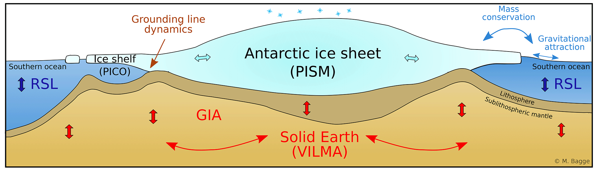
Figure 1 Schematics of coupled Parallel Ice Sheet Model (PISM)–Potsdam Ice-shelf Cavity mOdel (PICO)–VIscoelastic Lithosphere and MAntle model (VILMA) components. Bedrock topography, relative sea level (RSL) and ice thickness are exchanged between VILMA and PISM in predefined coupling time steps.

Geodetic and geophysical investigations of crustal uplift in the Amundsen Sea sector in West Antarctica (Barletta et al., 2018; Lloyd et al., 2020; Blank et al., 2021) postulate a laterally strongly varying viscoelastic Earth structure with mantle viscosities orders of magnitude lower than the global average. Hence, a low mantle viscosity implies much faster and, in the likely case of an also thinner lithosphere, a more localized (short-wavelength) response of the solid Earth to ice sheet retreat (van der Wal et al., 2015; Larour et al., 2019; Wan et al., 2022). Furthermore, geophysical investigations demand a clear dichotomy in the Earth structure between East and West Antarctica (Behrendt, 1999; Morelli and Danesi, 2004; Accardo et al., 2014; Lloyd et al., 2020; Powell et al., 2020). Also within West Antarctica a large degree of heterogeneity exists on length scales of 100 km (An et al., 2015; Ramirez et al., 2016; Heeszel et al., 2016), with hot spots of enhanced geothermal heat flux (Lough et al., 2013; Dziadek et al., 2021; Bredow et al., 2023).

The relative sea level (RSL), which is the water depth when positive or more precisely the vertical distance between the geoid and the bottom of the ocean, directly determines the grounding-line (GL) position of marine ice sheets via the flotation criterion. A global-mean (barystatic) sea level can be calculated from the global RSL change or by aggregating changes in ice sheet thickness and near-field RSL changes, based on the “volume above flotation” (Gregory et al., 2019; Goelzer et al., 2020; Adhikari et al., 2020). When ice sheets decay and the GL retreats, the viscoelastic solid Earth deformation reduces the water depth and hence induces a stabilizing negative feedback, which is additionally supported by near-field sea-level lowering in response to reduced gravitational attraction (Gomez et al., 2010, 2012, 2015; Coulon et al., 2021; Han et al., 2021).

As a side effect, the vertical bed displacement induces a bending of the elastic lithosphere and lateral viscous flow of mantle material, which is associated with the migration of a bulge with opposite RSL sign in the vicinity (Adhikari et al., 2014; Wan et al., 2022). Accordingly, local surface motion and slopes may change sign during lateral motion of the topographic bulge, which makes it difficult to isolate accelerating or inhibiting effects on the ice flow. During deglacial or interglacial periods, the “forebulge” subsidence is often associated with a mechanism termed “ocean syphoning” mainly in view of the Northern Hemisphere deglaciation (Mitrovica and Peltier, 1991; Mitrovica and Milne, 2002), which draws water from the far field and thereby contributes a far-field sea-level fall (Powell et al., 2021; Yousefi et al., 2022). The latitudinal extent of the forebulge region strongly depends on the lithosphere thickness. It can either be confined close to the coast and inner continental shelf for a thin lithosphere or reach offshore for thick lithospheres (Stocchi et al., 2013).

In grounded ice-sheet regions, where bedrock uplift directly affects the ice sheet's height, the surface climate becomes generally colder and drier (lapse-rate effect), which in turn affects the overall ice dynamics (Van den Berg et al., 2008; Konrad et al., 2014; Zeitz et al., 2022). Potentially, solid Earth feedbacks can slow down or even halt deglacial retreat, depending on the timescales of the viscoelastic deformation controlled by the structure of the solid Earth (Gomez et al., 2010; Konrad et al., 2015; Larour et al., 2019). In cooling phases with GL advance, i.e., during glaciation, coupled-model studies suggest a smaller glacial extent (and ice volume) than in standalone ice sheet models (forced with global-mean sea level), as self-gravitational attraction and local RSL changes dominate, associated with this negative (self-stabilizing) feedbacks of the RSL (Gomez et al., 2013; de Boer et al., 2014, 2017). This complex interplay of the solid Earth, sea level and ice dynamics has therefore played a major role during glacial cycles (Whitehouse et al., 2019) and is relevant for interpreting constraints on GIA in the periphery of the ice sheet, such as sea-level indicators and GPS uplift rates (Konrad et al., 2014).

A global sea-level low stand was reached during the Last Glacial Maximum (LGM) between 26 500 and 19 000 years before present (26.5–19 kyr BP; Clark et al., 2009). The rapid sea-level rise since the LGM due to the collapse of the Northern Hemisphere ice sheets likely contributed to the destabilization of the AIS, as iceberg-rafted debris records in deep-sea sediments suggest (Weber et al., 2014; Jones et al., 2022). Accordingly, this is reflected in an inter-hemispheric synchronicity of the large ice sheets' changes (Gomez et al., 2020).

There is growing evidence that during the Holocene period (the past 11 700 years) the solid Earth uplift in combination with ice rise formation may have caused the readvance of the Ross Sea GL to the present-day position after an initial phase of rapid deglaciation (Lingle and Clark, 1985; Kingslake et al., 2018; Johnson et al., 2022; Lowry et al., 2024), while in the Amundsen Sea GLs likely remained stable for the last 5500 years until recently (Braddock et al., 2022). The present-day state of the AIS, including its contemporary rates of change, characterizes its stability and the potential for sea-level rise in an increasingly warming climate (Joughin and Alley, 2011).

Ice sheet models have been coupled to GIA models with different levels of complexity (see the overview in Table 1 of Swierczek-Jereczek et al., 2024; de Boer et al., 2017; Whitehouse, 2018). The computationally efficient two-layer approach with an “elastic lithosphere and a relaxing asthenosphere” (ELRA) accounts for the vertical bedrock adjustment for one given relaxation time (Brotchie and Silvester, 1969; Le Meur and Huybrechts, 1996) and is widely used in ice sheet modeling or coupled Earth system modeling (Pollard and DeConto, 2012; DeConto and Pollard, 2016; Pattyn, 2017; Quiquet et al., 2018). The local response time and flexural rigidity can be also varied laterally (Coulon et al., 2021).

ELRA can be improved when the time-lagged mantle flow in the asthenosphere below an elastic thin plate is approximated by solving the corresponding biharmonic differential equation using fast Fourier transformation (Lingle and Clark, 1985; Bueler et al., 2007; Albrecht et al., 2020a; Book et al., 2022). In this “Lingle–Clark” (LC) bed deformation model, a wavelength-dependent response time spectrum replaces the single exponential-decay parameter of the ELRA approximation. Hence, only the uniform mantle viscosity and flexural rigidity (or elastic lithosphere thickness) are used as input parameters valid for the considered half-space.

In addition to the bedrock changes, global-mean sea-level anomalies are used as external forcing for ice sheet models to account for water depth changes at the GL (Goelzer et al., 2020). The LC model is limited to a certain region (e.g., Antarctica) and is unable to prescribe gravitational, globally self-consistent water-load changes or to account for feedbacks associated with polar motion due to GIA. The computationally inexpensive approach has been recently extended by considering lateral variations in the Earth structure and a regional sea-level change (Swierczek-Jereczek et al., 2024).

In order to account for both global and near-field spatial variability in relative sea-level change consistent with dynamic changes in ice sheet extent, coupled ice sheet–solid Earth models need to simultaneously solve the “sea-level equation” (Farrell and Clark, 1976), as realized in self-gravitating viscoelastic solid Earth models (SGVEMs; e.g., de Boer et al., 2014; Gomez et al., 2015, 2020; Konrad et al., 2015; Han et al., 2022). GIA models generally account for both solid Earth deformation and gravitational effects in combination with rotational effects in response to changes in the redistribution of ice and ocean masses (Milne and Mitrovica, 1996).

Most GIA models so far have computed changes in Earth deformation and geoid for a radially varying (depth dependent) 1D Earth structure using spherical harmonics (Whitehouse et al., 2012; Konrad et al., 2014, 2015; Pollard et al., 2017). In regions of a weak Earth structure, as for instance in West Antarctica, the observed uplift rates are not compatible with the response of a viscosity structure usually applied for Northern Hemisphere GIA in the range of 10²⁰–10²¹ Pa s and a lithosphere thickness of ≈ 100 km (Whitehouse, 2018; Ivins et al., 2023).

Since the 2000s, 3D viscoelastic Earth models have been developed (e.g., Martinec, 2000; Latychev et al., 2005; Wu et al., 2005; Zhong et al., 2022; Huang et al., 2023) and considered in a new generation of GIA models (e.g., Klemann et al., 2008; A et al., 2012; van der Wal et al., 2015; Nield et al., 2018; Bagge et al., 2021; Blank et al., 2021; Yousefi et al., 2022). Interactively coupled to ice sheet models, such 3D GIA models find significant differences in West Antarctic Ice Sheet (WAIS) evolution on glacial timescales compared to 1D GIA or standalone ice sheet models (Gomez et al., 2018; Han et al., 2022; Willeit et al., 2022; van Calcar et al., 2023; Swierczek-Jereczek et al., 2024). The underlying coupling methods all imply a similar iterative process to account for the unknown initial bed topography but differ with respect to the coupling time steps ranging from hundreds to thousands of years.

Here, we present a set of new simulations of AIS evolution over the last 246 000 years (i.e., two full glacial cycles) with the Parallel Ice Sheet Model (PISM) coupled to the VIscoelastic Lithosphere and MAntle model (VILMA) solving for GIA.

2 Methods

2.1 PISM

The Parallel Ice Sheet Model (here based on v1.2.2; see also “Code and data availability”; PISM User Manual, 2023) is an open-source 3D ice sheet model (Winkelmann et al., 2011; Khrulev et al., 2023) written in the C++ programming language. PISM has been previously applied in glacial-cycle simulations (e.g., Golledge et al., 2014; Sutter et al., 2019; Albrecht et al., 2020a, b) and can be easily coupled to other climate or Earth system model components (e.g., Kreuzer et al., 2021; Ziemen et al., 2019; Yang et al., 2022).

We here use a hybrid combination of two stress–balance approximations for the deformation of the ice, with the shallow-ice approximation–shallow-shelf approximation (SIA–SSA; Hindmarsh, 2004), which guarantees a smooth transition from vertical-shear-dominated flow in the interior via a sliding-dominated ice stream to fast plug flow in the floating ice shelves (Bueler and Brown, 2009) while neglecting higher-order modes of the flow. Driving stress at the GL is discretized using one-sided differences (Feldmann et al., 2014). The GL position simply results from a flotation condition, without additional flux conditions imposed (Reese et al., 2018c). Basal friction and basal melt are interpolated according to a linear subgrid interpolation scheme (Gladstone et al., 2010; Seroussi and Morlighem, 2018; Bradley and Hewitt, 2024). Thus, GL migration is reasonably well represented in PISM (compared to Stokes flow), even for a coarse resolution (Pattyn et al., 2013; Feldmann et al., 2014).

Ice deforms according to the Glen–Paterson–Budd–Lliboutry–Duval flow law with an exponent of n=3 (Lliboutry and Duval, 1985). PISM simulates the 3D polythermal enthalpy conservation for a given surface temperature and basal heat flux and thus captures melting and refreezing processes in temperate ice (Aschwanden and Blatter, 2009; Aschwanden et al., 2012). It is solved on a 3D grid with 81 vertical layers, with 20 m resolution at the base. The energy conservation scheme also accounts for the production of subglacial (and transportable) water (Bueler and van Pelt, 2015), which affects basal friction via the concept of a saturated and pressurized subglacial till. The till friction angle, which accounts for characteristics of the underlying substrate, has been optimized for present-day ice flow (Albrecht et al., 2020a). Depending on the resultant yield stress, this allows for grow-and-surge instability (Feldmann and Levermann, 2017; Bakker et al., 2017; Schannwell et al., 2023). Here we use the non-conserving hydrology model, where the till water content in each grid cell is balanced by basal melting and a constant drainage rate.

Ice shelf margins can evolve up to the edge of the continental shelf (here defined at 1800 m depth), constrained by a terminal-thickness criterion (>75 m). Iceberg formation from ice shelves is parameterized based on spreading rates (Levermann et al., 2012). Ice shelf melting is calculated using the Potsdam Ice-shelf Cavity mOdel (PICO) that considers basin-mean ocean properties on the continental shelf in front of the ice shelves and mimics the vertical overturning circulation in the ice shelf cavity (Reese et al., 2018a).

PISM comes with a generalized version of the Lingle–Clark bedrock deformation model (Bueler et al., 2007), assuming an elastic lithosphere, a resistant asthenosphere and a viscous half-space below (Whitehouse, 2018). The LC model is computationally efficient, with the default coupling time step being 10 years, but it does not account for regional sea-level variations due to gravitational attraction of the ice or of the deforming solid Earth.

A continental-scale representation of modern Antarctic bed and ice sheet topography is obtained from the Bedmap2 dataset (Fretwell et al., 2013). We simulate the entire Antarctic continent with 16 km grid resolution (381×381 grid points on a regular equidistant grid), compatible with the definition of the initMIP (initial state intercomparison exercise) and ISMIP6 (Ice Sheet Model Intercomparison Project for CMIP6; Coupled Model Intercomparison Project Phase 6) model intercomparison project (Nowicki et al., 2016, 2020). With an adaptive explicit time stepping of around 0.34±0.03 years, one glacial cycle (123 kyr) can be simulated within 1–2 d wall clock time with 64 CPU cores on a standard memory computing node at DKRZ (Deutsches Klimarechenzentrum, German Climate Computing Center; see https://docs.dkrz.de/doc/levante/configuration.html, last access: 5 June 2024; “AMD 7763” with 128 CPU cores in total, 256 GB main memory and a base clock of 2.45 GHz).

2.2 VILMA

The VIscoelastic Lithosphere and MAntle model (VILMA) solves the field equations for an incompressible self-gravitating viscoelastic sphere in the Lagrange domain, laterally in spherical harmonics, radially with finite elements and in time using an explicit time-differencing scheme assuming a Maxwell rheology as material law. Lateral variations in viscosity are considered to be shear energy perturbations, which are calculated on a Gauss–Legendre grid in the spatial domain and which are transformed back into the spectral domain at each time step (for details see Martinec, 2000). The code was benchmarked for a spherically symmetric Earth structure (Spada et al., 2011), i.e., for a 1D Earth structure, and was applied in studies accounting for lateral variations, i.e., for a 3D Earth structure (Klemann et al., 2008; Bagge et al., 2021). Furthermore, the effect of rotational feedback is accounted for (Martinec and Hagedoorn, 2014), following the discussion in Mitrovica et al. (2005).

The sea-level equation, describing the gravitationally consistent and mass-conserving redistribution of ice masses and ocean water in response to the deforming solid Earth (Farrell and Clark, 1976; Mitrovica and Milne, 2003; Kendall et al., 2006), is solved in the spatial domain (Hagedoorn et al., 2007) and was benchmarked in Martinec et al. (2018). Coastlines can freely migrate according to the local RSL. The loading effect of floating vs. grounded ice is accounted for. The GL position is determined by the flotation conditions and hence by densities of ice and ocean water (consistent with PISM). The GL migration is associated with a redistribution of water mass between ice sheets and the ocean, which can result in large non-uniform near-field RSL patterns (Mitrovica et al., 2001; Spada et al., 2013).

For the radial discretization, we chose Δz=5 km down to 420 km depth; followed below by Δz=10 km down to 670 km; and Δz=40 to 60 km down to the core–mantle boundary, where the parameterization of the elastic shear modulus and density structure follows the Preliminary Reference Earth Model (PREM; Dziewonski and Anderson, 1981). The interaction with the fluid core is considered a boundary condition, confining the solution domain to Earth's crust and mantle. The spectral resolution is set to a Legendre degree and order of 170, meaning that layers with lateral variations are discretized on a 256×512 (n128) grid corresponding to a wavelength of ∼120 km. The grid size is based on an alias-free condition, which defines the numbers of latitudinal Gauss–Legendre points to be larger than $\mathrm{3}/\mathrm{2}$ of the maximum Legendre degree considered (e.g., Martinec, 1989). We consider this sufficient due to the general low-pass response of Earth to surface loading and the spectral resolution of the considered tomographic model only up to a degree of 63 (Steinberger, 2016). Higher resolutions were tested in this project but did not show significant changes (see Sect. 3.1). The sea-level equation is solved in the spatial domain on a Gauss–Legendre grid but with a significantly higher resolution of 1024×2048 (n512) corresponding to a wavelength of ≈ 30 km.

In order to allow for restarts, the original Fortran 77 code was modularized and in main parts extended using Fortran 90 commands during the PalMod (Paleo Modelling) project (see the Acknowledgements), and OpenMP parallelization (OpenMP, 2012–2023) was implemented explicitly. In our coupled simulations, VILMA uses explicit time steps of 2.5 years in order to be able to solve also for very low mantle viscosities on the order of 10¹⁹ Pa s. Considering this setup, one glacial cycle (123 kyr) can be simulated within 19 h wall clock time with 64 CPU cores on a standard memory computing node (same as indicated for PISM).

2.3 PISM–VILMA coupling

PISM and VILMA are offline-coupled using a coupling time step that can be rather short and is only limited by the explicit time step chosen in VILMA and PISM. As a default, we apply a coupling time step of Δt=100 years, at which PISM and VILMA exchange data. The strategy, where ice load and relative sea level are exchanged (see below), was already applied in studies with an older version of VILMA coupled with the dynamic ice sheet models RIMBAY and PSUICE-3D (Konrad et al., 2014, 2015, respectively) and also in the Earth system model CLIMBER-X (Willeit et al., 2022), where the current VILMA version was coupled directly to the ice sheet model SICOPOLIS as a Fortran module. Here, for the first time, the 3D feature of VILMA is applied, whereas in the former studies only a 1D Earth was considered.

In a first step, PISM runs for the coupling interval (from t₀ to t₁), based on the initial bed elevation, which remains constant over the coupling time step Δt (see Fig. 2). Subsequently, VILMA integrates over the same interval (from t₀ to t₁) according to a global ice sheet load history, which combines ICE-6G_C (Peltier et al., 2015) north of 60° S and the PISM-simulated AIS changes south of 60° S, remapped to the VILMA grid. VILMA interpolates the ice sheet history between the snapshots at beginning and end of the coupling interval and provides the global change in RSL at predefined snapshots. The RSL at t₁ is (bilinearly) remapped back to the PISM grid.

Then, this process restarts for the next coupling interval (t₁ to t₂). PISM interprets the RSL change as negative vertical displacement of the bed elevation with respect to a reference surface elevation (geoid) or as change in water depth if the bed elevation has negative values. That means, the surface elevation of the ocean in the PISM simulations remains at z=0. With the adjusted bed topography (water depth), the ice sheet's GL can move directly due to the flotation criterion or indirectly due to induced ice-dynamical changes. These changes in the ice load are then passed to VILMA again, which simulates the same coupling time step (from t₁ to t₂), before PISM simulates for the next coupling interval.

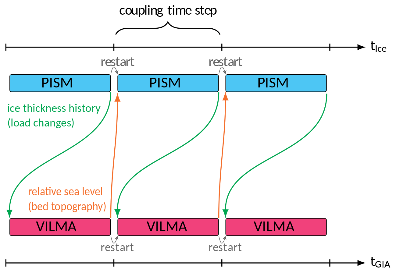
Figure 2 PISM–VILMA coupling scheme, adopted from Kreuzer et al. (2021).

In our coupling scheme, the PISM response always lags behind the VILMA step by one coupling step; i.e., RSL change from t_i−1 to t_i calculated in VILMA is only reflected in ice dynamics in PISM from t_i to t_i+1. The implied numerical error remains small if short coupling time steps are used (see the sensitivity to coupling time step in Sect. 3.1). We do not make use of (internal) iterations within a (longer) coupling time step as suggested, e.g., by van Calcar et al. (2023), even though this could be easily implemented in PISM–VILMA. Furthermore, we avoid extrapolation of sea-level and bed elevation changes to the next coupling interval as in Konrad et al. (2015), which principally can cause numerical instabilities. We also do not pass the subgrid information of GL interpolation, used in PISM for the basal friction, to VILMA. In case of GL migration, this could avoid ad hoc load changes from single grid cells. Our Python coupler (Albrecht, 2024b) uses CDO and NCO tools (CDO, 2024; NCO, 2003–2024) for remapping 2D RSL changes from the global Gauss–Legendre grid used in VILMA to the Antarctic Polar Stereographic (Maptiler, 2024) equidistant Cartesian grid used by PISM and, vice versa, Antarctic ice thickness from the PISM grid back to the global VILMA grid.

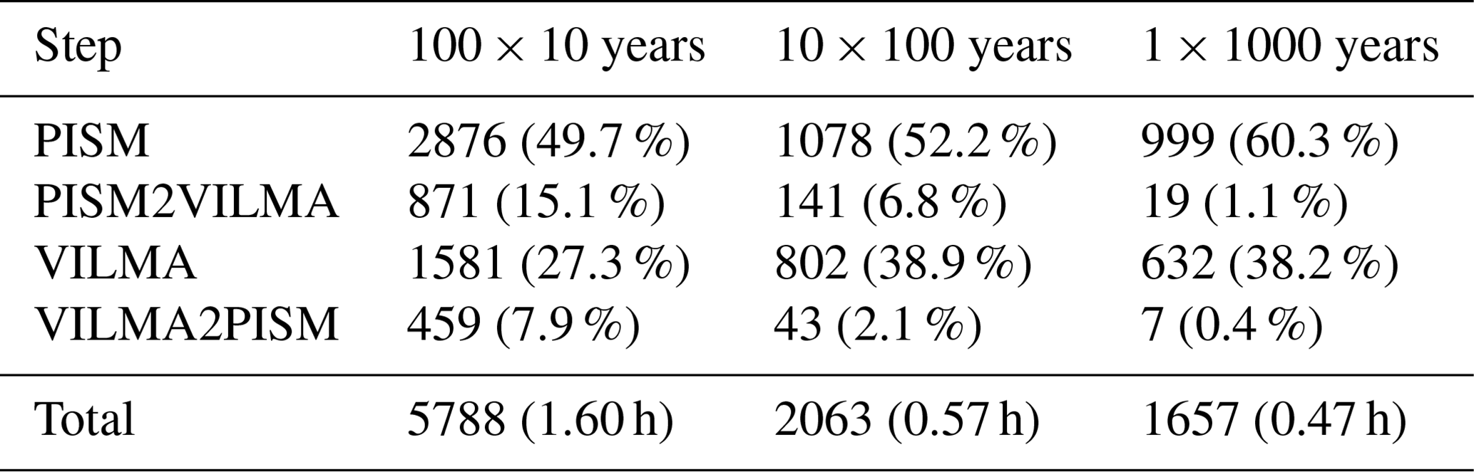
On a high-performance computing (HPC) system with a “slurm” batch queue system, we make use of the heterogeneous job support (SLURM, 2003–2024), which can simultaneously optimize for the OpenMP parallelization (OpenMP, 2012–2023) on a single compute node (in the case of VILMA and the Python coupler) and the MPI (Message Passing Interface) parallelization that can be utilized across multiple compute nodes (in the case of PISM). The remapping takes about 23 % of computational time for a 10-year coupling time step, 9 % for 100 years and only 1.5 % for 1000 years when using 3D Earth structures (see PISM2VILMA and VILMA2PISM in Table 1). The total computation time for simulating 1 kyr on a standard memory computing node (128 cores in total; see details in Sect. 2.1) is about 25 min for the 1000-year coupling time step (25 CPUh, CPU hours), 30 min for 100 years (35 CPUh) and 100 min for 10 years (100 CPUh) when using 64 CPU cores for VILMA, PISM and the remapping. Considering only 1D (radial) Earth structures in VILMA brings a speedup by a factor of 5 for the VILMA step and hence an almost 50 % speedup in the coupled-model performance, for coupling time steps of 100 years.

For comparison, van Calcar et al. (2023) used a 3D GIA finite-element model with 16 CPU cores to simulate the last glacial cycle, with coupling time steps between 5000 and 500 years, 40 km resolution in the ice sheet model, and between 30 and 200 km in the GIA model, showing a performance of 16 CPUh for 1000 model years. However, when internal iterations were considered, the coupled model system required about 120 CPUh for 1000 model years.

Table 1 Mean wall clock time for PISM–VILMA steps in seconds (and percent) for a 1 kyr simulation for the reference 3D Earth structure with 64 CPU cores and different coupling time steps, run on Levante (DKRZ). All three coupled simulations used the reference spatial resolution of n512 for the sea-level equation in VILMA, n128 for the viscoelastic deformation in VILMA and 16 km for PISM in the Antarctic domain.

In order to account for (long) memory effects of the AIS to the climate history, we run the coupled simulation for two full glacial cycles (246 kyr; see Fig. 3a), with the Northern Hemisphere described by the ICE-6G_C reconstruction (available for the last 122 kyr, repeated for the penultimate glacial cycle with a time shift by 124 kyr and concatenated at the Last Interglacial), similar to Han et al. (2022). For consistency, the climatic and ocean forcings are applied as described in previous PISM standalone simulations (Albrecht et al., 2020a), which have been coupled to the LC bed deformation model (Bueler et al., 2007). In order to support an earlier deglaciation around 15 kyr BP (see Fig. 3b) providing a better match with paleoproxies (Briggs and Tarasov, 2013; Albrecht et al., 2020b), PISM parameters were slightly adjusted in this study (e.g., till water drainage rate or precipitation scaling). Simulations are run until the year 1950 (corresponding to 0 kyr BP) such that the recent anthropogenic warming is ignored in the ice-core-reconstruction-based climate forcing (here a combination of European Project for Ice Coring in Antarctica (EPICA) Dome C and WAIS Divide ice core; see Albrecht et al., 2020a).

For the initial global bed topography we apply the present-day ETOPO1 bathymetry (Amante and Eakins, 2009), updated with Bedmap2 (Fretwell et al., 2013) in the Antarctic sector. As the initial bed topography of the simulation (at 246 kyr BP) is not known a priori, we iterate several times over the period of two glacial cycles (Kendall et al., 2005; van Calcar et al., 2023) and successively correct for the initial bed topography according to the mismatch of the present-day bed topography to observations from Bedmap2 of the previous iteration (compare Figs. 3 and 4). Ideally, the present-day RSL subtracted from the initial bed topography should converge to the present-day topography. In the first iteration, the present-day RSL is underestimated by up to 100 m in East Antarctica (bedrock too high) and overestimated by up to 100 m in West Antarctica (Fig. 4a). As a measure of the mismatch we use the root mean square error (RMSE) over the Antarctic computational domain. Generally, the RMSE reduces with each iteration by a factor of 0.2–0.4 (see Fig. 3c). We stop iterating when the RMSE falls below the acceptance level of 10 m (dotted line). This iterative procedure aims at minimizing deviations from the present-day bed topography, but we also find convergence of the present-day Antarctic ice volume against observations (Fig. 3b); nevertheless, in some regions the misfit in ice thickness remains comparably high (Fig. 4g–l). In order to convert Antarctic ice volume change into more practical units for better comparison, we here use the approach of volume above flotation with corrections for the density and in regions grounded below sea level (Adhikari et al., 2020, Eq. 10). We apply this approach to the projected regional ice model domain using cell-area weights and a constant ocean area of 362.5×10⁶ km². Compared to an ice-free state with present-day bed topography, this conversion provides a global-mean estimate of the “sea-level rise potential” (SLRP) in units of meters of sea-level equivalent (m SLE). As vertical land motion is already included in our RSL variable, we do not explicitly account for the “water-expulsion effect” in the conversion (Goelzer et al., 2020; Pan et al., 2021).

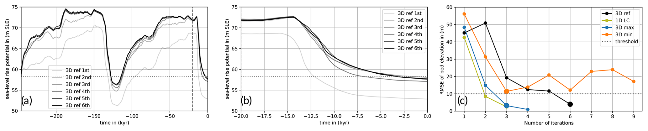
Figure 3 Sea-level rise potential in a coupled PISM–VILMA simulation (a) over the last 246 kyr and (b) over the last 20 kyr, showing convergence for six subsequent iterations with a reference 3D Earth structure (3D ref) at an n128 resolution and n512 resolution for the sea-level equation. In each iteration the initial bed topography is adjusted such that the misfit of present-day bed topography according to VILMA is minimized. (c) Root mean square error in present-day bed topography anomalies in subsequent iterations for four different Earth structures (see Sects. 2.4 and 3.3). Big markers indicate the last iteration selected for further comparison.

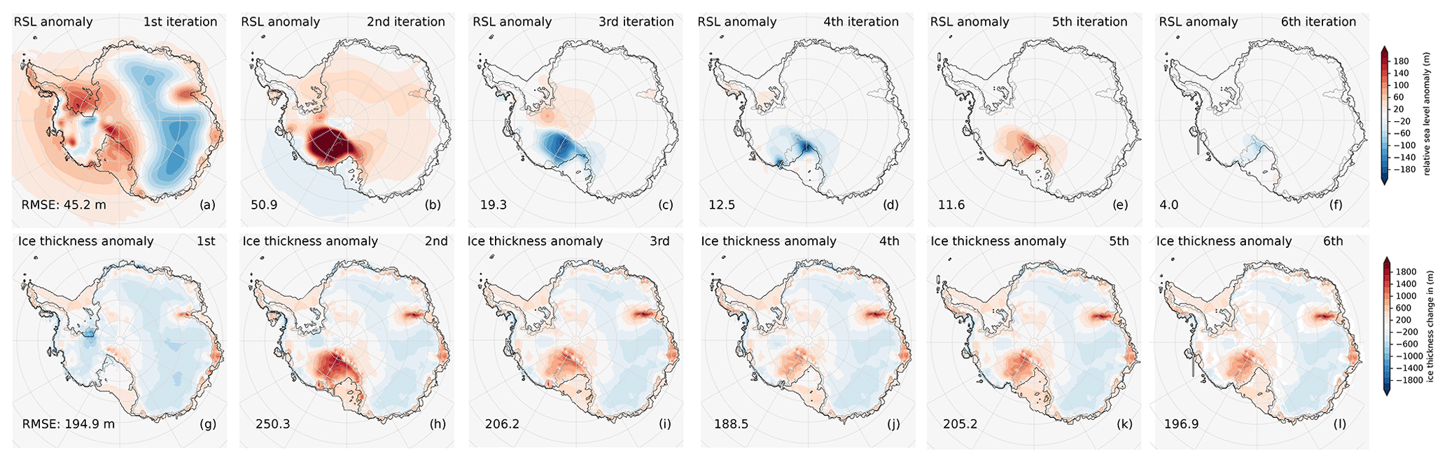
Figure 4 Anomalies of RSL (VILMA) and ice thickness (PISM) at present day compared to Bedmap2 bed elevation and ice thickness observations (Fretwell et al., 2013), for six iterations of coupled glacial-cycle simulations with a reference 3D Earth structure (3D ref; see Sect. 2.4), converging from 46 m RMSE to about 4 m RMSE for the RSL anomaly (negative bed topography anomaly; cf. black points in Fig. 3c). This iterative procedure does not optimize for the present-day ice thickness. The iterations show a convergence with an alternating sign in the mean RSL anomaly, particularly in the Siple Coast region in the Ross Sea sector. Black lines indicate modeled GL and ice shelf extent; grey is the observed GL.

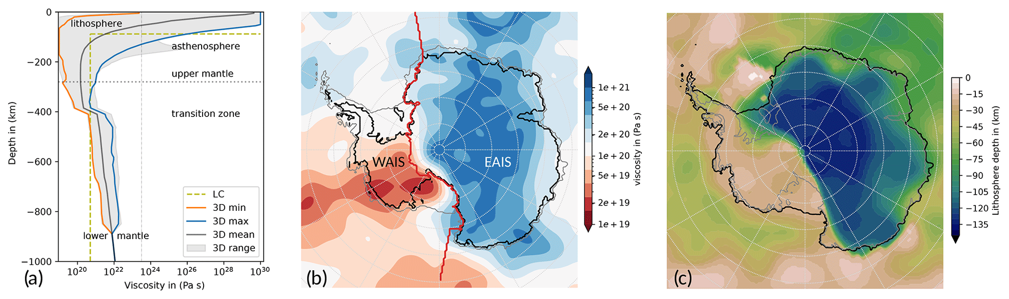
Figure 5 VILMA Earth structure. (a) Vertical profiles of viscosity down to 1000 km depth for 3D Earth structures, with a global logarithmic mean and range (grey), the Antarctica-wide range (between orange and blue defining 3D min and 3D max, respectively), and the two-layer profile as used in the Lingle–Clark model (olive). (b) 3D ref at 280 km depth (horizontally dotted line in a, showing a lateral variability of 2 orders of magnitude, 10¹⁹–10²¹ Pa s). Present-day grounding line and calving front (Bedmap2 contours from Fretwell et al., 2013, in grey and black, respectively) and Zwally et al. (2012) drainage basin divide (red) between WAIS (basins 2–17) and East Antarctica (basins 18–27 and 1). (c) Lithosphere depth defined by a 10^23.5 Pa s threshold (vertical dashed line in a, showing a thin lithosphere of <50 km in West Antarctica and a thick lithosphere exceeding 130 km in East Antarctica).

2.4 Solid Earth structures

Between the West and East Antarctic plates, differences in the upper-mantle viscosity, here shown at 280 km depth, can exceed 2 orders of magnitude (Fig. 5b). Based on seismic tomography models and geodynamical constraints, a dataset for the 3D Earth structure (including the lithosphere thickness) has been optimized such that the VILMA response minimizes the misfit to a global compilation of RSL records (Bagge et al., 2021). According to their global investigation the 3D viscosity is bounded below by 10¹⁹ Pa s, which keeps integration time manageable for glacial-cycle simulations. We do not modify the 3D Earth structure in view of geodetic inferences as these discuss recent load changes in specific Antarctic regions (e.g., Nield et al., 2014; Barletta et al., 2018), which are not the scope of this study. In the following we refer to the Class-I type (“v_0.4_s16”) as our reference 3D Earth structure (“3D ref”).

In order to test for the effects of low and high viscosities on the ice sheet dynamics and to investigate possible feedbacks, we define end-member Earth structures of the laterally varying reference 3D Earth structure, 3D ref. The “3D min” and the “3D max” cases take the minimum and maximum of 3D ref over the Antarctic region south of 60° S at each depth interval (see Fig. 5a), respectively. The inferred minimum or maximum defines a laterally uniform 1D Earth structure within the Antarctic region, while north of 60° S we consider the original 3D ref structure, as we want to avoid far-field effects induced by changes in the Northern Hemisphere Earth structure. This implies a very thin lithosphere thickness of only a few kilometers and upper-mantle viscosities down to 10¹⁹ Pa s in the 3D min case for Antarctica, while in the 3D max case, the lithosphere thickness is around 130 km and upper-mantle viscosities remain larger than 4×10²⁰ Pa s for all depth intervals (Fig. 5c).

3 Results

3.1 Sensitivity of AIS deglaciation to spatial resolution and the coupling time step

The coupling time step is an important parameter in a coupled model system. Although PISM responds to changes in RSL from VILMA in the previous time step, the coupling time step should be short enough to avoid delay effects. However, computational costs for the remapping of the spatial fields and the initialization of each of the model steps are incurred at each coupling time step (cf. Table 1). A reasonable coupling time step therefore balances costs and accuracy.

We evaluate the sensitivity of the coupled simulations to coupling time steps Δt of 1000, 100 and 10 years by comparing the deglacial response of the AIS over the last 20 kyr. In all three cases we find a similar SLRP during the LGM (in our simulations around 15 kyr BP) of around 72.5 m SLE, which is about 14 m SLE above the present-day level (see Fig. 6a). At the onset of deglaciation, around 14 kyr BP, we find small discontinuities in the response for the largest coupling time step (blue lines), as PISM responds to changes in bed topography that remain constant for the 1000-year interval, while the far-field RSL changes dramatically during “meltwater pulse 1A” (MWP-1a). In fact, this is partly a consequence of the diagnostic calculation of the SLRP, since changes in bed elevation also affect the flotation height and hence potential sea-level contributions. The solid blue line would be much smoother if total ice mass or grounded-ice volume over time were shown. Interestingly, compared to Δt≤100 years, we find during the Holocene until the present day a slightly smaller SLRP (by about 1 m SLE) for Δt=1000 years. In the case of a linear extrapolation of the RSL change rate in the PISM step for this Δt (dashed blue line in Fig. 6a), we find a similar effect during deglaciation, with slightly earlier deglaciation than without extrapolation. Comparing the ice sheet response for Δt=100 years and 10 years, we see only little differences for the given spatial resolution of n512/n128 in VILMA and 16 km in PISM, which we interpret as “convergence”. It should be noted that the coupled system is highly non-linear with a high sensitivity to initial conditions. Convergence should be considered with respect to a certain range of internal variability (Albrecht et al., 2020a).

As total computational costs per modeled 1000 years increase by about 20 % between 1000 years and 100 years but by about 65 % between 100 years and 10 years, we choose Δt=100 years as the default coupling time step for further experiments.

A recent study on time stepping and RSL precision (Han et al., 2022) with the coupled ice sheet–sea-level model system of Gomez et al. (2013, 2020) suggests coupling time steps of at least 200 years, while a previous coupled-model study with coarser spatial resolution claimed that 1000 years would be sufficient (de Boer et al., 2014). Coupling time steps of 500 years are shown to yield accurate results when using internal iterations and linear interpolation over the coupling time step (van Calcar et al., 2023). Idealized experiments performed with a coupled-model framework with VILMA led to the choice of 50 years (Konrad et al., 2015). In fact, an optimal temporal resolution is highly linked to the spatial resolution and the involved Earth structure.

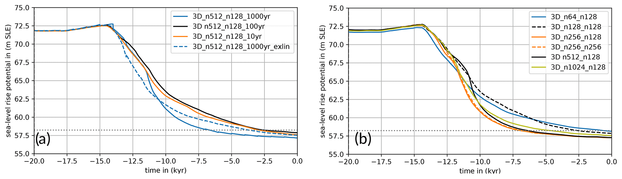
Figure 6 Sea-level rise potential from Antarctica over the last 20 kyr for different coupling time steps and different spatial resolutions. (a) Default coupling time step is 100 years (black). Higher temporal resolution of 10 years is shown in orange. Lower temporal resolution of 1000 years is shown in blue, with linear extrapolation (“exlin”) of the RSL change rate as a dashed blue line. Here, all simulations were restarted from the same restart state at 20 kyr BP (3D ref, sixth iteration with default spatial resolution). Shown time series have a resolution of 10 years. (b) Reference spatial resolution is n512 for the sea-level equation in VILMA, n128 for the viscoelastic deformations and 16 km in PISM (black). Higher spatial resolution for the sea-level equation is shown in olive (n1024); coarser resolution is shown in blue (n64), as a dashed black line (n128) and in orange (n256). As a dashed orange line, the resolution for the viscoelastic deformations has also been increased to n256. All simulations have been initiated from the same initial state at 246 kyr BP (fourth iteration). The coupling time step and temporal resolution of the plotted time series is 100 years. PISM resolution has not been varied here.

There are interactive processes between ice sheets, the ocean and the solid Earth that need sufficient spatial resolution to be adequately resolved, in particular in the grounding zones of marine ice sheets. The default spatial resolution in our coupled simulations is 16 km in the AIS and 0.2° for the global sea-level equation (n512), which corresponds to 20 km in latitude and to about 6 km in longitude at 71° S. The viscoelastic deformation is resolved with 0.7° (n128), which corresponds to about 78 km in latitude and 25 km in longitude at 71° S. A doubling in the viscoelastic resolution (n256) has only minor effects on the AIS deglaciation (see orange lines in Fig. 6b). A coarser spatial resolution in the sea-level equation, however, delays deglaciation during the Holocene (solid blue and dashed black lines for n64 and n128, respectively), with a SLRP difference of up to 2 m SLE compared to the reference resolution. These differences mainly result from RSL anomalies in the Ross Sea section (Fig. S1 in the Supplement). Only small differences in SLRP are found at around 11 kyr BP for even higher spatial resolutions (cf. olive and black lines for n1024 and n512, respectively). The resolution of the ice sheet model has not been varied here, as this would require a new ensemble of simulations to constrain model parameters, as well as for the complex geometry of the AIS, since some parameters are resolution dependent (Albrecht et al., 2020a, b).

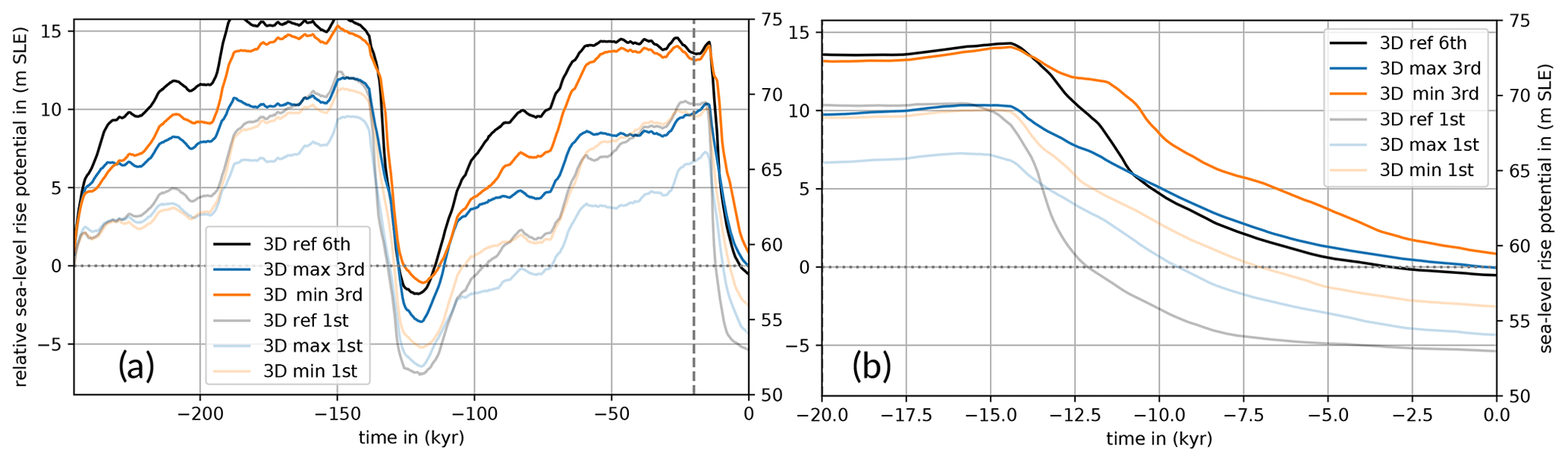
Figure 7 Sea-level potential rise from Antarctica over the last 246 kyr and over the last 20 kyr for different Earth structures. Blue and orange lines show the response of the AIS in the cases of 3D min and 3D max (cf. Fig. 5a), meaning respective 1D Earth structures south of 60° S and 3D further north. Black lines indicate the SLRP response to 3D ref, i.e., 3D also for Antarctica. Transparent lines show the first-iteration results with the same initial topography; dotted horizontal line is the present-day observation from Bedmap2 (Fretwell et al., 2013).

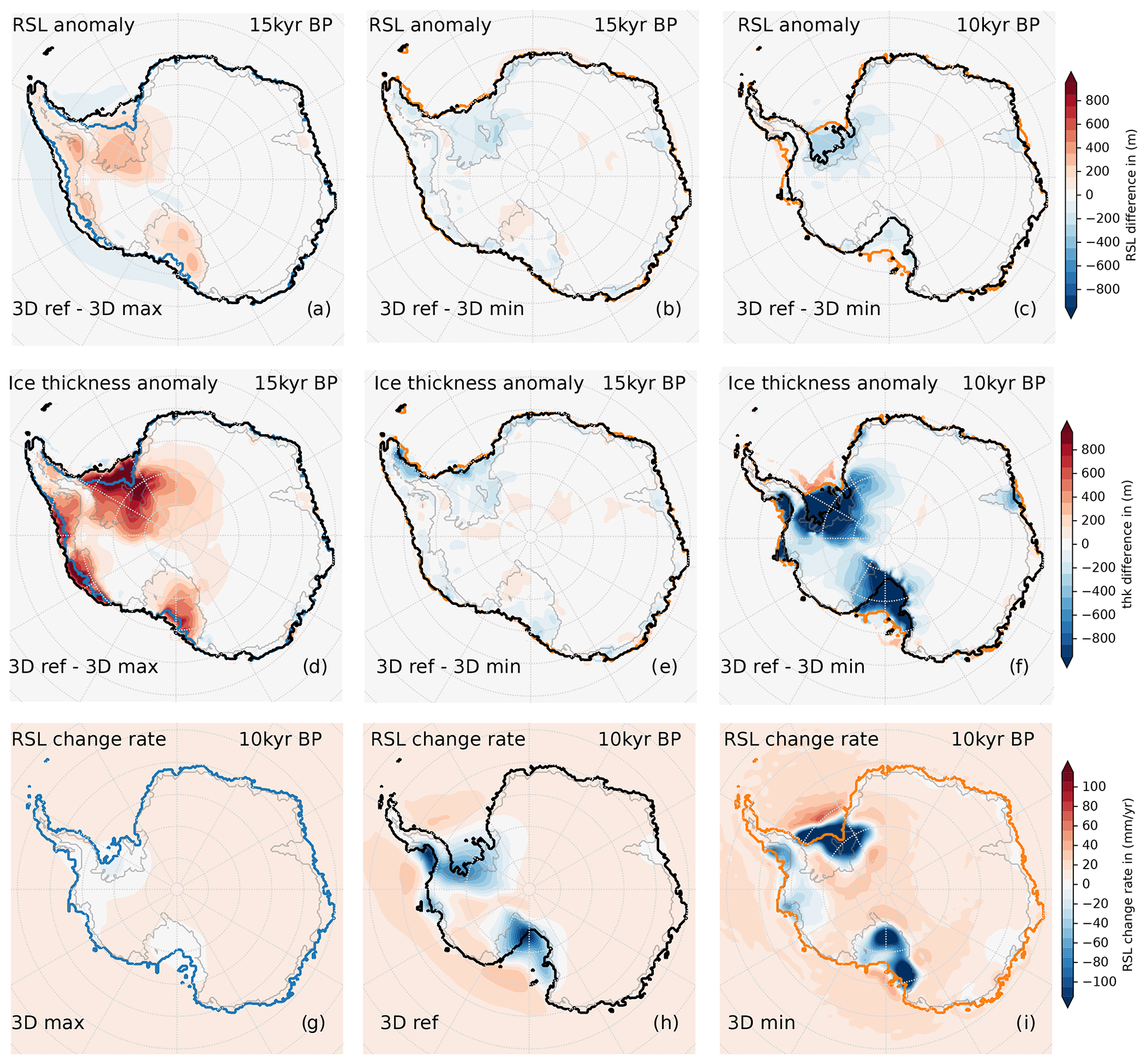
Figure 8 Difference in (a–c) relative sea level and (d–f) ice thickness for different Earth structures at 15 and 10 kyr BP and RSL change rates at 10 kyr BP for (g–i) the different Earth structures. The modeled GL positions due to the different Earth structures are shown as contour lines for 3D min (orange), 3D max (blue) and 3D ref (black) and at present day (grey).

3.2 AIS buildup and deglaciation within the bounds of a reference 3D Earth structure

The reference 3D Earth structure (3D ref) discussed in Bagge et al. (2021) implies a large range of lithosphere thickness and mantle viscosity in key regions of the AIS. In order to evaluate effects of lateral variations in the underlying Earth structure on ice dynamics, we discuss changes in the grounded AIS area (GL extent) and its SLRP over the last 246 kyr.

First, we consider the lower bound of 3D ref, i.e., 3D min (Fig. 5a). In our coupled simulations with 3D min (third iteration), the AIS holds about 14 m SLE more SLRP during the LGM (here at 15 kyr BP) than observed at present day. This corresponds to a maximum LGM grounded-ice area of 15.9×10⁶ km² (Fig. 7b) and a total ice mass of 31.2×10⁶ Gt, respectively. For the highly viscous 3D max, the SLRP during the LGM reaches only 10 m SLE above the present day, corresponding to 28.9×10⁶ Gt and 15.1×10⁶ km² grounded ice-sheet area. In both cases, the WAIS contributes 2–3 times more ice to the rising sea level since the LGM than the East Antarctic Ice Sheet (EAIS) (Fig. S4a). The largest differences in ice sheet response between 3D min and 3D max can be detected in the Ross and Ronne Ice Shelf basins and in the Bellingshausen and Amundsen Sea, where for 3D min locally the RSL is up to 500 m higher (and hence the underlying bedrock is deeper), leading to more extended and more than 1000 m thicker grounded ice (cf. Figs. 8a and d and 8b and e, as 3D min and 3D ref have a similar LGM extent). In Sect. 4, we will discuss this additional feedback mechanism that can explain enhanced GL advance during the LGM for weak Earth structures.

In the first iteration, without corrected initial bed topography, we find already similar differences in AIS evolution over time for the different Earth structures but generally 3–4 m SLE lower SLRP (transparent lines in Fig. 7a, b) and smaller grounded ice-sheet areas (transparent lines in Fig. S2b) than for the last iteration. During the iterations, bed topography and SLRP converge at present day towards their observed values (Fig. 3c). However, modeled grounding lines at present day tend to slightly expand the observed grounded-ice extent (solid and dotted lines in Fig. S2b).

The onset of deglaciation in our simulations occurs after MWP-1a around 14.5 kyr BP (Peltier, 2005), with a global-mean sea-level rise of about 20 m during the following 350 years (which corresponds to a mean rate of 50 mm yr⁻¹; see Fig. S4b, c). This far-field effect, mainly in response to the Northern Hemisphere ice sheet losses (ICE-6G_C), reduces to about 10 mm yr⁻¹ between 14 and 7 kyr BP (in total around 55 m of global-mean sea-level change) and partly compensates for near-field sea-level drop in Antarctica, e.g., by viscoelastic bedrock uplift or gravitational attraction (see Fig. 8g, i at 10 kyr BP; cf. Gomez et al., 2020). During the deglaciation until the present day we find a slightly slower decline, both in SLRP and grounded-ice area for 3D min compared to 3D max (Figs. 7b and S2b). As their SLRP values differ by around 4 m SLE during the LGM, they provide different initial conditions at the onset of deglaciation. Grounding-line retreat and ice sheet thinning (leading to ice shelf formation) can be slowed down if the isostatic rebound responds to these changes on rather short timescales. For 3D min, RSL change rates are in fact much higher than for 3D max, in West Antarctica reaching up to −500 mm yr⁻¹ instead of −20 mm yr⁻¹, while in the far field, the RSL rises by about 10 mm yr⁻¹, indicated by light-orange shading on the corners of the maps in Figs. 8g, i and S4c, d. This quick and rather localized response (e.g., Wan et al., 2022) defines a negative and hence stabilizing feedback on GL retreat (Gomez et al., 2010, 2012). For 3D min, rates of RSL change and grounded-ice area retreat remain almost constant at this comparably low level until the present day. The viscoelastic rebound can take several millennia for 3D max, and, in consequence, the stabilizing effect can be significantly delayed and is active on a larger lateral extent. Over the last 3 kyr the AIS even tends to readvance slightly (Fig. S2b), as suggested in earlier studies (with PISM–LC) for rather high mantle viscosities of 5×10²⁰ Pa s (Kingslake et al., 2018).

The reference 3D Earth structure 3D ref accounts for both the weak Earth structure in West Antarctica and the higher mantle viscosities and thicker lithosphere in East Antarctica (Fig. 5b, c). The corresponding response of the AIS for 3D ref shows an SLRP (72.5 m SLE) and ice sheet area (15.8×10⁶ km²) during the LGM similar to that for 3D min (Figs. 7b and S2b, black and orange contours, respectively). The largest differences in the ice loads, compared to 3D max, are located in the West Antarctic region, where a rather low mantle viscosity and a thin lithosphere are dominant (Fig. 8a, d). The additional ice load causes further subsidence of the bedrock underneath, by up to 200 m more than for 3D max (Fig. S6), while in the adjacent coastal region, the sea floor becomes about 50 m shallower than for 3D max (Fig. 8a, light-blue shading). This feature is called forebulge and results from lateral transport of displaced mantle material and the flexure of the lithosphere. For 3D ref, ice loss rates can reach 1500 Gt yr⁻¹ in the first millennia after the onset of deglaciation (Fig. S4f). This is slightly higher and also earlier than for 3D min and generally higher than for 3D max (<500 Gt yr⁻¹). Maximum bedrock uplift rates with up to 200 mm yr⁻¹ are reached for the low-viscosity response in West Antarctica (Fig. 8h), while maximum uplift rates below 50 mm yr⁻¹ are associated with higher viscosities and a thicker lithosphere in East Antarctica (Figs. S4d and Video S1; Albrecht, 2023).

At present day, the SLRP, grounded-ice area and ice mass for 3D ref (sixth iteration) converges at 57.7 m SLE, 13×10⁶ km² and 24.6×10⁶ Gt, respectively, which is close to observations (in our diagnostic: 58.2 m SLE, 12.6×10⁶ km² and 24.3×10⁶ Gt; dotted lines in Figs. 7a and b, S2b, and S3b).

Counterintuitively, the SLRP response for 3D ref does not show a trajectory completely in between the two end-members, 3D max and 3D min. Yet, the coupled simulations reveal that in glacial periods of GL advance the SLRP trajectory evolves in a way similar to the trajectory for the weak Earth structure (3D min), while in deglacial periods of GL retreat the SLRP from the AIS responds in a way similar to the trajectory for the stiffer Earth structure (3D max). The similarity of 3D max and 3D ref responses during deglaciation is even more pronounced for similar LGM ice sheet conditions (ice sheet history until 20 kyr BP prescribed as in 3D ref; see the dashed blue line in Fig. S2a).

One important aspect to consider when using ice volume above flotation as a metric is that the bed elevation changes imply changes in the grounded-ice area and the converted potential sea-level contributions. Other metrics, e.g., the total ice mass, are independent of bed elevation or sea-level changes. Figure S3b shows that the differences in total ice mass evolution between 3D ref and 3D min are reduced during glacial maxima. Another aspect is a cumulative effect of the performed iterations, with shifted initial bed elevations depending on the present-day anomalies and hence also on the LGM state and the rate of deglaciation. In the first iteration all simulations are initiated with the same bed elevation and ice thickness distribution such that differences over time can be purely attributed to effects resultant from the different Earth structures (see transparent lines in Figs. 7a, S2b and S3b). With every iteration the differences in ice volumes and ice masses become larger for different Earth structures, in particular during phases of glacial buildup.

3.3 Comparison to glacial-cycle simulations with the PISM–LC model

In order to discuss the impact of the more complete GIA model considered in the PISM–VILMA simulations, we run coupled PISM–LC simulations with the global-mean sea-level (GMSL) change derived from a coupled simulation with a 1D Earth structure (described in the next paragraph). The resultant GMSL time series is similar to the one obtained with 3D ref, as well as to the global-mean ICE-6G_C obtained with the “VM5a” Earth structure (90 km lithosphere and 500 km thick upper mantle with 5×10²⁰ Pa s), as in all cases the same ice thickness history for the Northern Hemisphere is used (cf. Figs. 9a and S4b). Note that in the PISM–LC coupling the change in GMSL is interpreted as a change in sea surface height. For the same PISM parameters and climatic forcing as in the PISM–VILMA simulations, we find after three iterations with PISM–LC a much lower SLRP from Antarctica, with 59 m SLE during the LGM (13.5 m SLE lower than for 3D ref) and 56.5 m SLE at present day (1 m SLE lower than for 3D ref) (olive vs. black in Fig. 9b). Differences in LGM ice volume mainly result from a smaller GL extent during the LGM, especially in the Weddell Sea sector (Fig. S6). The PISM–LC results provide an estimate of the influence of GIA, although the inferred LGM ice volume in Antarctica does not seem realistic. Previous model simulations, some of them scored against different paleo-climate records, suggest that the (uncorrected) SLRP during the LGM in Antarctica was around 10 m SLE larger than at present day (cf. Fig. S3a and see Fig. 11b in Albrecht et al., 2020b). For a slightly adjusted PISM parameter combination, a larger glacial-ice-sheet extent can be reproduced (Kingslake et al., 2018; Albrecht et al., 2020a).

If PISM–VILMA is run, analogous to PISM–LC, with a globally constant viscosity for the whole mantle of 5×10²⁰ Pa s and a lithosphere thickness of 88 km (see Fig. 5a), we obtain lower SLRP from Antarctica than for 3D ref (purple vs. black in Fig. 9b). In particular during glacial buildup the SLRP is about 10 m SLE smaller, whereas during the LGM it is around 6.5 m SLE smaller (Fig. 9a, b). This is likely a consequence of the thicker lithosphere and the higher mantle viscosity in large parts of West Antarctica, represented in the simpler Earth model. Compared to the response from the PISM–LC simulations (olive line in Fig. 9b), the SLRP during the LGM is about 7 m SLE larger, likely a consequence of potentially stabilizing gravitational and rotational effects accounted for in VILMA. Regardless of the significant differences during glaciated periods, the present-day (and Last Interglacial) SLRP values differ by less than 1 m SLE in these simulations (Fig. 9b), as the iterative procedure minimizes the present-day misfit in bed topography.

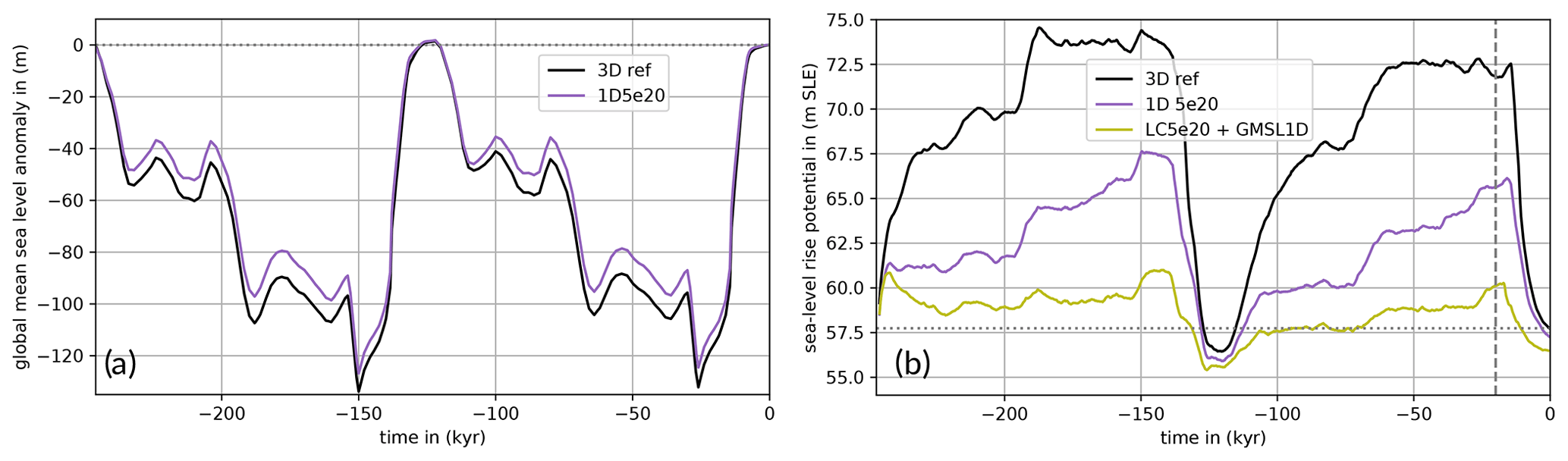
Figure 9 Comparison of (a) global-mean RSL and (b) SLRP from Antarctica over last 246 kyr for Earth models of different complexities. Olive for the Lingle–Clark bed deformation model with a 100-year coupling time step, upper-mantle viscosity of 5×10²⁰ Pa s (“LC 5e20”) and 88 km lithosphere thickness (5×10²⁴ Nm flexural rigidity), suggesting a loss of about 3 m SLE in SLRP since the LGM. Purple for the coupled PISM–VILMA model with a 100-year coupling time step, a 1D Earth structure with an 88 km thick elastic lithosphere and 5×10²⁰ Pa s viscosity in the mantle below (“1D 5e20”). This simulation also solves for the sea-level equation, yielding a 7 m SLE larger contribution since the LGM. The global mean of the sea level is used as forcing for the simulation with the LC model (“GMSL1D”). In black, the AIS response to the reference 3D Earth structure 3D ref is shown with more than 14 m SLE change in SLRP since the LGM.

3.4 Far-field and near-field RSL effects on Antarctic deglaciation

In this section, we focus on the dynamics of the AIS in response to the Northern Hemisphere ice sheet's decay. We will provide an estimate of the far-field and near-field components of RSL change since the LGM and compare our coupled-simulation results with previous experiments in literature. Gomez et al. (2020) use a coupled ice sheet–GIA model that incorporates a global 1D (radially varying) viscoelastic mantle structure with four layers: a 50 km thick lithosphere, a 150 km thick low-viscosity zone of 10¹⁹ Pa s (representative of the weak Earth structure beneath the WAIS), an upper-mantle viscosity of 2×10²⁰ Pa s and a lower-mantle viscosity of 3×10²¹ Pa s below 670 km depth (see Fig. S7a). Like in our coupled simulations, Gomez et al. (2020) prescribe the Northern Hemisphere ice sheet history (ICE-5G; see anomaly during the LGM in Fig. 10a), while the AIS evolution is simulated with a dynamic ice sheet model (PSU-ISM with 20 km resolution). Sea-level calculations are performed up to a spherical harmonic degree of 512 and coupled every 200 years. Key differences are that PISM–VILMA uses a global 3D Earth structure and iterations are performed over the last two glacial cycles (246 kyr instead of starting at 40 kyr BP). On the one hand we have to acknowledge a long memory in the ice sheet's thermal state on the order of 100 kyr (Briggs et al., 2013; Albrecht et al., 2020a). On the other hand the LGM ice volume depends on the previous glacial buildup and the rate of deglaciation depends on the LGM ice volume. The potential sea-level contribution from the AIS since the LGM (here at 21 kyr BP) is considerably larger in our simulations (13 m SLE instead of 5 m SLE). In their coupled-model setup, the simulated AIS volume changes since the LGM suggest a rather low sensitivity to different radial 1D and 3D Earth structures (Pollard et al., 2017; Gomez et al., 2018).

In our coupled PISM–VILMA simulations, maximum LGM sea-level fall of more than 400 m in the West Antarctic Ross and Weddell embayments is much larger than the 150 m found in Gomez et al. (2020), although the spatial pattern of RSL change is similar. The barystatic mean sea-level change since the LGM we find to be 120 m. If we prescribe the present-day AIS configuration through the GIA simulation, we can estimate the far-field RSL pattern in response to Northern Hemisphere ice sheet loss since the LGM. It has a clear imprint of Earth rotational effects, with 75 m in East Antarctica and up to 125 m in West Antarctica (Fig. 10c), and is in agreement with Gomez et al. (2020). Subtracting the far-field RSL pattern provides a first-order estimate of the near-field GIA effects, mainly the deformational and gravitational GIA components. Accordingly, bedrock elevation in the interior of West Antarctica has been uplifted since the LGM by up to 540 m and in East Antarctica by less than 100 m (see Fig. 10d). At the edge of the continental shelf, a peripheral forebulge of an opposite sign developed, with up to 85 m vertical bedrock displacement since the LGM. This feature is presumably smaller and hence not visible in the corresponding plots of Gomez et al. (2020), likely as a result of the much smaller deglacial AIS losses.

To test the impact of sea-level forcing, we have also performed coupled PISM–VILMA simulations with the Northern Hemisphere ice history fixed at its stage at 40 kyr BP, and hence a continuing far-field RSL of around 100 m below its present-day value. We found that the AIS remains almost at its LGM state until the present day (Fig. S7), confirming the importance of sea level in triggering deglacial changes as already stated in Albrecht et al. (2020a). In a similar experiment, Gomez et al. (2020) find a delayed and less pronounced deglacial GL retreat in Antarctica.

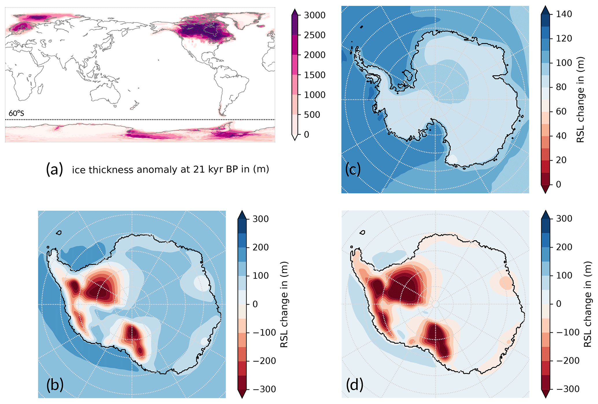
Figure 10 Far-field and near-field contributions to RSL changes in Antarctica since the LGM, analogous to Fig. 1 in Gomez et al. (2020). (a) Grounded-ice thickness anomaly at 21 kyr BP compared to the present day in the coupled PISM–VILMA simulation with a 3D ref Earth structure, based on the combination of ICE-6G_C ice history in the Northern Hemisphere (up to the dashed line at 60° S) and the dynamic ice sheet model for Antarctica. (b) RSL change since 21 kyr BP in Antarctica. (c) Component of RSL change associated with ice cover changes in the Northern Hemisphere, computed from a VILMA simulation with constant present-day AIS thickness. (d) Difference between (b) and (c), representing RSL changes associated with Antarctic ice cover changes. These are basically caused by viscoelastic deformation and gravitational effects. Note the difference in color-bar ranges and the values beyond being saturated. The figure design has been chosen to be similar to Gomez et al. (2020, Fig. 1) to allow for a direct comparison.

4 Discussion

A key finding of our coupled ice sheet–solid Earth study is that glacial buildup and deglacial retreat are controlled by different feedbacks, which become dominant for specific viscosity regimes and are associated with respective response timescales and length scales (see Sect. 3.2). If the GL advances, the upstream grounded ice adds additional load. Subsidence and viscoelastically displaced mantle material produce a forebulge where ice is still floating, which lowers the water depth and enhances GL advance (see the schematic loop in Fig. 11a). A weaker Earth structure yields faster and hence deeper subsidence in the interior during ice sheet expansion, as well as a more pronounced forebulge uplift. Figure S5 illustrates the forebulge evolution near the advancing GL, with height and distance depending on the underlying Earth structure, when considering the first iteration and hence the same initial bed elevation. A thinner elastic lithosphere allows for a more localized response such that the forebulge-induced RSL lowering at the GL can offset the RSL rise due to subsidence and gravitational attraction. GL advance supported by forebulge uplift can reach larger glacial-ice-sheet extents and hence larger ice sheet volumes, which increases loads and induces further subsidence. This is a positive “forebulge feedback” which stops when the GL reaches the edge of the continental shelf (Figs. 8e, S5a–d).

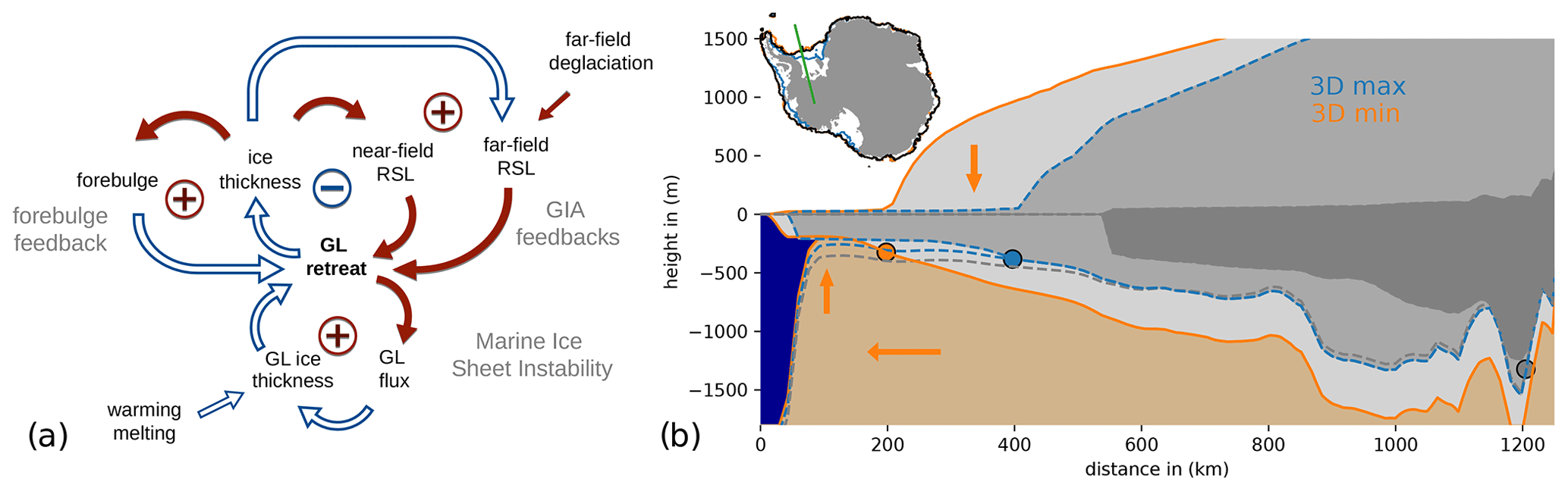
Figure 11 MISI and GIA feedbacks on grounding-line migration. (a) Feedback loops show the stabilizing near-field RSL feedback on grounding-line (GL) retreat (−) and the self-sustaining forebulge feedback (+) as well as the far-field (barystatic) RSL feedback (+). The marine ice sheet instability (MISI) represents a self-amplifying ice-internal feedback on GL retreat on retrograde slopes (+), which can be triggered by ocean-induced melting. Amplifying effects are indicated by filled red arrows (e.g., GL retreat leads to more GL flux), dampening effects are indicated by unfilled blue arrows (e.g., more GL flux results in less ice thickness at the GL). (b) Transect shows bedrock elevation and outlines of the ice sheet and ice shelf during the LGM through Ronne embayment from the continental shelf edge to the present-day GL position for the two Antarctic end-members of the reference 3D Earth structure, 3D max and 3D min. Respective GL positions (dots) are about 200 km apart. Orange arrows indicate additional ice mass, subsidence of the underlying bedrock, lateral displacement of mantle material and subsequent forebulge uplift (see also Video S2; Albrecht, 2024a). Dark-grey shading and dot indicate the present-day observed ice sheet configuration and GL position, respectively. Green line in inset indicates transect location.

When temperatures rise and the GL starts to retreat into overdeepened embayments, the marine ice sheet instability (MISI) supports a self-amplified GL retreat. With a thicker cross section, the GL flux increases non-linearly (Schoof, 2007), which reduces the ice thickness there and leads to further retreat (Fig. 11a). Our coupled simulations suggest that a weaker Earth structure causes a larger glacial-ice-sheet extent and more subsidence of the bedrock. This also implies an even steeper retrograde slope (Fig. 11b) and hence an increased potential for MISI-style GL retreat. However, gravitational changes and viscoelastic deformations due to GIA dampen the MISI feedback and slow down the retreat. This stabilizing “sea-level feedback” (e.g., Whitehouse et al., 2019) describes how loss in ice mass leads to lowering in RSL and hence to less GL retreat (see Fig. 11a). In our coupled simulations we did not consider the additional effects related to the marine ice cliff instability (MICI), whose relevance is under debate at the moment (Lipscomb et al., 2024).

Advancing and retreating GLs during Antarctic glacial cycles pass through roughly the same regions. The largest changes in grounded ice-sheet extent (and in RSL) are found in the Weddell Sea and Ross embayments, as well as in the Amundsen and Bellingshausen Sea in West Antarctica, while changes in East Antarctica are comparably small. The weakest Earth structure underneath Antarctica spans between Ross embayment and Amundsen Sea (see Fig. 5). The Earth material becomes stronger towards the Weddell Sea but is still weaker than the Antarctica-wide logarithmic mean. In the Ross Sea sector the present-day GL position seems loosely constrained by the geometry of the Siple Coast. This region also shows the weakest Earth structure in our setup, with a gradual and delayed modeled GL retreat until the present day (Neuhaus et al., 2021). We find here the lowest convergence rates in the iterative procedure (Fig. 4), defined as the relative reduction in RMSE between modeled present-day topography and observation in subsequent iterations, which is in line with the findings by van Calcar et al. (2023).

For GL advance during the glacial buildup, the Earth structure in all those West Antarctic regions seems to be weak enough to be supported by the forebulge feedback. The maximum LGM grounded ice-sheet extent from a coupled simulation with the Antarctica-wide minimum of the 3D Earth structure, 3D min, is similar to 3D ref. GL retreat during deglaciation tends to occur on much shorter timescales than during glacial buildup. However, due to the sea-level feedback, the retreat can be strongly slowed down in regions with a weak Earth structure, such as in the Ross Sea (Fig. 8). Yet, in the Weddell Sea and Bellingshausen Sea region, the MISI feedback seems to dominate the accelerated GL retreat. The resultant loss in SLRP seems to follow a trajectory which resembles a coupled simulation with the Antarctica-wide maximum or logarithmic mean of 3D ref, i.e., 3D max or “3D mean”, respectively (see Figs. 7 and S2). This implies that in most Antarctic regions 3D ref is not weak enough to obtain a significant delay of fast deglacial GL retreat due to the sea-level feedback and seems to be a robust feature, as we find a similar response of the AIS for an even larger variability in 3D Earth structures (Figs. S8–S10).

The strength of the solid Earth structure can be associated with a characteristic response timescale. In our coupled simulations we find a paradoxical behavior: a weak Earth structure with comparably short response times tends to support a slow glacial buildup, while it can slow down fast deglacial retreat. As we have a strongly heterogeneous 3D Earth structure, not only with large differences between East and West Antarctica but also with moderate differences within West Antarctica, we find a clear asymmetry in the aggregated response to 3D ref: the mantle material is weak enough to support the maximum LGM extent, while it is not weak enough to considerably slow down GL retreat. When performing iterations over two glacial cycles, this asymmetric response of the coupled system between glacial and deglacial phases requires larger adjustments in initial bed elevation for 3D ref than for 3D min, which then supports the glacial buildup in the next iteration and leads consequently to larger glacial ice volumes.

5 Conclusions

This study presents a new coupling framework between the ice sheet model PISM and the solid Earth model VILMA. We have run coupled simulations over two glacial cycles with PISM for Antarctica and VILMA with a global 3D viscosity structure. For coupling time steps of 100 years between PISM and VILMA, grid resolutions of 16 km for PISM in Antarctica, 0.2° (≤20 km) for solving the sea-level equation and 0.7° (≤78 km) for solving the viscoelastic deformations in VILMA, we are able to capture relevant dynamics and feedbacks in glacial-cycle simulations. We performed an iterative correction for initial topography over 246 kyr (two glacial cycles) to adjust for the initial bed topography. Much higher resolutions, as may be required for an adequate representation of the complex dynamics at the grounding line (GL) in some key regions, can be applied in this offline-coupling framework (e.g., 10-year coupling time step, on the order of 1 km for the ice dynamics and 0.1° resolution for the exchange of loading and the sea-level response); this is possible as the field equations in VILMA are solved in the time domain, which provides great flexibility with regard to restart states from which further simulations can be set up.

The tectonic setting of the Antarctic continent reflects strong lateral contrasts in the viscoelastic Earth structure. Our model study highlights the complexity of the interactions between ice sheets, sea level and the solid Earth in Antarctica and worldwide, given the spatial variability and uncertainty in the Earth structure and associated characteristic response timescales and length scales. We show that competing feedbacks and timescales are at play during Antarctic glacial buildup and deglaciation.

During phases of glacial buildup, when GLs advance over several tens of thousands of years, a forebulge can emerge in response to viscoelastic deformations. As the forebulge supports further GL advance, eventually up to the edge of the continental shelf, it defines a self-amplifying feedback on ice sheet growth – which we call the forebulge feedback.

In contrast, during deglaciation, GL retreat can be slowed down as a consequence of the sea-level feedback. In the case of a weak Earth structure, it implies that a fast and localized response of the solid Earth can slow down the retreat rate of the ice sheet. With a retrograde-sloping bed topography this stabilizing feedback can counteract the self-amplifying marine ice sheet instability, the latter favoring fast deglaciation. In the case of a stronger Earth structure and hence longer response timescales, we find rather slow and delayed uplift, which can even cause GL readvance, after it has stabilized at topographic features.

Understanding the interplay of feedback mechanisms and involved timescales is highly relevant for the stability analysis of the AIS in a warming climate. In particular, better constraints on the local Earth structure are required in key sensitive regions of West Antarctica. The GLs of the Amundsen Sea ice shelves (e.g., Pine Island and Thwaites) are likely entry points for the initialization of the West Antarctic Ice Sheet (WAIS) collapse, and also the stability of the Ross Sea and Weddell Sea is under discussion.

Our coupled model system yields self-consistent reconstructions of ice sheet and relative sea-level evolutions for 3D solid Earth structures. The modeled Antarctic sea-level rise potential during the Last Glacial Maximum relative to the present day shows a range between 10 and 15 m SLE for the different considered 3D Earth structures. These are slightly larger values than in recent coupled ice sheet–solid Earth reconstructions (Gomez et al., 2020; van Calcar et al., 2023) but within the range of previous model studies (Fig. 11b in Albrecht et al., 2020b). Based on the gained experience with PISM in high-resolution applications, this study adds confidence for the application of the PISM–VILMA coupling framework to future ice sheet evolution and sea-level projections and the investigation of tipping-point characteristics.